Evaluating methods to map burned area at 30-meter resolution in forests and agricultural areas of Central India

Biomass burning is a major phenomenon that plays an important role in small-scale ecological processes such as vegetation dynamics and soil erosion, and global processes such as hydrological cycles and climate change. However, global fire databases have low accuracies for burned area detection in areas with small fires, low biomass and in woodlands and open forests that characterize Central India. The present study uses higher resolution (30 meter) Landsat imagery to test accuracies for burned area detection using spectral indices (SI), machine learning (ML) algorithms and supervised classification. We find that detection of burned area by global fire product Fire Information for Resource Management System (FIRMS) is very low (<20%). Accuracies are higher for Landsat-based classification of burned area using supervised classification, random forest (RF) and Support Vector Machines (SVM). Accuracies are higher in April–May than in February–March and vary by azimuth angle on the day of image acquisition. RF produced the most consistently high classification accuracies for April (>80%), but had a tendency to misclassify less frequently available land covers; SVM had similar classification accuracies but had a tendency to overfit the model. Both lead to the potential for increasing commission errors and need to be used carefully when predicting burned area. Inclusion of SI had high relative importance in predicting burned area and reduced commission errors. Given these caveats, we recommend using ML algorithms for mapping burned area in the future, as it requires less time investment than classification and can yield consistent results. Accurate mapping of high-resolution fires is important for more accurate inputs into carbon inventories and ecological understanding of land-use dynamics and drivers.

1 Introduction

Biomass burning is a global environmental phenomenon with fires occurring in natural habitats such as tundras, savannas, deserts and forests, as well as human dominated landscapes such as agricultural fields. The size, timing, intensity and fuel in biomass burning influences land surface properties, atmospheric chemistry, vegetation cover (Bowman et al., 2009) and plays an important role in global processes such as hydrological cycles, soil erosion, radiation budget, and climate change (Chuvieco and Martin, 1994). Quantifying fires accurately is important to understand drivers of fire, and impact of fire on fragmentation, edge effects (Cochrane and Laurance, 2002) and biodiversity. Quantifying fires accurately is also crucial in studies on economics and health due to contribution of fires to pollution and health (Agarwala and Chandel, 2020; Singh P. et al., 2021). Finally, quantifying fires accurately is critical to create accurate carbon inventories to inform climate models (Shiraishi et al., 2021).

Remote sensing tools have been used to monitor and understand fire because many fire locations have low accessibility, and because of the dynamic nature and large extent of fires (Szpakowski and Jenson, 2019). Remote sensing tools have been used in varied ways to assist in fire risk mapping (Chuvieco and Congalton, 1989; Chuvieco and Martin, 1994), fuel mapping (Arroyo et al., 2008), active fire detection (Giglio et al., 2008), burned area estimates (Roy et al., 2008), burn severity assessment (Epting et al., 2005), and monitoring vegetation recovery (Fornacca et al., 2018) and its drivers (Gouveia et al., 2010). Climate inventories use global fire emissions databases such as Global Fire Emissions Database (GFED), Global Inventory for Chemistry-Climate Studies (GICC), and Global Fire Estimation System (GFAS) that are based on Moderate Resolution Imaging Spectroradiometer (MODIS) and Visible Infrared Imaging Radiometer Suite (VIIRS) Fire products (Singh D. et al., 2021). However, MODIS fire products report accuracies under 20% for fires, particularly because they are unable to identify small fires, although small fires are more widespread than large fires globally (Giglio et al., 2016). Such underestimation of fires compromises global carbon monitoring. Studies examining ecological processes are also compromised as fires may alter vegetation structure, plant species diversity and biomass carbon stocks (Hultquist et al., 2014). This suggests that there is a large scope for improvement of fire inventories for better climate modeling (Shiraishi et al., 2021).

The accuracies for fire prediction are particularly low in India. MODIS products have a low probability of fire detection in South East Asia and India, likely because fires are too small in these regions (Giglio et al., 2008, 2016). Other global products also either have fewer training data available in India (Fire_cci project)¹ or have low accuracies in similar ecosystems, such as in Africa (Ramo et al., 2018). Mapping and quantifying fires at high resolution is particularly important in India where 55% of forest areas are at risk of burning annually causing a total economic damage of $104 million (Chand et al., 2007; Forest Survey of India, 2019). A recent assessment for the state of Uttarakhand, in India, found that MODIS and VIIRS based products are only able to identify 5.64% of fire incidents due to their coarse scale (Kalaranjini et al., 2020). Within India, states in Central India (Andhra Pradesh, Chhattisgarh, and Madhya Pradesh) are most regularly affected by forest fires (Reddy et al., 2012), and have a high fire risk (Somashekar et al., 2009). Further, although frequency of forest fires is high in Central India, 55% of total biomass burning in the state of Madhya Pradesh was found to be in croplands, where small property sizes lead to small size of agricultural fires (e.g., Cusworth et al., 2018). Researchers also found an increasing trend in agricultural fires from 2002 to 2016 (Verma et al., 2019). Therefore, Central India has co-occurrence of small agricultural and forest fires in close proximity (Figure 1), which is important to quantify.

FIGURE 1

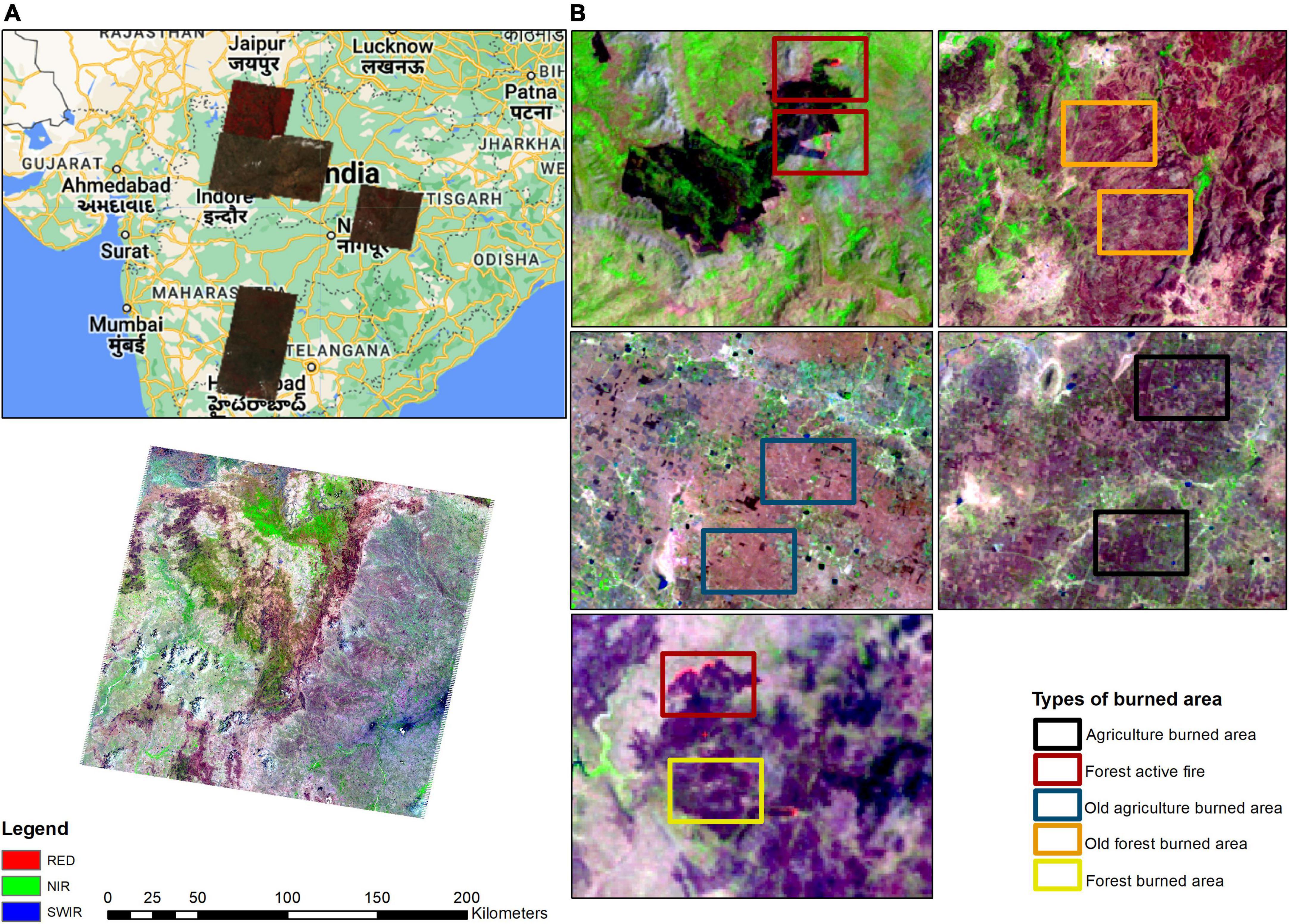
Figure 1. (A) Nine images selected for this study. (B) Landsat image (LT0514304520100329) showing variation in types of burned area in a landscape.

Use of high resolution (20-m) imagery increased detection of burned area by 80% compared with coarse resolution data in biomes similar to Central India in Africa. The difference in detection was more stark for smaller burn patches (<25 ha) where high resolution data detected 30 times more burned area (Roteta et al., 2019). Therefore, there is an urgent requirement for medium to high resolution fire mapping to better understand fire dynamics in India (Reddy et al., 2012). However, the vast majority of studies in India use MODIS based products or DMSP-OLS data for mapping fires at a coarse resolution (Chand et al., 2007; Singh et al., 2008). They are then used to either associate fires with air quality (Badarinath et al., 2007; Kharol et al., 2008), characterize agricultural burning patterns (Singh and Panigrahy, 2011; Verma et al., 2019), or predict forest fire risk (Somashekar et al., 2009; Giriraj et al., 2010; Renard et al., 2012; Jung et al., 2013). Studies that do attempt to quantify fire at a higher spatial resolution have mostly used Sentinel data (Babu et al., 2018; Kalaranjini et al., 2020; Singh D. et al., 2021), or data from Indian Remote Sensing Satellite (IRS-P6, AWiFS) (Reddy et al., 2012). As Sentinel data is only available since 2014, a long-term understanding of patterns in fire dynamics and its interaction with ecosystems requires burned area to be mapped at high resolution for periods before 2013 as well. While Landsat-based burned area products exist for some parts of the world (e.g., Loboda et al., 2018; Vetrita and Cochrane, 2019), there is no such product for India.

Because higher resolution imagery is less frequently available than MODIS products and VIIRS-derived Fire Information for Resource Management System (FIRMS) data, higher resolution imagery cannot rely on contrasting between thermal properties of fires and surrounding non-fire areas (Giglio et al., 2008, 2016; Schroeder et al., 2014). Instead, they rely on the different spectral properties associated with fire such as reduced chlorophyll, leaf tissue damage, decrease in crown shadow and moisture (Epting et al., 2005) and presence of charcoal residue (Fornacca et al., 2018). However, spectral properties may still allow burned area to be confused with other types of land surfaces such as water and shadow, and other land cover change processes such as selective logging and changing phenology (Epting et al., 2005). Classification accuracies differ by ecosystem (Epting et al., 2005) and region (Giglio et al., 2016). Central India is characterized by: small fires; a hilly terrain where shadows, contrasting topography, and heterogeneous landscapes that confounds analysis (Fornacca et al., 2018); forests with varying canopy cover (from very open forests with low tree cover to more dense woodlands); and a very high fire frequency. Hence, it is important to understand which methods would be most appropriate for identifying and quantifying fires (both agricultural and in the forest) in this region. Further, improved detection of burned area in such ecosystems is required as fires in grasslands, savannas and woodlands account for 60% of total carbon emissions (Shiraishi et al., 2021).

Methods used for mapping fires at high resolution in India are varied. Many scholars visually trace out fires or use local informants for mapping fires for smaller studies (Jung et al., 2013). Others use supervised classification based on maximum likelihood (Reddy et al., 2012; Ray et al., 2020), but supervised classification is not able to quantify fire severity. Supervised classification is also time-consuming and does not lend itself well to automation. Creating a burned area product for India cannot be done on individual images but will need to be automated and applied on multiple images to be available at large scales.

One method that lends itself well to large scale mapping of burned area across imagery is spectral indices (SI) as SI can be calculated easily from individual bands for any image. Use of SIs for burned area mapping focus on spectral bands that are most sensitive to fire and aim to reduce the noise in the signal (Fornacca et al., 2018). For example, decrease in chlorophyll following a fire may be associated with increase in reflectance in the visible spectrum, whereas leaf tissue damage may be associated with reduction in NIR reflectance (Pu and Gong, 2004). Decrease in crown shadow and canopy moisture may be associated with an increased reflectance in MIR (Epting et al., 2005). Spectral indices developed for burned area aim to capitalize on these differences and have high separability of burned and unburned area (Ba et al., 2019). While several indices have been known to perform well in areas with heterogeneous forest cover, low biomass and small fires (Fornacca et al., 2018), few studies exist for India. Studies on spectral indices for mapping burned area in India use only Normalized Difference Vegetation Index (NDVI), Normalized Burn Ratio (NBR), and Normalized Different Water Index (NDWI) as indices, that are used in combination to identify multiple thresholds for burned area mapping (Babu et al., 2018; Kalaranjini et al., 2020; Singh P. et al., 2021). Confusion between water and burned area still remains (Singh P. et al., 2021), which some scholars address by masking out water areas before quantifying fires (Babu et al., 2018). Alternatively, addition of these indices as inputs into a classification algorithm may increase classification accuracies (Pu and Gong, 2004; Ba et al., 2019).

A second method that has been used for mapping burned area and shows high accuracy is the use of machine learning (ML) algorithms such as Classification and Regression Tree (CART), random forest (RF) (Ramo et al., 2018; Roteta et al., 2019), support vector machine (SVM) (Petropoulos et al., 2011; Ramo et al., 2018), logistic regression (LR) (Pu and Gong, 2004), and Artificial Neural Networks (Ramo et al., 2018; Ba et al., 2019). ML algorithms can learn the spectral features of a sample of pixels with labels and recognize those patterns in other areas of the image (Ramo et al., 2018; Jain et al., 2020). ML algorithms have a further advantage in that they do not assume a normal data distribution (Belgiu and Drãguţ, 2016), and lend themselves well to automation. Scholars in India have begun using ML methods (Deshpande et al., 2022), but they have used MODIS data to help identify potential burned area. It is unclear how results will differ with use of more fine-scaled labels. Further, while ML-algorithms may be trained for classifying burned area in one image, given training data from sufficient numbers of images, it may be possible for ML algorithms to classify burned area in other images. This will require that we provide sufficiently representative images across space and time so that atmospheric and seasonal differences between images may also be included in the ML algorithms.

The present study focuses on using Landsat imagery to quantify burned area in forests and croplands in Central India. It has three objectives: first, we test whether accuracy of ML-based burned area mapping is as high as accuracy using supervised classification; and if so, we identify which parameters provide highest accuracy for each ML technique. Second, we test whether SIs have good separability for mapping burned area in Central India; and whether classification accuracies increase with addition of SIs to the training dataset. Finally, we use a larger number of images to test if accuracies differ by month of image acquisition, or other meta-data associated with image, to understand whether ML techniques can be applied across images of the same sensor to map burned area.

2 Materials and methods

2.1 Study area and imagery

Our study region was located in Central India, a region that has very high frequency of forest fires; many areas in Central India burn more than four times in ten years (Forest Survey of India, 2019). Dry deciduous forests in this area are highly susceptible to forest fires because of low soil moisture and a long dry pre-monsoon period which lasts for 5–6 months (Sannigrahi et al., 2020). Central India falls in sub-tropical climatic region with temperatures ranging from as low as 10°C in winters to as high as 48°C in summers. Mean annual rainfall at 1,160 mm is concentrated during the monsoon. This region has also seen an increase in agricultural burning (Verma et al., 2019).

Because the fires in the study region are small, one image contains both forest fires and agricultural fires (Figure 1), and these fires may have very different spectral properties (Figure 2). Further, highest frequency of forest fires is in March while highest frequency of agricultural fires is in April. This may result in any given image containing active fires, freshly burned area and older burned area (Figure 1). This variation may also confound identification of burned area due to variation in spectral properties between these types of burned area. This region also has strong seasonality as deciduous trees increasingly lose canopy from February to May (coinciding with burning period) with crops being harvested in April (also coinciding with burning period).

FIGURE 2

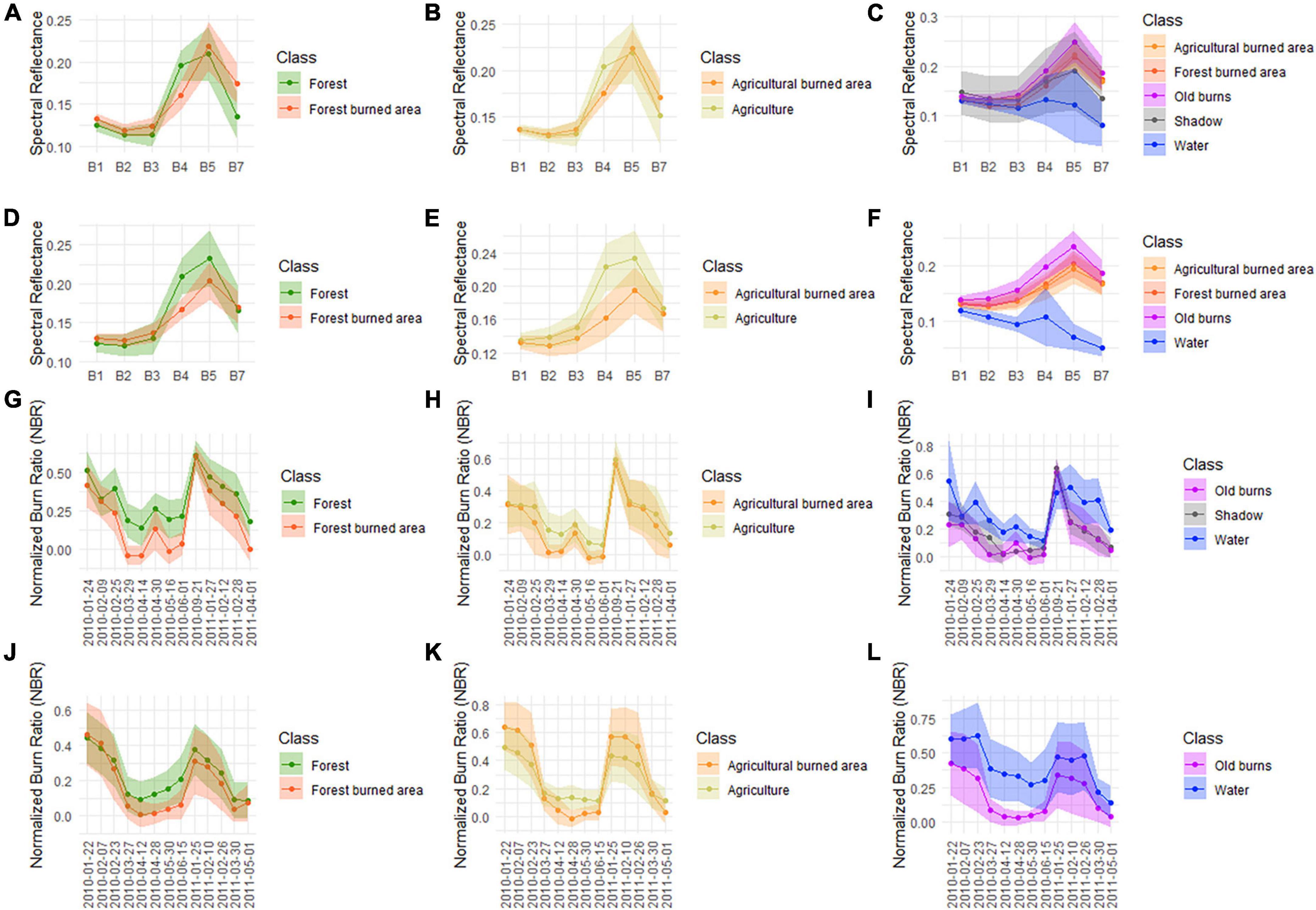
Figure 2. Spectral reflectance curves for Landsat image from March 2010 (LT0514304520100329) (A–C) and April 2010 (LT14504420100428) (D–F) show differences between forest areas and burned area in forests (A,D); differences in agricultural areas and burned agricultural areas (B,E); and between burned area in forests, burned area in agriculture, shadow, water and old burns (C,F). Trajectories for the March 2010 (G–I) and April 2010 (J–L) images show difference in normalized burn ratio (NBR) for one year between forests and burned area in forests (G,J); agriculture and burned area in agriculture (H,K); and old burns, shadow and water (I,L).

In order to select imagery that represents Central India spatially and temporally, we randomly selected 5 images to represent Central India (Figure 1). For this purpose, we downloaded the IDs of all Landsat 5 images in Central India from 1986 to present. We then divided the images into those in the fire season (those acquired from February to May). We then used R software (version 4.2.1) to randomly select 5 image IDs from the fire season. Final imagery selected ranged in time period from 1993 to 2011 (Supplementary Table 1).

In addition to these 5 images to represent the landscape, we chose two scenes from 2010 to represent crop burning and forest fires: Landsat 5 imagery from March 2010 represented peak forest burned area (LT0514345_20100329), and imagery from April 2010 (LT05145044_20100428) represented peak agricultural burned area. However, both images contain both types of burned area (Figure 1 and Supplementary Figure 1). These images were the first ones taken after peak fire (within 15 days). We then selected the most similar date for same path and row for 2009. Therefore, combining these images with the 5 randomly selected images, we used a total number of 9 Landsat scenes in our study (Supplementary Table 1).

For comparison with FIRMS data, we also downloaded the MODIS Collection 5 NRT Hotsport/Active Fire Detection MCD14DL product² for the same dates as the Landsat images. FIRMS data has a spatial resolution of 1,000 m, with daily temporal resolution, and is widely used in quantifying fires in India (Forest Survey of India, 2019).

2.2 Remote sensing

2.2.1 Image pre-processing

Landsat imagery (Collection 1, Level 1) was downloaded from NASA Earth Observation Data site. The Landsat images were calibrated to Top of the Atmosphere (Chavez, 1996) using ENVI 5.6 software. After calibration, all the bands other than thermal bands were stacked and masked before further analysis. For analysis in Google Earth Engine (GEE) platform, Collection 1 Level 1 TOA Reflectance data collection was used for analysis. Elevation data was collected from USGS (USGS/SRTMGL1_003) and was used to calculate slope and hillshade for each image for the day of image acquisition.

2.2.2 Calibration and validation datasets

For training and validation data, we used qGIS (version 3.16.13) to generate 700 random points at a minimum distance of 1 km from each other for each image. We then manually labeled 700 points as one of the following classes: burnt forest, unburnt forest, active fire in forest, forest area with leaf fallen off, burnt agriculture, unburnt agriculture, active fire in agriculture, agricultural area with no crops, water, shadow, cloud, old burns and others (built-up, barren land, and sandy areas). We included cloud and shadow to be able to later classify those areas where we had no data on fires as opposed to those areas where there was no fire. We included water as a separate label as it is often confused with burn scars. Identifying shadow was also important as it is also confused with burned area (Singh P. et al., 2021). We included forest area with leaf fallen off and agricultural area with no crops as labels because they are season-specific land classes that may otherwise confuse classification (Supplementary Figure 2). The discrimination between burnt and unburnt pixels was based on visual assessment of the image in SWIR, NIR, and Red bands, as has been done by many previous studies (e.g., Fornacca et al., 2018). However, as a secondary check on our labels, we also extracted values of spectral bands and spectral indices from January of that year to the following January to show the difference in spectral profiles of the different classes and the difference in their year-long trajectory (Figure 2). These trajectories show that points labeled as “old burns” are those that burnt a month prior to the date of image acquisition (Figure 2I). From these 700 points for each Landsat scene, 200 points were randomly selected using a random sample generator in R and saved as validation dataset (Dataset 1). Remaining 500 points were used as calibration dataset (Dataset 2) and are representative of actual distribution (e.g., Ramo et al., 2018) (see frequency distribution of class labels in Supplementary Table 2).

2.2.3 Spectral indices (SI)

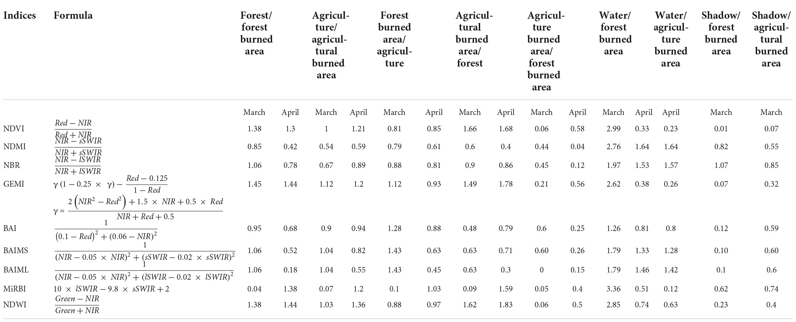
Inclusion of SIs in the training data significantly improves the accuracy of the burned area classification (Pu and Gong, 2004; Ba et al., 2019). We identified nine indices that are able to either identify burned area on their own or improve classification accuracies (Table 1). These include NDVI (Epting et al., 2005), NBR (Epting et al., 2005; Fornacca et al., 2018), Burned Area Index (BAI) (Martin et al., 2005; Fornacca et al., 2018; Parks and Abatzoglou, 2020), Normalized Difference Moisture Index (NDMI), Burn Area Index Modified-sSWIR (BAIMS), Burn Area Index Modified-lSWIR (BAIML) (Fornacca et al., 2018), Global Environmental Monitoring Index (GEMI) (Chuvieco et al., 2002; Fornacca et al., 2018), Mid-Infrared Burn Index (MiRBI) (Fornacca et al., 2018; Ba et al., 2019) and Normalized Difference Water Index (NDWI) (Reszka and Fuentes, 2015). Although difference Normalized Burn Ratio (dNBR) also has strong results (Babu et al., 2018; Fornacca et al., 2018), we excluded this index from our analyses due to its bi-temporality.

TABLE 1

Table 1. Ability of spectral indices to differentiate between LULC classes.

We used Dataset 1 to calculate M-statistics or signal-to-noise ratio (Table 1), which is defined as the difference between the means (μ) of two classes normalized by the total of their standard deviations (σ) (Fornacca et al., 2018; Ba et al., 2019; Roteta et al., 2019). M values greater than 1 indicate superior separation between the two classes, while values below 1 indicate inferior separation (Ba et al., 2019).

2.2.4 Supervised classification

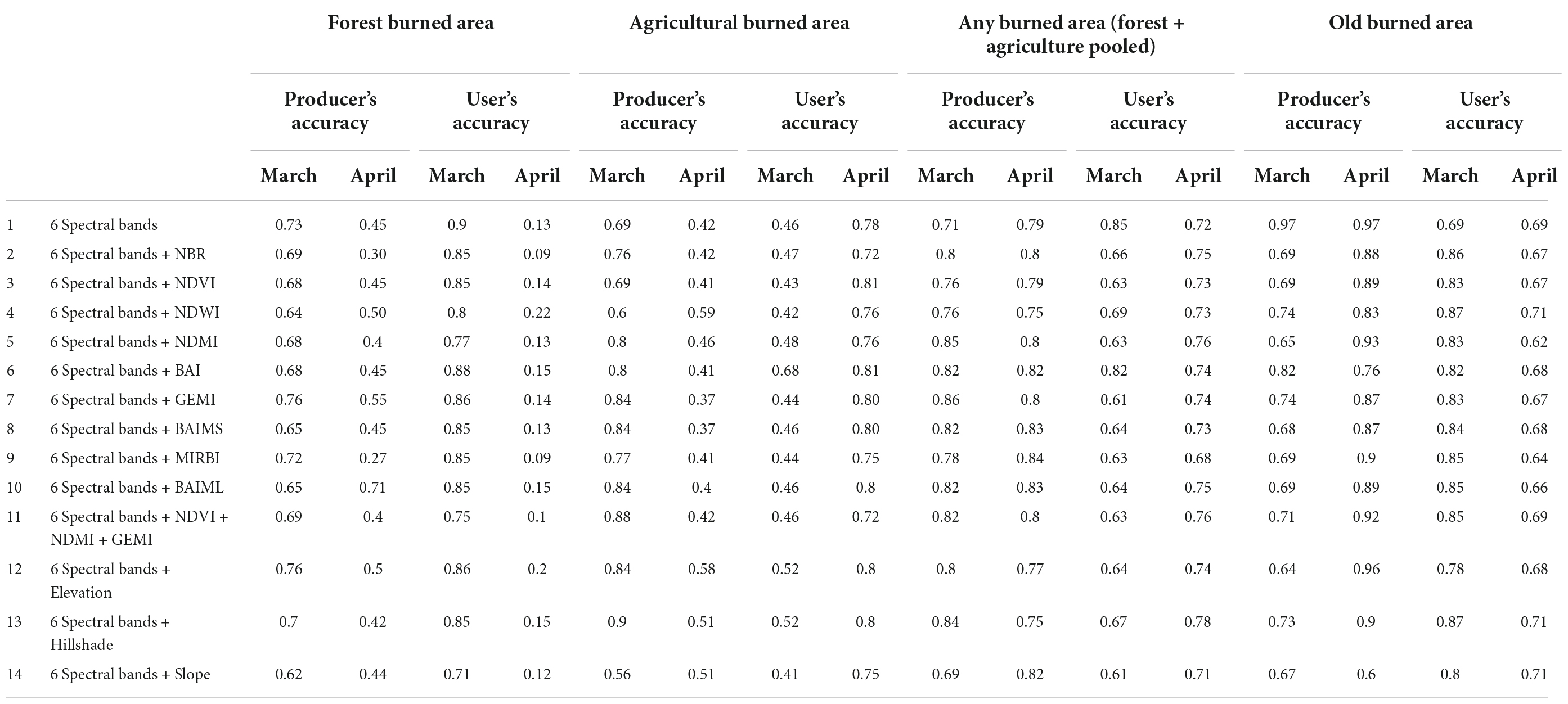
Since supervised classification using maximum likelihood is the most common method used to map burned area in India, we first tested the accuracies of burned area detection using supervised classification with maximum likelihood estimation. For this, we utilized Dataset 2 as training data to classify Landsat bands 1, 2, 3, 4, 5, and 7 into 13 classes, and used Dataset 1 to create a confusion matrix and evaluate accuracy. We then included SIs with high separability [from section “2.2.3 Spectral indices (SI)”] as inputs in our classification, to test if their inclusion improves accuracy (Table 2). Given the confusion between shadows and burned area, we also included hillshade as an input in our classification and tested whether inclusion of hillshade improves accuracy. Our classification used a threshold of 0.1 as it was providing the best results.

TABLE 2

Table 2. Accuracy assessment of supervised classification.

2.2.5 Machine learning algorithms

We tested the ability of two common ML techniques to classify burned area. The first was RF, one of the most extensively used LULC classifiers (Jain et al., 2020). RF is a supervised learning technique based on a decision tree; a decision tree is a series of if-then-else rules that can categorize pixels into burned or unburned. Decision trees are sensitive to training data and may overfit the model (Belgiu and Drãguţ, 2016). To reduce the overfitting of data and reduce bias, ensemble classifiers were developed that reduce susceptibility to noise by using bootstrapping or boosting (Belgiu and Drãguţ, 2016); RF is an ensemble classifier that uses bootstrapping. It produces multiple independent decision trees; each tree that classifies a pixel into a particular class acts as a vote for that pixel to belong to that class (Gislason et al., 2006; Hultquist et al., 2014; Jain et al., 2020). The advantages of RF are that it can successfully handle high data dimensionality and multicollinearity, is insensitive to overfitting (Belgiu and Drãguţ, 2016), and training algorithm is fast (Gislason et al., 2006). Within RF, we tested whether classification accuracy was influenced by number of trees (100 to 1000 at intervals of 100), number of variables per split (1 to 10 at intervals of 1), and bag fraction (0.1 to 1 at intervals of 0.1).

The second type of supervised learning ML technique we tested was SVM, which converts a non-linear problem to a linear one by using a kernel function to increase number of dimensions (Hultquist et al., 2014). It basically determines the best hyperplane for separating decision boundaries between different classes (Ramo et al., 2018), and is also one of the mostly commonly used ML algorithms for LULC classifications (Jain et al., 2020). We tested influence of kernel type [linear, polynomial, and radial basis function (RBF)] and penalization (0.1, 1, 10, and 100–1,000 at intervals of 100) on classification accuracy. For RBF, we further tested the role of gamma (0.05, 1). For polynomial, we also tested the role of degree (1,2,3,4). For hyperparameterization of both RF and SVM, we used Jupyter Notebook (jupyterlab 3.4.7; python version 8.5.0) and imported Google Earth Engine into python.

Although other ML algorithms exist and some, such as artificial neural networks, are used as often as RF and SVM for fire detection (Jain et al., 2020), the accuracies of SVM and RF are not biased by parameter selection as they are in artificial neural network (Ramo et al., 2018), and require less time in training than artificial neural networks. As a result, we limited our analysis to RF and SVM. Both ML algorithms included spectral bands, spectral indices and topography-derived variables such as slope and hillshade as input layers. We also quantified relative importance of different inputs in classification accuracy.

2.2.6 Potential for automating burned area detection across Central India

We expected that classification accuracy may vary due to differences in spectral reflectances because of conditions on the day of the image acquisition such as haze, solar position, season and location of image. Spectral reflectances may also vary because on-ground conditions may vary by month and location. To understand this, we classified each image using its own training data (Dataset 2), tested accuracy using its own validation data (Dataset 1), and checked how accuracy varies with factors related with position of sun such as solar elevation, azimuth angle and zenith angle, location-based factors such as path and row, and seasonal factors such as month. We then pooled the calibration data (Dataset 2) of all the 9 images to train a RF classifier to classify burned area in all the images. For this, we included scene-specific meta-data such as path ID, row ID, month of image acquisition, solar elevation and solar azimuth angle to the training data (we excluded solar zenith as it is calculated from solar elevation). We then applied this classifier to other images and tested accuracy using Dataset 1 of all the images.

3 Results

3.1 Separability of spectral indices

Separability of burned from unburned area varies with month of image acquisition and whether it is forest burned area or agricultural burned area (Table 1). For example, in March, GEMI and BAIML are able to separate forest burned area from both forest and agriculture (M-value > 1), NDVI and NDWI are able to separate forest burned area from forests, NBR is able to separate forest burned area from forest and shadow and BAI is able to separate forest burned area from agriculture (Table 1). However, by April, forest burned area can be differentiated from forests using NDVI, GEMI, NDWI, and only MiRBI can differentiate forest burned area from forest and agriculture. Fewer indices are also able to separate water from forest burned area.

For agricultural burned area, the impact of month of image is not as drastic. NDVI, GEMI, NDWI can all separate agricultural burned area from both forests and agriculture in both March and April. MiRBI can separate agricultural burned area from agriculture and forests only in April. No SI could separate forest burned area from agricultural burned area. Visually, the SIs appear to have very different outputs (Figure 3).

FIGURE 3

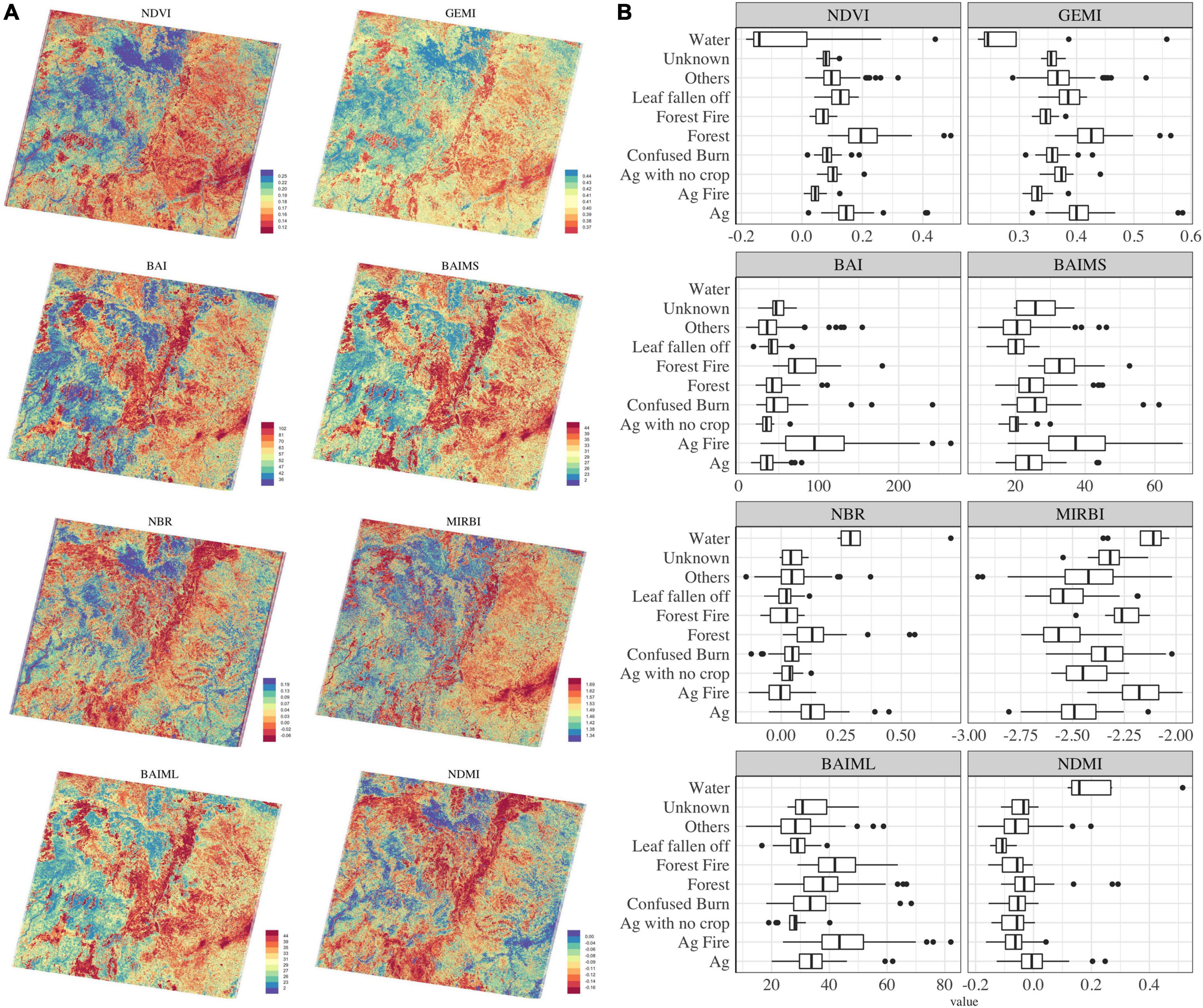
Figure 3. (A) Mapping burned area using different spectral indices, and (B) boxplots showing separability of different land use classes using different spectral indices. The images used in this figure are calculated from the March 2010 image; see Supplementary Figure 3 for similar figures for the April 2010 image.

3.2 Supervised classification

For supervised classification that used only spectral bands, results varied by month of image acquisition. In March, for forest burned area, producer’s accuracy is around 73% and the user’s accuracy is around 90%. Accuracies are much lower in April—producer’s accuracy is 45% and user’s accuracy is 13% (Table 2). For agricultural burned area, in March, the producer’s accuracy is 69% and user’s accuracy is 46%, but these are 42 and 78%, respectively in April. Overall, supervised classification is unable to differentiate between forest burned area and agricultural burned area. However, if we pool all burned area (burned area in both forest and agriculture), accuracy is much more consistent and ranges between 71 and 85% when using only spectral bands. Old burned area are confused with both forest burned area and agricultural burned area, but pooling old burned area with any other burned area (both agricultural and forest) only consistently increases producer’s accuracy and decreases user’s accuracy. Addition of elevation, hillshade and slope do not consistently increase accuracy (Table 2).

Supervised classification had sometimes very high and sometimes extremely low accuracies and is probably influenced by sampling bias in training data. In the March image, training data included sufficient points in water and shadow classes and the supervised classification was able to distinguish between water, shadow and burned area. In April image, the number of points in water did not exceed the number of bands in the training data, and hence dropped out of the classification. As a result, some water got classified as burned area in the supervised classification for April. In classifications where SIs were included, although classification accuracies are lower (varied between 63 and 82%), some water still got classified as burned area in April (Figure 4).

FIGURE 4

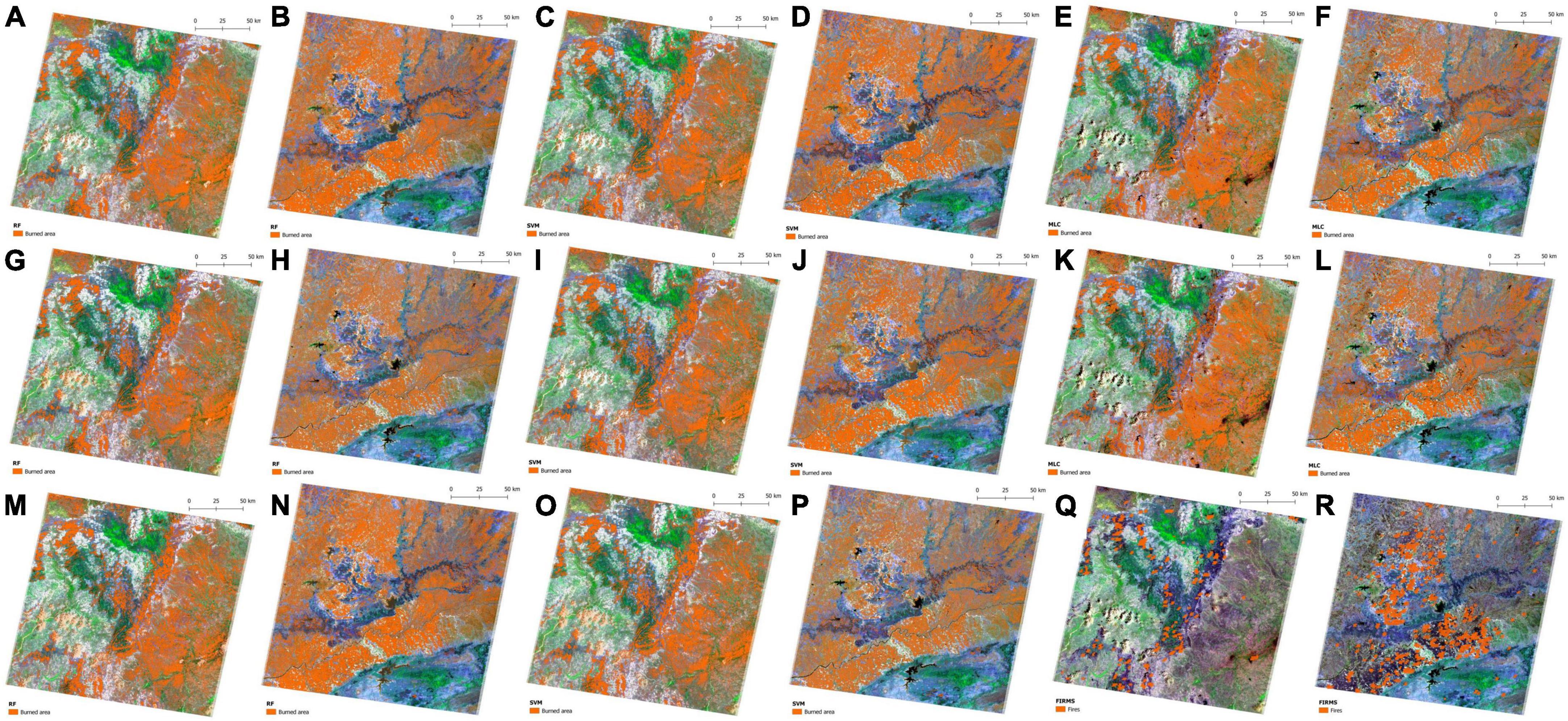
Figure 4. Classification results for models with highest producer’s accuracy (A–D), highest user’s accuracy (G–J) and models that maximize both producer’s and user’s accuracies (M–P) for RF (A,B,G,H,M,N) and support vector machine (SVM) (C,D,I,J,O,P). Results from supervised classification using only spectral bands (E,F), supervised classification that included NBR, NDVI and NDMI (K,L) and FIRMS (Q,R) included for comparison.

3.3 ML algorithms

3.3.1 Random forest

Results from RF were sensitive to parameter selection; some patterns are consistent across images while others are different for different images. Number of trees appears to have no association with accuracy. However, variation of bag fraction and number of variables per split with accuracies has different patterns for different images (Figures 5A–H).

FIGURE 5

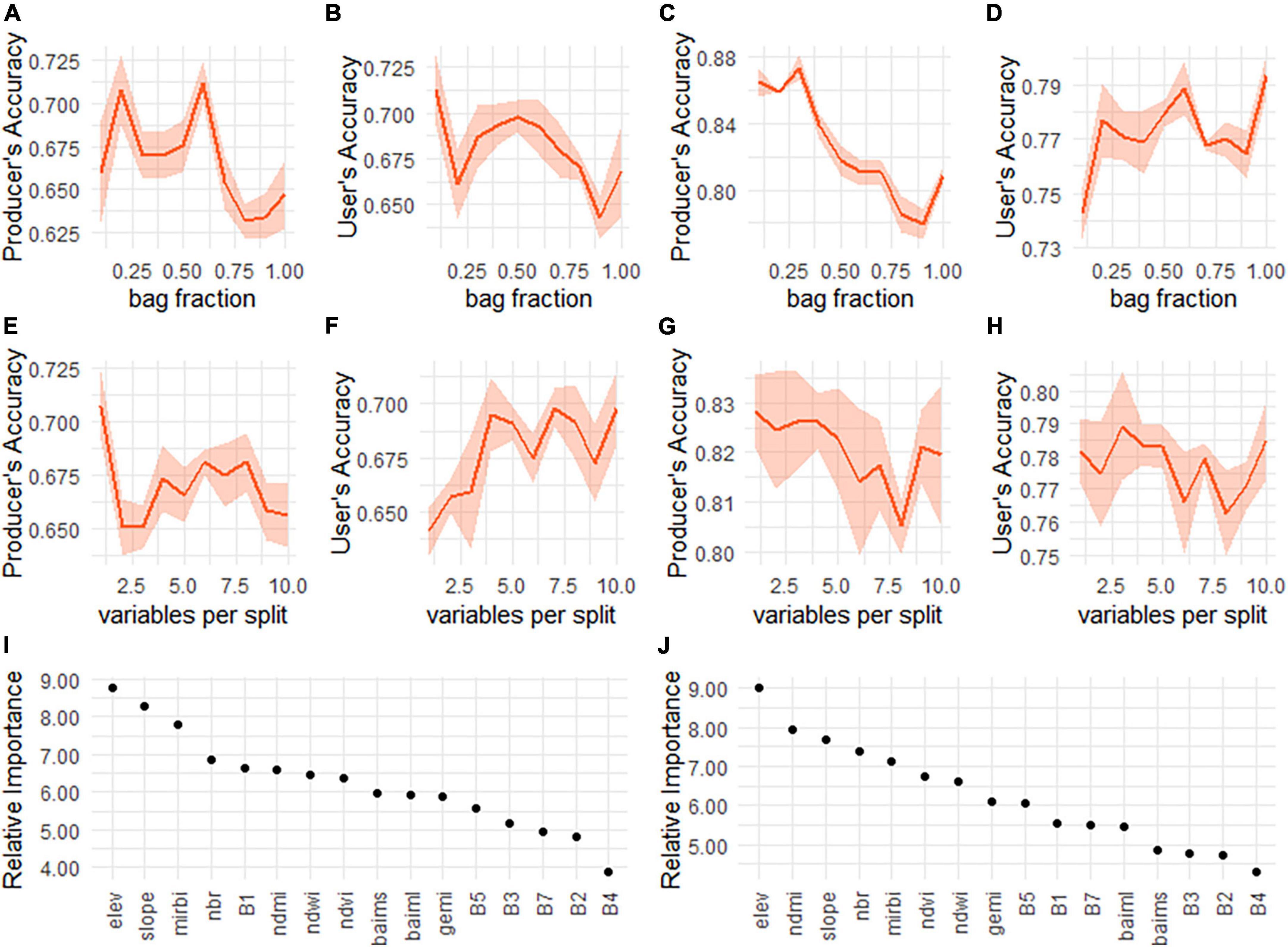
Figure 5. Influence of bag fraction on producer’s and user’s accuracy, where mean and confidence intervals are calculated for number of trees from 100 to 1,000 for number of variables per split equal to 7 (A–D). Influence of number of variables per split on producer’s and user’s accuracy, where bag fraction is 0.5 and mean and confidence intervals are calculated for number of trees from 100 to 1,000 (E–H) for March 2010 (A,B,E,F) and April 2010 (C,D,G,H) imagery. Relative importance of different variables for March 2010 image (I) and April 2010 image (J) for classifications with highest total accuracy.

This is reflected in the variation in results from RF (Figure 4). The highest producer’s accuracy for burned area (combining agriculture and forest burned area) for March is 0.75 and for April is 0.87, while the highest user’s accuracy for burned area in March is 0.77 and for April is 0.81. However, in choosing parameters that maximize either producer’s or user’s accuracy, RF misclassifies shadow as burned area in March image (Figure 4). When selecting parameters that maximize both producer’s and user’s accuracy, accuracy is lower at 0.73 and 0.82 producer’s accuracy for March and April, respectively, and 0.70 and 0.81 user’s accuracy for March and April. However, these parameters misclassify both water and shadows as burned area for March image but no water is classified as burned area for April image. All of these results are obtained using very different parameters (Table 3). In creating these results, SIs had higher relative importance than spectral bands, but the particular SIs that are more important are different for March and April (Figures 5I,J).

TABLE 3

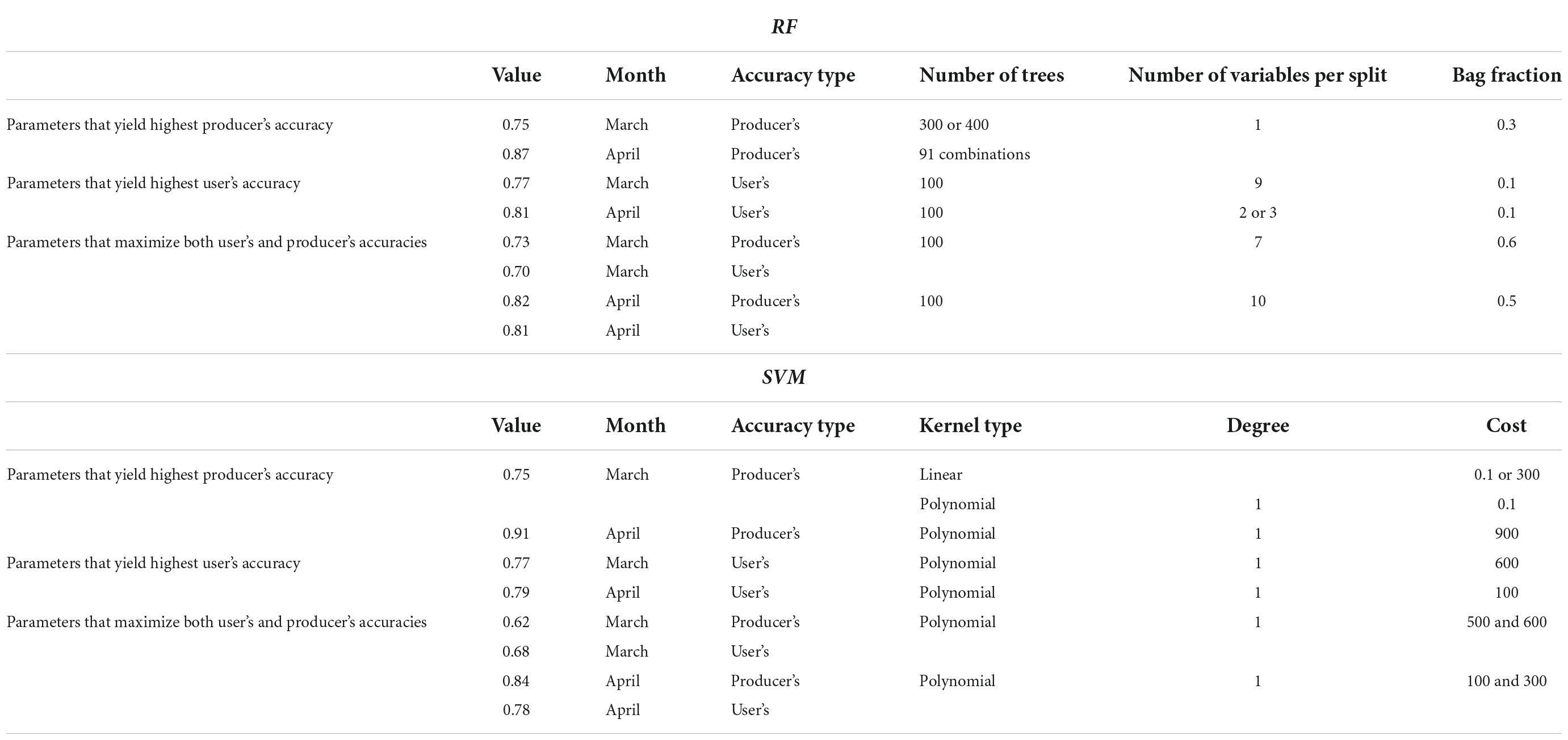
Table 3. Variation in ML parameters that yield highest producer’s accuracy, highest user’s accuracy, and maximize both producer’s and user’s accuracies.

One advantage of RF appears to be that it is not limited by the minimum number of samples per class. In April image, where water had dropped out of the supervised classification due to insufficient training data points, water does get included in RF classification and is able to distinguish between water and burned area when we select parameters that yield highest user’s accuracy and when we select parameters that maximize both user’s and producer’s accuracies.

3.3.2 Support vector machine

The highest producer’s accuracy for burned area for March is 0.77 and for April is 0.91, while the highest user’s accuracy for burned area in March is 0.77 and for April is 0.79. If we tabulate hyperparameterization results for SVM, some accuracy values may be outliers at upto 9% points above others (Supplementary Figure 4). As SVM does not use any bagging techniques, it may be overfitting the data and obtaining anomalously high accuracies which overestimate burned area (e.g., user’s accuracy in April, Figure 4J). If we select the model parameters that have the highest user’s and producer’s accuracies but are not outliers, then we obtain accuracies of 0.62 and 0.68 for March and 0.84 and 0.78 for April. These still classify water and shadows as burned area in March, but do not classify water as burned area in April.

Results from SVM were not as sensitive to parameter selection as RF: for linear kernel type, increasing cost was associated with an oscillating pattern for both producer’s accuracy and user’s accuracy (Figure 6); for RBF kernel type, cost did not have much impact on accuracy above a cost of 100 (Supplementary Figure 5.1). For polynomial kernel type, increasing degree was associated with lower accuracy for both March and April image (Figure 6).

FIGURE 6

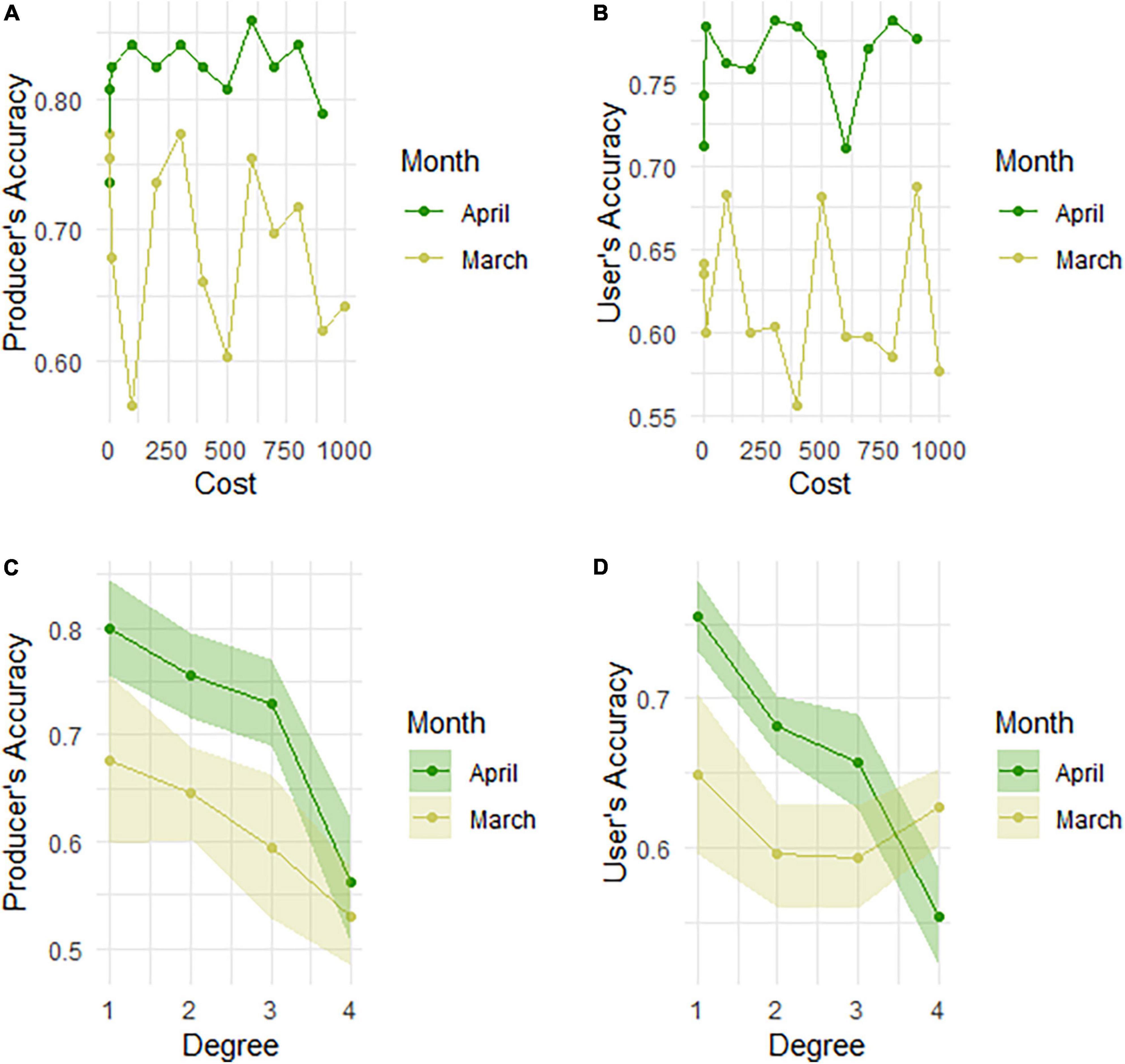
Figure 6. Variation in accuracy for linear kernel type (A,B) and polynomial kernel type (C,D) in SVM.

Support vector machine results are obtained using slightly similar parameters (Table 3). Linear kernel type and polynomial kernel type often result in similarly high accuracies, but misclassification of water and shadows as burned area is higher in linear kernel type (Supplementary Figure 5.2). Qualitatively, SVM performed better at differentiating between water, shadow and burned area than RF in April image, but it has a tendency to overfit the data. Water did not get classified as burned area in April image for parameters that maximize both highest producer’s and user’s accuracies.

3.4 Comparison with FIRMS

In comparison to Landsat-based methods, commonly used FIRMS data has very low accuracy. Detection of forest fire was better than detection of agricultural fires in the month where forest fires were more frequent, and detection of agricultural fires was better in the month where agricultural fires were more frequent (Table 4 and Figure 4). Further, FIRMS did not get water and shadow confused with burned area.

TABLE 4

Table 4. Comparison of user’s accuracies across different methods.

3.5 Potential for automating burned area detection across Central India

Classification accuracy appears to decrease with azimuth angle of image and increase with month (Figure 7). Within this, classification accuracy of forest fire does not vary systematically with month and azimuth angle, while classification of agricultural burned area is low at higher azimuth angle and earlier in the year when agricultural burning has lower incidence (Supplementary Figure 6). When we use training data from all the images together for classification, the most important scene-specific variables in the classification were solar azimuth at 4^th position, solar elevation at 12th position and month at 18th position (Figure 7). They contributed 21.89, 18.86, 12.13%, respectively to the classification accuracy. Relative importance varies with different runs of the model, but these variables are consistently important. This suggests that accounting for this meta-data may allow higher accuracy for classification of multiple images.

FIGURE 7

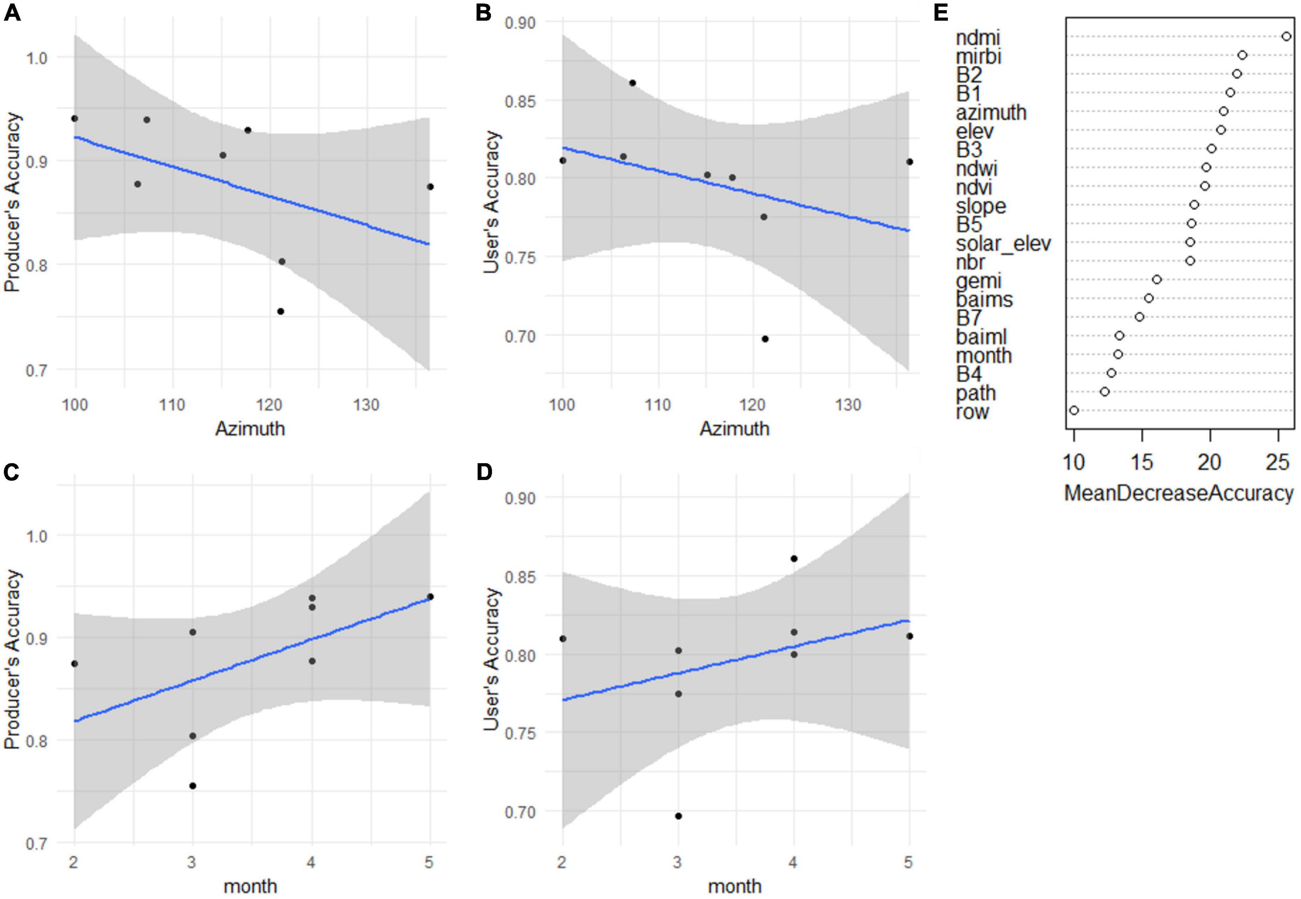
Figure 7. Change in (A) producer’s accuracy with azimuth angle, (B) user’s accuracy with azimuth angle, (C) producer’s accuracy with month of image acquisition, (D) user’s accuracy with month of image acquisition, and (E) relative contribution of image-associated meta-data to accuracy of burned area classification across all images.

4 Discussion

4.1 Spectral indices

SIs did not perform consistently when used in isolation. While the literature focuses on NBR and BAI, NBR and BAI did not perform very well. NBR performs better when biomass is higher; in literature, classification of burned area had 10% higher accuracy in forests than in non-forest areas (Epting et al., 2005). This may explain poor separation of burned area in April when leaf fall in deciduous trees implies lower forest biomass, thus lower separability for NBR. Absence of a pre-burn reference may also have led to confusing features such as water, senescent vegetation and older fire scars—which have similar spectral properties—with new fire scars (Epting et al., 2005). One advantage of NBR, though, is its ability to separate forest burned area and shadows in March. Poor performance of BAI may be due to it being developed for coarser resolution AVHRR imagery, but it has previously performed well with Landsat imagery (Fornacca et al., 2018). Further, BAI prioritizes the spectral signature of charcoal (Fornacca et al., 2018), which may be absent in agricultural fields if the field is plowed soon after burning. Charcoal may also be low in forest burned area if forest fires do not leave sufficient charcoal residue visible from above the canopy, as may be the case in this region due to small fires that are often limited to the understory. Instead, high separability between burned and unburned area (M-value>1) was more consistently achieved by indices such as GEMI, NDVI, and NDWI. These indices performed well because vegetation is higher in unburned area; tellingly, NDVI performed worse in both agricultural and forest burned area in April when vegetation was lower. Because GEMI and NDVI appear to be capturing the loss of vegetation aspect of burned area, they cannot be used in isolation.

Although inclusion of SIs did not consistently increase classification accuracy of burned area using supervised classification, SIs had higher relative importance when using ML algorithms for classification. Three types of SIs appear to be playing a role in classification: those that differentiate burned area from unburned area because vegetation is higher in unburned area (such as GEMI, NDVI); those that differentiate burned area from unburned area due to other factors such as shadows (such as NBR, MiRBI); and those that differentiate burned area from water (such as NDMI, NDWI). The importance of SIs is reflected in results from ML algorithms where NDMI, MiRBI, NDVI and NBR consistently show up as important, followed by NDWI and GEMI. The incorporation of these indices probably helps account for other important variables associated with fires such as change in vegetation, charcoal and moisture (Ba et al., 2019), and reduces or eliminates other confounding factors such as soil and atmospheric effects (Pu and Gong, 2004).

4.2 Classifying agricultural and forest burned area

Machine learning algorithms had more consistent results than supervised classification. This may be because of several reasons. First, supervised classification, particularly those using maximum likelihood estimations, assumes normal data distribution which may not always be the case and lead to erroneous analysis (Belgiu and Drãguţ, 2016). ML algorithms also require less training data than supervised classification, which requires a minimum number of training data per class in order to use it in classification. This meant that supervised classification was unable to classify water and shadow when training data was unbalanced. It also meant that low frequency of forest fires in April led to lower classification accuracy in quantifying forest burned area (13%), whereas ML algorithms could identify the same with an accuracy of over 75% (Table 4).

Of the two ML algorithms tested, RF had more consistent results than SVM if we choose the parameters with the highest accuracy for both producer’s and user’s accuracies. SVM can result in outlier accuracy values for certain parameters that are ∼9% points above the next accuracy value (Supplementary Figure 4). For SVM, results are consistent if we choose parameters with highest producer’s and user’s accuracies after excluding outliers. This difference between RF and SVM is probably because RF accounts for decision tree’s known limitation of being influenced by noise and overfitting the model (Belgiu and Drãguţ, 2016), by virtue of being an ensemble classifier. Previous research has also found that RF was marginally better than SVM (Hultquist et al., 2014), although RF’s known disadvantage is that it is sensitive to sampling design (Belgiu and Drãguţ, 2016). This is also reflected in the fact that RF misclassified classes that are less frequently present in the landscape, such as water and shadow, in certain parameters, which SVM did not. Overall, for best RF results, we should use parameters that maximize both user’s and producer’s accuracies. Other parameters may lead to misclassification of less frequently present land-cover types. For best SVM results, we must exclude parameters that result in outlier accuracy values, otherwise SVM algorithm may overestimate the more frequently present land covers like burned area (as in Figure 4J).

Although the two ML algorithms used different approaches to learning (Jain et al., 2020), both ML algorithms gave accuracy results comparable with or better than supervised classification. This may be because the ML algorithm was able to use differentiation on multiple parameters, including information from indices included as layers in the analysis. Although the ability of ML algorithms to capture non-linear patterns (Jain et al., 2020) did lead to more consistent results than the supervised classification, the reduced time invested in the method and its capacity for automation make it a more attractive option when considering a method for identifying and quantifying burned area over larger landscapes encompassing more than one image.

Overall, accuracy for burned area detection using Landsat imagery was ∼70% for March and ∼80% for April using ML techniques (detailed in section “4.3 Seasonal effects”). These are lower than previous studies that report accuracies >90%. Our results may be lower because we used an external validation dataset instead of using bagging to calculate accuracy. Additionally, forests in the study region had a hilly terrain with hill shadows, water bodies and dense broadleaved trees that may have increased the noise and induced errors in detection (Fornacca et al., 2018). Further, forests of Central India closely resemble woodlands or savanna due to their openness (Ratnam et al., 2011); woodlands have a more variable response to fires and may range from resprouting shrubs to becoming unvegetated (this is very different from forested pixels that give a consistent spectral signal of charred boles and branches) (Epting et al., 2005). Also, agricultural areas in the study region had small settlements with possibly small fires that may induce errors in identifying cropland fires.

4.3 Seasonal effects

Classification accuracies for images acquired in March and April had consistently different results (∼70% for March and ∼80% for April using ML techniques). This may be due to several reasons. One set of reasons is because of actual differences in fire on the ground. For example, peak agricultural burning is in April when forest fire is less frequent and peak forest fires are in March when agricultural burning is less frequent. This alters sampling frequency as training data in April may have less samples of forest burned area, as forest burned area is less frequent in that month. The forest biomass itself is lower in April due to the deciduous nature of the forest. Many of these techniques work better when biomass is higher; for example, NBR performs better when biomass is higher (Epting et al., 2005).

The second set of reasons appears to be associated with the day conditions where accuracy appears to increase later in the season (Figure 7). However, on closer examination, agricultural fires have a lower accuracy before April whereas there is not much variation in classification accuracy of forest burned area across the seasons (Supplementary Figure 6). This suggests that we should choose images later in the season, in April or May, when automating burned area detection across the region.

4.4 Comparison with FIRMS data

Fire Information for Resource Management System had accuracies under 20% in all conditions. Similar accuracies were obtained for Landsat only in supervised classification when the frequency of forest fires was very low. In comparison, ML algorithms that used Landsat consistently had accuracies over 70% for single image classifications. FIRMS underestimates burned area by at least one fourth with implications for poor understanding of large-scale drivers and patterns of forest fires. Given high rate of increase of crop residue burning in India (Verma et al., 2019), underestimation of agricultural burning also has significant implications for misunderstanding patterns and drivers and misinforming policy. This study shows that use of Landsat imagery may help identify burned area at higher accuracy across the region. In doing so, overall accuracy is likely to be higher if we focus on images later in the fire season (April-May). Incorporation of image-associated meta-data is likely to allow classification of images for which training data is not present, thus allowing large-scale mapping of burned area.

Overall, since accuracies using Landsat-based imagery is so much higher for burned area than FIRMS, in choosing a method, we must prioritize commission errors over omission errors. Increasing accuracy from <20 to >70% is a significant increase in fire detection, but it will be compromised if our commission error rate is high. Of the two ML techniques, RF is highly sensitive to parameter selection, and can tend to misclassify less frequently present land-covers. Since previous research has been troubled by misclassification of water and shadow as burned area, the commission errors due to this in RF have a potential to be high. On the other hand, while SVM does not appear to have this problem, it has a tendency to overfit the model and misclassify non-burned area as burned area earlier in the season. We must be careful when applying either SVM or RF to opt for lower accuracy and prioritize limiting commission errors for the burned area product to be an improvement on FIRMS.

Data availability statement

The raw data supporting the conclusions of this article will be made available by the authors, without undue reservation.

Author contributions

AC, SD, and MA conceptualized the project. AC, WS, AN, and MA did the data collection and analysis. AC, WS, and MA wrote the manuscript. All authors contributed to the article and approved the submitted version.

Acknowledgments

The staff on this project were supported by City Knowledge Innovation Cluster, Delhi Research Implementation and Innovation (DRIIV), an initiative of the Office of the Principal Scientific Adviser to the GoI, and Centre for Climate Change and Sustainability, Ashoka University.

Conflict of interest

The authors declare that the research was conducted in the absence of any commercial or financial relationships that could be construed as a potential conflict of interest.

Publisher’s note

All claims expressed in this article are solely those of the authors and do not necessarily represent those of their affiliated organizations, or those of the publisher, the editors and the reviewers. Any product that may be evaluated in this article, or claim that may be made by its manufacturer, is not guaranteed or endorsed by the publisher.

Supplementary material

The Supplementary Material for this article can be found online at: https://www.frontiersin.org/articles/10.3389/ffgc.2022.933807/full#supplementary-material

Footnotes

1. ^ http://www.esa-fire-cci.org
2. ^ https://earthdata.nasa.gov/firms; doi: 10.5067/FIRMS/MODIS/MCD14DL.NRT.00

References

Agarwala, M., and Chandel, A. (2020). Temporal role of crop residue burning (CRB) in Delhi’s air pollution. Environ. Res. Lett. 15:13. doi: 10.1088/1748-9326/abb854

CrossRef Full Text | Google Scholar

Arroyo, L. A., Pascual, C., and Manzanera, J. A. (2008). Fire models and methods to map fuel types: The role of remote sensing. For. Ecol. Manage. 256, 1239–1252.

Google Scholar

Ba, R., Song, W., Li, X., Xie, Z., and Lo, S. (2019). Integration of multiple spectral indices and a neural network for burned area mapping based on MODIS data. Remote Sens. 11:326. doi: 10.3390/rs11030326

CrossRef Full Text | Google Scholar

Babu, S. K. V., Roy, A., and Aggarwal, R. (2018). Mapping of forest fire burned severity using the sentinel datasets. Int. Arch. Photogramm. Remote Sens. Spat. Inf. Sci. XLII-5, 469–474. doi: 10.5194/isprs-archives-XLII-5-469-2018

CrossRef Full Text | Google Scholar

Badarinath, K. V., Kharol, S. K., and Chand, T. R. (2007). Use of satellite data to study the impact of forest fires over the Northeast Region of India. IEEE Geosci. Remote Sens. Lett. 4, 485–489. doi: 10.1109/lgrs.2007.896738

CrossRef Full Text | Google Scholar

Belgiu, M., and Drãguţ, L. (2016). Random forest in remote sensing: A review of applications and future directions. ISPRS J. Photogramm. Remote Sens. 114, 24–31. doi: 10.1016/j.isprsjprs.2016.01.011

CrossRef Full Text | Google Scholar

Bowman, D. M. J. S., Balch, J. K., Artaxo, P., Bond, W. J., Carlson, J. M., Cochrane, M. A., et al. (2009). Fire in the earth system. Science 324, 481–485.

Google Scholar

Chand, T. R., Badarinath, K. V. S., Murthy, M. S. R., Rajshekhar, G., Elvidge, C. D., and Tuttle, B. T. (2007). Active forest fire monitoring in Uttaranchal State, India using multi-temporal DMSP-OLS and Modis data. Int. J. Remote Sens. 28, 2123–2132. doi: 10.1080/01431160600810609

CrossRef Full Text | Google Scholar

Chavez, P. S. (1996). Image-based atmospheric corrections–revisited and improved. Photogramm. Eng. Remote Sens. 62, 1025–1036.

Google Scholar

Chuvieco, E., and Congalton, R. G. (1989). Application of remote sensing and geographic information systems to forest fire hazard mapping. Remote Sens. Environ. 29, 147–159. doi: 10.1016/0034-4257(89)90023-0

CrossRef Full Text | Google Scholar

Chuvieco, E., and Martin, M. P. (1994). Global fire mapping and fire danger estimation using AVHRR images. Photogramm. Eng. Remote Sens. 60, 563–570.

Google Scholar

Chuvieco, E., Martin, M. P., and Palacios, A. (2002). Assessment of different spectral indices in the red–near-infrared spectral domain for burned land discrimination. Int. J. Remote Sens. 23, 5103–5110. doi: 10.1080/01431160210153129

CrossRef Full Text | Google Scholar

Cochrane, M. A., and Laurance, W. F. (2002). Fire as a large-scale edge effect in Amazonian forests. J. Trop. Ecol. 18, 311–325. doi: 10.1017/S0266467402002237

CrossRef Full Text | Google Scholar

Cusworth, D. H., Mickley, L. J., Sulprizio, M. P., Liu, T., Marlier, M. E., DeFries, R., et al. (2018). Quantifying the influence of agricultural fires in northwest India on urban air pollution in Delhi, India. Environ. Res. Lett. 13:044018.

Google Scholar

Deshpande, M. V., Pillai, D., and Jain, M. (2022). Agricultural burned area detection using an integrated approach utilizing multi spectral instrument based fire and vegetation indices from sentinel-2 satellite. MethodsX 9:101741. doi: 10.1016/j.mex.2022.101741

PubMed Abstract | CrossRef Full Text | Google Scholar

Epting, J., Verbyla, D., and Sorbel, B. (2005). Evaluation of remotely sensed indices for assessing burn severity in interior Alaska using Landsat TM and ETM+. Remote Sens. Environ. 96, 328–339. doi: 10.1016/j.rse.2005.03.002

CrossRef Full Text | Google Scholar

Forest Survey of India (2019). Forest fire monitoring, in India state of forest report 2019. Dehradun: Forest Survey of India, 87–99.

Google Scholar

Fornacca, D., Ren, G., and Xiao, W. (2018). Evaluating the best spectral indices for the detection of burn scars at several post-fire dates in a Mountainous Region of Northwest Yunnan, China. Remote Sens. 10:1196. doi: 10.3390/rs10081196

CrossRef Full Text | Google Scholar

Giglio, L., Csiszar, I., Restás, Á, Morisette, J. T., Schroeder, W., Morton, D., et al. (2008). Active fire detection and characterization with the advanced spaceborne thermal emission and reflection radiometer (ASTER). Remote Sens. Environ. 112, 3055–3063. doi: 10.1016/j.rse.2008.03.003

CrossRef Full Text | Google Scholar

Giglio, L., Schroeder, W., and Justice, C. O. (2016). The collection 6 MODIS active fire detection algorithm and fire products. Remote Sens. Environ. 178, 31–41. doi: 10.1016/j.rse.2016.02.054

PubMed Abstract | CrossRef Full Text | Google Scholar

Giriraj, A., Babar, S., Jentsch, A., Sudhakar, S., and Sri Ramachandra Murthy, M. (2010). Tracking fires in India using advanced along track scanning radiometer (A)ATSR data. Remote Sens. 2, 591–610. doi: 10.3390/rs2020591

CrossRef Full Text | Google Scholar

Gislason, P. O., Benediktsson, J. A., and Sveinsson, J. R. (2006). Random forests for land cover classification. Pattern Recognit. Lett. 27, 294–300. doi: 10.1016/j.patrec.2005.08.011

CrossRef Full Text | Google Scholar

Gouveia, C., DaCamara, C. C., and Trigo, R. M. (2010). Post-fire vegetation recovery in Portugal based on spot/vegetation data. Nat. Hazards Earth Syst. Sci. 10, 673–684. doi: 10.5194/nhess-10-673-2010

CrossRef Full Text | Google Scholar

Hultquist, C., Chen, G., and Zhao, K. (2014). A comparison of Gaussian process regression, random forests and support vector regression for burn severity assessment in diseased forests. Remote Sens. Lett. 5, 723–732. doi: 10.1080/2150704X.2014.963733

CrossRef Full Text | Google Scholar

Jain, P., Coogan, S. C. P., Subramanian, S. G., Crowley, M., Taylor, S., and Flannigan, M. D. (2020). A review of machine learning applications in wildfire science and management. Environ. Rev. 28, 478–505. doi: 10.1139/er-2020-0019

CrossRef Full Text | Google Scholar

Jung, J., Kim, C., Jayakumar, S., Kim, S., Han, S., Kim, D., et al. (2013). Forest fire risk mapping of Kolli Hills, India, considering subjectivity and inconsistency issues. Nat. Hazards 65, 2129–2146. doi: 10.1007/s11069-012-0465-1

CrossRef Full Text | Google Scholar

Kalaranjini, V. S., Dinesh Kumar, S., Ramakrishnan, S., and Kokila Priya, R. (2020). “Burnt area detection using SAR data–a case study of May, 2020 Uttarakand Forest fire,” in Proceedings of the 2020 IEEE India geoscience and remote sensing symposium (InGARSS), (Ahmedabad: IEEE). doi: 10.1109/ingarss48198.2020.9358979

CrossRef Full Text | Google Scholar

Kharol, S. K., Badarinath, K. V. S., and Roy, P. S. (2008). “Studies on emissions from forest fires using multi-satellite datasets over north east region of India,” in Proceedings of the International Archives of the Photogrammetry, Remote Sensing and Spatial Information Sciences, XXXVII. Part B8. Beijing, 473–478.

Google Scholar

Loboda, T. V., Chen, D., Hall, J. V., and He, J. (2018). ABoVE: Landsat-derived burn scar dNBR across Alaska and Canada, 1985-2015. Oak Ridge, TN: ORNL DAAC. doi: 10.3334/ORNLDAAC/1564

CrossRef Full Text | Google Scholar

Martin, P., Gomez, L., and Chuvieco, E. (2005). “Performance of a burned-area index (BAIM) for mapping Mediterranean burned scars from MODIS data,” in Proceedings of the 5th International workshop on remote sensing and GIS applications to forest fire management: Fire effects assessment: 193-197, eds J. De la Riva, F. Pérez-Cabello, and E. Chuvieco (Zaragoza: Universidad de Zaragoza).

Google Scholar

Parks, S. A., and Abatzoglou, J. T. (2020). Warmer and Drier fire seasons contribute to increases in area burned at high severity in Western US forests from 1985 to 2017. Geophys. Res. Lett. 47:e2020GL089858. doi: 10.1029/2020GL089858

CrossRef Full Text | Google Scholar

Petropoulos, G. P., Kontoes, C., and Keramitsoglou, I. (2011). Burnt area delineation from a uni-temporal perspective based on landsat TM imagery classification using support vector machines. Int. J. Appl. Earth Obs. Geoinf. 13, 70–80. doi: 10.1016/j.jag.2010.06.008

CrossRef Full Text | Google Scholar

Pu, R., and Gong, P. (2004). Determination of burnt scars using logistic regression and neural network techniques from a single post-fire Landsat 7 ETM+ image. Photogramm. Eng. Remote Sens. 70, 841–850. doi: 10.14358/PERS.70.7.841

CrossRef Full Text | Google Scholar

Ramo, R., García, M., Rodríguez, D., and Chuvieco, E. (2018). A data mining approach for global burned area mapping. Int. J. Appl. Earth Obs. Geoinf. 73, 39–51. doi: 10.1016/j.jag.2018.05.027

CrossRef Full Text | Google Scholar

Ratnam, J., Bond, W. J., Fensham, R. J., Hoffmann, W. A., Archibald, S., Lehmann, C. E. R., et al. (2011). When is a forest a savanna, and why does it matter? Glob. Ecol. Biogeogr. 20, 653–660.

Google Scholar

Ray, T., Malasiya, D., Rajpoot, R., Verma, S., Dar, J. A., Dayanandan, A., et al. (2020). Impact of forest fire frequency on tree diversity and species regeneration in tropical dry deciduous forest of Panna Tiger Reserve, Madhya Pradesh, India. J. Sustain. For. 40, 1–15. doi: 10.1080/10549811.2020.1823853

CrossRef Full Text | Google Scholar

Reddy, C. S., Krishna, P., Anitha, K., and Joseph, S. (2012). Mapping and inventory of forest fires in Andhra Pradesh, India: Current status and conservation needs. ISRN For. 2012:380412. doi: 10.5402/2012/380412

CrossRef Full Text | Google Scholar

Renard, Q., Pe’lissier, R., Ramesh, B., and Kodandapani, N. (2012). Environmental susceptibility model for predicting forest fire occurrence in the Western Ghats of India. Int. J. Wildland Fire 21:368. doi: 10.1071/wf10109

CrossRef Full Text | Google Scholar

Reszka, P., and Fuentes, A. (2015). The great Valparaiso fire and fire safety management in Chile. Fire Technol. 51, 753–758. doi: 10.1007/s10694-014-0427-0

CrossRef Full Text | Google Scholar

Roteta, E., Bastarrika, A., Padilla, M., Storm, T., and Chuvieco, E. (2019). Development of a sentinel-2 burned area algorithm: Generation of a small fire database for sub-Saharan Africa. Remote Sens. Environ. 222, 1–17. doi: 10.1016/j.rse.2018.12.011

CrossRef Full Text | Google Scholar

Roy, D. P., Boschetti, L., Justice, C. O., and Ju, J. (2008). The collection 5 MODIS burned area product–Global evaluation by comparison with the MODIS active fire product. Remote Sens. Environ. 112, 3690–3707. doi: 10.1016/j.rse.2008.05.013

CrossRef Full Text | Google Scholar

Sannigrahi, S., Pilla, F., Basu, B., Basu, A. S., Sarkar, K., Chakraborti, S., et al. (2020). Examining the effects of forest fire on terrestrial carbon emission and ecosystem production in India using remote sensing approaches. Sci. Total Environ. 725:138331. doi: 10.1016/j.scitotenv.2020.138331

PubMed Abstract | CrossRef Full Text | Google Scholar

Schroeder, W., Oliva, P., Giglio, L., and Csiszar, I. A. (2014). The new VIIRS 375m active fire detection data product: Algorithm description and initial assessment. Remote Sens. Environ. 143, 85–96. doi: 10.1016/j.rse.2013.12.008

CrossRef Full Text | Google Scholar

Shiraishi, T., Hirata, R., and Hirano, T. (2021). New inventories of global carbon dioxide emissions through biomass burning in 2001–2020. Remote Sens. 13:1914. doi: 10.3390/rs13101914

CrossRef Full Text | Google Scholar

Singh, C. P., Ahamed, M. J., and Panigrahy, S. (2008). “Detection and characterisation of active fire from agricultural system in the Indo- Gangetic region of India using space based observations C. P. Singh *, Mohammed Ahamed J. #, Sushma Panigrahy † EFD/AFEG/RESA, AFEG/RESA, Space Applications Centre (ISRO), Ahmedabad,” in Proceedings of the XXVIII INCA International Congress on Collaborative Mapping & Space Technology, Gandhinagar.

Google Scholar

Singh, C. P., and Panigrahy, S. (2011). Characterization of residue burning from agricultural system in India using space based observations. J. Indian Soc. Remote Sens. 39, 423–429. doi: 10.1007/s12524-011-0119-x

CrossRef Full Text | Google Scholar

Singh, D., Kundu, N., and Ghosh, S. (2021). Mapping rice residues burning and generated pollutants using sentinel-2 data over northern part of India. Remote Sens. Appl. Soc. Environ. 22:100486. doi: 10.1016/j.rsase.2021.100486

CrossRef Full Text | Google Scholar

Singh, P., Roy, A., Bhasin, D., Kapoor, M., Ravi, S., and Dey, S. (2021). Crop fires and cardiovascular health: A study from North India. SSM Pop. Health 14:107229. doi: 10.1016/j.ssmph.2021.100757

PubMed Abstract | CrossRef Full Text | Google Scholar

Somashekar, R. K., Ravikumar, P., Kumar, C., Prakash, K., and Nagaraja, B. (2009). Burnt area mapping of Bandipur National Park, India using IRS 1C/1D Liss III Data. J. Indian Soc. Remote Sens. 37, 37–50. doi: 10.1007/s12524-009-0010-1

CrossRef Full Text | Google Scholar

Szpakowski, D. M., and Jenson, J. L. R. (2019). A review of the applications of remote sensing in fire ecology. Remote Sens. 11:2368. doi: 10.3390/rs11222638

CrossRef Full Text | Google Scholar

Verma, S., Dar, J., Malasiya, D., Khare, P., Dayanandan, S., and Khan, M. (2019). A Modis-based spatiotemporal assessment of agricultural residue burning in Madhya Pradesh, India. Ecol. Indic. 105, 496–504. doi: 10.1016/j.ecolind.2018.04.042

CrossRef Full Text | Google Scholar

Vetrita, Y., and Cochrane, M. A. (2019). Annual burned area from landsat, mawas, central kalimantan, Indonesia, 1997-2015. Oak Ridge, TN: ORNL DAAC. doi: 10.3334/ORNLDAAC/1708

CrossRef Full Text | Google Scholar