
95% of researchers rate our articles as excellent or good
Learn more about the work of our research integrity team to safeguard the quality of each article we publish.
Find out more
ORIGINAL RESEARCH article
Front. For. Glob. Change , 29 April 2022
Sec. Forest Disturbance
Volume 5 - 2022 | https://doi.org/10.3389/ffgc.2022.867369
This article is part of the Research Topic Mechanisms of Forest Resilience to Climate-Driven Change in Fire Activity and Droughts: Insights From Multidisciplinary Studies. View all 5 articles
 Daniel Sousa1*
 Frank W. Davis2
 Kelly Easterday3
 Mark Reynolds3
 Laura Riege3
 H. Scott Butterfield3
 Moses Katkowski3
Ecological land classifications serve diverse purposes including sample stratification, inventory, impact assessment and environmental planning. While popular, data-driven classification approaches can require large training samples, frequently with limited robustness to rapid environmental change. We evaluate the potential to derive useful, durable ecological land classifications from a synthesis of multi-decadal satellite imagery and geospatial environmental data. Using random forests and multivariate regression trees, we analyze 1982–2000 Landsat Thematic Mapper (L45) and 2013–2020 Harmonized Landsat Sentinel (HLS) imagery to develop and then test the predictive skill of an ecological land classification for monitoring Mediterranean-climate oak woodlands at the recently established Jack and Laura Dangermond Preserve (JLDP) near Point Conception, California. Image pixels were processed using spectral and temporal mixture models. Temporal mixture model residual scores were highly correlated with oak canopy cover trends between 2012 and 2020 (r2 = 0.74, p << 0.001). The resulting topoclimatic-edaphic land classification effectively distinguished areas of systematically higher or lower oak dieback during 2012–2020 severe drought, with a fivefold difference in dieback rates between land classes. Our results highlight the largely untapped potential for developing predictive ecological land classifications from multi-decadal satellite imagery to guide scalable, ground-supported monitoring of rapid environmental change.
Global environmental change alters terrestrial vegetation at all ecological scales and levels of organization (Jackson et al., 2009). At site-to-regional scales especially germane for management, plant species and communities continually respond to shifting climate norms and extremes, altered biogeochemical cycles and disturbance regimes, invasive exotic species, and changing land use and land management (Vitousek, 1994). Anticipating and coping with this rapid and extensive vegetation change will require integrated monitoring, modeling and experimentation – carefully designed across spatiotemporal scales so as to effectively capture key ecological traits (Franklin et al., 2016).
Satellite remote sensing is now widely used for cost-effective, landscape-scale monitoring of vegetation and associated biodiversity (Wang and Gamon, 2019; Cavender-Bares et al., 2020). To be most ecologically informative, systematic global satellite image archives must be analyzed in concert with targeted local ground and/or aerial datasets (Jetz et al., 2016; Barnett et al., 2019). Obtaining sufficient ground samples for such multi-scale monitoring is a persistent challenge due to resource and access constraints (Michaelsen et al., 1994), although evolving technologies such as drones are helping alleviate these issues (Lahoz-Monfort and Magrath, 2021). Various approaches have been developed to improve ground sampling efficiency, most of which depend on stratified sampling (Brewer and Hanif, 2013; Sparrow et al., 2020). Mapped bioclimate, edaphic factors, management regime, potential natural vegetation, and existing vegetation often serve as stratifying variables (Williamson et al., 2016). But for most regions, the number of possible variable combinations and sample stratification schemes is practically limitless. While the choice of variables and variable combinations can be narrowed by expert opinion or multivariate analysis (e.g., Rowe and Sheard, 1981; Davis and Dozier, 1990; Hargrove and Hoffman, 1999), no single consensus approach has yet been widely adopted. The effective selection of a parsimonious combination of variables thus remains a fundamental open question in terrestrial ecology.
Ecological stratification of land surfaces – or more generally, ecological land classification – is further complicated by ongoing environmental change. Vegetation-environment associations may change through time: for example, due to the influence of new pests and pathogens, extreme climatic events outside the range of recent historical variation, or even typical interannual climate variability (Lawler et al., 2015). Robust land classification schemes must retain predictive skill in the face of such changes. In theory, current data-driven approaches could overcome this problem, but to do so would require large, long-term field-based training datasets. Such expansive, long-term data records can be expensive to establish, and impossible to collect retrospectively.
Multi-decadal satellite imagery may offer a solution to this training problem. In principle, historical satellite data can provide direct observations of vegetation responses to both intermittent environmental fluctuations and longer-term environmental change. Examining how regional vegetation dynamics have varied in recent decades as a function of local biogeophysical properties could help develop predictive ecological classification schemes that account for ongoing climate change. Complexities abound, however, and this hypothesis remains to be tested.
Michaelsen et al. (1994) demonstrated the power of regression tree analysis of satellite-based phenology to guide stratified vegetation sampling and monitoring in a temperate grassland landscape. In that study, seasonally varying Landsat vegetation indices were treated as the dependent variables and the landscape was stratified based on combinations of terrain, land management, and land cover that best predicted the spectral indices. Similarly, Prince and Steininger (1999) related 3 years of 1-km resolution Advanced Very High Resolution Radiometer imagery to gridded bioclimatic variables to produce a biophysical stratification of the Amazon Basin, for the purpose of helping design ground sampling for the Large Scale Biosphere-Atmosphere Experiment in Amazonia. In these examples, the final land classification systems were based on digital maps of environmental factors most related to imagery, rather than being based directly on the imagery itself. The reasoning behind this approach is that multispectral satellite imagery, while correlated with important biophysical features, also contains scale-dependent, transient information that limits the power of classified images for ecological land classification. That being said, long (multi-decade) satellite image time series could provide unparalleled information for producing classification schemes based on spatial association of image series with more stable, recognizable terrain features such as topography and soil properties. The potential ecological utility of such long-baseline time series for stratification across ecological units remains underexplored.
Here we evaluate the potential for ecological land classifications derived from multi-decadal satellite imagery to inform efforts to monitor and adaptively manage vegetation response to ongoing climate change. More specifically, we analyze 30 m Landsat Thematic Mapper (L45) and Harmonized Landsat Sentinel (HLS) imagery to develop and then test the predictive skill of an ecological land classification for monitoring oak woodlands at the recently established Jack and Laura Dangermond Preserve (JLDP) near Point Conception, California (see Table 1 for acronyms used in this article). Our study was motivated by a discussion among preserve managers and scientific advisors regarding the design of adaptive restoration trials for coast live oak (Quercus agrifolia) woodlands. In locating sites for these trials, advisers asked, “Are there systematic differences in oak woodland environments across the preserve that should be considered in designing a ground program of restoration research, monitoring and adaptive management?”
The present study sought to answer this question by using random forest and multivariate regression tree analyses to classify oak woodland sites based on the association of L45 imagery with digital maps of biophysical factors. We tested the power of the resulting land classification for predicting spatiotemporal patterns of oak woodland decline that occurred during extreme drought between 2012 and 2020, as estimated from HLS imagery. Through image analysis we discovered systematic differences in oak woodland dynamics in different landscapes of JLDP related to solar radiation, geology, soils, and local climate. The resulting land classification should provide a good basis for designing an oak woodland monitoring and adaptive restoration program. Our results highlight the largely untapped potential for developing predictive ecological land classifications from multi-decadal satellite imagery to guide scalable ground-supported monitoring of rapid environmental change.
The 9,903 ha JLDP is located at the transition from Northern to Southern California Current marine ecoregions (N 34.49°, W 120.44°). JLDP also bridges the Southwestern and Central Coastal floristic regions of California. Owned and managed by The Nature Conservancy, JLDP has global significance for coastal, marine, and terrestrial biodiversity conservation (Butterfield et al., 2019; Figure 1).
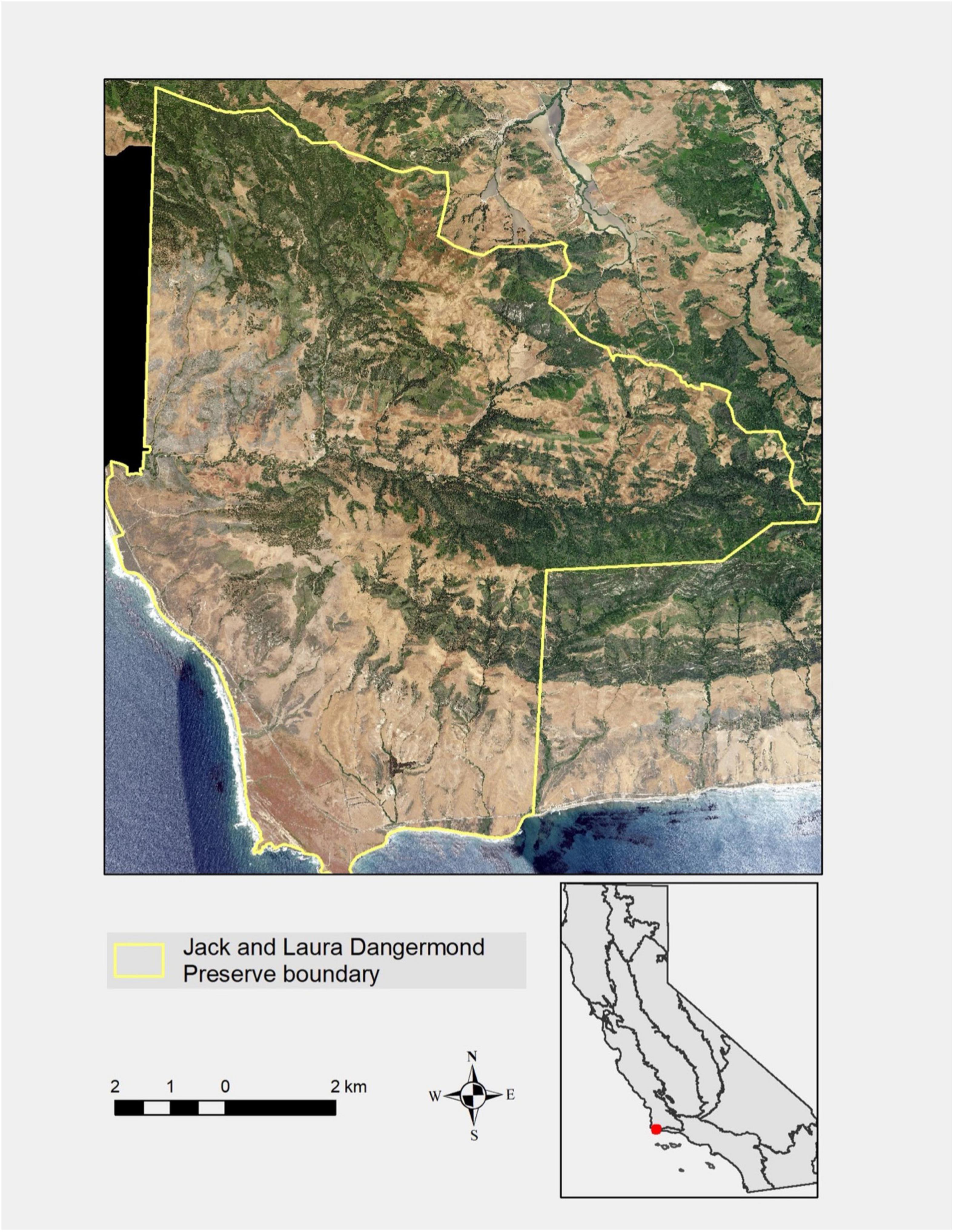
Figure 1. Location map showing California floristic region boundaries, and 2020 orthophoto of the Jack and Laura Dangermond Preserve (JLDP, N 34.49°, W 120.44°). Shrublands and oak forests are dark green and grasslands are brown in this image.
The area supports a mosaic of grassland, shrubland, woodland, and forest communities that reflect underlying diversity in topography, climate, geology, and soils. Here we focus on the JLDP’s coast live oak (Q. agrifolia) forest and woodlands. Coast live oak is an evergreen red oak that is widespread in the region, often dominating closed forests, open woodlands, and savanna with grass or shrub-dominated understories (Callaway and Davis, 1998). Vegetation classified as coast live oak forest and woodlands is characterized by >20% tree cover and greater than 50% relative tree cover of Q. agrifolia, per class definitions based on the Manual of California Vegetation (Sawyer et al., 2009). Based on recent detailed mapping, coast live oak woodlands occupy 2,440 ha or 25% of the preserve area (WRA Inc, 2017; Figure 2).
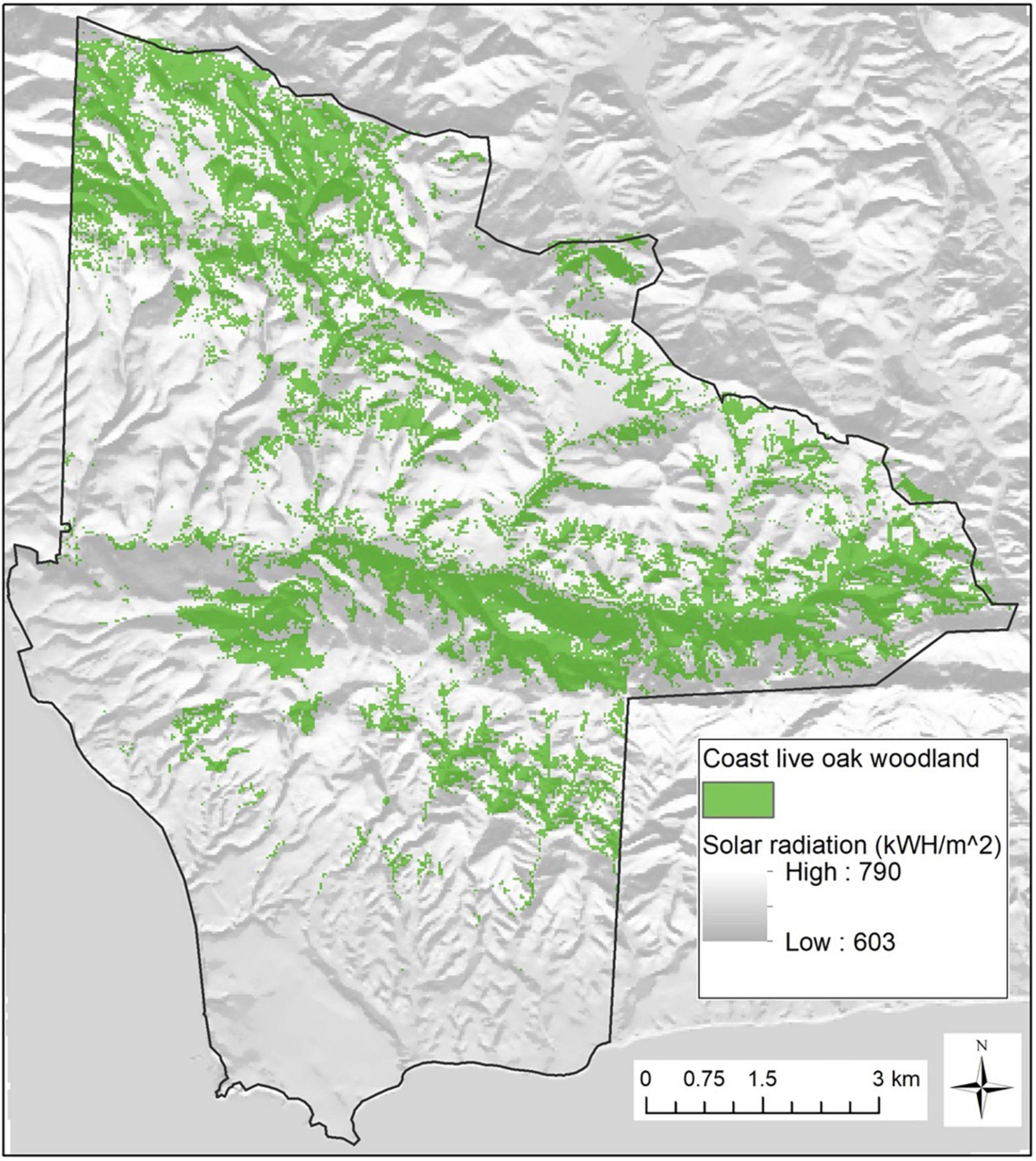
Figure 2. Map of coast live oak (Quercus agrifolia) woodlands on the preserve superimposed on modeled December–June (solstice-to-solstice) solar radiation (kWH/m2). Grid resolution of the woodland mask is 30 m and solar radiation is computed from a 10 m digital elevation model.
Elevations at JLDP range from sea level to 645 meters above mean sea level (mamsl), and oak woodlands occur from roughly 15–520 mamsl. Rugged topography produces large spatial variation in solar radiation load and surface hydrology (Figure 2). Modeled JLDP-wide annual temperature for the period 1971–2000 averaged 13.2°C, but thermal regimes vary with elevation and distance from the coast (Flint and Flint, 2012). The coastal zone is under a strong marine inversion layer with summer base height typically 250–400 mamsl, and frequently experiences morning fog and relatively cool temperatures during summer months compared to more inland areas and areas above the marine boundary layer (Dorman and Winant, 2000; Supplementary Figure 1).
Annual rainfall averages 46.7 cm between November and April, increasing at higher elevations in the northwest and central portions of the preserve (Supplementary Figure 2). The ratio of precipitation to potential evapotranspiration (aridity index) is higher (i.e., more mesic) in these same areas (Figure 3).
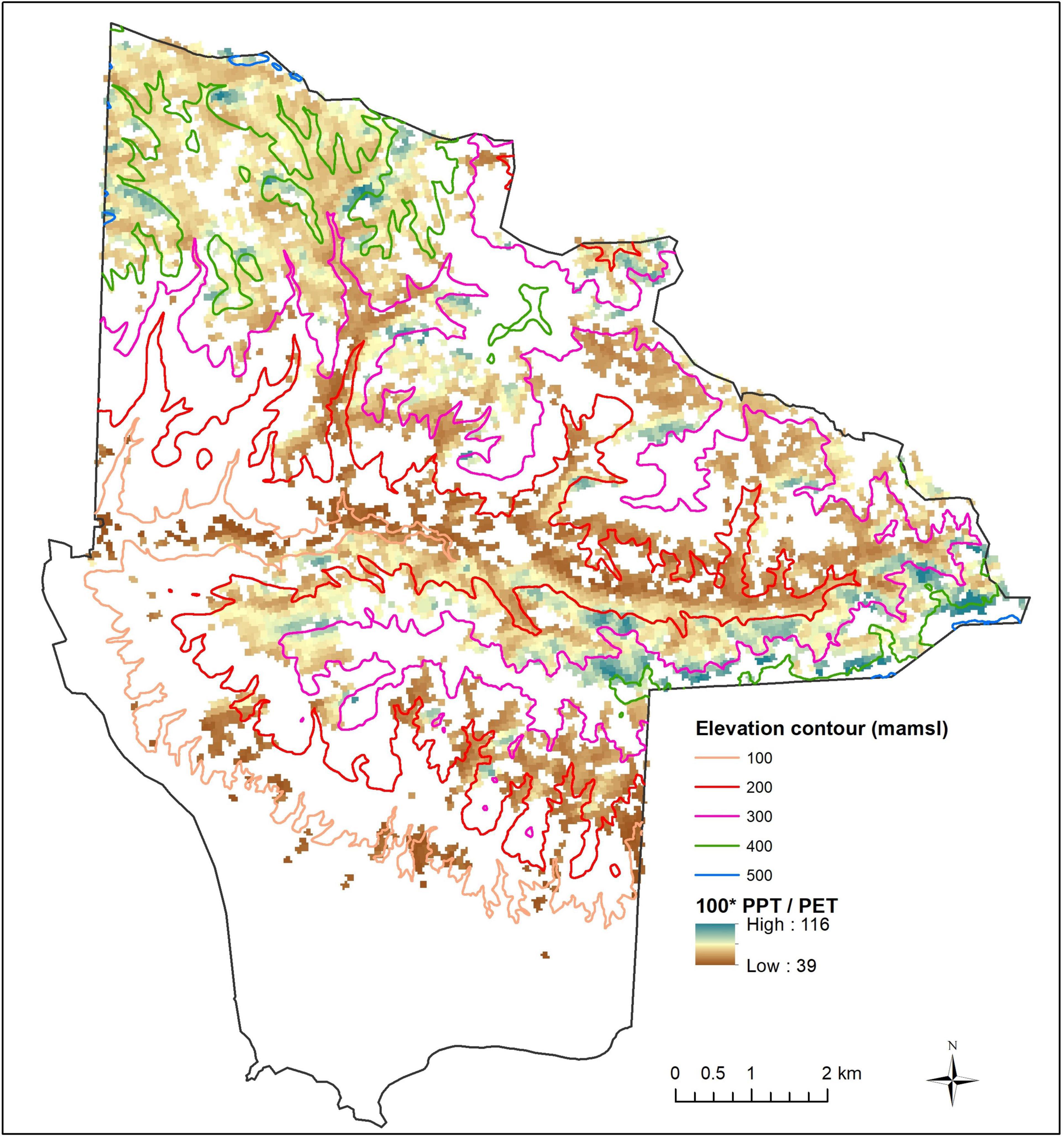
Figure 3. Modeled mean aridity index (100 × annual precipitation/annual potential evapotranspiration) for the period 1971–2000 at 90 m resolution. Driest areas (brown) are preferentially distributed toward lower elevations.
Surficial geology and soils can exert a strong control on distributions of tree and shrub species in the region (Wells, 1962). Dibblee (1950) mapped 26 geologic formations or sub-formations on JLDP, but 92% of coast live oak woodlands occur on only 11 units and 70% occur on four geologic formations: Monterey shale, Matillija sandstone, Jalama micaceous shale, and Anita shale (Figure 4). Much of the Monterey formation is mantled by moderately deep, well drained, acidic, shaly-loam soils of the Santa Lucia series and Lopez-Santa Lucia complex. The shallow, well-to-excessively drained Gaviota sandy loam and San Andreas coarse sandy loam soil series are widespread on Matillija, Jalama, and Anita geologic formations (Shipman, 1981; Supplementary Figure 3).
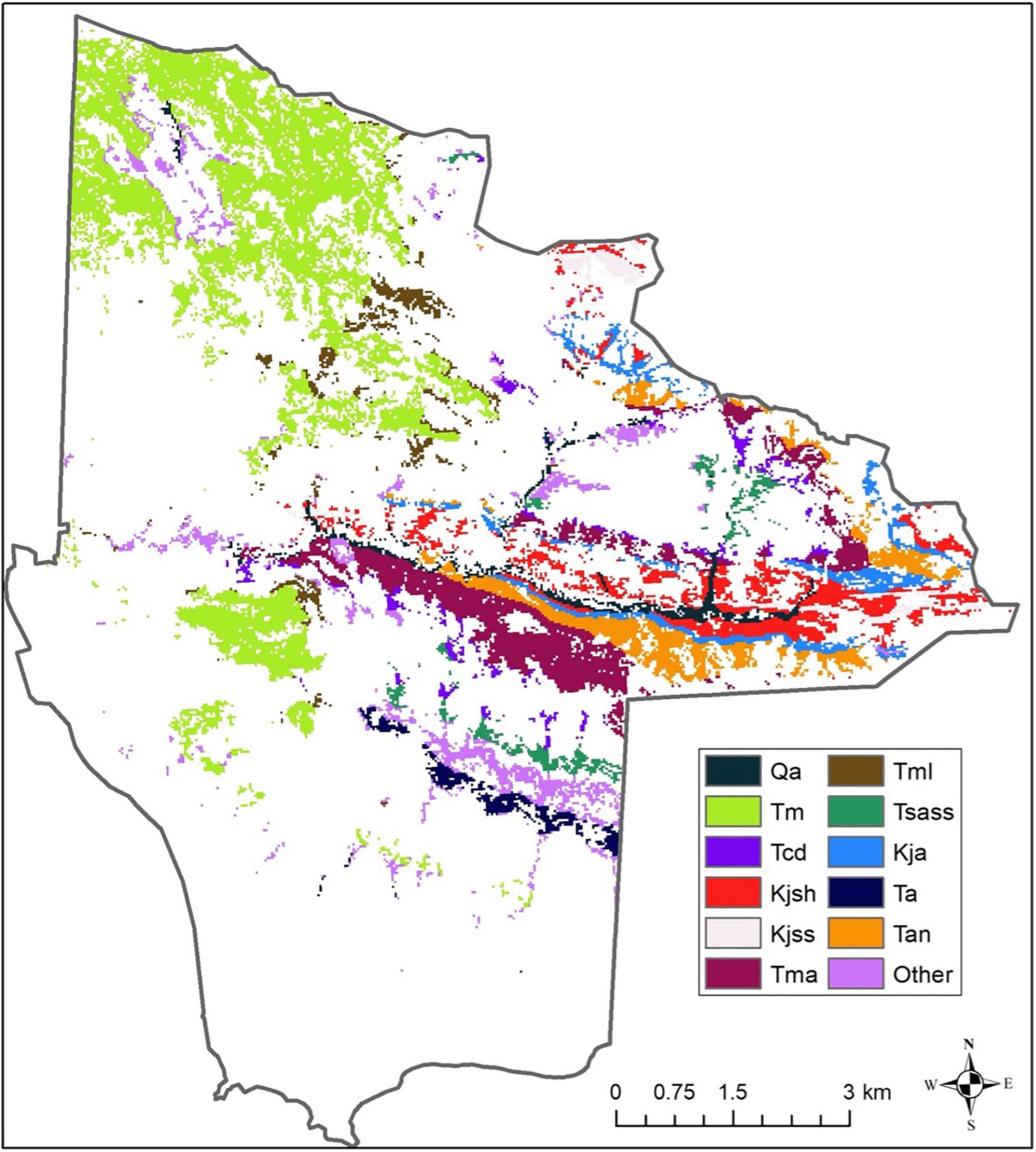
Figure 4. Geology underlying mapped oak woodlands. Formation codes: Cretaceous (K), Quaternary (Q), Tertiary (T), alluvium (Qa), Monterey shale (Tm), Cozy Dell micaceous shale (Tcd), Jalama micaceous shale (Kjsh), Jalama sandstone and siltstone (Kjss), Matillija sandstone (Tma), Monterey shale lower siliceous shale (Tml), Sacate sandstone and shale (Tsass), Jalama sandstone (Tja), Allegria formation (Ta), Anita shale (Tan).
Based on available fire perimeter data the eastern portion of JLDP has been fire-free since at least 1950. Shrublands in the northwestern portion of the preserve experienced prescribed burns designed to increase forage production associated with cattle operations (i.e., range improvement) in 1981, 1998, and 2000 (Supplementary Figure 4). Wildfires spread into the western portion of JLDP in 1981, 2002, and 2004 (Supplementary Figure 5). The 1981 wildfire perimeter encompassed 234 ha of oak woodland; the 2002 and 2004 wildfire perimeters encompassed 18 and 1 ha of oak woodland, respectively.
Like most of California, JLDP experienced extreme drought between 2012 and 2016 and generally droughty conditions from 2012–2019. Statewide, the drought severely impacted water supply, forage production, and woody plant health and survival (Lund et al., 2018; Warter et al., 2021). Elevated, drought-induced tree water stress and mortality were documented for oak and conifer species in many regions of California (e.g., Asner et al., 2016; Das et al., 2020) and were also observed but until this study not formally analyzed at the preserve.
To produce an ecological land classification for JLDP we analyzed L45 Collection 2 Level-2 imagery (Table 1), including 134 images acquired between November 1982 and December 2000. Relative to Landsat Collection 1, Collection 2 data feature substantially improved absolute geolocation, as well as cloud-optimized GeoTIFF format and globally available Level-2 surface reflectance and surface temperature products (Wulder et al., 2019).
To test the ecological land classification, we analyzed 169 HLS surface reflectance images acquired between April 2013 and December 2020. HLS merges Landsat 8 with the European Space Agency’s Sentinel-2 constellation to provide a single intercalibrated multispectral image archive at 30 m resolution (Masek et al., 2018). Data streams are atmospherically corrected, spatially co-registered, BRDF (bidirectional reflectance distribution function) normalized, and bandpass adjusted to provide a single data stream achieving roughly 3–5 days global revisit since the 2017 launch of Sentinel-2b.
Remote sensing analysis for both L45 and HLS imagery was performed in three steps. In the first step, linear spectral mixture analysis (SMA) was applied to each cloud-free image. For each pixel in a multispectral image, SMA estimates the areal fractions of a small number of spectral endmembers (sEMs) (Adams et al., 1986; Gillespie, 1990; Smith et al., 1990). We used a set of three generalized sEMs specific to L45 and three sEMs specific to HLS that represent: (1) soil and non-photosynthetic vegetation substrates; (2) illuminated photosynthetic vegetation (V-fraction); and (3) dark targets like shadow and water. Analyses of diverse compilations of Landsat images have shown that these three generic sEMs mix linearly to characterize the vast majority of terrestrial surfaces (Small, 2004; Small and Milesi, 2013). Both sets of sEMs used here were based on extensive, previously published analyses: the 1982–2000 Landsat sEMs from Sousa and Small (2017) and the 2013–2020 HLS sEMs from Small (2018).
In the second step, cloud-free V fraction images were compiled into image time series and unmixed using a linear temporal mixture model (TMM) approach (Quarmby et al., 1992; Piwowar et al., 1998; Lobell and Asner, 2004). We apply the specific approach described in Sousa and Davis (2020): briefly, a Mediterranean-climate oak landscape is considered a mixture of evergreen perennial, deciduous perennial, annual herbaceous, and unvegetated temporal endmembers (tEMs). Conceptually, considering a multitemporal V fraction pixel as a linear mixture of tEMs is analogous to considering a one-time multispectral pixel as a linear mixture of sEMs.
In the third step, we examined drought impacts on oak woodlands by applying a novel technique of TMM residual analysis. We extended the approach of mixture residual analysis from the spectral domain to the temporal domain (Sousa et al., 2022). Conceptually, this asked the question: What residual temporal signal observed in the V fraction time series is not accurately modeled by a least squares solution of decadally stable tEMs? This question can be addressed by computing the difference between the observed V fraction time series and a modeled V fraction time series based on linear combinations of tEMs alone. HLS TMM residual time series (TMRs) were calculated for each oak woodland pixel. The first three principal component scores of the TMR time series (TMR1, TMR2, and TMR3) were used to assess spatial patterns of vegetation change from 2013 to 2020.
The theoretical basis for the temporal mixture residual approach was conceived as follows:
1. In theory, pixels with interannually stable vegetation phenologies should be well-represented by a simple linear mixture of tEMs. Such stable areas should be characterized by low mixture model misfit and near-zero TMR time series.
2. In contrast, pixels with interannually unstable vegetation phenologies – here, areas subject to drought-associated oak dieback – should be poorly represented by a simple linear mixture of tEMs. Such unstable areas should be characterized by high mixture model misfit and large TMR time series amplitudes. Because the TMR gives temporally explicit account of this misfit, fidelity is retained in capturing both progressive and abrupt changes.
3. The low-order principal components of the TMR time series should provide a concise characterization of the major spatiotemporal patterns of deviation from the linear TMM. To the extent that oak dieback is the major multi-year, landscape-scale vegetation change within the study area, it should be well represented in the low-order TMR dimensions (e.g., 1, 2, and 3).
To calibrate TMR scores against oak canopy cover change between 2013 and 2020 we quantified live tree canopy cover in National Agriculture Imagery Program (NAIP) digital orthophotos acquired on 5 May 2012 and 7 June 2020. The 2020 image was resampled from 60 cm to 1 m resolution to be consistent with the resolution of the 2012 image. Eighty sample sites were distributed evenly among decile classes of the TMR1 scores. Samples were confined to mapped oak woodlands and to TMR1 decile “patches” at least 60 × 60 m in extent to avoid isolated and edge pixels. We overlaid 25 points in a 5 × 5 10 m grid array over the sample area and visually assigned each intercepted point location in the photo to 1 of 3 classes: (1) live tree canopy, (2) not live tree canopy, and (3) shadow that was too dark to assign the point to Class 1 or 2. Percent live tree canopy in each sample site was calculated as:
where Cy is % live canopy in year y, n1 is the number of points in Class 1, and n3 is the number of points in Class 3. Oak cover change from 2012 to 2020 (C1220) was calculated as C2020 – C2012. Canopy change was related to TMR scores by simple linear regression using the R base function lm (R Core Team, 2019). Given moderately high test sample linear correlation between TMR dimensions 1–3 (r = 0.50–0.59), the final calibration was produced using only TMR1.
We note that in theory this approach could yield a direct estimate of canopy dieback from aerial imagery alone – if enough aerial imagery were available to provide repeat coverage of all relevant oak landscapes, and if enough analyst time were available to do the manual estimation of canopy change. The value of the Landsat-based approach is that it can be automated for any relevant oak landscape on Earth, going back to the 1980s, and can also provide temporally explicit information about the onset, rate, and duration of dieback events.
Gridded GIS variables were all resampled to 30 m resolution to match the spatial resolution and map projection of the L45 and HLS imagery. We chose a limited set of bioclimatic and edaphic variables for ecological land classification that are known to influence Q. agrifolia distribution and dynamics in the region and that were mapped with sufficient reliability and at an appropriate scale for landscape analysis. These included three bioclimatic factors, two topoclimatic factors, and five edaphic factors (Table 1). While 10 variables may seem manageable at first glance, note that combinatorial explosion – e.g., as recognized decades ago in physical chemistry and metabolomics (Morowitz et al., 2000; Schuster, 2000) – nevertheless results in a deep parameter space with a vast number of possible thresholds and inter-variable interactions.
Bioclimatic variables included mean annual precipitation (MAP), average maximum daily temperature of the warmest month (TMAX, a proxy for marine layer influence), and aridity index (ARID, calculated as 100 × MAP/PET, where PET is modeled potential evapotranspiration). MAP, TMAX, and ARID for the period 1971–2000 were extracted from statewide 90 m grids and oversampled to 30 m using bilinear interpolation. The statewide grids were initially produced by downscaling 4 km PRISM grids (Daly et al., 2008) using spatial Gradient and Inverse Distance Squared weighting (GIDS) as described in Flint and Flint (2012) and Franklin et al. (2013).
Topoclimatic variables included solar radiation (SOLAR) and hillslope flow accumulation (FLOW). Integrated December–June (winter to summer solstices) solar radiation was calculated in ArcGIS using a 10 m digital elevation model (DEM) (Fu and Rich, 2002; Figure 2). The 10 m DEM was also used to model flow accumulation in ArcGIS. We weighted a cell’s contribution to the contributing area by tan(slope). Solar radiation and flow accumulation grids were re-sampled to 30 m using bilinear interpolation. Flow accumulation was then log10 transformed prior to analysis (Supplementary Figure 6).
Surficial geology (GEOL) was simplified to 11 classes that underly 92% of JLDP oak woodlands. Remaining areas were lumped into “Other Geology” (Figure 4). Mapped soil series (SOIL) were similarly simplified to 12 series covering 92% of oak woodlands, plus a 13th group for all other series (Supplementary Figure 3). We also analyzed the tabulated physical and chemical soil properties for all series, including percent sand fraction (PSAND), percent clay fraction (PCLAY), and pH (pH).
Grids of areas mapped as wildfires or prescribed fires based on 1980–2020 fire perimeter data from CalFire1 were coded based on the year of the fire event, and treated as categorical variables in the land classification analysis. For example, a cell could have one of four values for wildfire: not burned, burned in 1981, burned in 2002, or burned in 2004. For prescribed burns, a cell was coded as not burned, burned in 1981, burned in 1998, or burned in 2000.
All 30 m oak woodland pixels with values for all variables (co-registration edge effects led to missing values for some variables) were included in the analysis (n = 17,788 spatial pixels).
All statistical analyses were conducted using R v. 3.6.1 (R Core Team, 2019). We conducted initial exploratory analyses with Random Forest (R package randomForest v. 4.6-14) to identify potentially important variables for predicting spatiotemporal variation in canopy cover in the 1981–2000 L45 imagery (Breiman, 2001). Based on model pseudo-R2, we set the number of trees grown to 500 and randomly sampled three predictor variables at each split of the tree. We examined the relationship between tree size and model fit – measured as variance explained – for tree sizes ranging from 2 nodes to 20 nodes. We also produced variable importance plots to evaluate which environmental factors were consistently influential for parsimonious tree sizes.
A final ecological land classification was produced by multivariate regression tree analysis of the first three principal components of the temporal feature space of the L45 V fraction time series using the R package mvpart 1.6-2 (Larsen and Speckman, 2004; De’ath, 2014). Multivariate regression trees are an extension of regression tree analysis from a single dependent variable to multiple dependent variables (Larsen and Speckman, 2004). At each node of the tree, multivariate analysis of variance is used to select the splitting variable that best partitions total variance in the dependent variables. Large trees were produced and then pruned back to only those splits that explained at least 2% of starting variance. The resulting stratification was applied to GIS data layers to map oak woodland land classes on the preserve.
We tested the association of L45-derived land classes with HLS imagery by measuring the percent of variance in HLS TMR 1–3 that was explained by the land classification. For comparative purposes we also undertook the same random forest and multivariate regression tree analysis performed on the first three principal components of the L45 V fraction time series to the first three principal components of the HLS V fraction time series.
We measured association between HLS TMR1, TMR2, and TMR3 scores and environmental factors using Pearson’s product moment correlation (r) and analysis of variance. We evaluated the skill of the ecological land classification for partitioning oak canopy change from 2013 to 2020 by analyzing variance in TMR1 scores and estimated C1220 values at sequential splits in the multivariate classification tree and for the tree as a whole.
As described in section “Materials and Methods,” we analyzed statistical derivatives from two distinct image time series: the 2000–2011 Landsat 4–5 Thematic Mapper dataset (L45) and the 2013–2020 HLS dataset. For each time series, we computed both: (a) the principal components (PCs 1–3) of the vegetation fraction time series, and (b) the PCs of the temporal mixture model residual (TMRs 1–3). The first three principal components explained over 85% of variance in both L45 and HLS time series. For both L45 and HLS imagery, spatial patterns of PCs 1–3 revealed broad differences between oak woodlands in northwestern or southern compared to central-eastern regions of JLDP (Figures 5A,B). The dominant modes of variability were evergreen canopy cover (PC1 in both cases) and seasonal greening with a peak in springtime and decreasing green canopy cover throughout the remainder of the calendar year (combination of PC2 and PC3 in both cases). Topographic variability was also observed, presumably driven by a combination of real, solar radiation-driven variability in vegetation structure and composition along with artifacts associated with illumination and sun-sensor geometry that persisted despite topographic and BRDF correction.
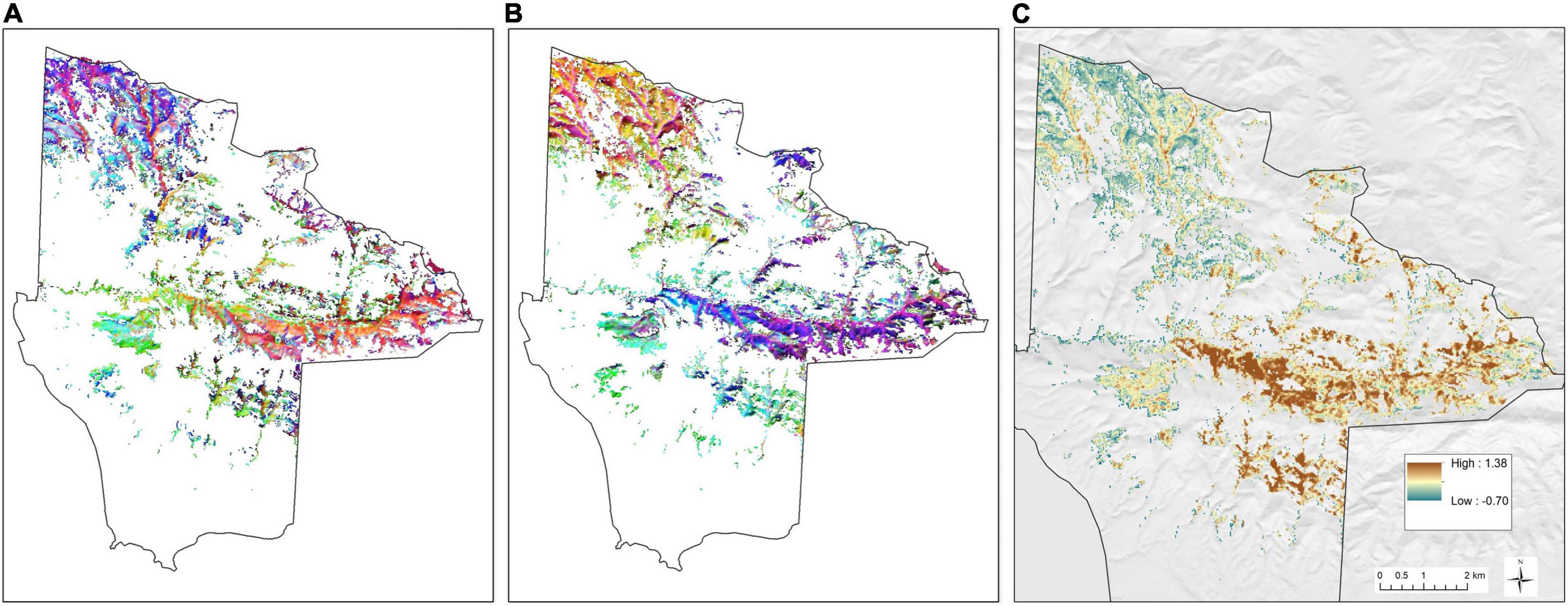
Figure 5. Principal component images. Panels (A,B) show false color composites where PC 1, 2, and 3 correspond to the red, green, and blue channels of each image. Panel (A) shows PC results for Landsat 4/5 (2000–2011) and panel (B) shows HLS (2013–2020). Panel (C) shows the first principal component only of the HLS temporal mixture residual (TMR1).
The spatial pattern of the TMR scores was similar to patterns in the L45 and HLS TMMs (Figure 5C), but upon close inspection, mixture residuals exhibited less topographically related variation and more spatially coherent local neighborhoods – particularly in the central-eastern region where large contiguous areas form an east-west belt of high TMR1 scores (Figure 5C). This belt is underlain by Matillija sandstone, Anita shale, Gaviota sandstone, and Allegria sandstone. Much of this area is mapped as Gaviota sandy loam soil.
The temporal trajectory of image mean TMR scores reveals the JLDP-wide trend in evergreen canopy cover during the multi-year drought. TMR1 scores decline steeply between 2014 and 2016, then more gradually from 2016 to 2017 before leveling off from 2018 to 2020 (Figure 6). In contrast, the average trajectory for TMR2 decreased slightly from 2013 to 2015 and then increased from 2016 to 2020 (Figure 6). The trajectory for TMR3 remained relatively flat from 2014 to 2020 (Figure 6). TMR1 is negatively correlated with MAP (r = −0.44), TMAX (r = −0.39), and ARID (r = −0.23) and only weakly correlated with SOLAR, FLOW, and soil physical or chemical properties (|r| < 0.05) (Table 2).
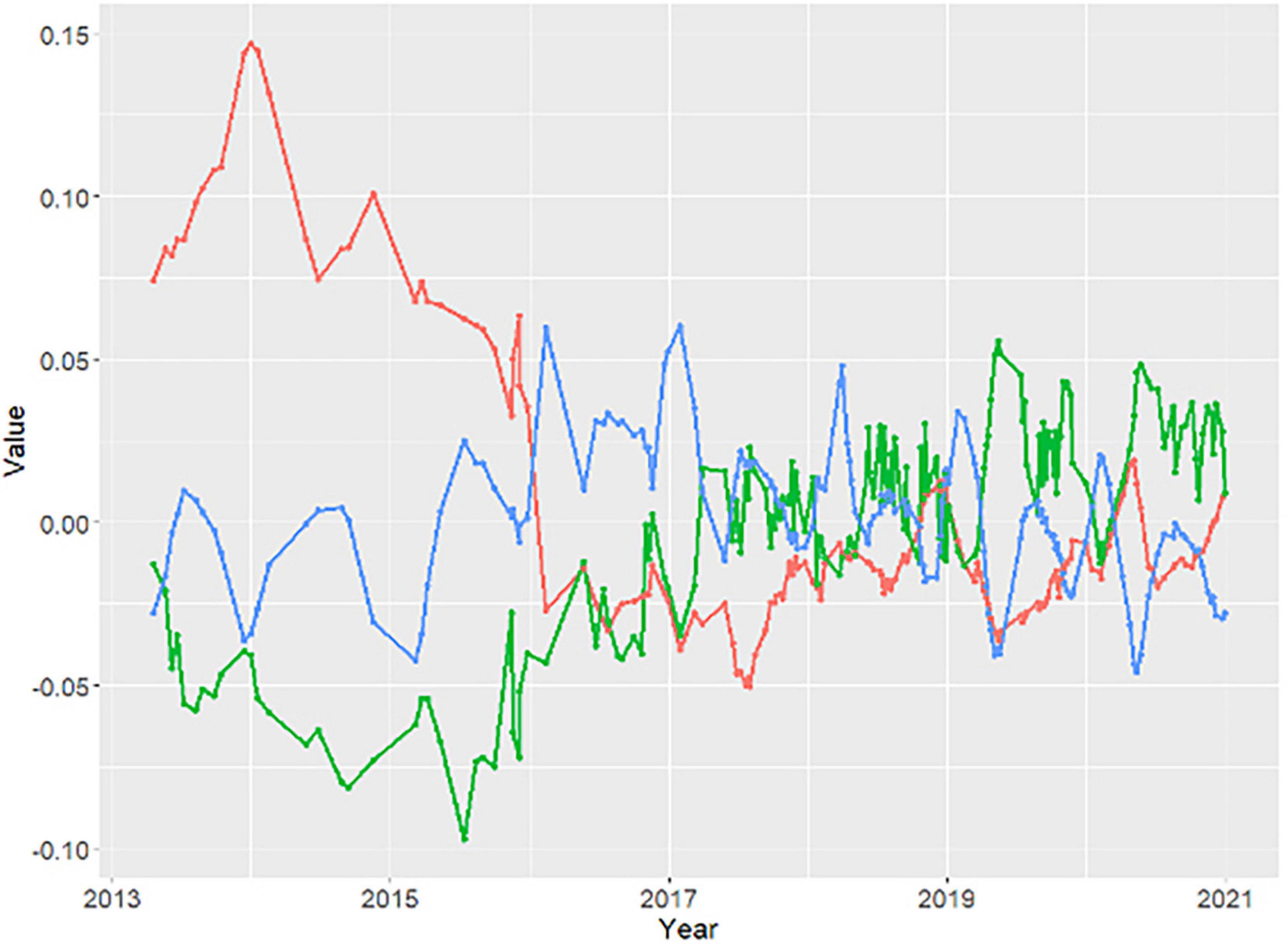
Figure 6. Time series of dominant spatiotemporal patterns in the temporal mixture residual (red, TMR1; green, TMR2; blue, TMR3). Note variations in both timing and amplitude of temporal mixture model misfit, with largest changes coinciding with severe drought years (2013–2016).
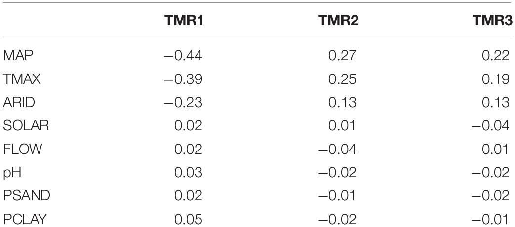
Table 2. Correlation of HLS temporal mixture model residual (TMR) scores with continuous bioclimatic and soil properties.
Based on air photo analysis, TMR1 is a good proxy for oak canopy change from 2012 to 2020, explaining 74% of the variance in observed oak canopy change in 2012–2020 air photos (Figure 7). Each 0.1 increase in TMR1 represents an estimated 4.8% decrease in live oak canopy over the 8-year interval (C1220 = 9.23−48.35 × TMR1, degrees of freedom = 78, adj. r2 = 0.738, p << 0.001).
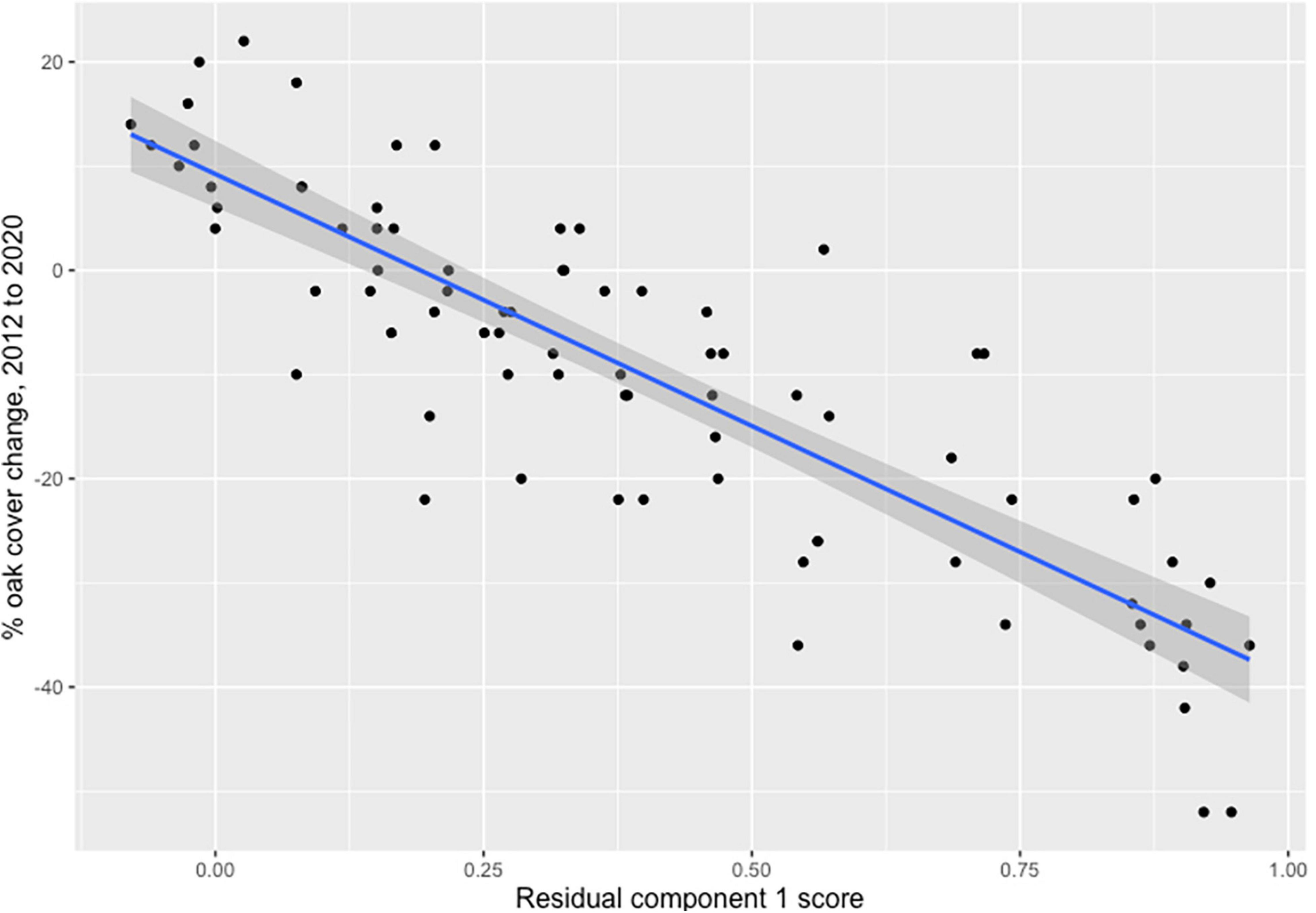
Figure 7. Scatterplot of oak canopy change from 2012 to 2020 (C1220) vs. TMR1 scores based on analysis of 80 sample sites in May 2012 and June 2020 digital orthophotos. The fitted regression model is: C1220 = 9.23–48.35 ×TMR1. Adj. r2 = 0.74, p << 0.01.
Random forest and univariate regression tree analyses of the first three principal components of L45 TMM scores are summarized in Supplementary Tables 1, 2. Overall, small trees (4–5 nodes) captured 22–33% of the variance in each of the L45 TMM principal components. Trees of larger sizes yielded only minor incremental gains in model performance (Supplementary Figures 7–9). The most important model variables were the same for random forest and regression tree models: SOLAR, GEOL, SOIL, ARID, and TMAX. Fire history variables were consistently of low importance. Roughly equivalent variance was explained by random forest models and pruned regression trees of the same size.
Multivariate regression tree analysis yields a 5-node tree that explains 22.5% of the total variance in the first three L45 TMM principal components (Figure 8). Oak woodland sites are partitioned into high and low solar radiation classes and two groups of geologic formations. Classes 1, 2, and 4 are dominated by Monterey shale (Tm) and located mainly in the northwestern and southern parts of JLDP, while Classes 3 and 5 are dominated by Matillija sandstone (Tma), Jalama micaceous shale (Kjsh), and Anita shale (Tan) and form an east-west belt in the central and eastern parts of JLDP (Figure 9). Classes 1 and 2 are separated based on aridity (Figure 8). The spatial pattern of these five classes across the preserve shows obvious similarity to patterns in the L45 TMM scores as well as to HLS TMM scores and HLS TMR1 scores (cf. Figures 5, 9).
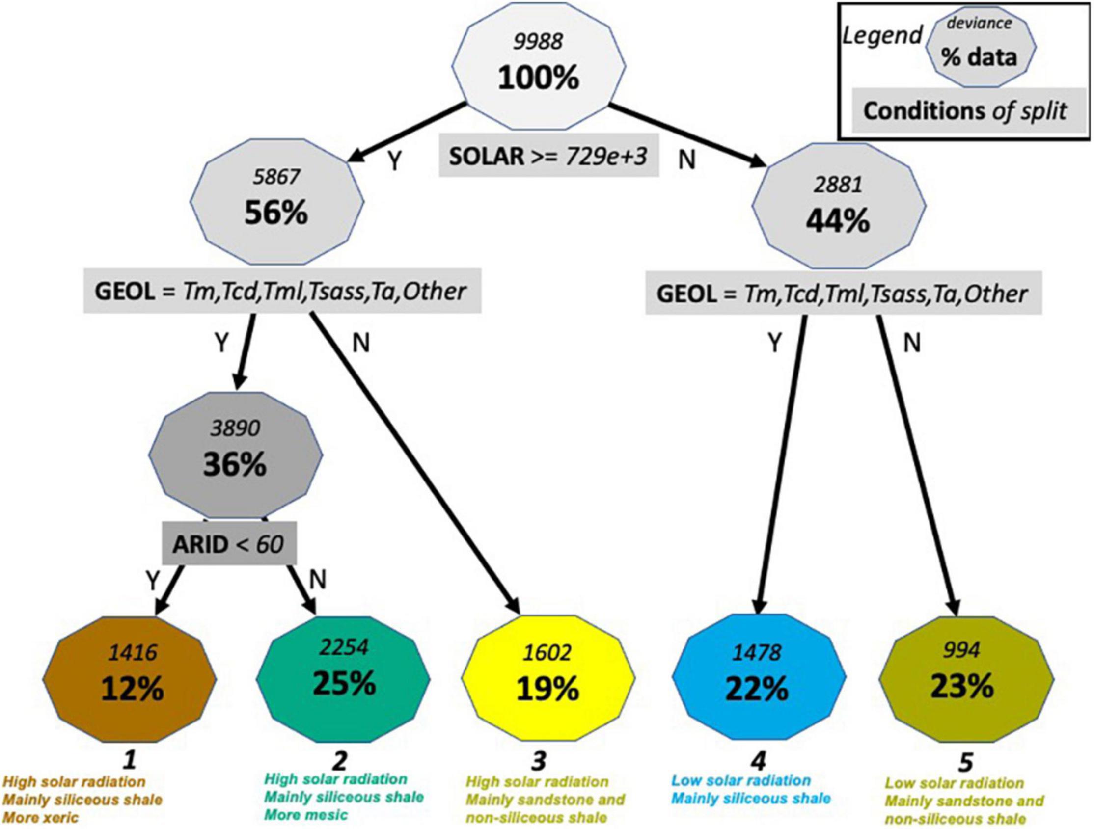
Figure 8. Multivariate regression tree for the first three principal components from temporal mixture modeling of L45 imagery, 1982–2000. Numbers in the blue boxes are total deviance and percent of the starting sample (n = 17,788). Splitting criteria are in the green boxes. At each split, subsets to the left meet the criterion (Y) and those to the right do not (N). See Table 1 for explanation of variables and acronyms. Bold numbers at the bottom correspond to class numbers in Figure 9.
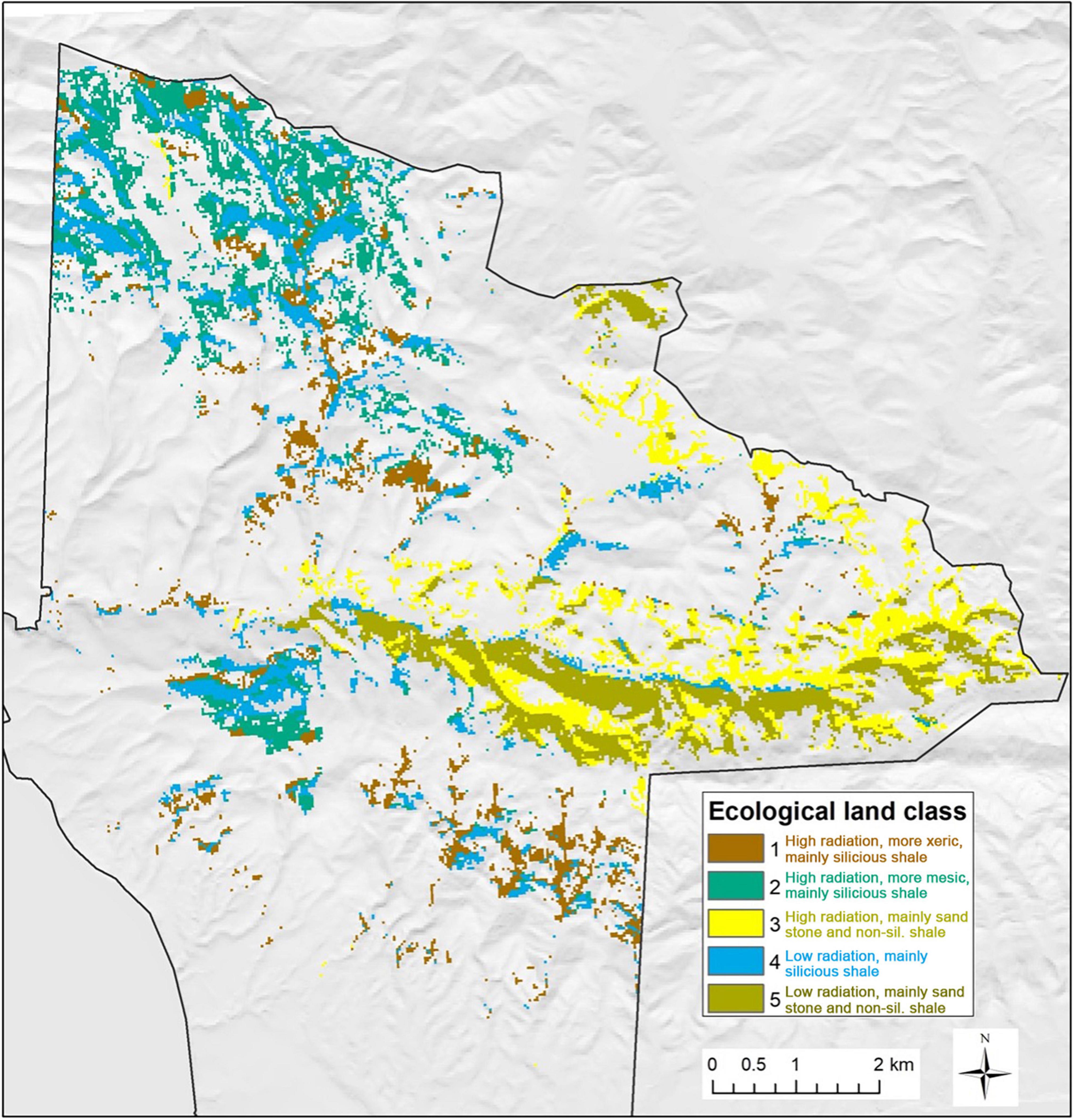
Figure 9. Ecological land classes for areas currently occupied by coast live oak woodland at the preserve. Class numbers refer to terminal nodes in the classification tree shown in Figure 8.
The five land classes based on 1982–2000 L45 imagery explain as much or more of the variance in the 2013–2020 HLS TMM PC images (Table 3). The stratification is also relatively effective at partitioning variance in TMR1 scores (27%), less so with TMR2 (4.9%), and TMR3 (12.8%).
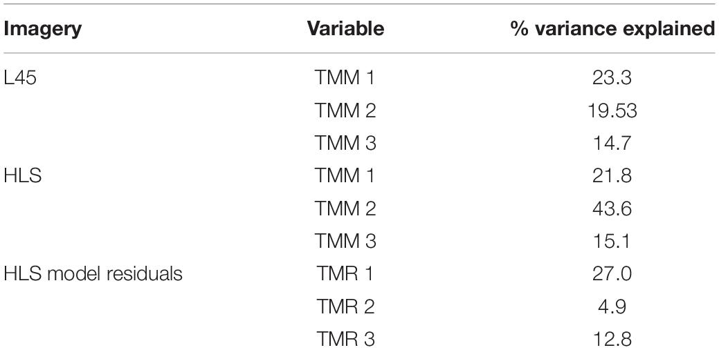
Table 3. Image variance explained by the 5-class land stratification derived from Landsat imagery, 1980–2000.
Random forest models capture 27–50% of the variance in HLS TMM PCs 1–3. As with the models based on L45 imagery, SOLAR, GEOL, SOIL, ARID, and TMAX are the most influential variables, along with MAP, in predicting TMM PC scores. Fire history is relatively unimportant. Similarly, 3–4 node regression trees based on SOLAR, soil factors, and ARID account for 38–48% of variance in HLS TMM PCs 1–3. FLOW also appears as an important variable for predicting HLS TMM3 scores.
Surficial geology, SOIL, MAP, and TMAX also prove most important in random forest and regression tree models predicting TMR scores (Supplementary Tables 1, 2). A 4-node tree based on SOIL, pH, and MAP explains 36% of the variance in HLS TMR1 scores.
As noted above, stratifying HLS TMR1 scores by land classes accounts for 27% of the variance in the scores. Mean scores for Classes 1, 3, and 5 are relatively high (0.41, 0.52, and 0.46, respectively) compared to Classes 2 and 4 (0.24 and 0.25) (Figure 10). Based on the linear relationship to oak canopy cover change (Figure 7), this equates to an average reduction in live oak canopy of 10–16% in Classes 1, 3, and 5 between 2012 and 2020 compared to a 2–3% decline in Classes 2–4. These differences are not related to solar radiation, as the first split of the tree into high and solar radiation classes explains less than 0.1% of total variance. Instead, the association of TMR1 score and land classes is due to subsequent splits by geology and aridity.
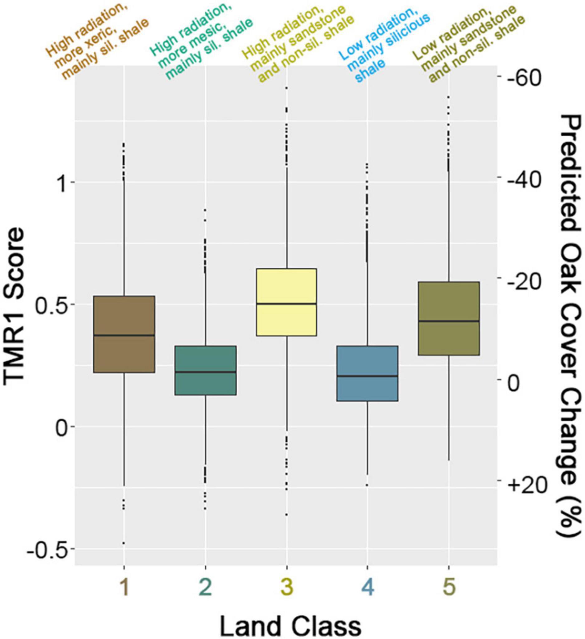
Figure 10. Boxplots of TMR1 scores split by five ecological land classes identified by multivariate regression tree analysis of L45 TMM imagery. The right axis shows the predicted change in percent oak canopy cover from 2012 to 2020 based on linear regression (cf. Figure 7).
Ecological land classifications are produced for various purposes such as sample stratification, ecosystem inventory and mapping, environmental planning and impact assessment. Whether based on expert opinion or multivariate statistics, classification analyses are best undertaken for exploration or prediction, rather than for inference about ecological processes. Although land classifications should be grounded in ecological theory and knowledge (Rowe and Sheard, 1981), it is not appropriate to assign a causal or mechanistic basis to land classes. A classification scheme is purpose-driven and successful to the extent that it is predictive of variation in ecological attributes or processes of interest across the landscape. The classification produced here using 1982–2000 L45 imagery demonstrated predictive utility in distinguishing areas of the preserve where oak woodlands have similar defining features (geology, soils, and topoclimate) and manifested significantly different impacts from severe drought that occurred between 2012 and 2020.
Our case study focused on classifying coast live oak woodland sites for sampling, monitoring, and siting restoration experiments. As is often the case, predictor environmental variables co-varied spatially, making it difficult to single out any one factor controlling oak woodland changes through time. Such co-variation should contribute to a more robust stratification than one based on a single factor, particularly as that co-variation occurs at site-to-landscape spatial and temporal scales.
The ecological land classes differed systematically in the extent of drought-associated oak canopy dieback. Our hypothesis is that this reflects systematic class differences in rooting-zone water availability. This could be tested by monitoring plant water status (i.e., pre-dawn Xylem Pressure Potential) for oaks in different land classes during extreme drought vs. non-drought water years. A second hypothesis is that class differences in oak canopy dynamics will also be manifested as class differences in associated understory plant community composition. This could be tested by class-stratified sampling of plant community species composition, functional trait diversity, and structure.
Our analysis also revealed areas (Classes 2 and 4) that showed little or no drought impact. Restoration could focus on sites with similar environmental properties where oak canopy has been reduced by historical clearing. Those areas would bet-hedge against future warming trends and drought episodes. Our analysis also revealed areas with high oak canopy loss (Classes 1, 3, and 5). Those areas would appear to be good candidates for restoration based on historical conditions, but would be more vulnerable to future warming and episodes of extreme drought.
Recent fire history also co-varied with edaphic and bioclimatic variables but, somewhat surprisingly, was not influential in most of the random forest or regression tree models or in the final land classification. This may be because fires were incompletely mapped, because mapped fires had only minor impacts in coast live oak woodlands, and/or because fire effects in oak woodlands occurred at a finer scale than could be represented with fire perimeter data. This highlights the point that we did not formally address the issue of spatial scale-dependence in our analysis. Research is underway to test how well the approach used here performs across larger spatial extents or with finer- or coarser-grain terrain data or satellite imagery.
Topographic, edaphic and bioclimatic controls on coast live oak distribution and cover have been previously documented for central coastal California, and the influence of these variables in the random forest and regression tree models is consistent with what is known about the species’ environmental associations. Although coast live oak occurs on a wide variety of substrates in many settings, the species reaches relatively high cover regionally on specific rock types such as the siliceous shale of the Monterey Formation (Wells, 1962) and the arkosic sandstone of the Matillija and Gaviota Formations (Callaway and Davis, 1993). At finer scales, oak cover increases on slopes with lower solar radiation loads and on lower footslopes and riparian habitats (Davis and Goetz, 1990).
Less well understood is how coast live oak population and canopy dynamics differ within and between landscapes as a function of site properties. At the Dangermond Preserve we observed areas of extensive dieback of coast live oak between 2012 and 2020 almost certainly related to a multi-year severe drought event (but see Chacon et al., 2020). We documented pronounced, systematic differences in coast live oak canopy trends on different sites. The strong association of canopy dynamics with surficial geology and soils suggests that differences in subsurface water storage capacity as well as precipitation input could have played a role in the extensive oak dieback in some areas and stable or increasing canopy in others (e.g., Hahm et al., 2019). McLaughlin et al. (2020) observed variation in blue oak (Quercus douglasii) mortality during the 2012–2016 drought related to bedrock lithology as well as to variation along hillslope hydrologic gradients. The land classification derived here could be useful to designing future ecohydrological studies to assess differential vulnerability of coast live oak populations to projected warmer drier conditions under 21st century climate change. It could also help to direct restoration efforts (e.g., away from areas that appear especially sensitive to extreme drought).
Solar radiation is a primary variable in the land classification, but oak canopy trends during the drought event were not obviously related to local solar radiation load. In heavily impacted areas, dieback and mortality appear to be as likely on north-facing slopes – and on lower hillslopes with higher modeled flow accumulation – as on other topo-facets. Both solar radiation and flow accumulation can only be approximated with DEMs and the algorithms used here, so additional ground surveys would be required to confirm this result.
Ecological land facets have been advocated for conservation planning and decision making in the face of climate change (e.g., Anderson and Ferree, 2010; Beier and Brost, 2010). Challenges with this approach include the relative importance of biotic vs. abiotic drivers of species distributions and dynamics, spatial and temporal scale-dependence, as well as spatial and temporal variation in the relationship between landforms and local climate conditions (Lawler et al., 2015). In areas lacking detailed ground surveys and monitoring, land classification using long-baseline satellite imagery may contribute to a refined definition of, and operational approach to, mapping and monitoring landscape-specific land facets.
Imagery-guided land classification may also support mapping and monitoring of local climate refugia (Hannah et al., 2014). Refugium identification and protection is of obvious importance for 21st century environmental conservation, but often necessarily relies on indirect landscape cues due to absence of detailed historical records. The duration of the Landsat archive may now provide ecologists with sufficient statistical power to state with quantitative confidence the location, extent, and historical stability of potential refugia (Dubinin et al., 2018). Such information could prove valuable to land managers and conservationists, especially in scenarios with limited resources and competing interests where accurate prioritization is critical.
We note that analysis based on either the remote sensing or the environmental datasets alone could provide a useful land classification in its own right. However, using the remote sensing data alone would ignore the depth of information about the landscape which has been compiled over decades of study in the area, and using the environmental data alone would not leverage the decades of effort and billions of dollars dedicated to building, calibrating, and maintaining satellite image archives. Our analysis thus seeks to leverage both datasets – the GIS layers and the independent RS time series – in the hopes that each would provide complementary information that the other dataset does not. The skill of this method in predicting spatial patterns in drought-associated canopy dieback provides evidence that such an approach can be useful, at least for the location and duration of this study.
Although Landsat imagery has been used by ecologists for decades, recent advances have considerably increased the feasibility of long-baseline ecological studies. The temporal depth and image-to-image stability of satellite time series now enables a fundamentally different type of analysis than was previously possible. While TMMs gave satisfactory results for the study reported here, the optimal way (or ways) to exploit this information for given applications remains an active area of research. Recent advances in non-linear dimensionality reduction and manifold learning may be especially fruitful in capturing ecologically important phenomena that are subtle but coherent contributors to image data (Small and Sousa, 2021; Sousa and Small, 2021, 2022).
We are encouraged by the image-guided land classification results for the Dangermond Preserve and see several opportunities for additional research. Ground sampling of vegetation structure and composition can test the association of the land classes with plant biodiversity on the preserve. Further, our approach should be tested in other landscapes and for non-oak vegetation types. An important reason underlying the success of this approach was likely the phenologically distinct nature of coast live oak canopies relative to other plants at JLDP. Landscapes hosting plant communities with less distinct phenologies are less likely to yield such effective monitoring results.
Remote sensing technology is rapidly evolving in spatial, temporal, and spectral dimensions. This study focused on the power of long-baseline multispectral image time series, but important work remains to harness emerging datasets with shortened revisit time, finer spatial detail, and more comprehensive spectral coverage. In addition to the extension of established records through follow-on governmental missions like Landsat 9, commercial operators like Planet and open-source aggregator partnerships like Collect Earth2 offer important new avenues for research. That being said, and as evidenced by the Long-Term Ecological Research (LTER) program, some questions in terrestrial ecology can only be addressed long-term measurements. For these questions, the Landsat image archive will remain invaluable as a record of multi-decade environmental change.
Lastly, the mid-late 2020s hold substantial potential for the promise of repeat satellite-based imaging spectroscopy (hyperspectral imaging) to become a reality. NASA’s plans for an Earth System Observatory replete with a Surface Biology and Geology mission (Margetta, 2021) are complemented by precursor missions like EMIT (Green et al., 2020) and international partner missions like JAXA’s HISUI (Matsunaga et al., 2016), DLR’s DESIS and EnMAP (Guanter et al., 2015; Krutz et al., 2019), and ESA’s PRISMA and CHIME (Candela et al., 2016; Nieke and Rast, 2018). Preparation for these spaceborne missions will involve substantial effort directed toward repeat airborne surveys to demonstrate the ability of such sensors to capture seasonal variations in important plant traits. Aircraft and ground data from the National Ecological Observatory Network (NEON) (Schimel et al., 2007) are increasingly available to address such questions across diverse United States landscapes. And indeed, just such a NASA-led campaign, the SBG High Frequency Time Series (SHIFT) is currently underway at JLDP. Efforts like these beg for additional studies integrating field, airborne, and satellite datasets to help ecologists understand how multi-temporal imaging spectroscopy can best inform ecological land classification for ground-based plant biodiversity management and monitoring.
The original contributions presented in the study are included in the article/Supplementary Material, further inquiries can be directed to the corresponding author.
DS: conceptualization, formal analysis, investigation, methodology, writing – original draft, and writing – review and editing. FD: conceptualization, formal analysis, investigation, methodology, writing – original draft, validation, and writing – review and editing. KE, MR, LR, HB, and MK: investigation, validation, and writing – review and editing. All authors contributed to the article and approved the submitted version.
Financial support was provided by the La Kretz Research Center at the University of California Sedgwick Reserve, and the Jack and Laura Dangermond Preserve and the Point Conception Institute through grants from the Jack and Laura Dangermond Conservation Foundation and the Zegar Family Foundation. DS gratefully acknowledges funding from the USDA NIFA Sustainable Agroecosystems program (Grant # 2022-67019-36397), the NASA Land-Cover/Land Use Change program (Grant # 21-LCLUC21_2-0025), and the NASA Remote Sensing of Water Quality program (Grant # 21-RSWQ21-0012).
The authors declare that the research was conducted in the absence of any commercial or financial relationships that could be construed as a potential conflict of interest.
All claims expressed in this article are solely those of the authors and do not necessarily represent those of their affiliated organizations, or those of the publisher, the editors and the reviewers. Any product that may be evaluated in this article, or claim that may be made by its manufacturer, is not guaranteed or endorsed by the publisher.
We thank the National Center for Ecological Analysis and Synthesis (NCEAS) for providing computational resources.
The Supplementary Material for this article can be found online at: https://www.frontiersin.org/articles/10.3389/ffgc.2022.867369/full#supplementary-material
Adams, J. B., Smith, M. O., and Johnson, P. E. (1986). Spectral mixture modeling: A new analysis of rock and soil types at the Viking Lander 1 site. J. Geophys. Res. Solid Earth 91, 8098–8112. doi: 10.1029/jb091ib08p08098
Anderson, M. G., and Ferree, C. E. (2010). Conserving the stage: climate change and the geophysical underpinnings of species diversity. PLoS One 5:e11554. doi: 10.1371/journal.pone.0011554
Asner, G. P., Brodrick, P. G., Anderson, C. B., Vaughn, N., Knapp, D. E., and Martin, R. E. (2016). Progressive forest canopy water loss during the 2012–2015 California drought. Proc. Natl. Acad. Sci. U.S.A. 113, E249–E255. doi: 10.1073/pnas.1523397113
Barnett, D. T. P. A., Duffy, D. S., Schimel, R. E., Krauss, K. M., Irvine, F. W., Davis, J. E., et al. (2019). The terrestrial organism and biogeochemistry spatial sampling design for the National Ecological Observatory Network. Ecosphere 10:e02540.
Beier, P., and Brost, B. (2010). Use of Land Facets to Plan for Climate Change: conserving the Arenas, Not the Actors. Conserv. Biol. 24, 701–710. doi: 10.1111/j.1523-1739.2009.01422.x
Brewer, K. R., and Hanif, M. (2013). Sampling with Unequal Probabilities. Berlin: Springer Science & Business Media.
Butterfield, M., Reynolds, M. G., Gleason, M., Merrifield, B. S., Cohen, W. N., Heady, D., et al. (2019). Jack and Laura Dangermond Preserve Integrated Resources Management Plan. Sacramento: The Nature Conservancy.
Callaway, R. M., and Davis, F. W. (1993). Vegetation dynamics, fire, and the physical environment in coastal Central California. Ecology 74, 1567–1578. doi: 10.2307/1940084
Callaway, R. M., and Davis, F. W. (1998). Recruitment of Quercus agrifolia in central California: the importance of shrub-dominated patches. J. Veg. Sci. 9, 647–656. doi: 10.2307/3237283
Candela, L., Formaro, R., Guarini, R., Loizzo, R., Longo, F., and Varacalli, G. (2016). “The PRISMA mission,” in 2016 IEEE International Geoscience and Remote Sensing Symposium (IGARSS) (Piscataway: IEEE), 253–256.
Cavender-Bares, J., Gamon, J. A., and Townsend, P. A. (2020). Remote Sensing of Plant Biodiversity. Berlin: Springer Nature.
Chacon, A. I., Baer, A., Wheeler, J. K., and Pittermann, J. (2020). Two coastal Pacific evergreens, Arbutus menziesii, Pursh. and Quercus agrifolia, Née show little water stress during California’s exceptional drought. PLoS One 15:e0230868. doi: 10.1371/journal.pone.0230868
Daly, C. M., Halbleib, J. I., Smith, W. P., Gibson, M. K., Doggett, G. H., Taylor, J., et al. (2008). Physiographically sensitive mapping of climatological temperature and precipitation across the conterminous United States. Int. J. Climatol. 28, 2031–2064. doi: 10.1002/joc.1688
Das, A. J. N. J., Ampersee, A. H., Pfaff, N. L., Stephenson, T. J., Swiecki, E. A., Bernhardt, P. K., et al. (2020). Tree mortality in blue oak woodland during extreme drought in Sequoia National Park, California. Madroño 66, 164–175. doi: 10.3120/0024-9637-66.4.164
Davis, F. W., and Dozier, J. (1990). Information Analysis of a Spatial Database for Ecological Land Classification. Photogram. Eng. Remote Sens. 56, 605–613.
Davis, F. W., and Goetz, S. (1990). Modeling vegetation pattern using digital terrain data. Landscape Ecology 4, 69–80. doi: 10.1016/j.jenvman.2019.06.098
De’ath, M. G. (2014). Package ‘mvpart’. Available online at: https://CRAN.Rproject.org/package=mvpart (accessed June 27, 2021).
Dibblee, T. W. (1950). Geology of Southwestern Santa Barbara County, California: Point Arguello, Lompoc, Point Conception, Los Olivos, and Gaviota Quadrangles. Sacramento: California Department of Natural Resources, Division of Mines.
Dorman, C. E., and Winant, C. D. (2000). The structure and variability of the marine atmosphere around the Santa Barbara Channel. Month. Weather Rev. 128, 261–282. doi: 10.1175/1520-0493(2000)128<0261:tsavot>2.0.co;2
Dubinin, V., Svoray, T., Dorman, M., and Perevolotsky, A. (2018). Detecting biodiversity refugia using remotely sensed data. Landscape Ecol. 33, 1815–1830. doi: 10.1007/s10980-018-0705-1
Flint, L. E., and Flint, A. L. (2012). Downscaling future climate scenarios to fine scales for hydrologic and ecological modeling and analysis. Ecol. Process. 1:2.
Franklin, J., Davis, F. W., Ikegami, M., Syphard, A. D., Flint, L. E., Flint, A. L., et al. (2013). Modeling plant species distributions under future climates: how fine scale do climate projections need to be? Glob. Chang. Biol. 19, 473–483. doi: 10.1111/gcb.12051
Franklin, J., Serra-Diaz, J. M., Syphard, A. D., and Regan, H. M. (2016). Global change and terrestrial plant community dynamics. Proc. Natl. Acad. Sci. U.S.A. 113, 3725–3734. doi: 10.1073/pnas.1519911113
Fu, P., and Rich, P. M. (2002). A geometric solar radiation model with applications in agriculture and forestry. Comput. Electron. Agric. 37, 25–35. doi: 10.1016/s0168-1699(02)00115-1
Gillespie, A. R. (1990). “Interpretation of residual images : Spectral mixture analysis of AVIRIS images, Owens Valley, California,” in Proceedings of Second Airborne Visible/Infrared Imaging Spectrometer(AVIRIS)Workshop (Washington, DC: AVIRIS), 243–270.
Green, R. O., Mahowald, N., Ung, C., Thompson, D. R., Bator, L., Bennet, M., et al. (2020). “The Earth Surface Mineral Dust Source Investigation: An Earth Science Imaging Spectroscopy Mission, in: 2020 IEEE Aerospace Conference,” in Presented at the 2020 IEEE Aerospace Conference (Piscataway: IEEE), 1–15.
Guanter, L., Kaufmann, H., Segl, K., Foerster, S., Rogass, C., Chabrillat, S., et al. (2015). The EnMAP spaceborne imaging spectroscopy mission for earth observation. Remote Sens. 7, 8830–8857. doi: 10.3390/rs70708830
Hahm, W. J., Dralle, D. N., Rempe, D. M., Bryk, A. B., Thompson, S. E., Dawson, T. E., et al. (2019). Low subsurface water storage capacity relative to annual rainfall decouples Mediterranean plant productivity and water use from rainfall variability. Geophys. Res. Lett. 46, 6544–6553. doi: 10.1029/2019gl083294
Hannah, L., Flint, L., Syphard, A. D., Moritz, M. A., Buckley, L. B., and McCullough, I. M. (2014). Fine-grain modeling of species’ response to climate change: holdouts, stepping-stones, and microrefugia. Trends Ecol. Evol. 29, 390–397. doi: 10.1016/j.tree.2014.04.006
Hargrove, W. W., and Hoffman, F. M. (1999). Using multivariate clustering to characterize ecoregion borders. Comput. Sci. Eng. 1, 18–25. doi: 10.1007/s00267-003-1084-0
Jackson, S. T., Betancourt, J. L., Booth, R. K., and Gray, S. T. (2009). Ecology and the ratchet of events: climate variability, niche dimensions, and species distributions. Proc. Natl. Acad. Sci. U.S.A. 106, 19685–19692. doi: 10.1073/pnas.0901644106
Jetz, W. J., Cavender-Bares, R., Pavlick, D., Schimel, F. W., Davis, G. P., Asner, R., et al. (2016). Monitoring plant functional diversity from space. Nat. Plants 2:16024. doi: 10.1038/nplants.2016.24
Krutz, D., Müller, R., Knodt, U., Günther, B., Walter, I., Sebastian, I., et al. (2019). The Instrument Design of the DLR Earth Sensing Imaging Spectrometer (DESIS). Sensors 19:1622. doi: 10.3390/s19071622
Lahoz-Monfort, J. J., and Magrath, M. J. L. (2021). A comprehensive overview of technologies for species and habitat monitoring and conservation. BioScience 71, 1038–1062. doi: 10.1093/biosci/biab073
Larsen, D. R., and Speckman, P. L. (2004). Multivariate regression trees for analysis of abundance data. Biometrics 60, 543–549. doi: 10.1111/j.0006-341X.2004.00202.x
Lawler, J. J., Ackerly, D. D., Albano, C. M., Anderson, M. G., Dobrowski, S. Z., Gill, J. L., et al. (2015). The theory behind, and the challenges of, conserving nature’s stage in a time of rapid change. Conserv. Biol. 29, 618–629. doi: 10.1111/cobi.12505
Lobell, D. B., and Asner, G. P. (2004). Cropland distributions from temporal unmixing of MODIS data. Remote Sens. Environ. 93, 412–422. doi: 10.1016/j.rse.2004.08.002
Lund, J., Medellin-Azuara, J., Durand, J., and Stone, K. (2018). Lessons from California’s 2012–2016 drought. J. Water Resour. Plan. Manag. 144:04018067. doi: 10.1029/2018EF001007
Margetta, R. (2021). New NASA Earth System Observatory to Help Address Climate Change. Available online at: http://www.nasa.gov/press-release/new-nasa-earth-system-observatory-to-help-address-mitigate-climate-change (accessed on Aug, 19, 2021)
Masek, J., Ju, J., Roger, J.-C., Skakun, S., Claverie, M., and Dungan, J. (2018). “Harmonized Landsat/Sentinel-2 Products for Land Monitoring,” in 2018 IEEE International Geoscience and Remote Sensing Symposium (Valencia: IEEE). doi: 10.1016/j.rse.2020.112055
Matsunaga, T., Iwasaki, A., Tsuchida, S., Tanii, J., Kashimura, O., Nakamura, R., et al. (2016). “Hyperspectral imager suite (HISUI): Japanese spaceborne hyperspectral imager for resource and environmental mapping,” in Optical Payloads for Space Missions, ed. Q. Shen-En (New York: John Wiley & Sons), 215–222. doi: 10.1002/9781118945179.ch9
McLaughlin, B. C., Blakey, R., Weitz, A. P., Feng, X., Brown, B. J., Ackerly, D. D., et al. (2020). Weather underground: subsurface hydrologic processes mediate tree vulnerability to extreme climatic drought. Glob. Chang. Biol. 26, 3091–3107. doi: 10.1111/gcb.15026
Michaelsen, J., Schimel, D. S., Friedl, M. A., Davis, F. W., and Dubayah, R. C. (1994). Regression tree analysis of satellite and terrain data to guide vegetation sampling and surveys. J. Veg. Sci. 5, 673–686. doi: 10.2307/3235882
Morowitz, H. J., Kostelnik, J. D., Yang, J., and Cody, G. D. (2000). The origin of intermediary metabolism. Proc. Natl. Acad. Sci. U.S.A. 97, 7704–7708.
Nieke, J., and Rast, M. (2018). “Towards the copernicus hyperspectral imaging mission for the environment (CHIME),” in Presented at the IGARSS 2018-2018 IEEE International Geoscience and Remote Sensing Symposium (Pisctaway: IEEE), 157–159.
Piwowar, J. M., Peddle, D. R., and LeDrew, E. F. (1998). Temporal Mixture Analysis of Arctic Sea Ice Imagery: A New Approach for Monitoring Environmental Change. Remote Sens. Environ. 63, 195–207. doi: 10.1016/s0034-4257(97)00105-3
Prince, S. D., and Steininger, M. K. (1999). Biophysical stratification of the Amazon basin. Glob. Chang. Biol. 5, 1–22. doi: 10.1046/j.1365-2486.1998.00220.x
Quarmby, N. A., Townshend, J. R. G., Settle, J. J., White, K. H., Milnes, M., Hindle, T. L., et al. (1992). Linear mixture modelling applied to AVHRR data for crop area estimation. Int. J. Remote Sens. 13, 415–425. doi: 10.1080/01431169208904046
R Core Team (2019). R: A Language and Environment for Statistical Computing (Version 3.6. 1). Vienna: R Foundation for Statistical Computing.
Rowe, J. S., and Sheard, J. S. (1981). Ecological land classification: A survey approach. Environ. Manag. 5, 451–464. doi: 10.1007/bf01866822
Sawyer, J. O., Keeler-Wolf, T., and Evens, J. M. (2009). A Manual of California Vegetation, Second Edn. Sacramento, CA: California Native Plant Society.
Schimel, D., Hargrove, W., Hoffman, F., and MacMahon, J. (2007). NEON: A hierarchically designed national ecological network. Front. Ecol. Environ. 5:59. doi: 10.1890/1540-929520075[59:NAHDNE]2.0.CO;2
Schuster, P. (2000). Taming combinatorial explosion. Proc. Natl. Acad. Sci. U.S.A. 97, 7678–7680. doi: 10.1073/pnas.150237097
Shipman, G. E. (1981). Soil Survey of Santa Barbara County, California, South Coastal Part. Washington. D.C: US Department of Agriculture, Soil Conservation Service.
Small, C. (2004). The Landsat ETM+ spectral mixing space. Remote Sens. Environ. 93, 1–17. doi: 10.1016/j.rse.2004.06.007
Small, C. (2018). Multisource Imaging of Urban Growth and Infrastructure using Landsat, Sentinel and SRTM. Rockville, MD: NASA Landsat-Sentinel Science Team Meeting.
Small, C., and Milesi, C. (2013). Multi-scale standardized spectral mixture models. Remote Sens. Environ. 136, 442–454. doi: 10.1038/s41598-021-02564-w
Small, C., and Sousa, D. (2021). The Climatic Temporal Feature Space: continuous and Discrete. Adv. Artific. Intel. Mach. Learn. 1:11. doi: 10.1186/s12868-016-0283-6
Smith, M. O., Ustin, S. L., Adams, J. B., and Gillespie, A. R. (1990). Vegetation in deserts: I. A regional measure of abundance from multispectral images. Remote Sens. Environ. 31, 1–26. doi: 10.1016/0034-4257(90)90074-v
Sousa, D., Brodrick, P., Cawse-Nicholson, K., Fisher, J. B., Pavlick, R., Small, C., et al. (2022). The spectral mixture residual: A source of low-variance information to enhance the explainability and accuracy of surface biology and geology retrievals. J. Geophys. Res. Biogeosci. 127: e2021JG006672.
Sousa, D., and Davis, F. W. (2020). Scalable mapping and monitoring of Mediterranean-climate oak landscapes with temporal mixture models. Remote Sens. Environ. 247:111937. doi: 10.1016/j.rse.2020.111937
Sousa, D., and Small, C. (2017). Global cross-calibration of Landsat spectral mixture models. Remote Sens. Environ. 192, 139–149. doi: 10.1016/j.rse.2017.01.033
Sousa, D., and Small, C. (2021). Joint characterization of multiscale information in high dimensional data. Adv. Artific. Intel. Mach. Learn. 1, 203–220. doi: 10.54364/AAIML.2021.1113
Sousa, D., and Small, C. (2022). Joint Characterization of Spatiotemporal Data Manifolds. Front. Remote Sens. 3:760650. doi: 10.3389/frsen.2022.760650
Sparrow, B. D., Edwards, W., Munroe, S. E. M., Wardle, G. M., Guerin, G. R., Bastin, J.-F., et al. (2020). Effective ecosystem monitoring requires a multi-scaled approach. Biol. Rev. 95, 1706–1719. doi: 10.1111/brv.12636
Vitousek, P. M. (1994). Beyond global warming: ecology and global change. Ecology 75, 1861–1876. doi: 10.2307/1941591
Wang, R., and Gamon, J. A. (2019). Remote sensing of terrestrial plant biodiversity. Remote Sens. Environ. 231:111218. doi: 10.1016/j.rse.2019.111218
Warter, M. M., Singer, M. B., Cuthbert, M. O., Roberts, D., Caylor, K. K., Sabathier, R., et al. (2021). Drought onset and propagation into soil moisture and grassland vegetation responses during the 2012–2019 major drought in Southern California. Hydrol. Earth Syst. Sci. 25, 3713–3729. doi: 10.5194/hess-25-3713-2021
Wells, P. V. (1962). Vegetation in relation to geological substratum and fire in the San Luis Obispo quadrangle, California. Ecol. Monogr. 32, 79–103. doi: 10.2307/1942361
Williamson, J. C., Bestelmeyer, B. T., McClaran, M. P., Robinett, D., Briske, D. D., Wu, X. B., et al. (2016). Can ecological land classification increase the utility of vegetation monitoring data? Ecol. Indicat. 69, 657–666. doi: 10.1016/j.ecolind.2016.05.030
WRA Inc (2017). Comprehensive Biological Resources Report for the Cojo-Jalama Ranches. On file with The Nature Conservancy California Program. Sacramento: WRA Inc.
Keywords: California, classification tree, Dangermond Preserve, drought, Landsat, oak woodland, Sentinel-2, temporal mixture model
Citation: Sousa D, Davis FW, Easterday K, Reynolds M, Riege L, Butterfield HS and Katkowski M (2022) Predictive Ecological Land Classification From Multi-Decadal Satellite Imagery. Front. For. Glob. Change 5:867369. doi: 10.3389/ffgc.2022.867369
Received: 01 February 2022; Accepted: 07 April 2022;
Published: 29 April 2022.
Edited by:
Aaron Robert Ramirez, Reed College, United StatesReviewed by:
Greg R. Guerin, The University of Adelaide, AustraliaCopyright © 2022 Sousa, Davis, Easterday, Reynolds, Riege, Butterfield and Katkowski. This is an open-access article distributed under the terms of the Creative Commons Attribution License (CC BY). The use, distribution or reproduction in other forums is permitted, provided the original author(s) and the copyright owner(s) are credited and that the original publication in this journal is cited, in accordance with accepted academic practice. No use, distribution or reproduction is permitted which does not comply with these terms.
*Correspondence: Daniel Sousa, ZGFuLnNvdXNhQHNkc3UuZWR1
Disclaimer: All claims expressed in this article are solely those of the authors and do not necessarily represent those of their affiliated organizations, or those of the publisher, the editors and the reviewers. Any product that may be evaluated in this article or claim that may be made by its manufacturer is not guaranteed or endorsed by the publisher.
Research integrity at Frontiers

Learn more about the work of our research integrity team to safeguard the quality of each article we publish.