Effects of Extreme Salinity Stress on a Temperate Mangrove Ecosystem

Dittmann, Sabine; Mosley, Luke; Stangoulis, James; Nguyen, Van Lam; Beaumont, Kieren; Dang, Tan; Guan, Huade; Gutierrez-Jurado, Karina; Lam-Gordillo, Orlando; McGrath, Andrew

doi:10.3389/ffgc.2022.859283

ORIGINAL RESEARCH article

Front. For. Glob. Change, 24 May 2022

Sec. Tropical Forests

Volume 5 - 2022 | https://doi.org/10.3389/ffgc.2022.859283

This article is part of the Research Topic Mangroves in the Anthropocene: From Local Change to Global Challenge View all 7 articles

Effects of Extreme Salinity Stress on a Temperate Mangrove Ecosystem

$\r\nSabine Dittmann*&#x;$ Sabine Dittmann^1*†

Luke Mosley^2†

James Stangoulis^1†

Van Lam Nguyen^1†

Kieren Beaumont^1†

Tan Dang^1,2†

Huade Guan^1†

Karina Gutierrez-Jurado^1†

Orlando Lam-Gordillo^1†

Andrew McGrath^1,3†

¹College of Science and Engineering, Flinders University, Adelaide, SA, Australia
²School of Agriculture, Food and Wine, University of Adelaide, Adelaide, SA, Australia
³Airborne Research Australia, Salisbury, SA, Australia

Mangrove forests provide essential ecosystem services, but are threatened by habitat loss, effects of climatic change and chemical pollutants. Hypersalinity can also lead to mangrove mortality, although mangroves are adapted to saline habitats. A recent dieback event of >9 ha of temperate mangrove (Avicennia marina) in South Australia allowed to evaluate the generality of anthropogenic impacts on mangrove ecosystems. We carried out multidisciplinary investigations, combining airborne remote sensing with on-ground measurements to detect the extent of the impact. The mangrove forest was differentiated into “healthy,” “stressed,” and “dead” zones using airborne LIDAR, RGB and hyperspectral imagery. Differences in characteristics of trees and soils were tested between these zones. Porewater salinities of >100 were measured in areas where mangrove dieback occurred, and hypersalinity persisted in soils a year after the event, making it one of the most extreme hypersalinity cases known in mangrove. Sediments in the dieback zone were anaerobic and contained higher concentrations of sulfate and chloride. CO₂ efflux from sediment as well as carbon stocks in mangrove biomass and soil did not differ between the zones a year after the event. Mangrove photosynthetic traits and physiological characteristics indicated that mangrove health was impacted beyond the immediate dieback zone. Normalized Difference Vegetation Index (NDVI), photosynthetic rate, stomatal conductance and transpiration rate as well as chlorophyll fluorescence were lower in the “stressed” than “healthy” mangrove zone. Leaves from mangrove in the “stressed” zone contained less nitrogen and phosphorous than leaves from the “healthy” zone, but had higher arsenic, sulfur and zinc concentrations. The response to extreme hypersalinity in the temperate semi-arid mangrove was similar to response from the sub-/tropical semi-arid mangrove. Mangrove in semi-arid climates are already at their physiological tolerance limit, which places them more at risk from extreme hypersalinity regardless of latitude. The findings have relevance for understanding the generality of disturbance effects on mangrove, with added significance as semi-arid climate regions could expand with global warming.

Introduction

Mangrove forests are valued for ecosystem services such as storm protection, maintaining fishing and carbon sequestration, based on their ecosystem structure and functions, providing habitat for unique biotic assemblages, nursery habitat for fish and prawn, and carbon cycling in the coastal zone (Morrisey et al., 2010; Lee et al., 2017; Barbier, 2019; Santos et al., 2021). Mangrove forests have the highest capacity to capture and store carbon of all Blue Carbon ecosystems (Serrano et al., 2019). However, ecological values and benefits derived from mangroves can vary across geographic scales, requiring caution in the generalization of ecosystem services (Morrisey et al., 2010; Lee et al., 2014). Similarly, effects of anthropogenic impacts on ecosystem services provided by mangroves may be case, site or region specific, and more information is needed on how mangroves respond to disturbances.

Mangroves are globally endangered due to habitat loss as a result of land use conversion, hydrological alteration (e.g., dredging or blockage of tidal channels), pollution, and climate change induced increases in the severity and frequency of storms, drought events, and sea level rise (Thomas et al., 2017; Sippo et al., 2018; Ellison, 2021; Lovelock et al., 2021; Saintilan et al., 2021). Mangrove dieback can occur as a consequence of brief but extreme events (Jimenez et al., 1985). In Australia, mangroves are among the top 10 major ecosystems vulnerable to tipping points (Laurance et al., 2011). An extreme event may be a tipping point leading to abrupt ecosystem collapse, especially for mangrove ecosystems already exposed to multiple cumulative pressures from changing environmental conditions (Bergstrom et al., 2021; Ellison, 2021). For example, one of the largest mangrove diebacks globally was caused by hypersalinity, which resulted from impaired hydrological connection after construction of causeways in combination with warmer temperatures (Jaramillo et al., 2018). As impacts of combined stressors are likely to intensify with climate change, more research is needed on comparing intact and degraded mangrove (Senger et al., 2021).

Hypersalinity, defined as salinity > 40 (Whitfield et al., 2012; Tweedley et al., 2019), has caused mangrove dieback around the world (Barreto, 2004; Lovelock et al., 2017a; Jaramillo et al., 2018; Senger et al., 2021). Mangroves are adapted to live in saline habitats with regular tidal inundation (Krauss et al., 2008; Reef and Lovelock, 2015; Lovelock et al., 2016). Like other species of mangrove, Avicennia spp. rely mainly on the exclusion of salt during water filtration by the roots, with the additional ability to secrete salt through glands in the leaves (Reef and Lovelock, 2015; Lovelock et al., 2016; Garcia et al., 2017). Mangroves of the genus Avicennia often occur in arid and hypersaline settings at the limit of their physiological tolerances (Naidoo et al., 2011; Adame et al., 2021b; Devaney et al., 2021). While A. marina is adapted to high salinities, widespread canopy loss (leaves and branches) occurred with porewater salinities of 68.5 (Lovelock et al., 2017a). Mortality of other mangrove was observed at salinities of >74 (Cardona and Botero, 1998), >80 (Barreto, 2004), or >93 (Senger et al., 2021).

The response of mangrove plants to high soil salinity resembles a drought response, which includes slow growth rates, low stomatal conductance and increased water-use efficiency (Ball, 1988; Lovelock and Feller, 2003; Lovelock et al., 2006, 2016). Higher salt concentrations impact on the photochemical efficiency of mangrove, especially for seedlings, but the photosynthetic rate under hypersalinity can be more varied (Ball, 1988; Lovelock et al., 2006; Naidoo et al., 2011; Reef et al., 2015; Lopes et al., 2019). Mangrove mostly access unsaturated soil porewater but can also access groundwater (Lovelock et al., 2017b). Additional water uptake from atmospheric moisture has been described for A. marina, but mangrove leaves may not be able to obtain water from this source if hypersalinity occurs in combination with a drought (Nguyen et al., 2017).

Hypersalinity affects not only the mangrove trees, but the wider mangrove ecosystem. The degradation and loss of mangrove reduces biodiversity, especially of species endemic to mangrove (Lee et al., 2017), plant biomass and soil organic carbon (SOC) (Otero et al., 2017; Senger et al., 2021), and can turn mangroves from a carbon sink into a carbon source (Adame et al., 2021a) resulting in increased greenhouse gas emissions (Atwood et al., 2017).

South Australia has one of the largest temperate mangrove areas globally with >16,000 ha (Morrisey et al., 2010; Jones et al., 2019). North of the capital Adelaide, large mangrove forests in Barker Inlet line the coast of Gulf St. Vincent. Parts of the coastal wetlands are constrained by the construction of bund walls and a 30 km expanse of salt evaporation ponds landward of the mangrove. The urban and industrial developments in Barker Inlet have caused trace metal accumulation in sediments, eutrophication and acid sulfate soils, which previously led to localized dieback of mangrove (Harbison, 1986; Fitzpatrick et al., 2008; Environment Protection Authority, 2013; Department for Environment and Water, 2021a). The area is thus subject to a combination of overt (clearly visible) and covert (hidden) impacts, which also affect mangroves at other sites around Australia (Semeniuk and Cresswell, 2018).

Dieback of mangrove and saltmarsh at the St Kilda mangrove in Barker Inlet was first reported in 2020, with a loss of approximately 9 ha of mangrove and 10 ha of saltmarsh (Department for Environment and Water, 2021a). Concerns over more widespread impact on mangrove and saltmarsh in the vicinity of the salt field were raised from local observations and remote sensing (Department for Environment and Water, 2021a,b). While the cause is not certain, the dieback occurred in the vicinity of a section of the salt field that had been dried and refilled recently (Department for Energy and Mining, 2022a).

Our investigations focused on the dieback effects on mangrove and the extent of the impact. Our study did not aim to ascertain the source of the stressors that caused the dieback, which is still under regulatory investigations. The objective was to detect differences in the soil and mangrove properties across a gradient from the seaward side of the mangrove forest to the landward side, where the dieback commenced. We examined soil properties and physiological signs of impact between mangroves located in the dieback area, in the adjacent area where trees appeared under stress, and in healthy-looking mangrove toward the seaward fringe. We also tested for differences in the mangrove forest structure, biomass and carbon stocks across the affected mangrove forest. We evaluate our findings comparing intact mangrove to those degraded after the hypersaline event with other cases of mangrove dieback globally.

Materials and Methods

Study Area

The mangrove dieback occurred in a temperate mangrove forest in Barker Inlet, a sheltered estuary in Gulf St. Vincent located to the north of Adelaide, the capital of South Australia (Figure 1). South Australia has a temperate semi-arid climate with 527 mm average annual rainfall (annual rainfall for 2018, 2019, 2020, and 2021 were 364, 358, 471, and 506 mm respectively) and a long-term average daily maximum temperature of 21.8°C (Bureau of Meteorology, 2022a). Tides in Gulf St. Vincent have a tidal range of approximately 2.5–3 m and are of a mixed type with little tidal variation during neap tides (Bye and Kaempf, 2008; Bourman et al., 2016). The gulf has been described as an inverse estuary and with high evaporation, the upper gulf has above mean seawater salinity (Bye and Kaempf, 2008).

FIGURE 1

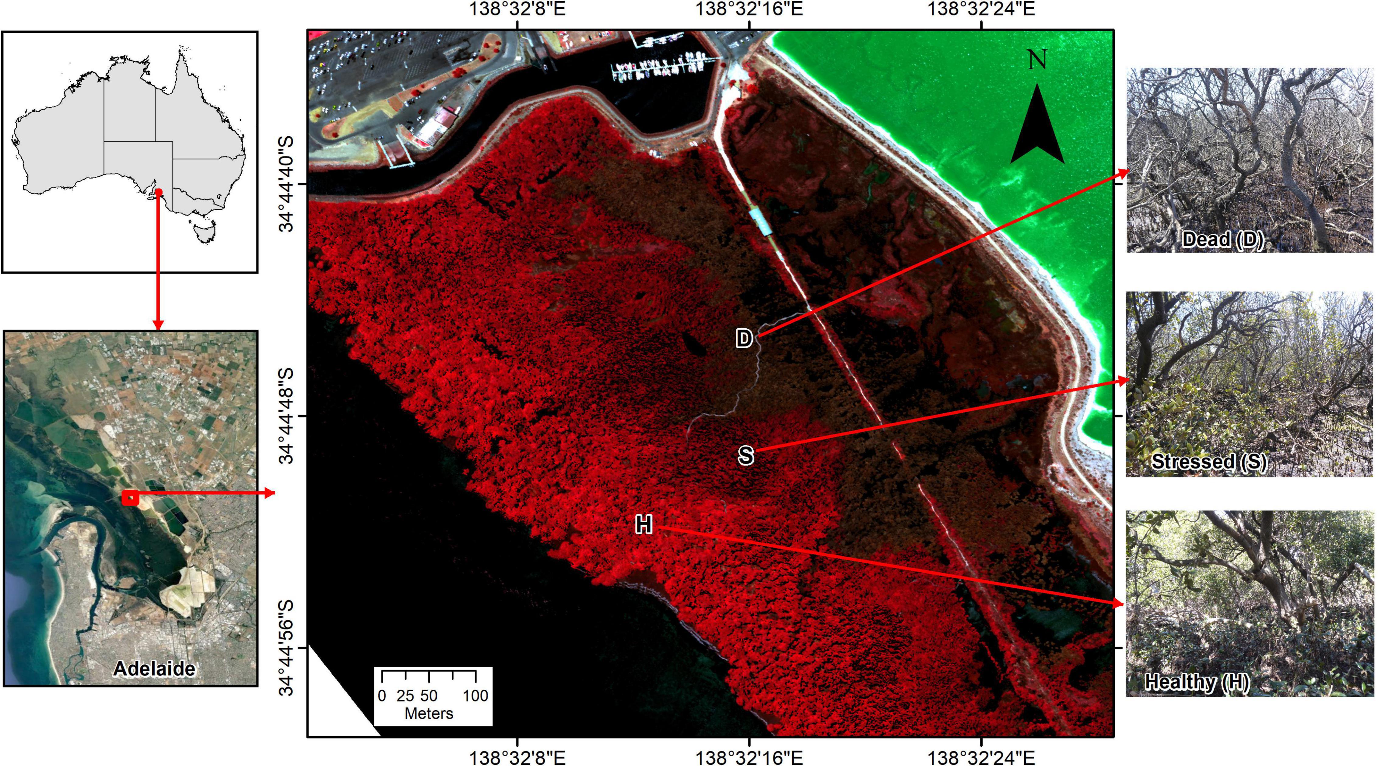
Figure 1. Location of studied temperate mangrove forest near St Kilda, Gulf St. Vincent, South Australia, with sampling locations across zones from “healthy” (H, near seaward edge) to “dead” mangrove (D, near former sea wall), with a “stressed” (S) zone in between. The underlying Color-Infrared (CIR) image from January 2021 shows healthy vegetation in bright red, dead foliage in brown and the hypersaline salt pond inland from the mangrove and saltmarsh in bright green.

The mangrove forest is monospecific composed of Avicennia marina. While the dieback was recorded in a wider area of mangrove in Barker Inlet, our investigations focused on a location near the township of St Kilda, where the dieback was extensive (Department for Environment and Water, 2021a) and where a boardwalk provided easy access to the mangroves. The mangrove forest is narrow at this location, with a distance of about 400 m from the landward to the seaward edge. Remains of a former sea wall constitute a landward barrier, with saltmarsh extending further inland in the upper intertidal. The seaward levee banks of Dry Creek salt field are located ∼100 m inland from the former sea wall. Commercial salt production ceased in 2013 and the salt field has been in a holding pattern since. The ponds behind the mangroves in Barker Inlet are close to the former crystallizer ponds where salt was harvested and a zone of active gypsum mineral (CaSO₄.2H₂O) precipitation with thick crystal deposits. Halite (NaCl) also precipitated once the ponds drained and salinities rose. In December 2019, the salt field operator began refilling the ponds with hypersaline water from adjacent northern parts of the salt field (Department for Energy and Mining, 2022a). Upon refill back to operational levels, water levels were elevated (approximately 1 m) above adjacent coastal ecosystems.

The mangrove dieback became apparent along the boardwalk by September 2020, and targeted investigations commenced shortly after (Supplementary Figure 1). In-depth investigations occurred in July and October 2021 and data from both survey dates were combined for the assessment. For CO₂-flux, additional measurements were carried out in August and November 2021. All sampling and field measurements occurred at low tide between 9 am and 4 pm. Data from before the dieback were available from our earlier investigations in the area, which were carried out for different objectives. See Supplementary Table 1 for an overview of the sampling design.

Airborne Assessment of Mangrove Health

From March 2018 through to March 2021, airborne remote sensing data of the affected area were collected from Airborne Research Australia’s “Eco-Dimona” special mission aircraft (Supplementary Table 2). Ultra-high resolution RGB imagery from October 2020 captured an early stage of the dieback (Supplementary Figure 2). To separate the mangroves from other vegetation, a simple 1.2 m height thresholding of a canopy height model derived from the January 2021 LIDAR showed a very good discrimination (Supplementary Figure 2).

Hyperspectral data were available from 2018, before the dieback occurred, and from two occasions (January and March 2021) after the dieback started. All hyperspectral image sets were captured with the same instrument, a modified Specim Eagle 2 VNIR linescanner, and with the same spectral settings, configured for 62 bands spanning 400–1000 nm. After radiometric correction, atmospheric correction to surface reflectances, georeferencing and mosaicking to a coherent hyperspectral GIS layer, a supervised Mahalanobis distance classifier was used to classify the mask-selected mangrove areas as “healthy,” “stressed,” or “dead.” This Mahalanobis distance classifier was initialized using training areas delineated manually from RGB, color-infrared and NDVI (Normalized Difference Vegetation Index) images to select clearly dead areas, areas of apparent health far from the dieback zone showing high NDVI, and areas adjacent to the dieback zone with slightly reduced NDVI. Non-mangrove classes – exposed water, crystallized salt, bare soil, and jarosite – were also included in this analysis to provide clearer separation but these were subsequently eliminated by the height-selected mangrove masking described above to derive the classification layer shown in Figure 2. The “healthy,” “stressed,” and “dead” mangrove zones were used for additional land-based and proximal measurements as described below.

FIGURE 2

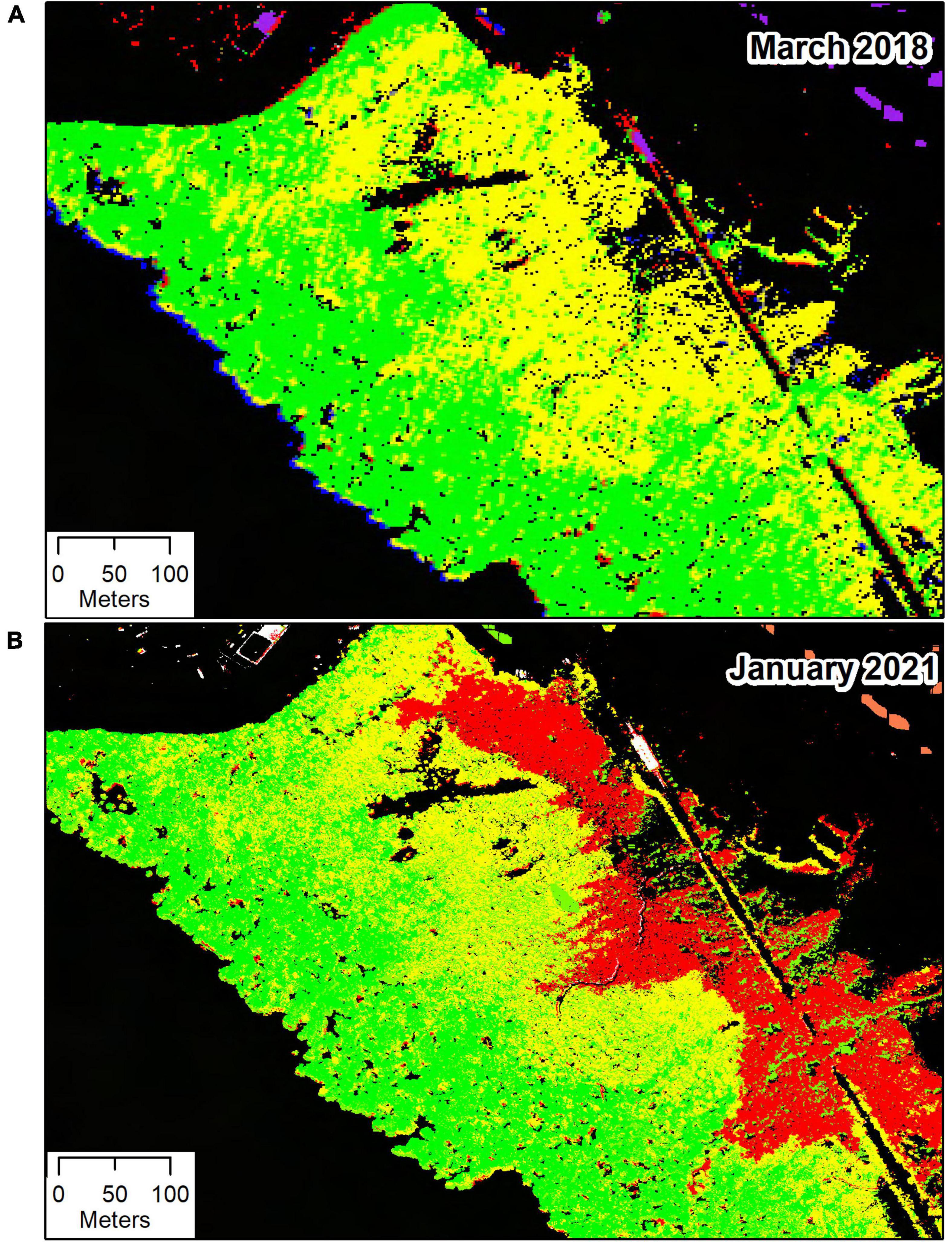
Figure 2. Hyperspectral images from the temperate mangrove forest (saltmarsh and other vegetation was masked out) near St Kilda, South Australia, from March 2018 (A) and January 2021 (B). Mangroves were classified as “healthy” (green), “stressed” (yellow), and “dead” (red).

Salinity, Soil Properties, Carbon Stock, and CO₂ Flux

Porewater samples were collected using suction lysimeters. A suction lysimeter includes a ceramic cup connecting to a tube (1 m long, about 5 cm diameter) with an open top sealed by a rubber stopper. Before installation, a negative pressure (−80 kPa or lower) is established in the lysimeter using a suction pump attached with a pressure gauge. The suction lysimeters were installed in soil with the ceramic cups at a depth of 15 cm below the soil surface, as A. marina have a shallow root system (Hu et al., 2021). Water samples collected in over 2 h and were immediately transferred to a sample container, where the salinity was measured using a calibrated electrical conductivity meter (a YSI multimeter instrument in 2018, a WTW pH/Conductivity meter in 2020 and 2021). Porewater samples were taken at three sites along the boardwalk in October 2018, and at nine sites in October 2020, which corresponded to the later impact zone classifications but with an uneven sample size per impact zone. Porewater salinity was sampled at seven sites along the “dead” and “stressed” zone in July 2021.

For comparability with other studies, electrical conductivity (EC, in mS/cm) was converted to salinities using equation (1)

Salinity = - 7 E - 06 * {EC}^{3} + 0.003 * {EC}^{2} + 0.5865 * EC (1)

based on relationships established using gravimetric salinity measurements following strict quality control and assurance procedures in a National Association of Testing Authorities (NATA) accredited laboratory for a local estuarine-hypersaline lagoon (Mosley et al., 2020).

Soil samples were collected at each of the three plots in the three zones. Five 0–50 cm depth soil profiles were collected for each plot using a gouge auger (50 mm × 1 m, Dormer Pty Ltd, Murwillumbah, South Australia). Each core was divided into horizons of 0–10, 10–20, 20–30, and 30–50 cm depth and composite samples taken for each depth interval. A sub-sample of the composite was collected in a 70 mL vial and frozen for laboratory analysis. Samples were oven dried (40°C), finely ground and sieved to <0.5 mm. pH and EC were measured on a 1:5 soil:water extract (Slavich and Petterson, 1993). SOC on the dried sample was analyzed via dry combustion and infrared detection (LECO Trumac instrument). SOC results are reported on an oven dried basis at 105°C following separate measurement of moisture content via mass loss at this temperature. Bulk density measurements were obtained by pushing metal rings of known volume into the soil, using a soft mallet on another ring placed on top of the sample ring, and determining oven dry (at 105°C) soil weight in the ring volume. Soil carbon stocks in mass per unit area (t C ha–¹) over 50 cm depth were calculated using equation (2), following Howard et al. (2014) and the VM033 method (VCS, 2015):

SOCstock = \sum_{i = 1}^{N d e p t h} (C_{SOC %} x BD x Thickness) (2)

N_depth is the number of soil horizons, based on subdivisions of soil cores; C_SOC% is the SOC of each soil horizon sample (as determined in laboratory, %C); BD is the bulk density (g cm^–3), and thickness (cm) of the soil horizon which was measured. Sulfate and chloride concentrations were determined in a 1:1 water extract, and analyzed in a NATA accredited laboratory following strict quality control and assurance procedures by ICP-OES for the sulfur content and converted to sulfate by calculation, and by ICP-MS for chloride.

Soil redox potential (Eh) was measured by pressing a fiberglass rod probe (Paleoterra, Oijen, Netherlands) into the soil. Multiple platinum electrodes were embedded along the rod at 1, 5, 10, 25, and 50 cm depths below ground level. A separate Ag/AgCl reference electrode filled with saturated KCl gel was installed in close proximity to the redox sensor. The redox and reference electrode were connected to a datalogger (Campbell CR1000) and the redox potential (Eh) tested using Zobell’s standard solution. For each site measurement, Eh was logged for at least 30 min, at which point readings had stabilized such that a measured value was recorded. Field Eh readings were corrected to that which would be obtained using a standard hydrogen electrode, by adding the known potential of the reference electrode at ambient temperature.

Measurements for CO₂ flux between mangrove soil and atmosphere were carried out with an automated soil gas flux system LI-8100A (LI-COR Biosciences; Lincoln, NE, United States) using the 20 cm soil collars and survey chamber. The soil collars were inserted into the soil to between 5.5 and 8 cm depth to assure solid foundation and minimize lateral diffusion of CO₂ in the soil column. For each zone (“healthy,” “stressed,” and “dead”) three sampling locations were selected, trying to minimize the number of aerial roots (pneumatophores) inside the sampling area. The 20 cm soil collars and survey chamber were set to take three measurements at each location with an observation length of 150 s, a 30 s pre-purge (to allow the chamber air to return to ambient conditions) and a 30 s post-purge (to clear the gas sampling lines) between measurements. The CO₂ efflux for each zone was calculated based on the values for the three sampling locations for each zone.

Forest Structure and Biomass

Aboveground tree biomass was assessed in three plots positioned within each of the three zones. Due to variation in tree densities across the zones, plot sizes of 5 × 5 m, 8 × 8 m, and 10 × 10 m were sampled for the “dead,” “stressed,” and “healthy” zones, respectively. Tree height and stem circumference at 30 cm above the ground level were measured for the trees rooted within the plots. Biomass was calculated using an allometric equation based on tree height and stem diameter at 30 cm (D₃₀) developed in this local area (Jones et al., 2020). The allometric equation (3) takes the form;

Biomass (kg) = (exp (- 5.9376 + 0.6328 \times \log (Height) + 2.2310 \times log (D_{30}))) \times CF (3)

The correction factor (CF) for back-transformation of logarithmic prediction was 1.05855 and calculated using the method described by Sprugel (1983). For multi-stemmed trees, D₃₀ was calculated using the square root of the sum of the squared D₃₀ values for all stems in each tree (Jones et al., 2020). Biomass estimates for individual trees were summed to the plot level. The dead trees in the dieback zone were in decay status 1 (trees remain standing, retain small branches and twigs, but shed leaves) for which leaves should be subtracted from the biomass estimate (Howard et al., 2014). Based on data from Jones et al. (2020), the relative contribution of leaves to the biomass of A. marina in South Australia was 16.4% ± 1.6. We used this local value to account for loss of leaf biomass in the dead trees. A locally derived carbon content value of 44.3% for A. marina (Jones et al., 2020) was used to convert biomass to above-ground carbon stock (t C ha^–1).

Normalized Difference Vegetation Index, Photosynthetic Traits and Leaf Nutrient Measurements

All plant measurements of A. marina were taken in the “healthy” and “stressed” zone as trees in the “dead” zone were defoliated. The measurements for NDVI were taken on four plants from each of the two zones and four second youngest leaves on each plant. For all other photosynthetic traits and leaf measurements, seven plants were randomly selected from each of the “healthy” and “stressed” zone and four different second youngest leaves used for measurements on each plant or collected for nutrient analyses in the laboratory.

Normalized Difference Vegetation Index was measured using a hand-held meter (PlantPen NDVI 300, Photon System Instruments, Drásov, Czech Republic). Gas exchange was measured using a portable photosynthesis system from a time of 11:00 to 13:00 h. The light source was the Multiphase Flash™ Fluorometer (6800-01A, LI-COR, Nebraska, United States) and light intensity was set at 800 μmol m^–2s^–1 (90% red, 10% blue) with an aperture of 6 cm². All photosynthetic measurements were taken when photosynthetic rate and stomatal conductance were stable at a constant airflow rate of 500 μmol s^–1. The CO₂ concentration supplied was 400 μmol mol^–1 and the temperature (Tair) was 18°C. The humidity of the chamber was controlled by setting leaf vapor pressure deficit (VDP_leaf) = 1.5.

The chlorophyll fluorescence parameter (Fv/Fm) was measured using a portable photosynthesis system (LI-6800, LI-COR, Nebraska, United States) and a hand-held meter (FluorPen FP 100, Photon System Instruments, Drásov, Czech Republic). Leaves were adapted to dark by wrapping with aluminum foils for 1 h before the measurement. For the LI-6800 system, the measurement was taken with the actinic light off and dark mode rate set to 50 Hz. The flash was rectangular with the red target 8000 μmol m^–2s^–1, duration 1000 ms, output rate of 100 Hz and margin of 5 points. In this process, minimal fluorescence (F_o) was measured before flash and maximal fluorescence (F_m) was measured when flash. The variable fluorescence and maximum quantum yield of PSII were calculated as described by Maxwell and Johnson (2000). For the hand-held meter, F_pulse and f_pulse were set at 50 and 30% respectively.

For leaf nutrient analyses, individual leaves were ground with a Retsch ZM200 mill (Retsch, Haan, Germany). For inductively coupled plasma mass spectrometry (ICP-MS) analysis, ∼0.3 g of each ground sample, which had been oven dried at 80°C for 4 h to remove remaining moisture, was acid-digested in a closed tube as described in Wheal et al. (2011). Elemental concentrations of samples were measured using ICP-MS (8900; Agilent, Santa Clara, CA, United States) at Flinders University. The reference material used for the ICP-MS analysis was “WEPAL IPE-192” string bean pods.

Carbon, hydrogen and nitrogen were determined by combustion, using the Dumas method. Approximately 0.01 g finely ground leaf tissue was used for analysis using a vario EL cube (Elementar Analysensysteme GmbH, Langenselbold, Germany) (Jung et al., 2003). A certified reference material (WEPAL IPE-684 wheat grain) was used to confirm the accuracy of analysis.

Data Analysis

Soil and mangrove properties were tested for differences between the seaward side of the mangrove forest (the “healthy” zone) over the “stressed” zone to the landward side (the “dead” zone). Soil characteristics were also tested over sediment depths. For porewater salinity and CO₂-flux from soil, time (survey date or month) were additional factors. Data exploration was applied following the protocols described by Zuur et al. (2010). Normality (Shapiro–Wilk test; Q-Q plot) and homogeneity (Levene’s tests; conditional boxplot) were not met for most soil variables and salinity (Zuur et al., 2010), thus PERMutational ANalysis Of VAriance (PERMANOVA) were performed. Differences in porewater salinity were tested for October 2020 and July 2021, where several replicate samples per “stressed” and “healthy” zone were available, using a two-way PERMANOVA. In further two-way PERMANOVAs, soil salinity, pH, organic carbon, redox potential, sulfate and chloride were tested each with zone and depth as factor, and CO₂-flux for differences between zones and months. To test for differences in forest structure and carbon stocks in biomass and soil, one-way ANOVA were carried out with zone as factor. PERMANOVA were performed in PRIMER v7 with PERMANOVA add-on (Anderson et al., 2008), and tests for normality, homogeneity of variance and ANOVA in Origin Pro (v2020b). For photosynthesis traits and leaf nutrients, statistical analysis was performed using R software v.4.0.3 (R Development Core Team, 2018). The mean comparison between two locations was analyzed using Student’s t-test. The test was performed on the mean value of each plant.

Results

Airborne Assessment of Mangrove Forest

The classified hyperspectral datasets show the temporal progression, with no mangrove dieback apparent in 2018, but evident adjacent to the salt pond bund wall in the January 2021 imagery (Figure 2). Color-infrared imagery derived from the hyperspectral data collected on the 16th of January and the 18th of March 2021 shows little or no change in the extent of dieback between these dates (Supplementary Figure 3). The spatial distribution of the classified stress zones was not related with the topography at the site, as a high quality, high resolution digital terrain model derived from LIDAR measurements in both January and March of 2021 showed undifferentiated ground with a very gentle slope (Supplementary Figure 4).

The hyperspectral classification images from both years show presence of possibly stressed mangroves, with a similar spatial distribution pattern in 2018 as in 2021. This may indicate a chronic stress unrelated to the recent dieback.

Salinity

Porewater salinity in the mangrove root zone increased from the seaward to the landward sections of the mangrove forest, with salinity ranging from 35 to 43 in the “healthy” zone but exceeding seawater salinities on most sampling occasions in the “stressed” and “dead” zone (Figure 3A). Salinity records in the “stressed” zone ranged from 37 to 66. In the landward sections, salinities were ≤50 before the dieback. In October 2020, shortly after the mangrove dieback became evident, porewater salinity in this “dead” zone was extremely hypersaline (98.5 ± 5.5 mean ± standard error, range 84 – 109) (Figure 3A and Supplementary Table 3). This increase did not persist by July 2021, when porewater salinities were similar to values in 2018. Soil salinity (1:5 soil:water extract) was significantly higher in the “dead” zone in mid-2021, and hypersaline (>2 × seawater salinity) at greater depths (Figure 3B and Supplementary Table 3).

FIGURE 3

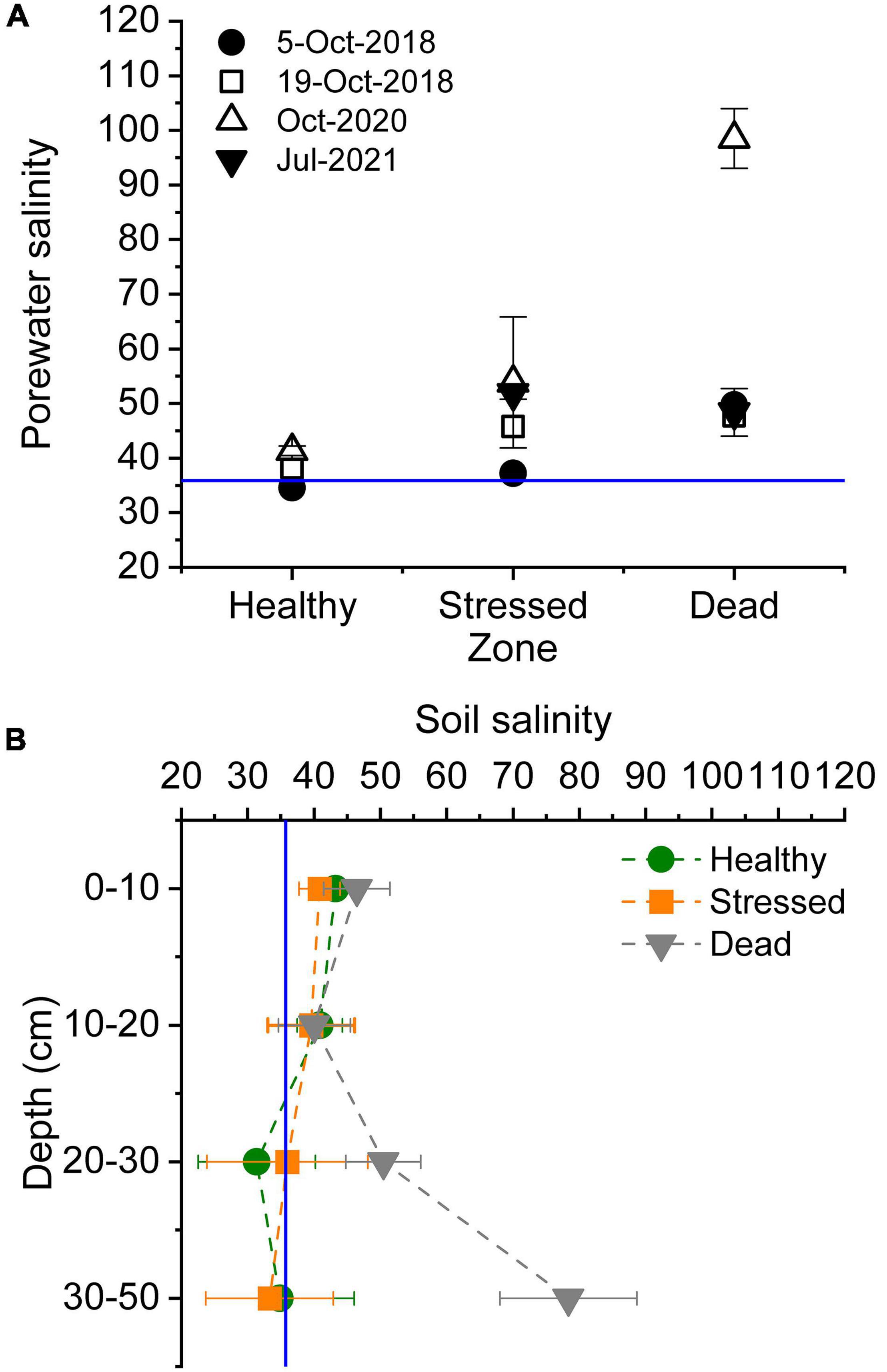
Figure 3. Salinities throughout the mangrove zones at St Kilda, South Australia, in (A) porewater in the shallow root zone of mangrove measured on several occasions before and after the dieback commenced (October 2020), and (B) in soil (1:5 soil water extract) over several depth measured in mid-2021. The blue lines indicate mean seawater salinity.

Soil Characteristics and CO₂ Flux

The biogeochemical properties of the mangrove soil varied across the three zones, with largest differences between the “healthy” and “dead” zone (Figure 4 and Supplementary Table 4). The redox potential was significantly lower at all depths in the “dead” zone, and less oxidized at shallower sediment depths than in the “stressed” and “healthy” zones. Total organic carbon decreased significantly with depths but did not vary between zones. pH appeared slightly more alkaline at greater depths in the “stressed” zone, but was not significantly higher. Both sulfate and chloride concentrations were low in surface sediments but increased with depth (>30 cm below ground level) in the “dead” zone, which was opposite to the pattern with depth seen in the “stressed” zone. There was less variation with depths for both sulfate and chloride in the “healthy” zone.

FIGURE 4

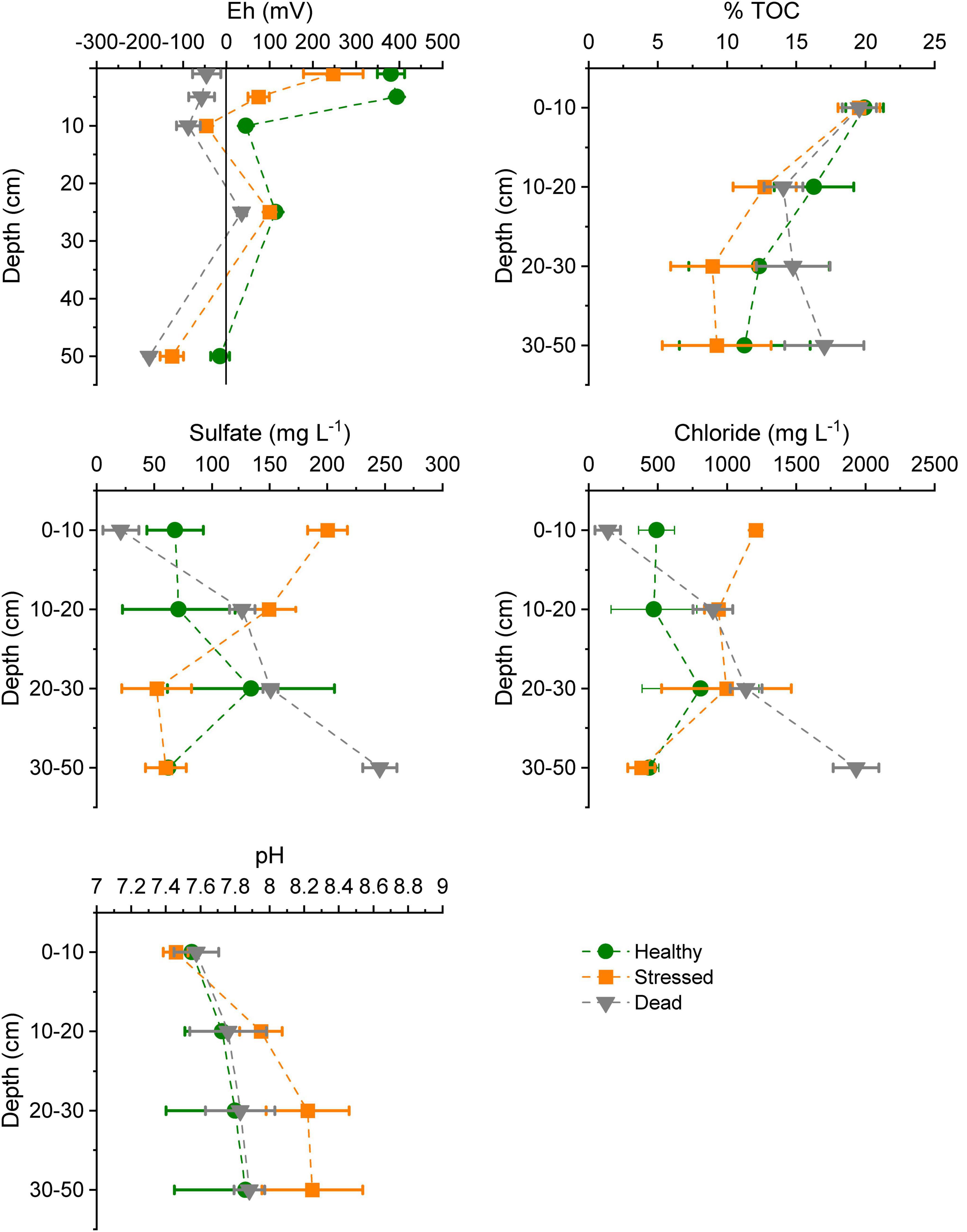
Figure 4. Soil characteristics at the three mangrove zones at St Kilda, South Australia, measured in mid-2021, showing mean ± standard error based on samples from two to three plots per zone. TOC, total organic carbon.

The CO₂ flux was highly variable, and no significant differences were detected between the zones and months of measurements (Figure 5 and Supplementary Table 4). Across all times and zones, the average CO₂ flux was 0.77 μmol m^–2 s^–2 (range 0.47–1.44 lowest to highest average value).

FIGURE 5

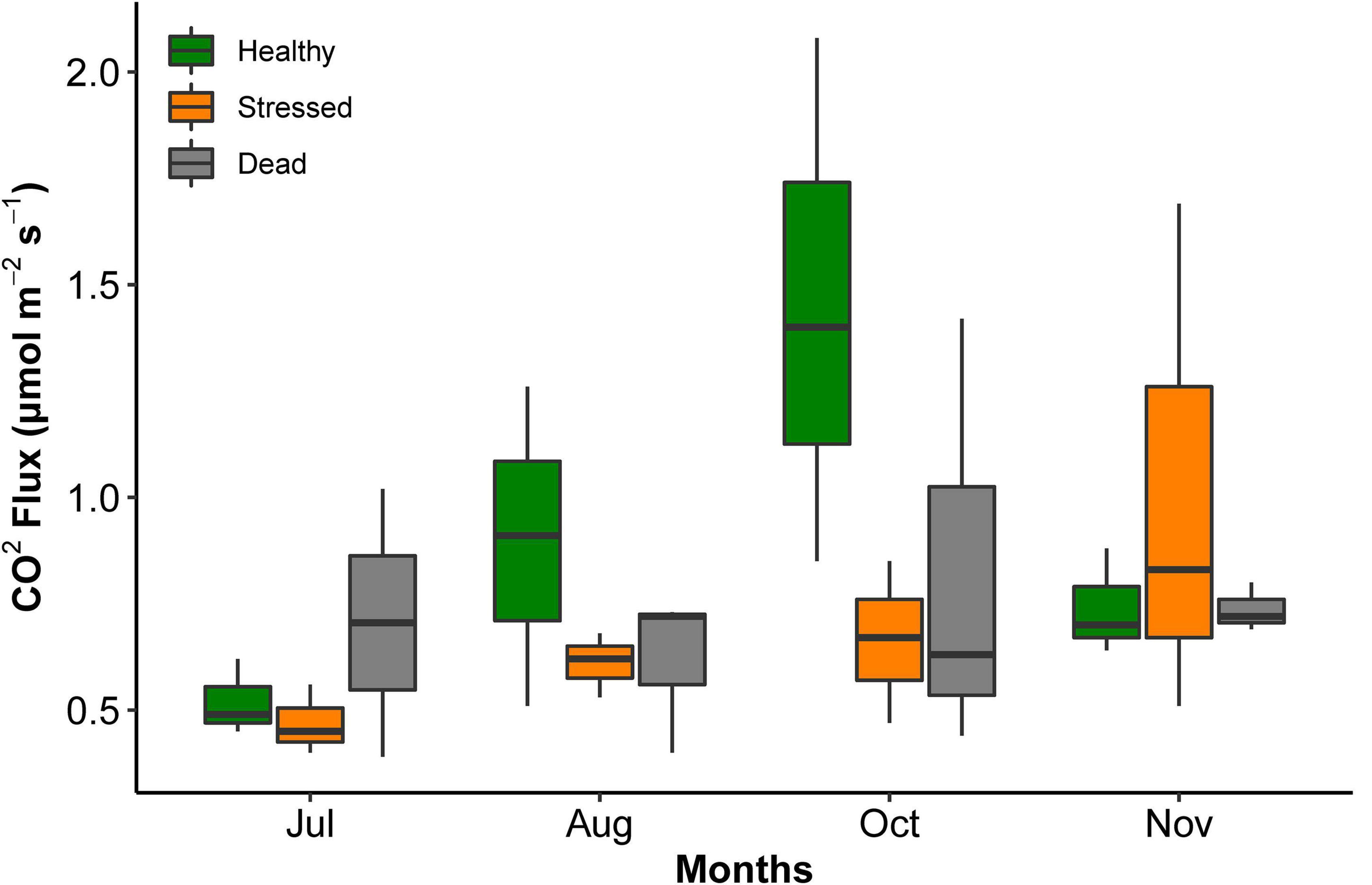
Figure 5. CO₂ efflux from sediment at the three mangrove zones at St Kilda, South Australia, measured over several months in 2021. All measurements were taken at low tide. There were no significant differences between the zones and months.

Mangrove Forest Structure and Carbon Stock in Biomass and Soil

Forest structure (height and tree density) changed significantly across the zones reflecting the position of the zones across the seaward-landward gradient (Figure 6 and Supplementary Table 5). Tree height (mean ± standard error) was 2.68 ± 0.28, 3.23 ± 0.34, and 4.77 ± 0.65 m in the “dead,” “stressed,” and “healthy” zones, respectively. The increase in forest height was associated with a decrease in tree density per plot (Figure 6). Biomass and the aboveground carbon stock were similar between the “healthy” and “stressed” zones (approx. 48 t C ha^–1 on average) and tended to be lower (31.45 ± 2.93 t C ha^–1) in the “dead” zone where trees were in decay status 1, but no significant difference was detected across the three zones (Supplementary Table 5). The soil carbon stock in the “healthy” zone was 101.72 ± 15.97 t C ha^–1, and soil carbon was not significantly different across the zones. In the “dead” zone, the carbon stock from aboveground biomass and soil combined amounted to 157.78 ± 24.4 t C ha^–1.

FIGURE 6

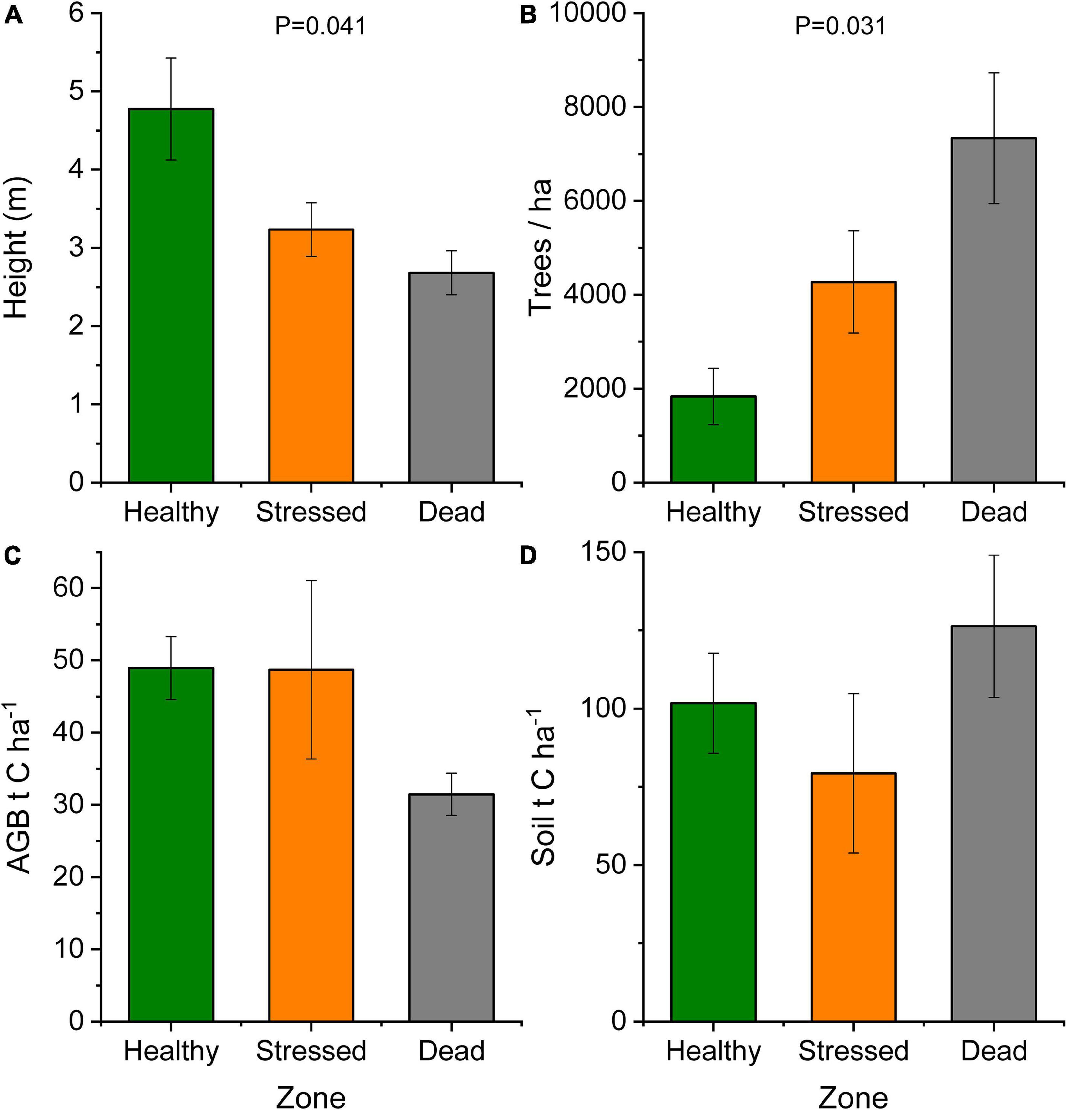
Figure 6. Mangrove forest characteristics at St Kilda, South Australia, showing mean ± standard error for (A) tree height and (B) tree density across mangrove zones. The carbon stock is shown for (C) above-ground biomass (AGB) and (D) soil to 50 cm depth across the mangrove zones. Trees in the “dead” zone constitute necromass and were in decay status 1.

Photosynthetic Traits and Leaf Nutrients

The leaf color of healthy plants was greener than the leaf color of stressed plants which also showed a yellowing (chlorosis) of leaf tissue (Supplementary Figure 5). Particularly, the “healthy” plants (0.79 ± 0.001) had significantly (P < 0.001) higher leaf NDVI (a measure of leaf “greenness”) than the “stressed” plants (0.65 ± 0.018) (Figure 7). Photosynthetic parameters of the “stressed” plants were significantly affected in comparison with the “healthy” plants. For example, photosynthetic rate of the “healthy” plants was 8.5 ± 1.4 μmol CO₂ m^–2s^–1, 63.5% higher (P < 0.01) than that of the “stressed” plants (Figure 8). The “healthy” plants (329.5 ± 41.6 μmol CO₂ mol^–1) also had 25.1% higher (P < 0.05) intercellular CO₂ concentration than the “stressed” plants (Figure 8). The “healthy” plants had 3.3-fold higher (P < 0.05) stomatal conductance (0.37 ± 0.26 mol H₂O m^–2s^–1) and 2.8-fold higher (P < 0.05) transpiration rate (0.004 ± 0.0015 mol H₂O m^–2s^–1) than the “stressed” plants (Figure 8). The maximal potential quantum efficiency of photosystem II (F_v/F_m) was significantly (P < 0.01) lower in the “stressed” plants (0.65 ± 0.072) than the “healthy” plants (0.77 ± 0.014) (Figure 9).

FIGURE 7

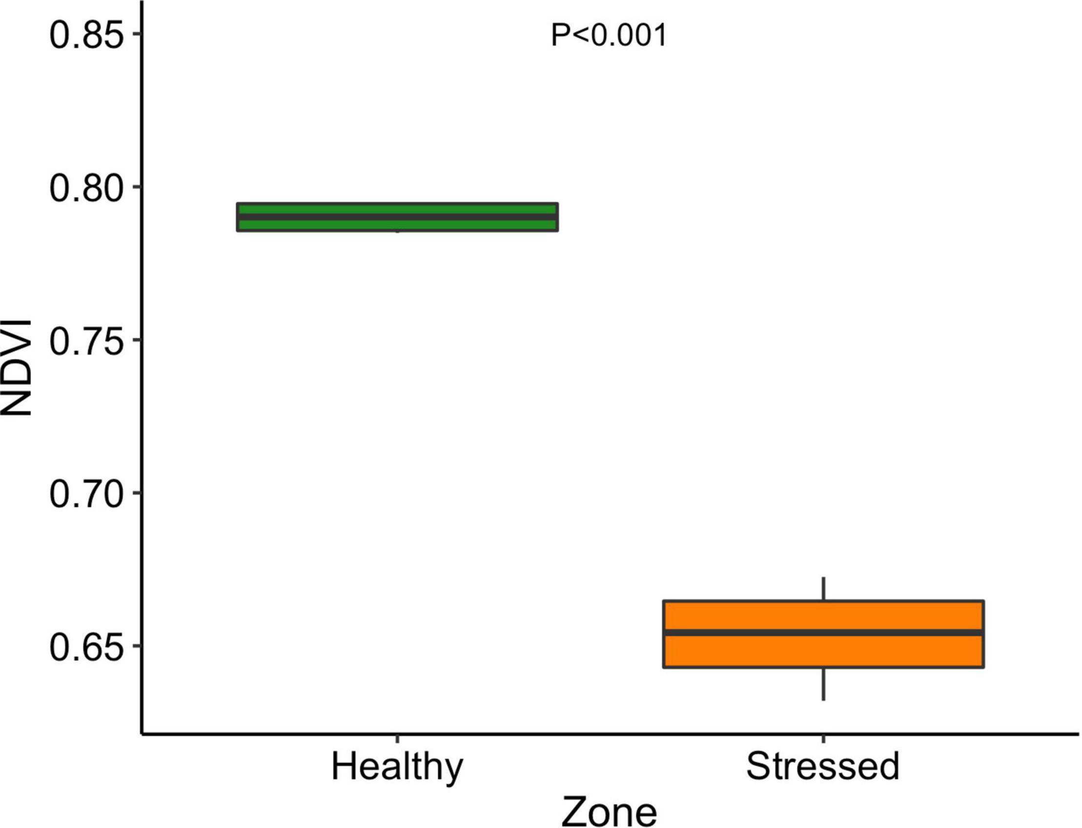
Figure 7. Normalized Difference Vegetation Index of “stressed” and “healthy” Avicennia marina at the St Kilda mangrove forest, South Australia. The measurements were taken on the second youngest leaves. Four leaves were measured from each plant and four plants were measured from each zone.

FIGURE 8

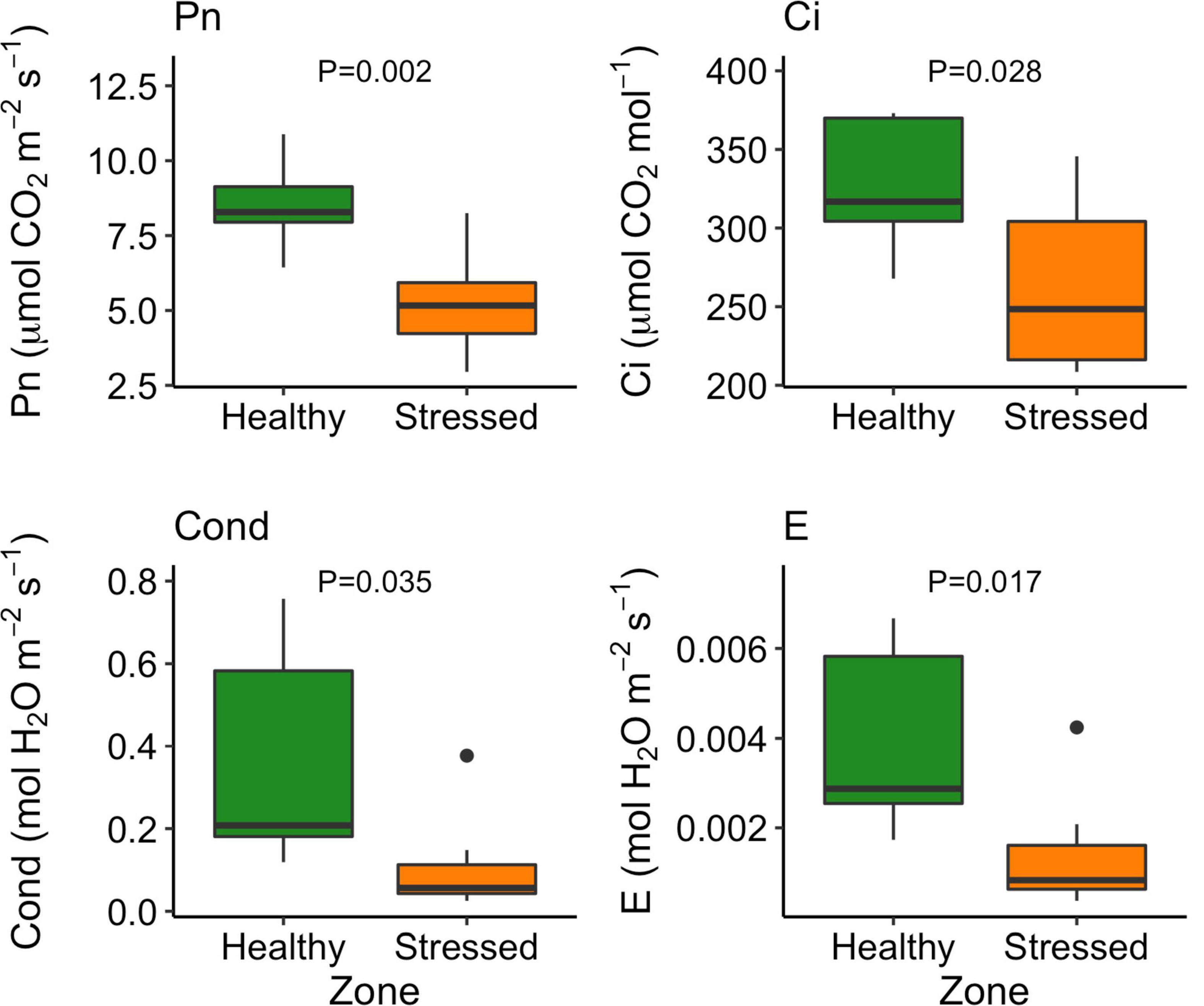
Figure 8. Variation in photosynthetic rate (Pn), intracellular CO₂ concentration (Ci), stomatal conductance (Cond), and transpiration rate (E) between “stressed” and “healthy” Avicennia marina at the St Kilda mangrove forest, South Australia. The measurements were taken on the second youngest leaves. Four leaves were measured from each of seven plants per zone.

FIGURE 9

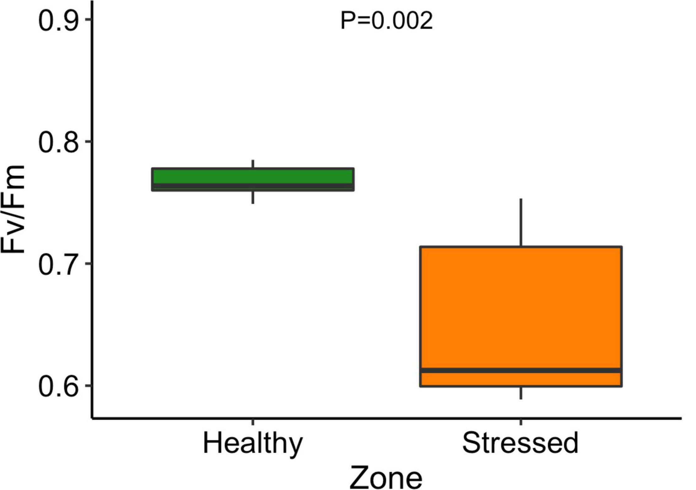
Figure 9. Maximal chlorophyll fluorescence (Fv/Fm) of “stressed” and “healthy” Avicennia marina at the St Kilda mangrove forest, South Australia. The measurements were taken on the second youngest leaves. Four leaves were measured from each of seven plants per zone.

Eighteen nutrients were analyzed in A. marina leaves collected from the “stressed” and “healthy” zones (Figure 10). The “healthy” plants had significantly higher calcium, sodium and phosphorus concentrations than the “stressed” plants (Figure 10). The concentrations of calcium, sodium and phosphorus in the “healthy” leaf were 5.12 ± 0.67 g kg^–1, 34.66 ± 4.94 g kg^–1, and 2.99 ± 0.83 g kg^–1, respectively, while these concentrations in the stressed leaf were 2.26 ± 0.27 g kg^–1, 24.35 ± 4.98 g kg^–1, and 1.83 ± 0.44 g kg^–1, respectively (Figure 10). Leaf molybdenum concentration was also higher in the “healthy” leaf (0.19 ± 0.03 mg kg^–1) than in the “stressed” leaf (0.09 ± 0.02 mg kg^–1). In contrast, arsenic, sulfur and zinc concentrations were significantly higher the “stressed” leaf than in the “healthy” leaf. The sulfur concentration of the “stressed” leaf (16.06 ± 6.61 g kg^–1) were about four times higher than in the “healthy” leaf. The leaf arsenic and zinc concentration in the “stressed” leaf were 1.23 ± 0.57 and 45.5 ± 12.9 mg kg^–1, respectively, while these concentration in the “healthy” leaf were 0.62 ± 0.17 and 22.5 ± 10.5 mg kg^–1, respectively (Figure 10).

FIGURE 10

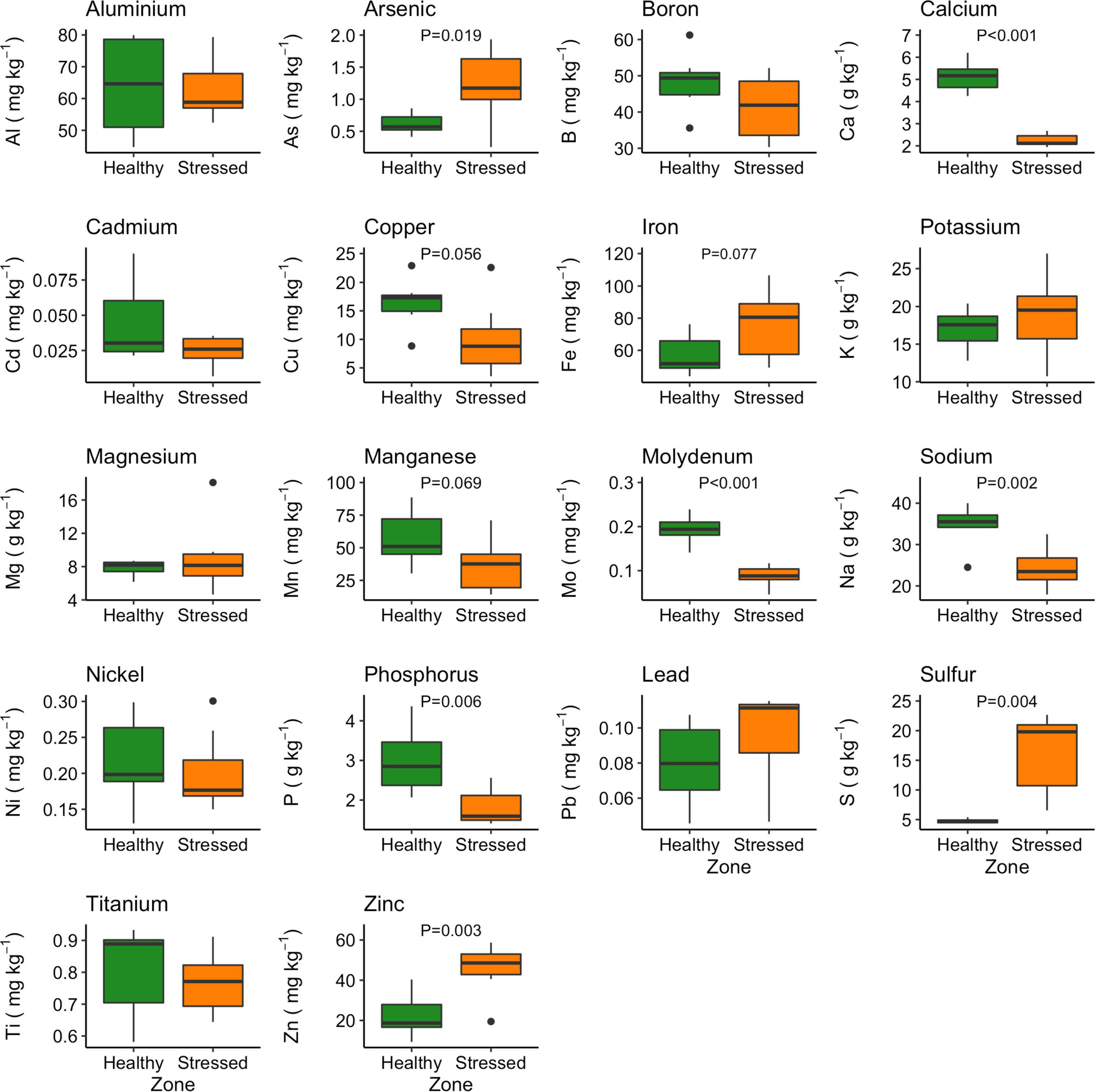
Figure 10. Variation in leaf nutrients between “stressed” and “healthy” Avicennia marina at the St Kilda mangrove forest, South Australia. The analyses were done on the second youngest leaves. Four leaves were sampled from each of seven plants per zone. P-values are only shown for significant differences.

There were no significant differences in leaf hydrogen between leaves from the “stressed” and “healthy” zone. However, the “stressed” leaf had significantly (P < 0.05) higher carbon content but significantly (P < 0.01) lower nitrogen content than the “healthy” leaf. The carbon and nitrogen contents in the “stressed” leaf were 44.9 ± 0.6% and 1.68 ± 0.20%, while these contents in the “healthy” leaf were 43.9 ± 0.2% and 2.37 ± 0.24% (Figure 11).

FIGURE 11

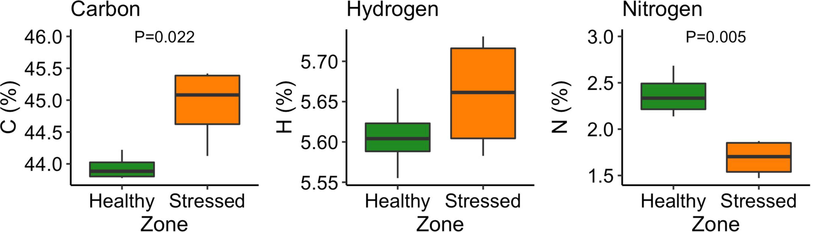
Figure 11. Carbon, hydrogen and nitrogen content of Avicennia marina leaves under “stressed” and “healthy” conditions at the St Kilda mangrove forest, South Australia. The analyses were done on the second youngest leaves. Four leaves were sampled from each of seven plants per zone. P-values are only shown for significant differences.

Discussion

Our study reports on one of the most severe (porewater salinity > 100) known cases of hypersalinity-driven dieback in mangrove ecosystems. Effects of extreme hypersalinity on the temperate mangrove studied included dieback of parts of the mangrove forest and degradation of mangrove health in areas adjacent to the dieback. Our multidisciplinary approach gave evidence of differences in mangrove health from remote sensing, which was corroborated by field measurements in zones classified as “healthy,” “stressed,” or “dead.” All photosynthetic traits measured were lower in leaves from the “stressed” than “healthy” zone, and leaf nutrient analyses indicated further impairment of plant health in “stressed” leaves. While the findings indicate impact of the extreme salinity on mangrove trees beyond the immediate dieback zone, carbon stocks of mangrove biomass and SOC were not different between zones in this first year after the event. Effects on the carbon cycle following the dieback thus merit further investigations.

Differences in Soil Properties and Salinity

Our analyses revealed differences in the sedimentary conditions between the zones, which were most pronounced between the “healthy” and “dead” zones. Sediment conditions in the “stressed” zone were mostly intermediate between the two other zones, but were enriched with sulfate and chloride at shallower depths. Sediments in the “dead” zones were hypersaline and contained higher concentrations of sulfate and chloride, particularly in deeper horizons. While we did not make measurements within the salt field, in general sulfate and chloride are in high concentrations in the hypersaline brine and are key elements of gypsum and halite minerals respectively (Jeschke et al., 2001). The higher concentrations with depth in the soil profile are consistent with upward seepage arising from an elevated head of hypersaline groundwater. The mangrove ecosystem is flushed with seawater regularly via tidal action which explains less difference between near surface salinities in the different zones. Flushing is stronger at the seaward side of the forest where it would buffer mangrove from the development of hypersaline conditions in porewater (Lovelock et al., 2009). At the landward side of the mangrove forest, which was adjacent to the salt pond, less frequent tidal inundation can exacerbate hypersaline conditions.

The redox profiles showed reducing conditions at all sediment depths in the ‘dead’ zone. Avicennia marina can oxidise sediments around its roots and in the rhizosphere (Alongi et al., 2000). The more anaerobic surface sediment conditions in the “dead” zone are likely due to lack of root-based aeration of the soil, following the mangrove death.

Soil organic carbon showed no clear pattern across the zones, as a large proportion of the carbon is likely to be stable or buried in the wet soil profile, over the relatively short timeframes (<1 year) from the dieback to when we sampled. However, other studies have found very rapid carbon loss in soils in the first few years after mangrove mortality, before a more gradual depletion over decades (Sippo et al., 2020). The loss of soil carbon after mangrove death or removal for land use changes arises from loss of mangrove root volume, increasing compaction and bulk density (Sasmito et al., 2019). While the root decomposition rate is high for A. marina (0.20% d^–1 in temperate latitudes), decay rates are slower under high porewater salinities (Ouyang et al., 2017), which could contribute to the lack of difference in SOC between the zones in our study. With ongoing root decomposition and as new organic matter is not being created by plant production in the “dead” zone, there are likely to be longer term effects of the dieback on soil carbon stocks.

Porewater salinity recorded during the mangrove dieback event (98.5 on average) was nearly 3x higher than seawater salinity, and a year after the dieback, soil salinity (1:5 soil:water extract) was 2x seawater salinity at depth. This is >16 times seawater salinity when converted to a saturated paste extract using the relationship for a clay-loam of Slavich and Petterson (1993, see Table 1 therein). Overall our salinity measurements align with groundwater measurements by the Department for Energy and Mining (2022b) which recorded salinity in the saltmarsh between the salt pond and mangrove of approximately 140 to >200 in early 2021 before a decrease in the following months, but groundwater salinities remained > 100. Other cases of mangrove dieback were recorded at porewater salinities from >68.5 (Lovelock et al., 2017a) to >93 (Senger et al., 2021). The hypersaline brine seepage at the St Kilda mangrove in South Australia was thus indeed an extreme salinity event. Mangrove mostly access porewater, but can also access groundwater (Lovelock et al., 2017b), yet the hypersaline groundwater in impacted areas at St Kilda would have limited the use of this as an alternative water source.

Differences in Mangrove Plant Physiology

As a measure of mangrove tree health, photosynthetic parameters and leaf tissue nutrient composition were measured. The NDVI can give an indication of vegetation vigor and the lower NDVI in “stressed” compared to “healthy” mangrove was similar to reductions in NDVI seen during hypersalinity induced mangrove dieback (Lovelock et al., 2017a), and dieback due to ENSO (El Niño-Southern Oscillation) related inundation and sea level changes (Asbridge et al., 2019). NDVI can be a sensitive indicator for change in mangrove ecosystems, especially those subjected to cumulative pressures (Maina et al., 2021). Linked to the NDVI are leaf N levels which were significantly reduced in stressed leaves. The significant reduction of P in stressed plant leaf tissue could be a major contributor to the poor photosynthetic performance that eventually led to leaf drop. P is an essential component of ATP, NADPH, nucleic acids and phospholipids in cell membranes, which are important components of photosynthesis and therefore P deficiency affects plant photosynthesis and overall plant performance (Carstensen et al., 2018).

The photosynthetic assimilation rate of leaves in the “healthy” mangrove zone was similar to values from A. marina in other temperate settings (Lovelock et al., 2007). Assimilation rate was lower in the “stressed” mangrove, as recorded in response to higher salinity by Ball (1988) and Garcia et al. (2017). The lower photosynthetic rate in “stressed” mangrove was combined with reduced stomatal conductance, transpiration and intracellular CO₂, a known response and adaptation of Avicennia mangrove to hypersaline and drought conditions (Adame et al., 2021a) and of tropical mangrove species to higher salinity (Lopes et al., 2019). Our results indicate a reduced rate of C fixation and internal CO₂ concentration, coupled with a reduction on stomatal conductance and transpiration which are all indicators of a significant stress on the photosynthetic apparatus. Nguyen et al. (2015) found that photosynthetic rate, stomatal conductance and transpiration rate significantly increased from the salt level of 0–50% (% seawater), and then decreased to the salt level of 100% (% seawater). These three gas exchange parameters and intercellular CO₂ concentration in mangrove reached maximal at the salt concentration of 150 mM NaCl (Parida et al., 2004).

The maximum photochemical efficiency (F_v/F_m) may reflect the maximum potential of plant photosynthesis and is used as a stress indicator (Demetriou et al., 2007; Xu et al., 2020). The chlorophyll fluorescence measured for A. marina in the “healthy” zone was comparable to values for mangrove elsewhere (Naidoo et al., 2002; Lovelock and Feller, 2003). This study showed that F_v/F_m was significantly lower in plants at the higher salinity zone than plants at the “healthy” low salinity zone, indicating that the high salt level affected the maximum photosynthesis performance of the mangroves. In contrast, Tuffers et al. (2001) reported that low salt level (12‰) significantly reduced F_v/F_m in A. marina compared with higher seawater salt level (35%).

The effect of salinity stress in the pore water did not equate to elevated levels of Na in leaf tissue, where we saw a reduction in leaves from the “stressed” compared to the “healthy” zone. It is possible that elevated levels of Na have been excreted through the salt glands. Sulfate and chloride are in high concentrations in salt field brine and key elements of gypsum and halite minerals respectively. Availability for uptake of chloride at the root level would have been high, but chloride was not measured in leaf tissue, where it could be a toxic element. Sulfate was significantly increased in leaf tissues from the “stressed” zone, possibly resulting from higher S uptake by plant tissues from elevated levels of sulfate.

To minimize the adverse effects of salt that leads to an increase of reactive oxygen species (ROS), leading to damage to cellular components such as proteins, nucleic acids and membrane lipids (Noctor et al., 2012), an induction of antioxidant systems is required, and a mechanism of enhancement of S-assimilation that induces the production of S compounds via increased activity of the ascorbate–glutathione pathway (AsA–GSH) enzymes has been suggested as a response to salt tolerance (Fatma et al., 2013; Nazar et al., 2015). Future studies should address whether mangrove leaf tissues under salt stress used S for this purpose and analyse the S speciation within the vegetative tissues to test the uptake of the sulphate species. Redox potentials of –0.10 V and lower will lead to microorganisms reducing SO₄^2– to S^2– which can enter the plant non-selectively, and be linked to toxic effects and the loss of cytochrome oxidase (Ernst, 1990; McKee and McKevlin, 1993). As the redox potential in the “stressed” and “dead” zone was in the vicinity of –0.10 V, S speciation studies in plant tissues may be worthwhile to point to the source of toxicity.

Our study found higher arsenic concentration in leaves of the “stressed” zone, yet these values were in the range of arsenic leaf concentration of A. marina reported by Thomson et al. (2007) from the south-east coast of New South Wales. The very significant reduction of Ca and elevation of Zn in leaf tissues of mangroves under heightened stress were unexpected. Fe can be antagonistic to Ca in waterlogged soils, partly from the build-up of Fe plaque on roots (McKee and McKevlin, 1993). Depending on the degree of plaque build-up, this can also either limit or increase Zn uptake. Zn has also been implicated in reducing ROS (Cakmak, 2000). Further research is required to fully explain the effects seen.

The marked difference in the physiological characteristics of mangrove in the nearby “healthy” and “stressed” zones indicates effects of the hypersaline discharge to parts of the mangrove forest beyond the immediately apparent dieback zone. Whether mangrove in the “stressed” zone can recover from the impact on their ecophysiological performance remains to be investigated further.

Differences in Forest Structures and Carbon Stocks

The mangrove forest at St Kilda shared characteristics with temperate mangrove in other regions (Morrisey et al., 2010). Carbon stocks for above ground tree biomass as well as soil were within the lower range for temperate climatic regions in other parts of Australia (Serrano et al., 2019) but higher than in arid hypersaline settings (Chatting et al., 2020). Soil carbon stocks were higher than biomass carbon stocks, as is common in mangrove forests (Hamilton and Friess, 2018; Adame et al., 2021a; Senger et al., 2021). The soil carbon stocks in the St Kilda mangrove were lower compared to other mangrove areas in Australia (Serrano et al., 2019) and can be an underestimate due to the depth (50 cm) of our soil cores. Mangrove in the ‘dead’ zone were in decay status 1 (Howard et al., 2014) and their biomass carbon stock not significantly different to the other zones, which should be followed over time as decay and decomposition continues. Leaves of A. marina decompose quickly (Robertson, 1988), but decomposition rates of mangrove wood are less well known (Robertson and Daniel, 1989; Friesen et al., 2018).

The mangrove zone affected by the dieback had a carbon stock of 157.78 t C ha^–1 on average, which equates to an estimated 5,207 t CO₂e which had been stored in the 9 ha of dieback area recognized by the Department for Environment and Water (2021a). Dieback and degradation as well as land use conversion can reverse the carbon capture and storage capacity of mangrove and cause emissions of greenhouse gasses (Bulmer et al., 2017; Sippo et al., 2020; Adame et al., 2021a). Further research is needed on emissions arising from the decomposition of the dead mangrove in the dieback zone over time, and whether soil respiration and CO₂ fluxes will increase as in other cases (Bulmer et al., 2017; Sasmito et al., 2019). Our measurements of CO₂ flux did not yet detect any difference in the efflux across the three zones within a year after the dieback, although a higher efflux had been expected based on studies of mangrove clearance and dieback (Lovelock et al., 2011; Sippo et al., 2020). Yet, Sippo et al. (2020) also found high spatial and temporal variability in CO₂ efflux, similar to our findings, which can complicate linking CO₂ efflux to the mangrove dieback.

Comparison With Other Cases of Mangrove Dieback From Hypersalinity

Being a monospecific mangrove forest could have exacerbated the effect of hypersalinity at the St Kilda mangrove. Hypersaline porewater in the vicinity of a salina in Venezuela caused more pronounced mortality in monospecific Avicennia germinans forests than mixed species mangrove forests (Barreto, 2004). In monospecific mangrove forests like those in temperate latitudes, widespread tree mortality may result when a stressor exceeds a threshold (Jimenez et al., 1985).

Our sampling sites included the dieback area with defoliated mangrove as well as a “stressed” area, where we corroborated degradation in mangrove health compared to the “healthy” mangrove. By combining field measurements of plant physiological response to stressors with hyperspectral remote sensing classifications, our study contributed to the validation of hyperspectral classifications. Measuring mangrove degradation, which is anticipated to accelerate globally, can be a challenging task (Friess et al., 2019). We will scale up our combined approach into further regions of the mangrove forest subjected to hypersaline stress to further the application of remote sensing assessments of mangrove health.

The hyperspectral images gave indication that mangroves were already stressed in parts of the forest where the dieback occurred. Mortality of mangrove from hypersalinity can be enhanced by additional eutrophication (Lovelock et al., 2009). The mangroves in Barker Inlet are in vicinity to Port Adelaide where significant nutrient pollution had caused filamentous algal growth, which impacted on mangrove and their recruitment, but eutrophication has since been reduced (Environment Protection Authority, 2005, 2013, 2022). Monosulfidic black ooze (organic gel-like sediments with high acid volatile sulfide, AVS, values, Sullivan et al., 2018) has been found in soils near the St Kilda mangrove boardwalk before (Fitzpatrick et al., 2008), and there are visible signs of more formation of these materials in the impacted area which is consistent with the lower redox potentials as discussed above. Yet, even exceedingly high bio-available metal concentrations in A. marina mangrove near a lead and zinc smelter did not kill the mangrove (Kastury, personal communication), whereas hypersaline leakage could be a tipping point.

Extreme weather events can also lead to abrupt and widespread dieback of mangrove, as has occurred in northern Australia following an unusual ENSO (El Niño-Southern Oscillation) event (Duke et al., 2017, 2021; Asbridge et al., 2019; Abhik et al., 2021). Lovelock et al. (2017a) detected that mangrove dieback in the seasonally dry tropics of Western Australia coincided with extremely low sea levels from El Niño events which caused hypersalinity in mangrove soils. Similar mangrove mortality due to hypersalinity after ENSO events were recorded in Venezuela (Barreto, 2004; Otero et al., 2017) and Colombia (Jaramillo et al., 2018). No ENSO occurred prior to the dieback of mangrove at St Kilda (Bureau of Meteorology, 2022b), and the greater Adelaide region had near average rainfall and temperature in 2020 (Bureau of Meteorology, 2022a), thus ENSO is unlikely to have contributed to the dieback.

The physiological response of mangrove in the temperate mangrove we studied was similar to hypersalinity events occurring in sub-tropical or tropical semi-arid regions (Cardona and Botero, 1998; Lovelock et al., 2017a; Senger et al., 2021), where mangroves are already at their physiological tolerance limit (Adame et al., 2021b). Irrespective of the specific cause of the event, mangrove located in semi-arid climate at any latitude may be more at risk from extreme hypersalinity than mangrove in more humid climate regions.

The findings presented in this study will be an important baseline for the future to assess effects of the lack of new sequestration in the dead zone, and the recovery potential of mangroves in the “stressed” zone. Mangrove can recolonize disturbed areas once suitable environmental conditions are restored (Lewis et al., 2019). Increased freshwater input through hydrological reconnection of areas affected by hypersalinity reduces soil salinity and sulfides and can contribute to recovery after dieback, enabling seedling establishment and growth of mangrove (Santini et al., 2015; Jaramillo et al., 2018; Pérez-Ceballos et al., 2020; Devaney et al., 2021; Vovides et al., 2021). Further investigations on the longer-term effects of the dieback event on the mangrove ecosystem can support decisions on possible managed restoration options.

Data Availability Statement

The original contributions presented in the study are included in the article/Supplementary Material, further inquiries can be directed to the corresponding author/s.

Author Contributions

SD, LM, JS, AM, and HG conceived the ideas and designed the project, and together with KB, TD, KG-J, and VN carried out field work and data analyses. KB, TD, and VN processed the samples in the laboratory. SD, LM, JS, KB, AM, VN, TD, KG-J, and HG wrote parts of the manuscript. SD led the writing of the manuscript and prepared the final draft. OL-G helped with preparing figures and maps. All authors reviewed the final draft and gave approval for publication.

Funding

Funding was provided by the Green Adelaide Landscape Board Blue Carbon Futures Fund. The South Australian Department for Environment and Water (DEW) funded parts of the hyperspectral analysis.

Conflict of Interest

The authors declare that the research was conducted in the absence of any commercial or financial relationships that could be construed as a potential conflict of interest.

Publisher’s Note

All claims expressed in this article are solely those of the authors and do not necessarily represent those of their affiliated organizations, or those of the publisher, the editors and the reviewers. Any product that may be evaluated in this article, or claim that may be made by its manufacturer, is not guaranteed or endorsed by the publisher.

Acknowledgments

We thank the Green Adelaide Landscape Board for funding of the investigations. Field work over the years was possible with the assistance from Xanthia Gleeson, Georgia Hill, Mitchell Smith, Lihui Tian, Yifei Zhou, and Jordan Kent.

Supplementary Material

The Supplementary Material for this article can be found online at: https://www.frontiersin.org/articles/10.3389/ffgc.2022.859283/full#supplementary-material

References

Abhik, S., Hope, P., Hendon, H. H., Hutley, L. B., Johnson, S., Drosdowsky, W., et al. (2021). Influence of the 2015–2016 El Niño on the record-breaking mangrove dieback along northern Australia coast. Sci. Rep. 11:20411. doi: 10.1038/s41598-021-99313-w

PubMed Abstract | CrossRef Full Text | Google Scholar

Adame, M. F., Reef, R., Santini, N. S., Najera, E., Turschwell, M. P., Hayes, M. A., et al. (2021b). Mangroves in arid regions: ecology, threats, and opportunities. Est. Coast. Shelf Sci. 248:106796. doi: 10.1016/j.ecss.2020.106796

ORIGINAL RESEARCH article

Effects of Extreme Salinity Stress on a Temperate Mangrove Ecosystem

Introduction

Materials and Methods

Study Area

Airborne Assessment of Mangrove Health

Salinity, Soil Properties, Carbon Stock, and CO2 Flux

Forest Structure and Biomass

Normalized Difference Vegetation Index, Photosynthetic Traits and Leaf Nutrient Measurements

Data Analysis

Results

Airborne Assessment of Mangrove Forest

Salinity

Soil Characteristics and CO2 Flux

Mangrove Forest Structure and Carbon Stock in Biomass and Soil

Photosynthetic Traits and Leaf Nutrients

Discussion

Differences in Soil Properties and Salinity

Differences in Mangrove Plant Physiology

Differences in Forest Structures and Carbon Stocks

Comparison With Other Cases of Mangrove Dieback From Hypersalinity

Data Availability Statement

Author Contributions

Funding

Conflict of Interest

Publisher’s Note

Acknowledgments

Supplementary Material

References

Salinity, Soil Properties, Carbon Stock, and CO₂ Flux

Soil Characteristics and CO₂ Flux