Impact of Climate Change on Hydrochemical Processes at Two High-Elevation Forested Watersheds in the Southern Appalachians, United States

Climate change increasingly affects primary productivity and biogeochemical cycles in forest ecosystems at local and global scales. To predict change in vegetation, soil, and hydrologic processes, we applied an integrated biogeochemical model Photosynthesis-EvapoTranspration and BioGeoChemistry (PnET-BGC) to two high-elevation forested watersheds in the southern Appalachians in the US under representative (or radiative) concentration pathway (RCP)4.5 and RCP8.5 scenarios. We investigated seasonal variability of the changes from current (1986–2015) to future climate scenarios (2071–2100) for important biogeochemical processes/states; identified change points for biogeochemical variables from 1931 to 2100 that indicate potential regime shifts; and compared the climate change impacts of a lower-elevation watershed (WS18) with a higher-elevation watershed (WS27) at the Coweeta Hydrologic Laboratory, North Carolina, United States. We find that gross primary productivity (GPP), net primary productivity (NPP), transpiration, nitrogen mineralization, and streamflow are projected to increase, while soil base saturation, and base cation concentration and ANC of streamwater are projected to decrease at the annual scale but with strong seasonal variability under a changing climate, showing the general trend of acidification of soil and streamwater despite an increase in primary productivity. The predicted changes show distinct contrasts between lower and higher elevations. Climate change is predicted to have larger impact on soil processes at the lower elevation watershed and on vegetation processes at the higher elevation watershed. We also detect five change points of the first principal component of 17 key biogeochemical variables simulated with PnET-BGC between 1931 and 2100, with the last change point projected to occur 20 years earlier under RCP8.5 (2059 at WS18 and WS27) than under RCP4.5 (2079 at WS18 and 2074 at WS27) at both watersheds. The change points occurred earlier at WS18 than at WS27 in the 1980s and 2010s but in the future are projected to occur earlier in WS27 (2074) than WS18 (2079) under RCP4.5, implying that changes in biogeochemical cycles in vegetation, soil, and streams may be accelerating at higher-elevation WS27.

Introduction

Global climate has changed considerably over the past few decades and these changes will likely continue to accelerate due to increases of greenhouse gas emissions, mainly through burning of fossil fuels and land disturbance (Intergovernmental Panel on Climate Change [IPCC], 2014; Center for Climate and Energy Solutions [C2ES], 2019). Global air temperature between 2081 and 2100 is projected to be 0.3–4.8°C higher than the average between 1986 and 2005 with high confidence (Intergovernmental Panel on Climate Change [IPCC], 2014). Precipitation will likely increase as well (1–4% more per °C increment) with high spatial variability.

Climate change has impacted and will impact the structure, function and productivity of forested ecosystems (McKenney–Easterling et al., 2000; Shugart et al., 2003; McKenney et al., 2007; Albrich et al., 2020) by altering biogeochemical cycles in vegetation, soil, and streams within forests that lead to changes in habitat suitability and species competition. Forests represent 30% of the world land surface and provide a wide variety of ecosystem services, including carbon sequestration, water supply, timber products, wildlife habitats and recreational opportunities (Lindquist et al., 2012; Peters et al., 2013, United Nations, 2020, accessed on 08/01/2020)¹. Climate-driven alteration of biogeochemical cycles will likely impact forests’ ecosystem services and associated human use. It is important to predict impact of climate change on forests in order to develop effective mitigation measures to minimize potential adverse consequences to ecosystems and humans.

However, such predictions involve large uncertainties as the response of biogeochemical processes to climate change is complex due to different controlling factors that interact at different spatial and temporal scales (Grimm et al., 2013). Increases in air temperature lead to advancement of spring leaf-out of temperate and boreal trees, and therefore increase annual net primary productivity (NPP) (Zohner et al., 2020). Meanwhile, plant and soil respiration tends to increase with temperature (Turnbull et al., 2001), which results in uncertainty in the direction and magnitude of changes of net ecosystem production. Precipitation and available soil water are critical to forest growth. Changing climate could reduce soil water content due to higher evapotranspiration associated with increase in temperature or changes in plant processes, or it could increase soil water content due to increased precipitation. The change of soil water content and temperature alters soil microbial composition, and biotic and abiotic processes such as decomposition of plant litter and soil organic carbon, nitrification/denitrification, and mineralization of plant nutrients (Stark and Firestone, 1995; Knoepp and Vose, 2007; Krishna and Mohan, 2017). Decomposition rates will likely accelerate, therefore, carbon and nutrient (K, Ca, Mg, and P except N) release may become more rapid, especially in the fall and winter (Davidson and Janssens, 2006; Conant et al., 2011). These biogeochemical changes could further impact water availability and quality (Delpla et al., 2009). Floods and droughts will likely become more frequent under climate change (e.g., Wu et al., 2012, 2014). Water quality may be degraded either because of drought-caused or flood-induced changes in temperature, pH, and concentrations of dissolved oxygen, nutrients, and dissolved organic matter (Stanke et al., 2013).

The response of a dynamic ecosystem such as forests to climate change can exhibit (1) a smooth change, (2) a threshold at particular temperature, precipitation and/or other conditions at which change occurs rapidly, or (3) a transition between two alternate stable states with two thresholds as the environmental driver increases or decreases (Hughes et al., 2013). Detecting the state shift of biogeochemical cycles can be based on rates of change applying change-point analysis (Pedersen et al., 2020). Change-point analysis is a valuable tool to detect abrupt changes in variations or means, and can provide insight on a non-linear response of forest processes to climate change.

In this study, we aim to address the following questions: (1) How does climate change affect vegetation, soil and stream processes and which season shows the largest impact? (2) Do change points of these processes occur over time? Do they correspond to change points of temperature and precipitation? (3) How do the impacts of climate change on forest ecosystem processes differ between lower and higher elevation watersheds?

Materials and Methods

We applied the PnET-BGC (Photosynthesis-EvapoTranspration and BioGeoChemistry) model, an integrated and dynamic biogeochemical model (Gbondo–Tugbawa et al., 2001), to evaluate the impact of climate change on coupled vegetation-soil-stream processes at two watersheds at the Coweeta Basin in the southern Appalachian Mountains of North Carolina. We implemented principal component analysis (PCA) to derive the main biogeochemical processes that are important to explain the majority of variance of all ecosystem processes/states and evaluated their seasonal changes. We next derived the change points of ecosystem processes over time.

Study Area

The Coweeta Experimental Forest at the Coweeta Basin was established in 1934 by USDA Forest Service near Otto, North Carolina and was then renamed as Coweeta Hydrologic Laboratory in 1948 (35°03′ N, 83°25′W, Figure 1). The climate in this region is classified as marine, humid temperate, and features cool summers and mild winters, with less than 5% of annual precipitation occurring as snow (Swift et al., 1988). Two reference watersheds with detailed meteorology, vegetation, soil, and stream chemistry data were selected for this study: lower-elevation watershed 18 (WS18) and higher-elevation watershed 27 (WS27) (Figure 1). WS18 is a 12.5 ha watershed drained by Grady Branch, with an elevation range from 726 m to 993 m and a northwest facing slope of 52%. From 1986 and 2015, over half of the precipitation was exported in streamflow (average of 96 cm yr^–1 streamflow vs. 182 cm yr^–1 total precipitation). The average annual air temperature was 14.0^oC with an average minimum of 8.9°C and an average maximum of 19.6°C. WS27 is a 39-ha watershed drained by Hard Luck Creek, and its elevation ranges from 1,061 to 1,454 m with a northeast facing slope of 55%. From 1986 to 2015, over two third of precipitation was lost as streamflow (an average of 163 cm yr^–1 streamflow vs. 229 cm yr^–1 total precipitation). The average annual air temperature was 10.2^oC with an average minimum of 5.9^oC and an average maximum of 14.5^oC (derived from USDA Forest Service Southern Research Station² accessed on 08/01/2020). Soils are deep sandy loams underlain by folded schist and gneiss. Under the uppermost true and biologically active soils consisting of Ultisols and Inceptisols, there is a porous, friable, and unconsolidated saprolite layer above bedrock, which is believed to be a primary source of base flow and stream geochemistry (Velbel, 1988). Soil depth decreases with elevation with whole basin averaged soil depth around 3 m (Swank and Crossley, 1988). The dominant vegetation at both watersheds is southern mixed deciduous forests with overstory codominance by oaks (Quercus), maples (Acer), hickories (Carya) and tulip poplar (Liriodendron tulipifera L.) and an evergreen understory of rosebay rhododendron (Rhododendron maximum L.) and mountain laurel (Kalmia latifolia L.) (Day et al., 1988; Elliott and Swank, 2008).

FIGURE 1

Figure 1. Elevation of study area – Coweeta Basin, NC (watershed 18 – WS18 and watershed 27 – WS27 are indicated in red boundaries in the lower left panel).

These two watersheds have not been subject to human disturbances since the establishment of the experimental forest in 1934; however, they have experienced a variety of natural disturbances, including chestnut blight in the 1930s (Day and Monk, 1974; Elliott and Swank, 2008), fall cankerworm infestation in WS27 in the 1970s (Swank et al., 1981), extended drought in the 1980s (Elliott and Swank, 1994), and Hurricane Opal in 1995 (Elliott et al., 2002). In addition, the region has experienced increasing air temperature and extreme precipitation events over the years (Laseter et al., 2012).

Model Description, Inputs, and Calibration

PnET-BGC model has been applied, primarily in the northeastern region of the United States, to study forest primary production, water and nitrogen cycling, hydrology, as well as soil and lake/stream acidification in response to acidic deposition, climate change, and disturbances (Gbondo–Tugbawa and Driscoll, 2002; Chen and Driscoll, 2004, 2005a,2005b; Chen et al., 2004; Zhai et al., 2008; Wu and Driscoll, 2009, 2010; Zhou et al., 2015a; Pourmokhtarian et al., 2016, 2017; Robison and Scanlon, 2018; Valipour et al., 2018). Recently the model has been applied to watersheds in the southeastern and mid and western U.S. (National Smoky Mountain National Park, Zhou et al., 2015b, Niwot Ridge and Loch Vale Watershed, Colorado, and The H. J. Andrews Experimental Forest, Oregon, Dong et al., 2019). With the work presented herein, Coweeta Basin represents the southernmost U.S. application of PnET-BGC. This model includes two major modules: (1) PnET, a submodel that simulates water, carbon, and nitrogen cycling through vegetation, soil and drainage waters, and (2) BGC, a module that includes vegetation and organic matter interactions of abiotic soil processes, solution speciation, and surface water process involving other major elements (Gbondo–Tugbawa et al., 2001). The main state variables that are simulated include primary productivity, evapotranspiration, streamflow soil exchangeable cations, carbon and nitrogen mineralization, litter biomass, concentrations of sulfate, nitrate, potassium, calcium, magnesium, sodium, and acid neutralizing capacity (ANC) in stream at a monthly time step. We applied the model version that accounts for the impact of CO₂ on primary productivity based on the results from the Duke University’s Free-Air Carbon Dioxide Enrichment (FACE) project (Schlesinger et al., 2006) where gross primary productivity (GPP) increases with atmospheric CO₂ concentration until 600 ppm. Increasing atmospheric CO₂ has two confounding effects that are depicted in this model: an increase in maximum photosynthetic rate (A_max) and a reduction in stomatal conductance (g_s). Stomatal conductance and photosynthesis are coupled (Jarvis and Davies, 1998; Ollinger et al., 2002, 2009). Stomatal conductance changes in proportion to the difference between atmospheric CO₂ (C_a) and internal CO₂ (C_i) across the boundary of stomata. C_i is estimated from C_i/C_a (Ollinger et al., 2009, C_i/C_a ∼ 0.7 in Lavergne et al., 2019). The stomatal conductance and maximum photosynthetic rate are used to calculate CO₂ assimilation. Additionally, water use efficiency (WUE) is a function of CO₂ assimilation and vapor pressure deficit (VPD), adjusted by C_i/C_a and increases in A_max (ΔA_max). When atmospheric CO₂ increases, A_max will increase and g_s will decrease, which results in an increase of WUE. Plant transpiration is constrained by both ΔA_max and adjusted conductance (Delgs) when C_a is high and is calculated from GPP and WUE. We further modified the PnET-BGC model by adding a base flow component in order to obtain more accurate simulations of streamflow. The previous PnET-BGC model would simulate zero streamflow if no precipitation occurred in that month, which is not consistent with the observed streamflow pattern (such as December 2006 at WS18, and October 2000 at WS27). Based on observed non-zero streamflow when monthly precipitation was zero between 1936 and present, we added base flows of 0.6 cm/mo at WS18 and 0.9 cm/mo at WS27 to the streamflow originally simulated by the PnET-BGC.

In order to run the PnET-BGC, meteorology and atmospheric deposition data of major elements are required as inputs (Supplementary Tables 1, 2).

Meteorological Data

Meteorological inputs include monthly maximum and minimum air temperature (T_max and T_min, ^oC), photosynthetic active radiation (PAR) (μmol⋅m^–2⋅s^–1), and precipitation (cm⋅mo^–1). The daily maximum and minimum temperature were available from 1985 (WS18)/1992 (WS27) to 2015 (see footnote 2 last accessed on 05/28/2020). The longer monthly time series of temperature was available at Climate Station 1 (CS01) in Coweeta (1935–2015). We derived regression models based on monthly temperature measured at CS01 and at WS18/27 (WS18: 1985 to 2015, R² = 0.90 for maximum temperature: T_max–WS18 = 0.9968 × T_max–WS01 – 0.6957, and R² = 0.91 for minimum temperature: T_min–WS18 = 1.0029 × T_min–WS01 + 1.8471; WS27: 1992–2015, R² = 0.96 for maximum temperature: T_max–WS27 = 1.0137 × T_max–WS01-6.1392, and R² = 0.96 for minimum temperature: T_min–WS27 = 1.0091 × T_min–WS01-0.7467). After deriving climate data from 1935 to 1985 or to 1992 for WS18 and WS27 based on the regression models, the monthly means of maximum and minimum temperature from 1935 to 1985 or to 1992 were used as temperature inputs before 1935 for each watershed. The monthly averages from 2016 to 2100 in the base climate scenario were derived using monthly mean temperatures from 2006 to 2015 (Hansen et al., 2006).

Monthly precipitation was available from August 1936 to 2015 at WS18 and April 1958 to 2015 at WS27. We derived the average total precipitation values for each month and applied these values to before 1936 and to the future (2016–2100) in the base climate scenario.

Measured PAR was available only for a limited period: May 2010 to December 2011 at WS18 and 27. To obtain a longer-term series of PAR, we applied the simulated solar radiation from 1980 to 2010 based on the Daily Surface Weather and Climatological Summaries (DayMET), we converted solar radiation to PAR using Eq. 1. (Both et al., 2002):

$48.3\mathrm{W}\mathrm{m}{}^{-2}(\mathrm{solar}\mathrm{radiation})=100\mathrm{\mu }\mathrm{mol}\mathrm{m}{}^{-2}\mathrm{s}{}^{-1}(\mathrm{PAR})(\mathrm{Eq.\; 1})$

The derived monthly averages of PAR between 1980 and 2010 were used as inputs for the years before 1980 and after 2011 under the base climate scenario.

The climate change scenarios were statistically downscaled from four global atmosphere-ocean general circulation models (AOGCMs: CCSM4, HadGEM2, MIROC5, and MRI-CGCM3) with two representative concentration pathways (RCPs, RCP4.5, and RCP8.5). A station-based asynchronous regional regression model was based on the long-term, and daily observed climate data collected from Coweeta WS18 (1985-2015) and WS27 (1992–2015) (Hayhoe et al., 2004, 2007, 2008; Pourmokhtarian et al., 2016). The spatial resolution of the AOGCMs (∼100 km) is too coarse for application to WS18 or 27 because small watersheds in complex mountainous terrain are strongly affected by local weather patterns (Pourmokhtarian et al., 2012). The station-based technique generally returns higher precipitation projection than the bias correction-spatial disaggregation grid-based downscaling technique, another common downscaling approach (Pourmokhtarian, 2013). As climate change scenarios can contribute considerable uncertainty in model projections (Huber et al., 2021), it is important to consider multiple climate change scenarios. The RCP8.5 represents the most aggressive greenhouse gas (GHG) emission scenario. By 2100, the atmospheric CO₂ concentration is projected to be 1,370 ppm (Moss et al., 2010). RCP4.5 represents a scenario with some mitigation plans, and atmospheric CO₂ concentration is projected to reach 580 ppm in 2100. To simplify the study and follow atmospheric CO₂ trends between 1970 and 2016 (a linear increase from 330 to 403 ppm), we applied a linear extrapolation to derive annual predictions of atmospheric CO₂ concentrations from 2016 to 2100 as done in other studies (Kienast, 1991), based on the target CO₂ concentrations in 2100 in RCP4.5 and RCP8.5 and CO₂ concentration of 403 ppm in 2016. The predicted temperature and precipitation changes in all four seasons under climate change are similar between WS18 and 27 under each RCP scenario, except that the increase of precipitation under RCP8.5 at WS27 is predicted to be smaller than that at WS18, especially in spring and summer. The RCP8.5 scenario shows higher temperature and precipitation increase than RCP4.5 and temperature is projected to increase from past (1936–1965) to current (1986–2015) and then to future conditions (2071–2100), while precipitation initially decreased from past to current then increase in the future.

We further applied paired t-tests to evaluate whether annual temperature or precipitation in the future (2071–2100) under changing climate are significant different from the present (1986–2015). We first checked the normality and temporal correlation (acf function in R) for annual time series between 1986 and 2015 and between 2071 and 2100, and found that data followed normal distribution and there did not exist temporal correlation, therefore justifying the use of paired t-tests.

Wet and Dry Depositions

The wet and dry deposition of major elements (Na⁺, Mg²⁺, K⁺, Ca²⁺, NH₄⁺, Cl^–, NO₃^–, and SO₄^2–) were obtained from National Atmospheric Deposition Program (NADP, accessed on 08/01/2020)³ and The Clear Air Status and Trend Network (CASTNET, accessed on 08/01/2020)⁴ respectively. The closest NADP site to the Coweeta Basin is NC25 (35°03′36.1″ N, 83°25′50.7″W, located within the Coweeta Basin⁵, accessed on 08/01/2020) and the wet deposition record is from July 1978 to 2015. For the dry deposition, the CASTNET COW137 station (35°03′36.1″ N, 83°25′50.7″W) located adjacent to the NADP station, was used with the data available from November 1987 to 2015. Atmospheric deposition data before 1978/1987 was reconstructed from national emission record from 1930 to 1978, and the relationship between emission and atmospheric deposition of SO₂ and NO_x between 1978 and 2015 (United States Environmental Protection Agency [USEPA], 2000; Driscoll et al., 2001; Chen et al., 2004; Chen and Driscoll, 2004). From 1850 (pre-industrial) to 1930 when the emission data were not available, we assume a 50% increase of SO₂ and NO_x emission during this period and a linear increment was applied to reconstruct sulfur and nitrogen emissions and wet deposition from 1850 to 1930. After wet deposition data were fully constructed, the monthly average dry-to-wet-deposition-ratios derived from observed CASTNET and NADP data were used to reconstruct missing dry deposition data for the period outside the period of observations from the CASNET station. In addition to S and N (SO₄^2– and NO₃^–), other chemical constituents include NH4⁺, Ca²⁺, Mg²⁺, K⁺, Na⁺, and Cl^–. For these elements, re-construction of their deposition data before and after the observed NADP record period (i.e., before 1978 and after 2016), 5-year averages of monthly values were applied respectively (i.e., monthly deposition before 1978 was calculated using observations between 1979 and 1983 while we used averages from 2011 to 2015 for the time after 2016). For those elements that are not measured through NADP (dissolved organic carbon – DOC, Al³⁺, F^–, PO₄^3–, and Si), we used the input data in reference to previous work from the northeastern U.S⁶ (accessed on 08/01/02020).

Vegetation Data

The PnET-BGC model previously considered four vegetation types: Northern Hardwoods, Spruce – Fir, Red Oak-Red Maple, and Red Pine. In this study, we constructed and applied Southern Hardwoods vegetation type based on the parameters of the Northern Hardwoods vegetation type. Particularly, we adjusted the optimum temperature for photosynthesis (28°C at Watershed 18 ad 23°C at Watershed 27), growing-degree-days at which foliar production begins and ends (400 and 1500 respectively at Watershed 18, 350 and 1400 respectively at Watershed 27), and fraction of precipitation intercepted and evaporated (0.20 at Watershed 18, and 0.11 at Watershed 27). The adjustments are based on previously measured data of NPP and continuous measured data of streamflow.

Calibration

To calibrate the model, we applied the data provided by the Coweeta Hydrologic Laboratory, including streamflow, stream concentrations of Na⁺, Mg²⁺, K⁺, Ca²⁺, Cl^–, NH₄⁺, NO₃^–, and SO₄^2–. Other data used to calibrate different modules of the model included NPP, net soil mineralization rates, and soil base saturation available in the literature (Day and Monk, 1977; Knoepp and Swank, 1998; Knoepp et al., 2016; Supplementary Table 3).

To quantify how well model simulations matched the site observations, we applied normalized mean error (NME) and normalized mean absolute error (NMAE, Janssen and Heuberger, 1995). The NME (Eq. 2) provides the average prediction bias and NMAE (Eq. 3) indicates the absolute error between predicted and observed values. NME and NMAE closer to 0 indicates a better model fit.

$NME=\frac{\overline{p}-\overline{o}}{\overline{o}}(\mathrm{Eq.\; 2})$

$NMAE=\frac{{\sum }_{t=1}^n(\left|p_t-o_t\right|)}{n\overline{o}}(\mathrm{Eq.\; 3})$

Where p is model prediction and $\overline{p}$ is the mean of predictions; o is observation and $\overline{o}$ is the mean of observations, and n is the number of observations.

Principal Component Analysis

To reduce the data dimension of the many coupled vegetation-soil-stream processes studied, we applied principal component analyses based on 17 vegetation-hydrology-soil-stream variables simulated from 1931 to 2100 under both RCP4.5 and 8.5 climate scenarios with the PCA analysis in base R (https://www.r-project.org/, last accessed on 08/01/2020). The 17 variables considered are GPP, NPP, total litter mass, streamflow, evapotranspiration, soil base saturation, soil Al:Ca, net nitrogen mineralization rate, gross nitrogen mineralization rate, gross nitrogen immobilization rate, nitrogen uptake rate, concentrations of NO₃^–, SO₄^2–, Ca²⁺, Mg²⁺, and K⁺, and the acid neutralizing capacity (ANC) of streamwater (μeq/L). Note our application of PCA is for data dimension reduction and identification of important watershed process variables. Due to the exploratory nature of this analysis, normality of the data is not a strict requirement (Vaughan and Ormerod, 2005; Jolliffe and Cadima, 2016).

Seasonal Analysis

We evaluated the changes of the ecological processes/states under changing climate for spring (March to May), summer (June to August), fall (September to November), and winter (December to February). We tested whether the 17 variables simulated from the PnET-BGC model are significantly different under changing future climate (2071–2100) compared to the present (1986–2015) in each season using paired t-tests. We first checked the normality and temporal correlation (acf function in R) for annual time series (one seasonal average for each season of each year) between 1986 and 2015 and between 2071 and 2100, and found that data followed normal distribution and there did not exist temporal correlation, therefore justifying use of paired t-tests.

We focused on the variables that are important in Principal Component 1 and 2 and these include transpiration, GPP, NPP, soil base saturation, N mineralization, base cation (particularly potassium and calcium) concentrations, and ANC in streamwater.

Change-Point Detection

Identifying a change point in the time series is the first step in identifying a potential driver of change, and, therefore a mechanism for a potential regime shift (Anderson et al., 2009), even though the existence of an abrupt change point does not necessarily lead to instability, hysteresis or a regime shift. To further investigate the impact of climate change on watershed processes, we conducted change-point analyses in the time series (1931–2100) of PCA score means of the first principal components (PC1s) that explained the largest variance of the variables (Anderson et al., 2009), to identify the years when PC1s exhibited or are projected to exhibit significant shifts, using the R-package of “changepoint” (Killick and Eckley, 2014). We have selected the binary segmentation (“BinSeg” in R) method. We checked for the normality between each change point (i.e., years) identified and they all met the normal distribution requirement (on annual basis). The same change point detection methods were used for the climate data between 1931 and 2100 with climate data after 2016 being the predictions for each RCP scenario (RCP4.5 and 8.5). For both PC1s and climate data (1931–2100) change-point detections, we implemented the program to allow the number of change points to vary from three to ten. However, our analysis consistently revealed only five change points.

Results

Our research revealed three key findings. (1) The impacts of climate change on the forest ecosystem at Coweeta vary by season. There is not a particular season during which impacts are most prevalent, but rather the seasonal response depends on the biogeochemical processes considered. (2) Five change points were found over the interval 1930–2100 for PC1s, which explained 50–60% of the variance of the key biogeochemical processes/states, driven primarily by temperature or precipitation. (3) Vegetation seems to be impacted by climate change more at the higher-elevation WS27 than lower-elevation WS18, while soil and stream processes seem to be more impacted at WS18.

Climate Change

For the two studied watersheds in the Coweeta Basin, observed air temperature increased from the past (1936–1965) to the current condition (1986–2015) and is projected to continue to increase between 2.5 and 4.8^oC from current conditions to the future (2071–2100) (Figure 2 and Table 1A). WS27 shows a slightly greater temperature increase than WS18 from current to the future conditions, particularly under RCP8.5 (+4.6^oC at WS18 vs. +4.8^oC at WS27). Under RCP4.5, temperature increase in spring is slightly larger than in summer followed by fall and winter (increase of 2–3°C except winter with an increase of < 2°C). Under RCP 8.5 summer has the largest temperature increase followed by spring, fall, and winter (increase of 4.5–5.5°C except winter with an increase of 4°C) (Table 1A and Figure 2A).

FIGURE 2

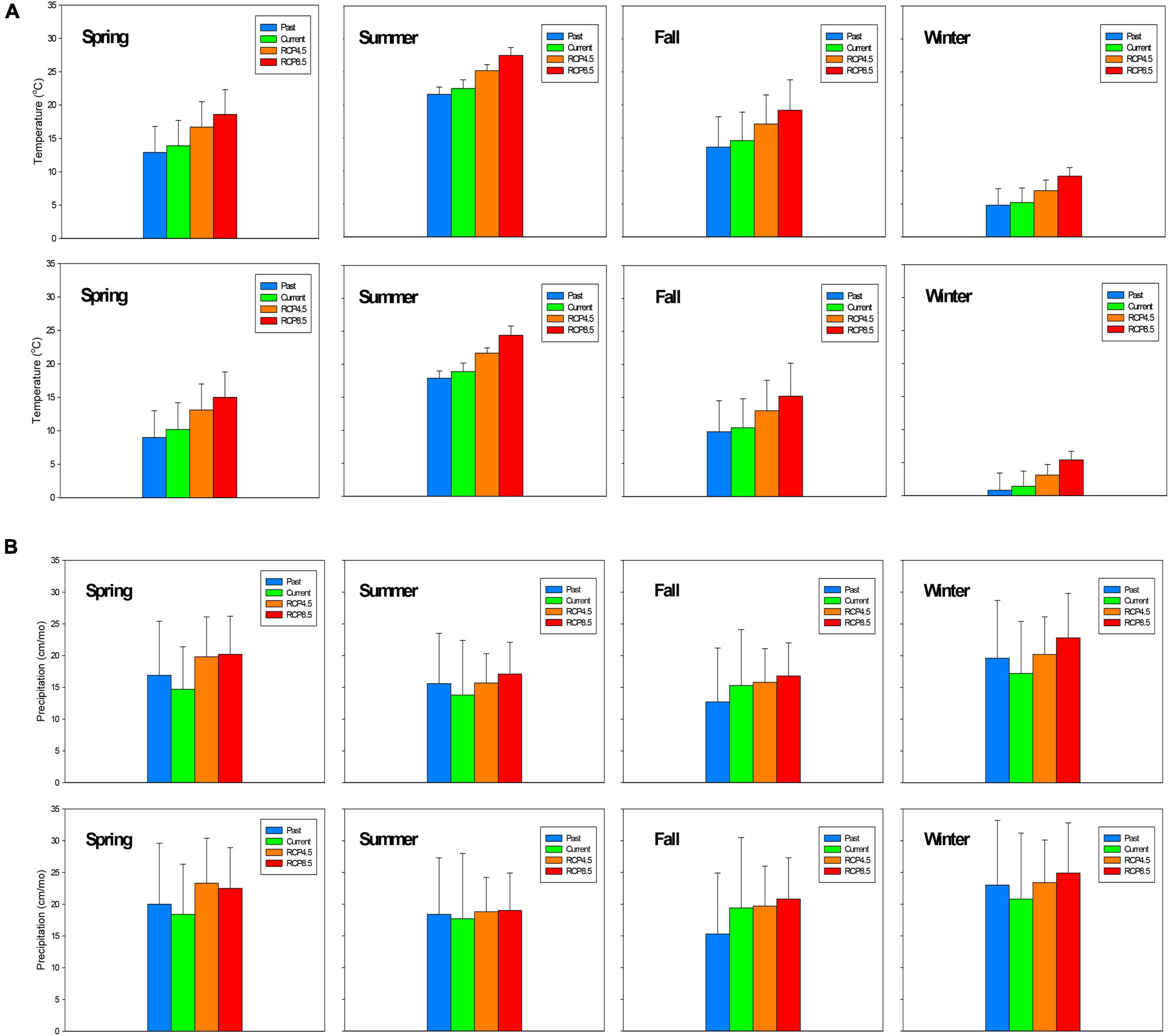
Figure 2. (A) Seasonal temperature comparison of past (1936–1965), current (1986–2015), and future (2071–2100) values for Watershed 18 (top) and Watershed 27 (bottom). (B) Seasonal precipitation comparison of past (1936–1965), current (1986–2015), and future (2071–2100) values at Watershed 18 (top) and Watershed 27 (bottom). Spring (March–May), summer (June–August), fall (September–November), and winter (December–February).

TABLE 1A

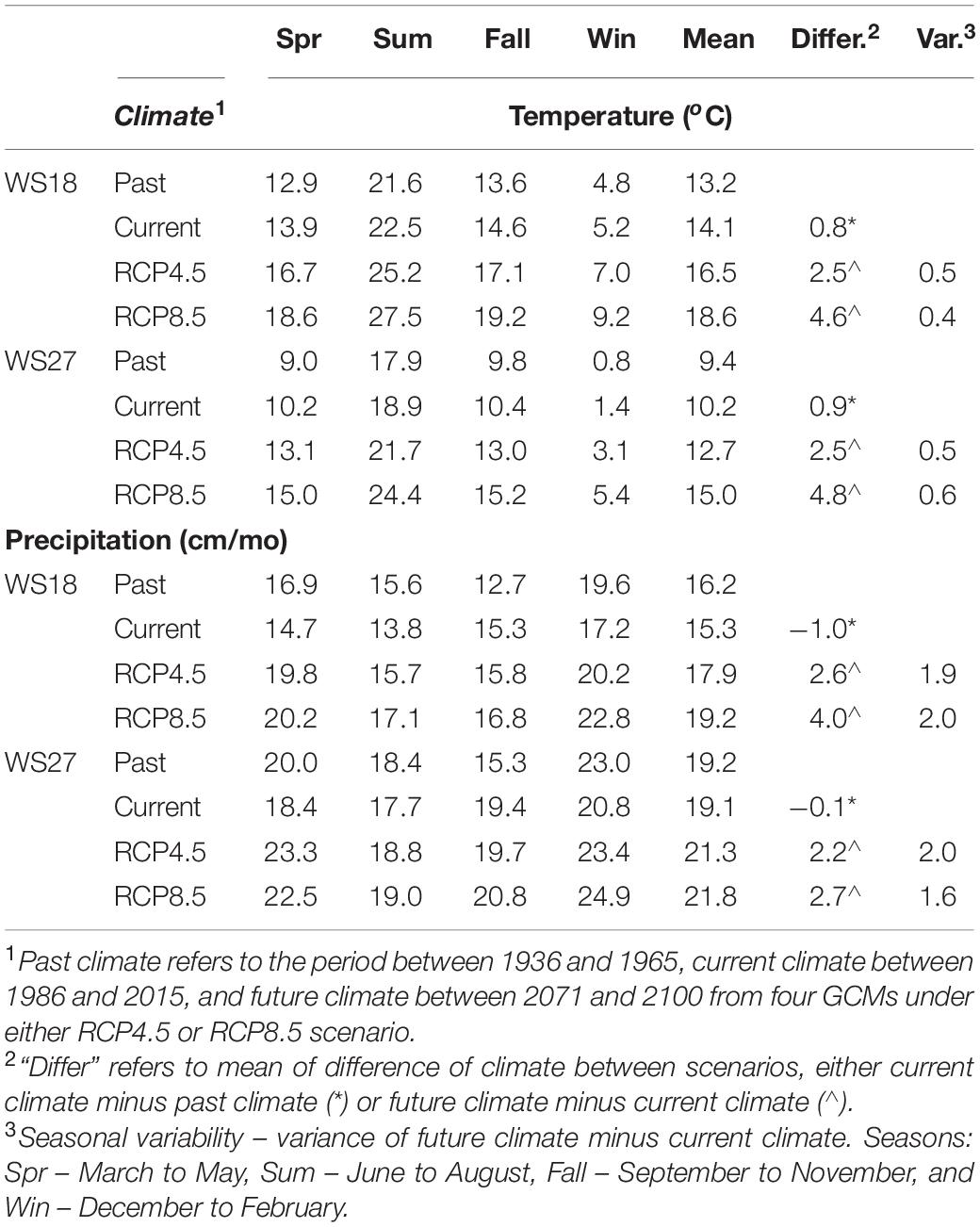
Table 1A. Seasonal temperature and precipitation in the past, current, and future (RCP4.5 and RCP8.5) conditions at WS18 and WS27.

Observed precipitation decreased from past to current conditions during all the seasons except for fall. In contrast, future precipitation is projected to increase ranging from 2.2 to 4.0 cm/mo in all seasons in the future compared to current conditions with the fall showing the smallest increment (Table 1). Both air temperature and precipitation projections for Coweeta follow a similar pattern of regional climate projections for the southeast U.S. (Intergovernmental Panel on Climate Change [IPCC], 2014). Noticeably, the temperature and precipitation projections for each season under changing climate scenario (2071–2100) are statistically significantly different from those under current climate scenario (1986–2015) (Table 1B).

TABLE 1B

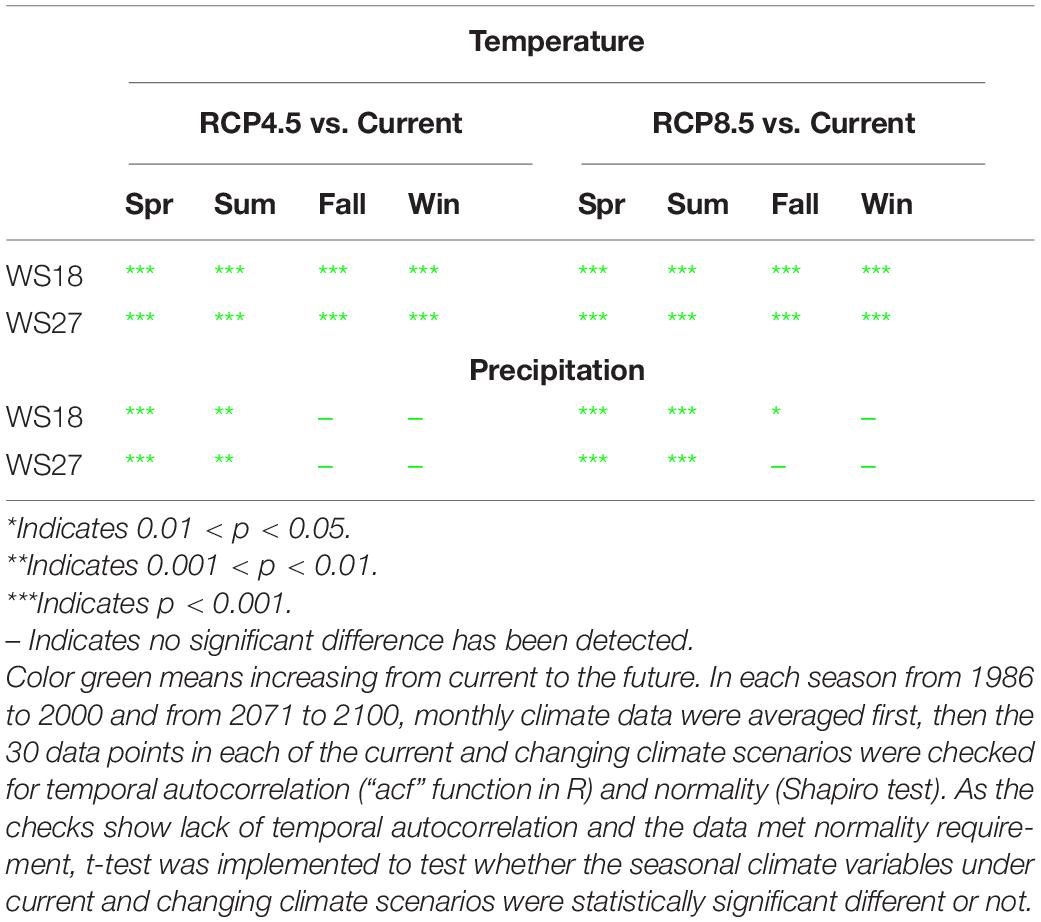
Table 1B. Statistical test of temperature and precipitation between current and changing climate scenarios.

Model Performance

The PnET-BGC mostly effectively simulated monthly and annual vegetation-soil-stream processes at both WS18 and WS27 based on the stream chemistry data from 1970s to 2014 and streamflow data from 1930s/1940 to 2014, with NME ranging from –0.06 to 0.09 (Table 2). However, NO₃^– was underestimated at both WS18 and WS27 and SO₄^2– was overestimated at WS18. The model also underestimated the variance of NO₃^– and SO₄^2–. Measured concentrations of SO₄^2– at WS18 showed an increase between 1980 and 1990s that are seemingly inconsistent with long-term decreases in atmospheric deposition of S during the same period after implementation of the Clean Air Act (1970) and Clean Air Act Amendments (1990) (USEPA⁷ accessed on 08/01/2020). However, this pattern may reflect desorption of soil SO₄^2– to streamwater that was absorbed during prior decades of elevated atmospheric S deposition (Rice et al., 2014). The nitrogen cycle is more complex than other element cycles and it strongly linked to processes of vegetation and microbial activities, and therefore, PnET-BGC simulation of stream NO₃^– involves larger uncertainties than other solutes (Fakhraei et al., 2016; Shao et al., 2020). In addition, contrary to a decrease in both observed nitrogen deposition and simulated nitrate leaching since the 1970s, both watersheds show an unexplainable increasing trend of observed nitrate concentration in streams, which the model does not reproduce.

TABLE 2

Table 2. Comparison of observed and simulated streamflow (unit: cm/month) and stream chemistry variables (unit: μmol/L) at WS18 and WS27.

In addition to the long-term observed streamflow and stream chemistry concentrations, our model simulations were consistent with other published observed data (Supplementary Table 3), including NPP, soil base saturation, and net nitrogen mineralization rate. Model simulated average aboveground NPPs at WS18 and WS27 between 1971 and 1980 are close to published data from Day and Monk (1977) (8,056 vs. 7,965 kg/ha-yr). For net nitrogen mineralization rate, the 10-year averages (1971–1980) are 2.5 and 3.1 mg N/kg soil-mo at WS18 and WS27, which are within the range reported by Knoepp and Swank (1998) based on the samples collected along an elevation gradient (<1.2 – 3.8 mg N/kg soil-mo), and consistent with the pattern that the highest values occur at elevations over 1,000 m. WS18 at the lower elevation has higher soil base saturation (BS) of 24.9% than higher elevation WS27 with a lower BS of 4.0% with simulated data from 2001 to 2010 (Supplementary Table 3). This simulated range is close to the data range obtained from USDA Forest Services in 2008 soil survey from 9.2 to 19.7%.

Principal Component Analysis

The PCA analysis indicated that the first three principal components explained ∼ 85% of variance of the 17 variables analyzed (Supplementary Tables 4, 5 and Figures 3, 4). Particularly, PC1 explained 63.2 and 68.8% of total variances under RCP4.5 and RCP8.5 respectively at WS 18. PC1s explained 50.6% and 57.1% of the variances under RCP4.5 and RCP8.5, respectively, at WS 27. Based on the eigenvectors, the first principal components (PC1s) represent the contrast between primary production and transpiration vs. soil and stream ANC, and the second principal components (PC2s) depict nitrogen mineralization rate. The third principal components (PC3s) represent the concentrations of sulfate in stream at WS18 under RCP4.5 and at WS27 under both RCP4.5 and RCP8.5, while the PC3 at WS18 under RCP8.5 represents streamflow.

FIGURE 3

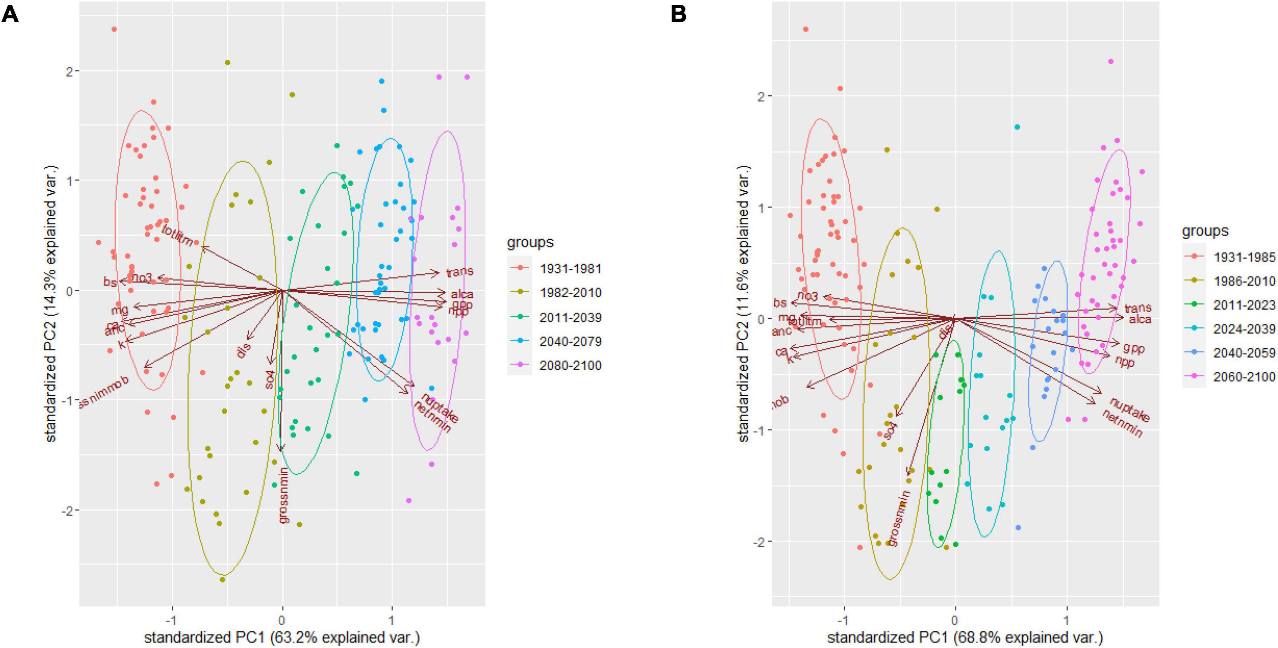
Figure 3. Principal component analysis (PCA) for the 17 variables at WS18 under RCP4.5 (A) and RCP8.5 (B). trans, transpiration; alca, ratio of Al and Ca in soil; gpp, gross primary productivity; npp, net primary productivity; nuptake, nitrogen uptake by vegetation; netnmin, net mineralization rate of nitrogen; grossnmin, gross mineralization rate of nitrogen; SO4, sulfate concentration in stream; dis, stream discharge; grossnimmob, gross immobilization rate of nitrogen; k, potassium concentration in stream; anc, acid neutralizing capacity; ca, calcium concentration in stream; mg, magnesium concentration in stream; bs, base saturation in soil; no3, nitrate concentration in stream; totlitm, total litter mass.

FIGURE 4

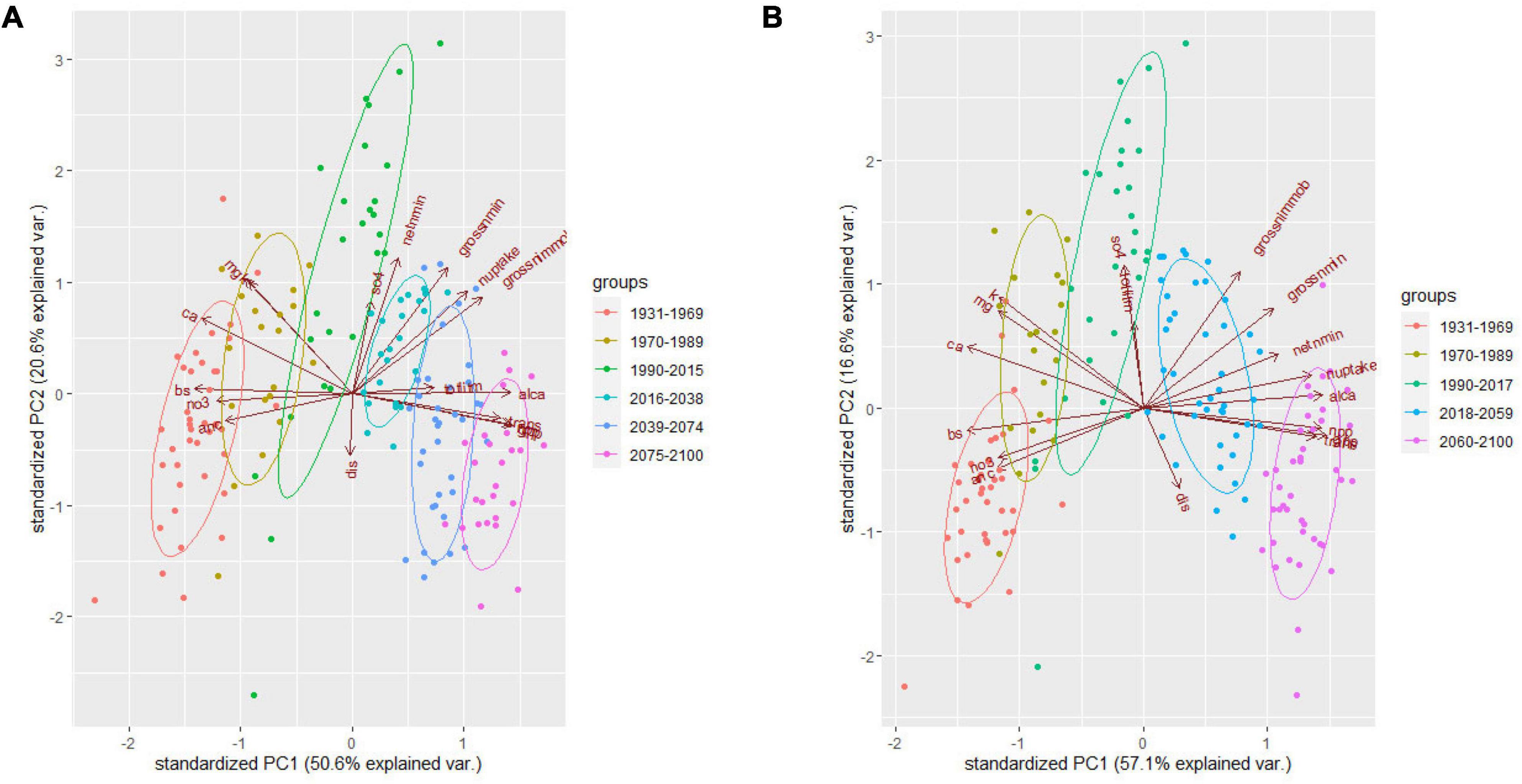
Figure 4. Principal component analysis (PCA) for the 17 variables at WS27 under RCP4.5 (A) and RCP8.5 (B). trans, transpiration; alca, ratio of Al and Ca in soil; gpp, gross primary productivity; npp, net primary productivity; nuptake, nitrogen uptake by vegetation; netnmin, net mineralization rate of nitrogen; grossnmin, gross mineralization rate of nitrogen; SO4, sulfate concentration in stream; dis, stream discharge; grossnimmob, gross immobilization rate of nitrogen; k, potassium concentration in stream; anc, acid neutralizing capacity; ca, calcium concentration in stream; mg, magnesium concentration in stream; bs, base saturation in soil; no3, nitrate concentration in stream; totlitm, total litter mass.

Seasonal Variability

Based on the PCA analysis, the evaluation of the impacts of climate change on watersheds of Coweeta focused on the processes that are important in PC1s and PC2s during different seasons. Particularly we focus on seasonal changes of transpiration, NPP, and stream ANC in the main text. The figures for other process variables are described in Appendix Figures (Supplementary Figures 1–7). As transpiration, GPP, and NPP are negligible in winter, the probability density distributions are very concentrated, unlike in other seasons.

For both watersheds, transpiration (Figure 5) is projected to increase under changing climate. However, the increase in transpiration at WS18 is smaller than at WS27, probably due to higher water stress. Even though transpiration increases, annual streamflow (Supplementary Figure 1) under future climate is projected to increase with increasing precipitation (26.8 and 32.7% at WS18 under RCP4.5 and 8.5; 11.9 and 14.7% for WS27 under RCP4.5 and 8.5, respectively). Seasonally, winter is the season that shows pronounced increase at both watersheds.

FIGURE 5

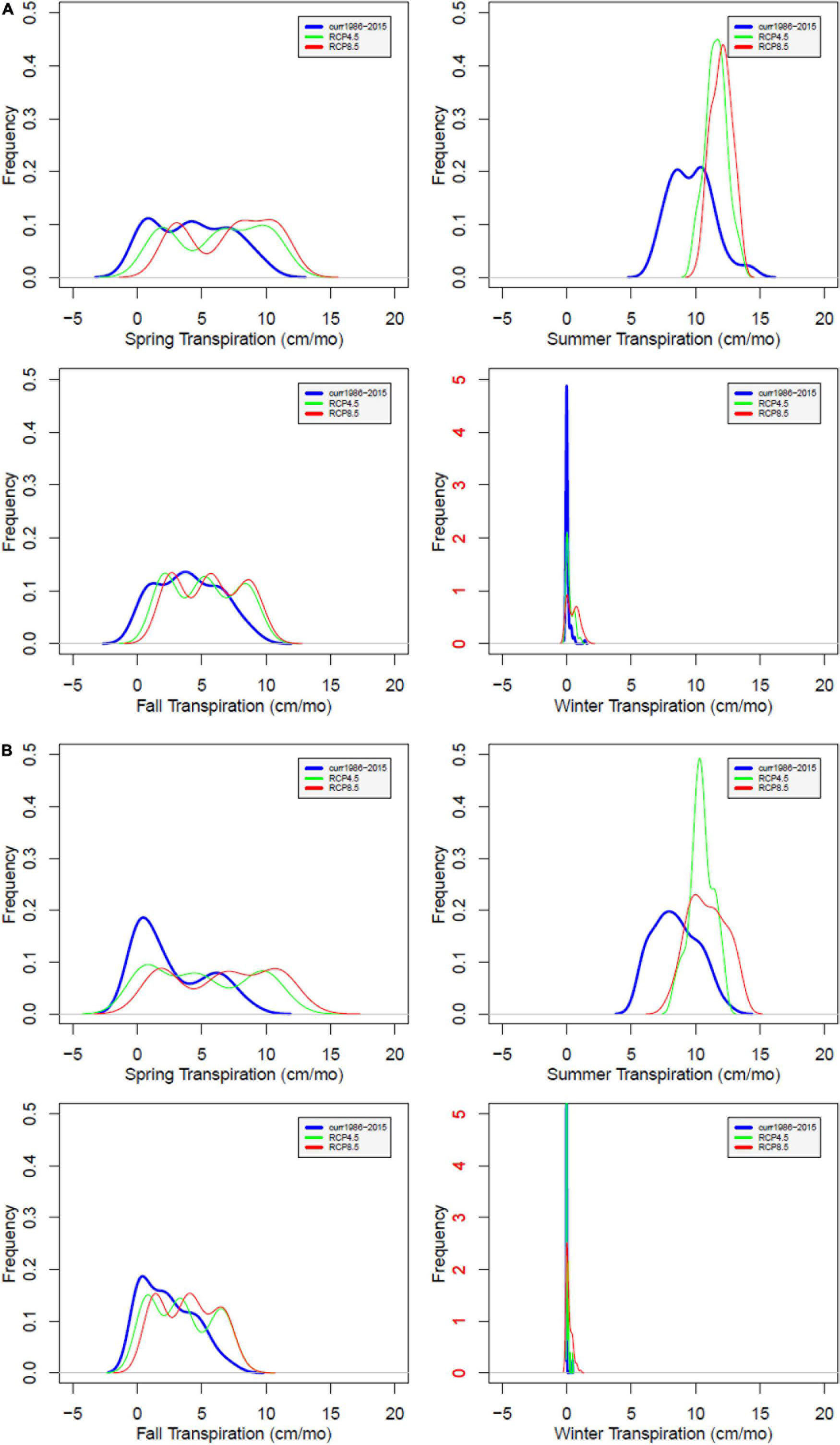
Figure 5. Probability distribution of simulated transpiration at WS18 (A) and WS27 (B) under future climate compared to values under current climate by season. Current (blue), RCP4.5 (green), and RCP8.5 (red). The red color of the labels in winter shows different range of y-axis compared to the other seasons.

The simulated impact of climate change on GPP is not as dramatic as for the water cycle (Supplementary Figure 2). However, it shows increases in spring and fall under both climate scenarios, increases in summer under RCP 4.5, but slight decrease under RCP 8.5. The increase of GPP at WS27 is more dramatic, especially in spring, summer and fall. Overall, annual GPP is projected to increase due to the extended growing season (2071–2100 compared to 1986–2015: increase by 13.8 and 17.9% for WS18, and 26.9 and 43.0% for WS27 under RCP4.5 and 8.5 scenarios, respectively). The simulated impact of climate change on NPP is moderate (Figure 6). On an annual basis, NPP is projected to increase although decreases are evident in the summer due to increases in respiration. Under RCP8.5, NPP shows decreases in summer and a larger variance in winter, with some high values. During summer, NPP is lowered in WS18 as much as 43.2 g biomass/m²-mo or 23.1% under RCP8.5. For WS27, simulated NPP increases during all seasons under RCP4.5. With RCP8.5, NPP shows decreases during summer. NPP is projected to increase to a greater degree in WS27 than WS18 due to less water stress associated with temperature increase.

FIGURE 6

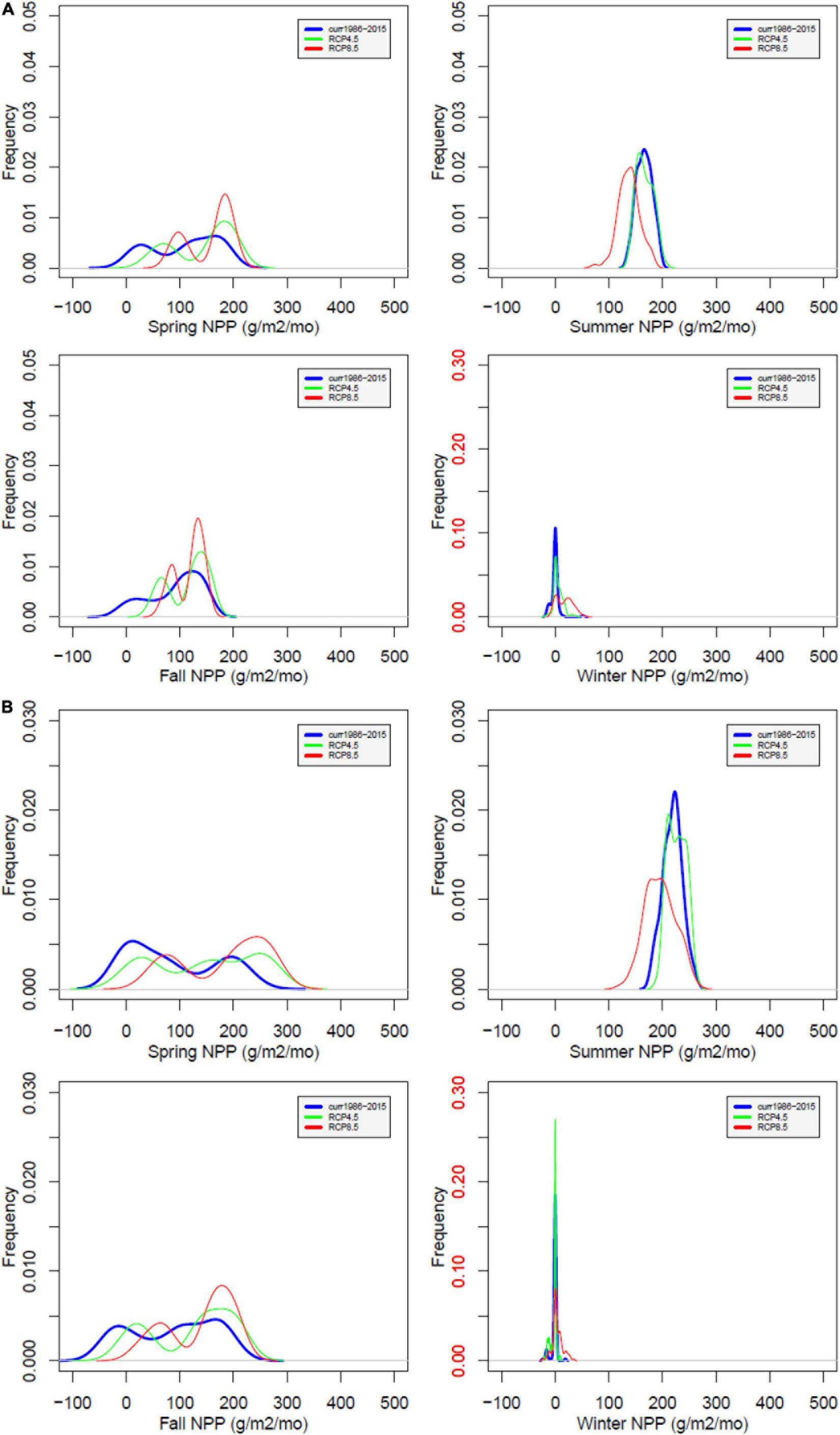
Figure 6. Probability distribution of simulated net primary productivity (NPP) at WS18 (A) and WS27 (B) under future climate compared to values under current climate by season. Current (blue), RCP4.5 (green), and RCP8.5 (red). The red color of the labels in winter shows different range of y-axis compared to the other seasons.

At WS18, stream ANC is projected to decrease during all seasons under future climate with the larger decrease under RCP 8.5 at WS18 (Figure 7). The impact of climate change on stream ANC is minimal at WS27, with small decreases under RCP8.5.

FIGURE 7

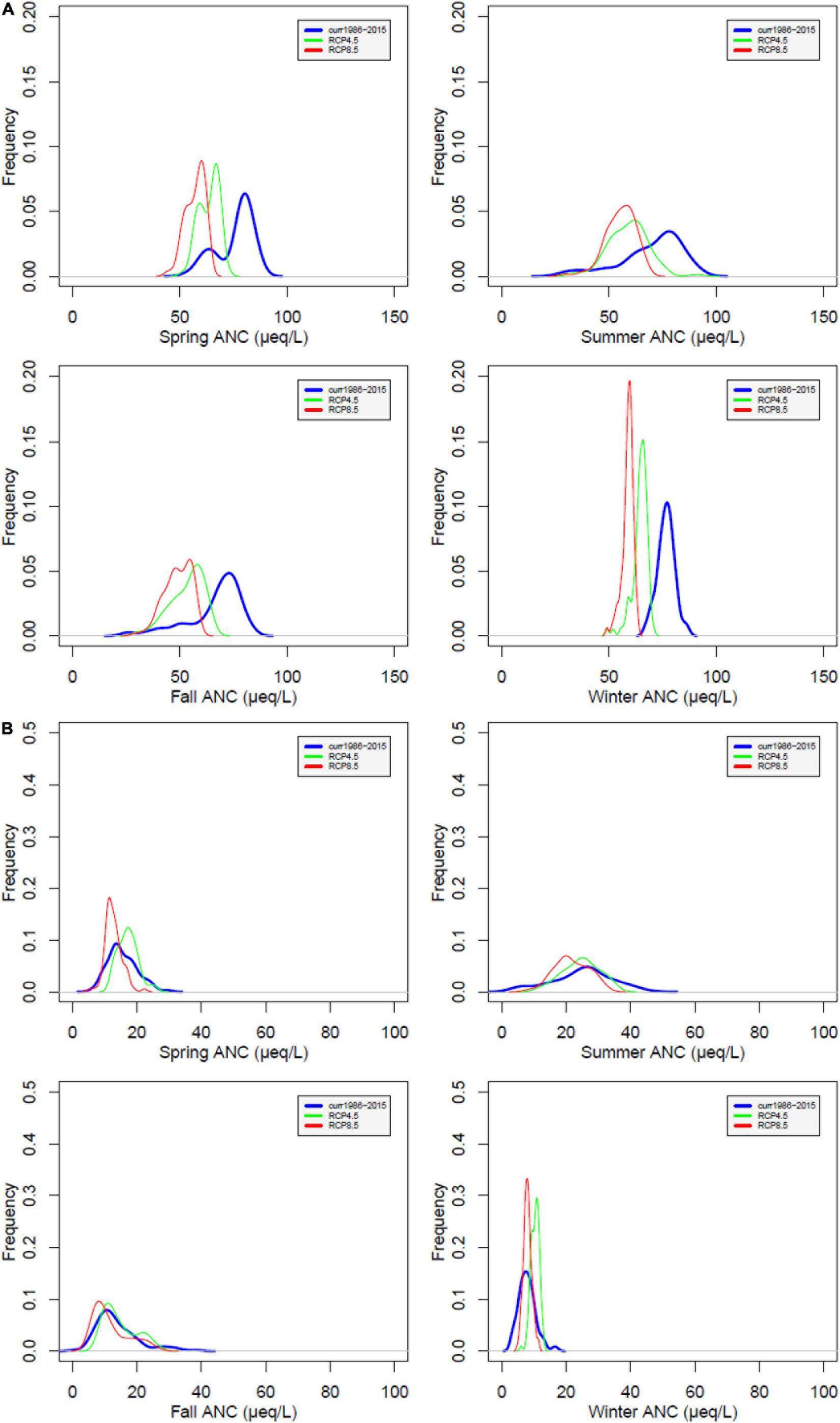
Figure 7. Probability distribution of simulated acid neutralizing capacity (ANC) at WS18 (A) and WS27 (B) under future climate compared to values under current climate by season. Current (blue), RCP4.5 (green), and RCP8.5 (red).

Under climate change, the most conservative element, Cl^–, as well as basic cations (Na⁺, K⁺, Ca²⁺, and Mg²⁺) and SO₄^2– exhibited decreases in concentration but increases in total flux associated with streamflow increases. The flux of the base cations in soil is mainly associated with release from wood litter. Calcium concentrations (Supplementary Figure 3) in streamwater decrease dramatically in all seasons at WS18. A similar decrease is also evident in WS27, but not as marked. Potassium concentrations decrease (Supplementary Figure 4) in stream water during all seasons at WS18 with the most distinct change occurring in winter and spring. Decreases in potassium are also evident at WS27 in all seasons with the most distinct change occurring in winter. Sulfate concentration (Supplementary Figure 5) in stream water decreases in both watersheds, especially in winter under RCP8.5 and with lower values than projected under RCP4.5 at WS18. Compared to the conditions under current climate, future sulfate concentration will be less varied at WS27 but showing more distinct change than at WS18. WS18 has the highest median sulfate concentration in summer while at WS27, the highest concentrations occur in fall and winter.

Soil processes and properties are predicted to change as well, including soil base saturation, Al:Ca concentration in soil, and nitrogen mineralization rate. Soil base saturation is indicative of the soil acid-base status with lower values symptomatic of more acidic soil. High concentrations of Al:Ca in soil can be toxic to biota.

Soil base saturation (Supplementary Figure 6) shows decreases during all the seasons at both watersheds under RCP4.5 and 8.5. Decreases are pronounced under both climate scenarios at WS18, but only marginally under RCP8.5 at WS27. Al:Ca in soil shows a dramatic increase in all the seasons, but increases are most pronounced during summer at WS18 under RCP4.5 and 8.5. Al:Ca in soil increases particularly during summer at WS27. The simulated impact of climate change on N mineralization is small (Supplementary Figure 7). In WS18 under RCP8.5, the N mineralization rate shows some decrease. At WS27, the mineralization shows some decrease in winter but increase in summer.

Overall, the response of individual forest processes to climate change varies by season. Furthermore, vegetation seems to be more sensitive to climate change at WS27 than WS18, while soil processes and stream chemistry seem to be more impacted by climate change at WS18 than at WS27.

To more comprehensively present the impact of climate change, we summarized the changes of the 17 model-derived key watershed process variables in each season between current (1986–2015) and future (2071–2100) for both RCP4.5 and 8.5 scenarios, particularly, the directions of the changes and the significance levels of the statistical tests (Table 3).

TABLE 3

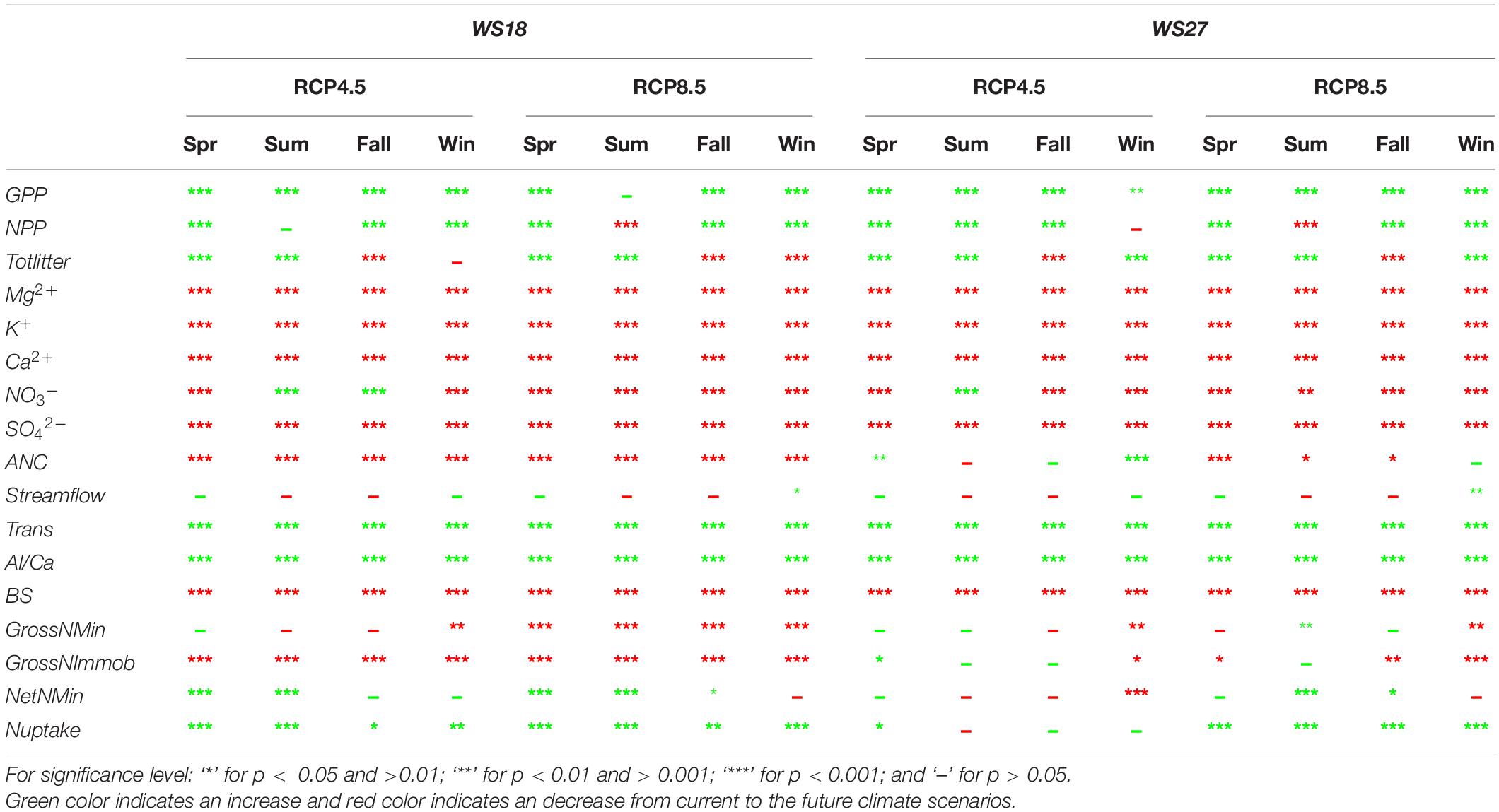
Table 3. Significance test of 17 watershed state variables between current (1986–2015) and future (2071–2100) for the two studied watersheds (GPP, Gross Primary Productivity; NPP, Net Primary Productivity; Totlitter, Total litter produced; ANC, Acid Neutralizing Capacity; Trans, Transpiration; BS, Base Saturation; GrossNMin, Gross Nitrogen mineralization rate; GrossNImmob, Gross Nitrogen Immobilization rate; NetNMin, Net Nitrogen mineralization rate; Nupdate, Nitrogen uptake rate).

In the vegetation processes, GPP and NPP are predicted to increase significantly except summer under RCP8.5. This can be explained by higher water stress during this season.

In the hydrology process, transpiration will significantly increase during almost all seasons as both precipitation and temperature are projected to increase from present day to the end of this century. Streamflow at the Coweeta basin is trending to increase in winter and spring seasons and decrease in summer and fall seasons, but the predictions in the future are not significantly different from current conditions except winter under RCP8.5.

The soil processes captured in base saturation across both watersheds and seasons are predicted to significantly decrease, which indicates a greater loss of base cations from the soil under changing climate. Along with the reduction of base saturation, the Al:Ca ratio is predicted to increase at all seasons under both climate scenarios, and the increase is statistically significant in all seasons. Additionally, some nitrogen processes are negatively impacted, such as gross nitrogen mineralization and immobilization. For the net nitrogen mineralization, results are complicated due to counteracting processes being involved at the same time.

In streamwater chemistry, the concentrations of major cations and sulfate are predicted to significantly decrease, even though soil losses of cations to nearby water flows (streams) are predicted to increase, probably due to the higher streamflow. ANC shows significant decrease in four seasons at WS 18 under both climate change scenarios and spring, summer, and fall at WS 27 under RCP8.5. The change of nitrate concentration mostly shows decrease.

We also found broad-scale climatic variability like El Niño-Southern Oscillation (ENSO) affected seasonal biogeochemical processes. Oceanic Niño Index (ONI that indicates ENSO) had a negative relation with the integrated biogeochemical processes (PC1) in the winter and early spring (January to April) at WS18 and WS27 (Supplementary Figure 8). Strong El Niño years generally had lower PC1 (Supplementary Figures 8, 9), indicating lower productivity and higher ANC in soil and streams, probably due to lower temperature in winter-early spring.

Temporal Trend of Biogeochemical Processes and Change Points

From the time series of the scores of the PC1s that explained more than 50% of the total variances, we derived five similar decadal change points for WS 18 and 27 (Table 4 and Figure 8). The change points occurred earlier at WS18 than at WS27 during 1980s and 2010s but are projected to occur at similar time points or even earlier at WS 27 relative to WS18 under future changing climate. This shift may imply that future climate might accelerate changes of biogeochemical processes at the higher-elevation WS27 site. The last change points are predicted to occur 20 years earlier under RCP8.5 (2059 at WS18 and WS27) compared to those under RCP4.5 (2079 at WS18 and 2074 at WS27) at the lower- and higher-elevation forests, respectively. The groups based on the time of change points of the PC1s confirmed their validity due to minimum overlaps between these different groups (Figures 3, 4).

TABLE 4

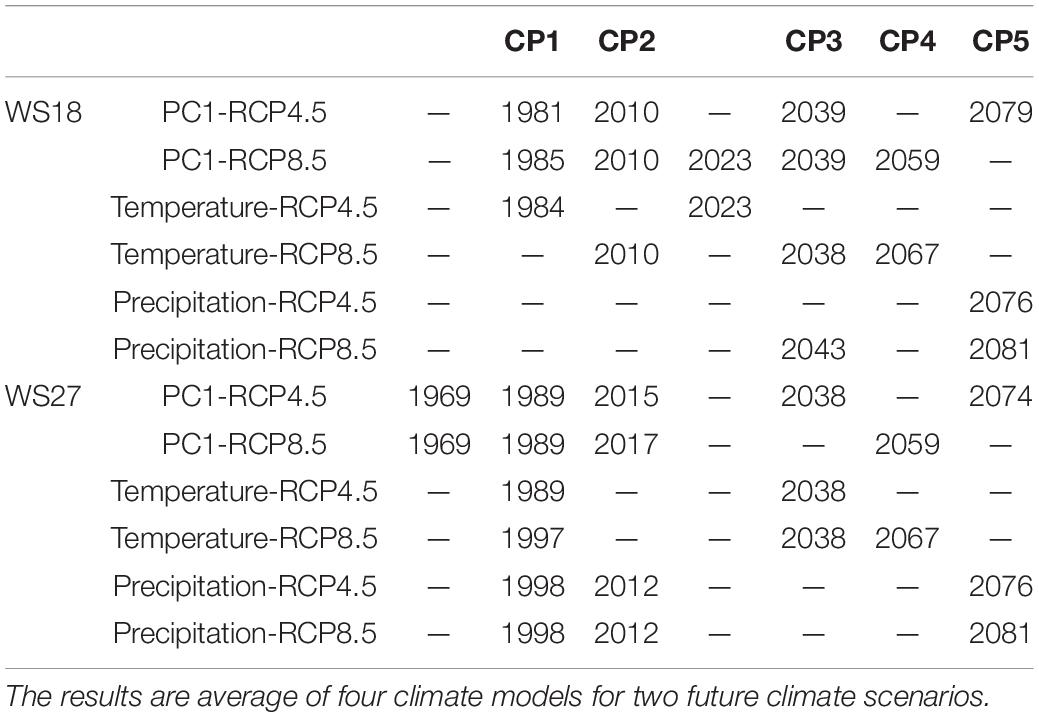
Table 4. Change points of the scores of the first principal components (PC1s) and climate (temperature and precipitation).

FIGURE 8

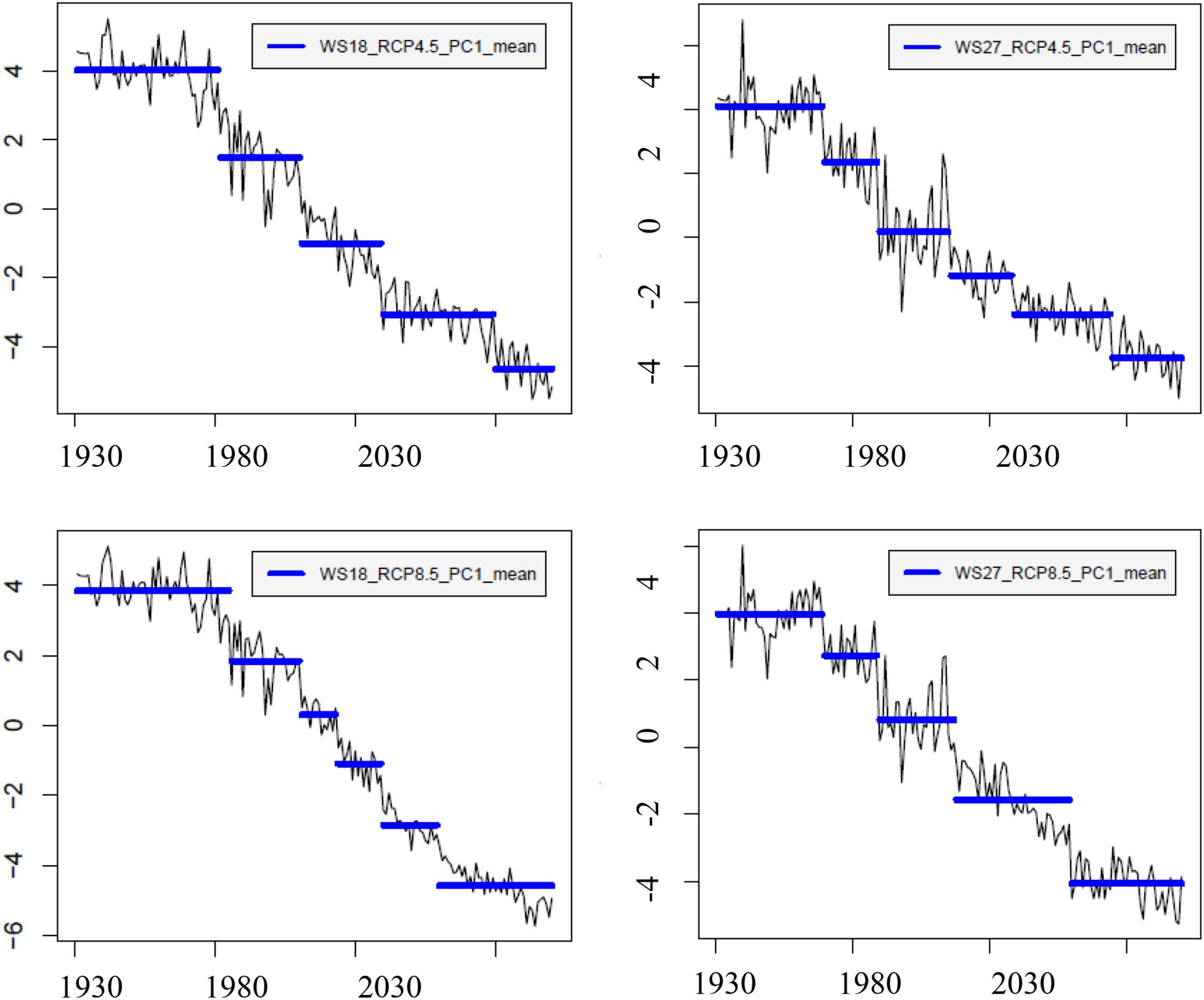
Figure 8. Change points of the first principle component of the simulated biogeochemical variables at WS18 and WS27 (top left – WS18 RCP4.5, bottom left – WS18 RCP8.5, top right – WS27 RCP4.5, and bottom right – WS27 RCP8.5).

When we compared the change points of temperature and precipitation to those of PC1, we found the first few change points of PC1 matched those of temperature at WS18, implying temperature change is likely an important driver of watershed response (Table 4 and Supplementary Figure 10). However, precipitation change appears to be the main driver for the change points of PC1 in 2079 at WS18. At WS27, precipitation is likely the main driver for the change points in 2010s and the 2070s, while temperature is the main driver for the change points in 1989, 2030s and around 2060. The climatic driver is not clear for the change point in 1969. In general, the last change points of PC1 under RCP4.5 (2070s) at both watersheds are likely driven by precipitation, while they seem to be driven by temperature under RCP8.5 (2050s–2060s).

Discussion

Spatial and Seasonal Variability

In this analysis, we found vegetation is affected by climate change more at the higher elevation than at lower elevation, consistent with Lamprecht et al. (2018). The impacts of climate change on the hydrochemical processes have shown large spatial variability. Evapotranspiration and streamflow are predicted to increase under both moderate (RCP4.5) and high-end (RCP8.5) climate change scenarios at both WS18 and WS27. The predicted increase of evapotranspiration with climate change is consistent with patterns found in seven forest watersheds across four northeastern states in the United States (Pourmokhtarian et al., 2017). Annual streamflow, however, is highly variable among these watersheds, with some watersheds predicted to increase while others predicted to decrease, depending on whether the increase of evapotranspiration is offset by the increase of precipitation (Campbell et al., 2011). The hydrological predictions are different at the Andrews Experimental Forest in the northwestern U.S., where it is predicted that there will be a 20–71% decrease in annual transpiration under future climate change corresponding to 49–86% decreases in foliar biomass due to drought stress (Dong et al., 2019). The decrease in evapotranspiration could contribute to higher streamflow at this forest. In the western U.S. where future climate is projected to become warmer and dryer, gross and net nitrogen mineralization are predicted to increase, and NPP is also predicted to increase, due to feedbacks between warmer temperatures and enhanced nitrogen mineralization in forests. In the Coweeta Basin, Knoepp and Swank (1998, 2002) found that temperature and temperature-moisture interactions significantly affected net soil nitrogen mineralization based on a series of long-term studied plots at different elevations. When temperature was warmer and soil moisture content was higher, nitrogen mineralization was reported to be greater, consistent with our findings (Table 3). From the relatively low elevation oak-pine dominated watershed to the higher elevation watershed dominated by northern hardwoods, net nitrogen mineralization rate showed a strong spatial pattern with the highest rate observed at the highest elevation site, even though other factors (e.g., C:N ratio in soil) besides temperature and soil moisture influenced soil nitrogen processes both in the laboratory and in situ.

Climate change is projected to have variable effects on ecosystem responses across the seasons. Even though annual streamflow is projected to increase, these increases are less pronounced in the growing season. Spring may be impacted substantially because of loss of snowpack (Reinmann et al., 2018) and early leaf-out timing that can extend the growing season and exacerbate drought stress. A hotter summer together with a warmer spring, coupled with temporally unevenly distributed precipitation, could increase drought stress and risks of wildfire (Table 3). The drought stress could extend to other seasons. The fall season presents the lowest percent increase of precipitation among all the seasons. With higher evapotranspiration driven by higher temperature, streamflow is projected to decrease thereby causing more droughts. During winter, relative temperature (three times greater at WS27 in winter under RCP8.5) increases are particularly pronounced, which decreases precipitation inputs as snow and the magnitude and duration of snow coverage (Table 1A, Campbell et al., 2011; Pourmokhtarian et al., 2017).

Effects of climate change are difficult to evaluate during the “shoulder seasons” due to the large year to year variability. As a result, impacts during these periods are generally ignored, however, more and more research shows transitional seasons are affected by climate change to a greater degree than previously thought (Xie et al., 2015; Goss et al., 2020). Traditional definition of seasons and transition between seasons are predicted to become less clear as we may experience shorter spring and fall, while winter and summer will become longer, and most of the year will fall into more extreme hot and cold temperatures (Thomson, 2009). The impact of climate change on biogeochemical process during the shoulder transitions needs to be studied further.

The Impact of CO₂ on Ecosystems

Elevated CO₂ associated with climate change tends to increase plant WUE, i.e., increases primary productivity and reduces evapotranspiration (Reyer et al., 2015), which benefits forests by increasing their drought tolerance although there are counteracting effects to consider. Elevated CO₂ could also increase plant leaf area, therefore, making trees less drought tolerant (Ghannoum and Way, 2011). Reduced evapotranspiration could also lead to increases in leaf temperature, thereby increasing temperature stress. Increased productivity under elevated CO₂ may increase litter (Hyvonen et al., 2007), leading to increased litter accumulation (if decomposition cannot catch up) and higher vulnerability to fire. Many studies on the response of forest habitats to increased CO₂ are made at the small scale of individual trees or small plots. Scaling up the effect to the ecosystem scales involves considerable uncertainty. Furthermore, the fertilization effect of CO₂ is commonly found only in young trees (Korner et al., 2007). In our study, we assume elevated CO₂ increases primary productivity at the entire watershed without considering other counteracting effects (e.g., leaf temperature increase or age of trees), therefore our prediction of primary productivity under climate change is likely an optimistic estimate.

Uncertainties of Model Predictions

It is important to predict climate as accurate as possible in order to make valid predictions of ecosystem function change. This has been facilitated using downscaling method in our study. However, broad-scale climate variability like ENSO may enhance changes in temperature or precipitation (El Niño and La Niña Years and intensities at⁸ and accessed on 08/01/2020) at local spatial scales, and therefore has impact on biogeochemical processes as what we found out in this study. Generally, during El Niño years, the southeastern U.S. experiences cooler temperatures and wetter conditions in winter-early spring⁹ accessed on 08/01/2020. Together with the North Atlantic Oscillation (NAO), it was found that the southern Appalachians have higher snowfall and cooler temperature in winter during El Niño and negative NAO phases (Eck et al., 2019). In contrast, La Niña and positive NAO years result in warmer and drier winter weather. As the prediction of El Niño’s intensity using current climate models involves large uncertainty (Wang et al., 2019), predictions of temperature, precipitation and biogeochemical processes are particularly challenging under climate change. In order to reduce uncertainties of predicted biogeochemical processes, broad-scale climate variability needs to be accounted for in the climate change models.

PnET-BGC is a watershed-scale model that is operated on a monthly time step, so it is not well suited to address finer spatial and temporal resolutions (Merganicova et al., 2019). This model treats the vegetation in the watershed as a big leaf, therefore, it does not consider the difference among tree types and fine structures (Elliott et al., 2015), adaption (Jandi et al., 2019), or explicitly accounts for shift of vegetation types. Previous studies show that the critical transitions of vegetation type in mountain forests (Reich et al., 1995; Albrich et al., 2020) may change the fundamental relationships between foliar N concentration and maximum photosynthesis rate, which is one of the two fundamental relations that PnET-BGC is built on (Gbondo–Tugbawa et al., 2001). Furthermore, the function of understory shrub vegetation in cycling nutrients, carbon, and water (Rothstein, 2000) is another component not considered in this model. Different stages of vegetation not only have different capabilities of nutrient uptake, photosynthesis, cycling of carbon and water, but larger and older trees may be also more susceptible to stress such as drought and storms (Clinton et al., 1993, 2003; Clinton and Baker, 2000), which is not depicted in the model.

This PnET-BGC model requires a number of empirical data to calibrate, some of which are not available for the study watersheds (such as Al and DOC concentrations), making calibration for these parameters less robust. In addition, the model under-predicts nitrate concentrations in streamwater, suggesting the need to critically review this submodule for applications at Coweeta watersheds. Other simulations using PnET-BGC have been challenged to accurately simulate nitrogen dynamics (e.g., Shao et al., 2020). This model is designed to predict long-term hydrologic and biogeochemical function at the watershed scale (Aber and Federer, 1992; Gbondo–Tugbawa et al., 2001), combined with the lack of feedback between vegetation and climate, it is not an ideal tool to derive regime shifts. Other components lacking in the PnET-BGC further contribute to uncertainties in the simulations. These include the lack of multiple soil depths (two-layer model available but harder to calibrate so we used one-layer model), and lack of consideration of phosphorus dynamics.

Despite these aspects that can be improved, PnET-BGC provides a useful tool to evaluate the impact of climate change on forested ecosystems over long time scales (multiple decades to centuries). When depicting complex ecosystems, as many other ecological models have done, it is necessary to make assumptions and acknowledge inherent uncertainties (Aber and Federer, 1992). In order to capture the uncertainty, we have applied two climate change scenarios. The consistent response of biogeochemical cycles provides higher confidence in our predictions on the climate change impact.

Implications for Forest Management

This research will provide useful information for resource managers in anticipation of the potential risks forests may face under climate change. Forest managers can consider possible measures such as tree planting and forest restoration, wildfire control, establishment of mixed stands, planting better adapted species or varieties to mitigate adverse impacts in the future. For monitoring, the forest managers may consider watershed specific and seasonal specific evaluations instead of focusing on growing seasons or one process in soil or vegetation only.

We are facing an uncertain future based on (1) the greater uncertainty in prediction for precipitation than for temperature (Intergovernmental Panel on Climate Change [IPCC], 2014), and (2) precipitation will be the main driver for future change points under RCP4.5. Considering the change that may occur in high-elevation forests directly influences ecosystems downslope and downstream and the highly uncertain future projections, measures should be taken to protect, conserve and restore these high-elevation forests. The improved understanding of forests’ non-linear responses to a changing environment gained from this research can potentially guide decisions in forest management even with large uncertainties, for example, detection of early warning signs of potential regime shifts and selection of species planted in restoration.

Conclusion

We predict both positive and negative impacts of climate change on hydrochemical processes, for example, we predict increases in acidification of soil and streamwater despite an increase in primary productivity under climate change. The predicted hydrochemical changes show strong seasonal variability depending on biogeochemical processes. We also find climate change will likely have a greater impact on soil processes at the lower elevation watershed and on vegetation processes at the higher elevation watershed. The change-point analysis suggests biogeochemical cycles in vegetation, soil, and streams may be accelerating at higher-elevation. These findings that include integrated hydrochemical processes in temporal and spatial (lower-elevation vs. higher-elevation) contexts provide multi-dimensional metrics that can be used in part or as a whole by southern forest managers to evaluate the benefits and disadvantages in anticipation of future climatic change to improve the resilience of forest ecosystems and downstream surface water in the future. Additionally, the integrated modeling framework can be applied to specific management practice scenarios of interest to yield more detailed quantitative predictions for in-depth analysis of these management plans.

Data Availability Statement

The original contributions presented in the study are included in the article/Supplementary Material, further inquiries can be directed to the corresponding author/s.

Author Contributions

KE and CM provided measured data at the Coweeta Basin. HH performed the PnET-BGC model runs with the guidance of WW and CD. HH and WW interpreted the model results and wrote the first draft of the manuscript. All authors commented on previous versions, and read and approved the final manuscript.

Funding

Funding for this study was provided by U.S. Environmental Protection Agency through the STAR program (R834188) and Department of Chemistry at the University of Southern Mississippi through teaching assistantship to HH.

Conflict of Interest

The authors declare that the research was conducted in the absence of any commercial or financial relationships that could be construed as a potential conflict of interest.

Publisher’s Note

All claims expressed in this article are solely those of the authors and do not necessarily represent those of their affiliated organizations, or those of the publisher, the editors and the reviewers. Any product that may be evaluated in this article, or claim that may be made by its manufacturer, is not guaranteed or endorsed by the publisher.

Acknowledgments

We would like to thank Katherine Hayhoe and her research group to provide downscaled climate change data at the Coweeta Basin. Data for model calibration and validation were provided by the Coweeta Hydrological Laboratory. We particularly would like to thank J. Knoepp for the soil data and valuable insights and discussions on the forest processes at the Coweeta Basin. We would also like to thank P. Biber, D. Dillon, and R. Leaf for critical comments on Huang’s dissertation, one chapter of which further develops into this manuscript.

Supplementary Material

The Supplementary Material for this article can be found online at: https://www.frontiersin.org/articles/10.3389/ffgc.2022.853729/full#supplementary-material

Footnotes

1. ^ https://www.un.org/en/observances/forests-and-trees-day
2. ^ https://www.srs.fs.usda.gov/coweeta/tools-and-data/
3. ^ http://nadp.slh.wisc.edu/
4. ^ https://www.epa.gov/castnet
5. ^ http://nadp.slh.wisc.edu/data/ntn/plots/ntntrends.html?siteID=NC25
6. ^ https://ctdrisco.expressions.syr.edu/pnet-bgc-model/
7. ^ https://www.epa.gov/clean-air-act-overview/evolution-clean-air-act
8. ^ https://ggweather.com/enso/oni.htm
9. ^ https://www.weather.gov/tae/enso

References

Aber, J. D., and Federer, C. A. (1992). A generalized, lumped–parameter model of photosynthesis, evapotranspiration and net primary production in temperate and boreal forest ecosystems. Oecologia 92, 463–474. doi: 10.1007/BF00317837

PubMed Abstract | CrossRef Full Text | Google Scholar

Albrich, K., Rammer, W., and Seidl, R. (2020). Climate change causes critical transitions and irreversible alterations of mountain forests. Glob. Change Biol. 26, 4013–4027. doi: 10.1111/gcb.15118

PubMed Abstract | CrossRef Full Text | Google Scholar

Anderson, T., Carstensen, J., Hernandez–Garcia, E., and Duarte, C. M. (2009). Ecological thresholds and regime shifts: approaches to identification. Trends Ecol. Evol 24, 49–57. doi: 10.1016/j.tree.2008.07.014

PubMed Abstract | CrossRef Full Text | Google Scholar

Both, A. J., Mears, D. R., Reiss, E., and Roberts, W. J. (2002). Floor heating in greenhouses. Horticult. Eng. 17:8.

Google Scholar

Campbell, J. L., Driscoll, C. T., Pourmokhtarian, A., and Hayhoe, K. (2011). Streamflow responses to past and projected future changes in climate at the Hubbard Brook Experimental Forest, New Hampshire, United States. Water Resour. Res 47:W02514. doi: 10.1029/2010WR009438

CrossRef Full Text | Google Scholar

Center for Climate and Energy Solutions [C2ES] (2019). Climate Essentials – Science and Impacts. Arlington: Center for Climate and Energy Solutions.

Google Scholar

Chen, L., and Driscoll, C. T. (2004). Modeling the response of soil and surface waters in the Adirondack and Catskill regions of New York to changes in atmospheric deposition and historical land disturbance. Atmos. Environ. 38, 4099–4109. doi: 10.1016/j.atmosenv.2004.04.028

CrossRef Full Text | Google Scholar

Chen, L., and Driscoll, C. T. (2005a). Regional application of an integrated biological model to northern New England and Maine. Ecol. Appl. 15, 1783–1797. doi: 10.1890/04-1052

CrossRef Full Text | Google Scholar

Chen, L., and Driscoll, C. T. (2005b). Regional assessment of the response of the acid–base status of lake watersheds in the Adirondack region of New York to changes in atmospheric deposition using PnET–BGC. Environ. Sci. Technol. 39, 787–794. doi: 10.1021/es049583t

PubMed Abstract | CrossRef Full Text | Google Scholar

Chen, L., Driscoll, C. T., Gbondo–Tugbawa, S., Mitchell, M. J., and Murdoch, P. S. (2004). The application of an integrated biogeochemical model (PnET–BGC) to five forested watersheds in the Adirondack and Catskill regions of New York. Hydrol. Process 18, 2631–2650. doi: 10.1002/hyp.5571

CrossRef Full Text | Google Scholar

Clinton, B. D., and Baker, C. R. (2000). Catastrophic windthrow in the southern Appalachians: characteristics of pits and mounds and initial vegetation responses. Forest Ecol. Manag. 126, 51–60. doi: 10.1016/S0378-1127(99)00082-1

CrossRef Full Text | Google Scholar

Clinton, B. D., Boring, L. R., and Swank, W. T. (1993). Characteristics of canopy gaps and drought influences in oak forests of the Coweeta Basin. Ecology 74, 1551–1558. doi: 10.2307/1940082

CrossRef Full Text | Google Scholar

Clinton, B. D., Yeakley, A., and Apsley, D. K. (2003). Tree growth and mortality in a Southern Appalachian deciduous forest following extended wet and dry periods. Gastanea 68, 189–200.

Google Scholar

Conant, R. T., Ryan, M. J., Agren, G. I., Birge, H. E., Davidson, E. A., Eliasson, P. E., et al. (2011). Temperature and soil organic matter decomposition rates–synthesis of current knowledge and a way forward. Glob. Change Biol. 17, 3392–3404. doi: 10.1111/j.1365-2486.2011.02496.x

CrossRef Full Text | Google Scholar

Davidson, E. A., and Janssens, I. A. (2006). Temperature sensitivity of soil carbon decomposition and feedbacks to climate change. Nature 440, 165–173. doi: 10.1038/nature04514

PubMed Abstract | CrossRef Full Text | Google Scholar

Day, F. P. Jr., and Monk, C. D. (1977). Net primary production and phenology on a southern Appalachian watershed. Am. J. Bot. 64, 1117–1125. doi: 10.2307/2442168

CrossRef Full Text | Google Scholar

Day, F. P. Jr., Philips, D. L., and Monk, C. D. (1988). “Forest communities and patterns,” in Forest Hydrology and Ecology at Coweeta Ecological Studies, Vol. 66, eds W. T. Swank and D. A. Crossley Jr. (New York, NY: Springer–Verlag), 141–149. doi: 10.1007/978-1-4612-3732-7_10

CrossRef Full Text | Google Scholar

Day, P. Jr., and Monk, C. D. (1974). Vegetation patterns on a southern Appalachian watershed. Ecology 55, 1064–1074. doi: 10.2307/1940356

CrossRef Full Text | Google Scholar

Delpla, I., Jung, A. V., Baures, E., Clement, M., and Thomas, O. (2009). Impacts of climate change on surface water quality in relation to drinking water production. Environ. Int. 35, 1225–1233. doi: 10.1016/j.envint.2009.07.001

PubMed Abstract | CrossRef Full Text | Google Scholar

Dong, Z., Driscoll, C. T., Johnson, S. L., Campbell, J. L., Pourmokhtarian, A., Stoner, A. M. K., et al. (2019). Projections of water, carbon, and nitrogen dynamics under future climate change in an old–growth Douglas–fir forest in the western Cascade Range using a biogeochemical model. Sci. Total Environ. 656, 608–624. doi: 10.1016/j.scitotenv.2018.11.377

PubMed Abstract | CrossRef Full Text | Google Scholar

Driscoll, C. T., Lawrence, G. B., Bulger, A. J., Butler, T. J., Cronan, C. S., Eagar, C., et al. (2001). Acidic deposition in the northeastern United States: sources and inputs, ecosystem effects, and management strategies: the effects of acidic deposition in the northeastern United States include the acidification of soil and water, which stresses terrestrial and aquatic biota. BioScience 51, 180–198. doi: 10.1641/0006-3568(2001)051[0180:aditnu]2.0.co;2

CrossRef Full Text | Google Scholar

Driscoll, C. T., Lehtinen, M. D., and Sullivan, T. J. (1994). Modeling the acid–base chemistry of organic solutes in Adirondack, New York, Lakes. Water Resour. Res. 30, 297–306. doi: 10.1029/93WR02888

CrossRef Full Text | Google Scholar

Eck, M. A., Perry, B., Soule, P. T., Sugg, J. W., and Miller, D. K. (2019). Winter climate variability in the southern Appalachian Mountains, 1910–2017. Int. J. Climatol. 39, 206–217. doi: 10.1002/joc.5795

CrossRef Full Text | Google Scholar

Elliott, K. J., Hitchcock, S. L., and Krueger, L. M. (2002). Vegetation response to large scale disturbance in a southern Appalachian forest: hurricane Opal and salvage logging. J. Torrey Bot. Soc. 129, 48–59. doi: 10.2307/3088682

CrossRef Full Text | Google Scholar

Elliott, K. J., Miniat, C. F., Pederson, N., and Laseter, S. H. (2015). Forest tree growth response to hydroclimate variability in the southern Appalachians. Glob. Change Biol. 21, 4627–4641. doi: 10.1111/gcb.13045

PubMed Abstract | CrossRef Full Text | Google Scholar

Elliott, K. J., and Swank, W. T. (1994). Impacts of drought on tree mortality and growth in a mixed hardwood forest. J. Veg. Sci. 5, 229–236. doi: 10.2307/3236155

CrossRef Full Text | Google Scholar

Elliott, K. J., and Swank, W. T. (2008). Long–term changes in forest composition and diversity following early logging (1919–1923) and the decline of American Chestnut (Castanea dentata). Plant Ecol. 197, 155–172. doi: 10.1007/s11258-007-9352-3

CrossRef Full Text | Google Scholar

Fakhraei, H., Driscoll, C. T., Renfro, J. R., Kulp, M. A., Blett, T. F., Brewer, P. F., et al. (2016). Critical loads and exceedances for nitrogen and sulfur atmospheric deposition in Great Smoky Mountains National Park, United States. Ecosphere 7:E01466. doi: 10.1002/ecs2.1466

CrossRef Full Text | Google Scholar

Gbondo–Tugbawa, S. S., and Driscoll, C. T. (2002). Evaluation of the effects of future controls on sulfur dioxide and nitrogen oxide emissions on the acid–base status of a northern forest ecosystem. Atmos. Environ 36, 1631–1643. doi: 10.1016/S1352-2310(02)00082-1

CrossRef Full Text | Google Scholar

Gbondo–Tugbawa, S. S., Driscoll, C. T., Aber, J. D., and Likens, G. E. (2001). Evaluation of an integrated biogeochemical model (PnET–BGC) at a northern hardwood forest ecosystem. Water Resour. Res 37, 1057–1070. doi: 10.1029/2000WR900375

CrossRef Full Text | Google Scholar

Ghannoum, O., and Way, D. A. (2011). On the role of ecological adaptation and geographic distribution in the response of trees to climate change. Tree Physiol. 31, 1273–1276. doi: 10.1093/treephys/tpr115

PubMed Abstract | CrossRef Full Text | Google Scholar

Goss, M., Swain, D. L., Abatzoglou, J. T., Sarhadi, A., Kolden, C., Williams, A. P., et al. (2020). Climate change is increasing the risk of extreme autumn wildfire conditions across California. Environ. Res. Lett 15:094016. doi: 10.1088/1748-9326/ab83a7

CrossRef Full Text | Google Scholar

Grimm, N. B., Chapin, F. S. III, Bierwagen, B., Gonzalez, P., Groffman, P. M., Luo, Y., et al. (2013). The impacts of climate change on ecosystem structure and function. Front. Ecol. Environ. 11:474–482. doi: 10.1890/120282

CrossRef Full Text | Google Scholar

Hansen, J., Sato, M., Ruedy, R., Lo, K., Lea, D. W., and Medina–Elizade, M. (2006). Global temperature change. Proc. Natl. Acad. Sci. U.S.A. 103, 14288–14293. doi: 10.1073/pnas.0606291103

PubMed Abstract | CrossRef Full Text | Google Scholar

Hayhoe, K., Cayan, D., Field, C. B., Frumhoff, P. C., Maurer, E. P., Miller, N. L., et al. (2004). Emissions pathways, climate change, and impacts on California. Proc. Natl. Acad. Sci. U.S.A. 101, 12422–12427. doi: 10.1073/pnas.0404500101

PubMed Abstract | CrossRef Full Text | Google Scholar

Hayhoe, K., Wake, C. P., Anderson, B., Liang, X., Maurer, E. P., Zhu, J., et al. (2008). Regional climate change projections for the northeast USA. Mitig. Adapt. Strat. Gl. 13, 425–436. doi: 10.1007/s11027-007-9133-2

CrossRef Full Text | Google Scholar

Hayhoe, K., Wake, C. P., Huntington, T. G., Luo, L., Schwartz, M. D., Sheffield, J., et al. (2007). Past and future changes in climate and hydrological indicators in the U.S. Northeast. Clim. Dynam. 28, 381–407. doi: 10.1007/s00382-006-0187-8

CrossRef Full Text | Google Scholar

Huber, N., Bugmann, H., Cailleret, M., Bircher, N., and Lafond, V. (2021). Stand–scale climate change impacts on forests over large areas: transient responses and projection uncertainties. Ecol. Appl. 31, e02313. doi: 10.1002/eap.2313

PubMed Abstract | CrossRef Full Text | Google Scholar

Hughes, T. P., Linares, C., Dakos, V., Leemput, I. A., and van Nes, E. H. (2013). Living dangerously on borrowed time during slow, unrecognized regime shifts. Trends Ecol. Evol. 28, 149–155. doi: 10.1016/j.tree.2012.08.022

PubMed Abstract | CrossRef Full Text | Google Scholar

Hyvonen, R., Agren, G. I., Linder, S., Persson, T., Cotrufo, M. F., Ekblad, A., et al. (2007). The likely impact of elevated CO2, nitrogen deposition increased temperature and management on carbon sequestration in temperate and boreal forest ecosystems: a literature review. New Phytol 173, 463–480. doi: 10.1111/j.1469-8137.2007.01967.x

PubMed Abstract | CrossRef Full Text | Google Scholar

Intergovernmental Panel on Climate Change [IPCC] (2014). in Climate Change 2014: Synthesis Report. Contribution of Working Groups I, II and III to the Fifth Assessment Report of the Intergovermmental Panel on Climate Change, eds Core writing team R. K. Pachauri and L. A. Meyer (Geneva: IPCC), 151.

Google Scholar

Jandi, R., Spathelf, P., Bolte, A., and Prescott, C. E. (2019). Forest adaptation to climate change – is non–management an option? Ann. For. Sci. 76:4363. doi: 10.1007/s13595-019-0827-x

CrossRef Full Text | Google Scholar

Janssen, P. H. M., and Heuberger, P. S. C. (1995). Calibration of process–oriented models. Ecol. Model. 83, 55–66. doi: 10.1016/0304-3800(95)00084-9

CrossRef Full Text | Google Scholar

Jarvis, A. J., and Davies, W. J. (1998). The coupled response of stomatal conductance to photosynthesis and transpiration. J. Exp. Bot. 49, 399–406. doi: 10.1093/jexbot/49.suppl_1.399

CrossRef Full Text | Google Scholar

Jolliffe, I. T., and Cadima, J. (2016). Principal component analysis : a review and recent developments. Subject Areas. Philos. Trans. R. Soc. A 374, 1–16. doi: 10.1098/rsta.2015.0202

PubMed Abstract | CrossRef Full Text | Google Scholar

Kienast, F. (1991). Simulated effects of increasing atmospheric CO2 and changing climate on the successional characteristic of Alpine forest ecosystems. Landsc. Ecol. 5, 225–238. doi: 10.1007/BF00141437

CrossRef Full Text | Google Scholar

Killick, R., and Eckley, I. A. (2014). Changepoint: an R package for changepoint analysis. J. Stat. Softw 58, 1–19. doi: 10.18637/jss.v058.i03

CrossRef Full Text | Google Scholar

Knoepp, J. D., and Swank, W. T. (1998). Rates of nitrogen mineralization across an elevation and vegetation gradient in the Southern Appalachians. Plant Soil 204, 235–241. doi: 10.1023/A:1004375412512

CrossRef Full Text | Google Scholar

Knoepp, J. D., and Swank, W. T. (2002). Using soil temperature and moisture to predict forest soil nitrogen mineralization. Biol. Fert. Soils 36, 177–182. doi: 10.1007/s00374-002-0536-7

CrossRef Full Text | Google Scholar

Knoepp, J. D., and Vose, J. M. (2007). Regulation of nitrogen mineralization and nitrification in Southern Appalachian ecosystems: separating the relative importance of biotic vs. abiotic controls. Pedobiologia 51, 89–97. doi: 10.1016/j.pedobi.2007.02.002

CrossRef Full Text | Google Scholar

Knoepp, J. D., Vose, J. M., Jackson, W. A., Elliott, K. J., and Zarnoch, S. (2016). High elevation watersheds in the southern Appalachians: indicators of sensitivity of acidic deposition and the potential for restoration through liming. For. Ecol. Manag. 377, 101–117. doi: 10.1016/j.foreco.2016.06.040

CrossRef Full Text | Google Scholar

Korner, C., Morgan, J. A., and Norby, R. (2007). “CO2 fertilization: when, where, how much?,” in Terrestrial ecosystems in a changing world. The IGBP series, eds J. G. Canadell, D. E. Pataki, and L. F. Pitelka (Berlin: Springer), 9–21. doi: 10.1007/978-3-540-32730-1_2

CrossRef Full Text | Google Scholar

Krishna, M. P., and Mohan, M. (2017). Litter decomposition in forest ecosystems: a review. Energy Ecol. Environ. 2, 236–249. doi: 10.1007/s40974-017-0064-9

CrossRef Full Text | Google Scholar

Lamprecht, A., Semenchuk, P. R., Steinbauer, K., Winkler, M., and Pauli, H. (2018). Climate change leads to accelerated transformation of high–elevation vegetation in the central Alps. New Phytol. 220, 447–459. doi: 10.1111/nph.15290

PubMed Abstract | CrossRef Full Text | Google Scholar

Laseter, S. H., Ford, C. R., Vose, J. M., and Swift, L. W. (2012). Long–term temperature and precipitation trends at the Coweeta Hydrologic Laboratory, Otto, North Carolina, USA. Hydrol. Res. 43, 890–901. doi: 10.2166/nh.2012.067

CrossRef Full Text | Google Scholar

Lavergne, A., Graven, H., De Kauwe, M. G., Keenan, T. F., Medlyn, B. E., and Prentice, L. C. (2019). Observed and modelled historical trends in the water–use efficiency of plants and ecosystems. Glob. Change Biol. 25, 2242–2257. doi: 10.1111/gcb.14634

PubMed Abstract | CrossRef Full Text | Google Scholar

Lindquist, E. J., D’Annunzio, R., Gerrand, A., MacDicken, K., Achard, F., Beuchle, R., et al. (2012). Global Forest Land–Use Change 1990–2005 FAO Forestry Paper No. 169. Rome: Food and Agriculture Organization of the United Nations and European Commission Joint Research Center.

Google Scholar

McKenney, D. W., Pedlar, J. H., Lawrence, K., Campbell, K., and Hutchinson, M. F. (2007). Potential impacts of climate change on the distribution of North American trees. BioScience 57, 939–948. doi: 10.1641/B571106

CrossRef Full Text | Google Scholar

McKenney–Easterling, M., De Walle, D. R., Iverson, L. R., Prasad, A. M., and Buda, A. R. (2000). The potential impacts of climate change and variability on forests and forestry in the Mid–Atlantic region. Clim. Res 14, 195–206. doi: 10.3354/CR014195

CrossRef Full Text | Google Scholar

Merganicova, K., Merganic, J., Lehtonen, A., Vacchiano, G., Sever, M. Z. O., Augustynczik, A. L. D., et al. (2019). Forest carbon allocation modelling under climate change. Tree Physiol. 39, 1937–1960. doi: 10.1093/treephys/tpz105

PubMed Abstract | CrossRef Full Text | Google Scholar

Moss, R., Edmonds, J. A., Hibbard, K., Manning, M., Rose, S., van Vuuren, D. P., et al. (2010). The next generation of scenarios for climate change research and assessment. Nature 463, 747–756. doi: 10.1038/nature08823

PubMed Abstract | CrossRef Full Text | Google Scholar

Ollinger, S. V., Aber, J. D., Reich, P. B., and Freuder, R. J. (2002). Interactive effects of nitrogen deposition, tropospheric ozone, elevated CO2 and land use history on the carbon dynamics of northern hardwood forests. Glob. Change Biol. 8, 545–562. doi: 10.1046/j.1365-2486.2002.00482.x

CrossRef Full Text | Google Scholar

Ollinger, S. V., Goodale, C. L., Hayhoe, K., and Jenkins, J. P. (2009). Potential effects of climate change and rising CO2 on ecosystem processes in northeastern U.S. Forest. Mitig. Adapt. Strat. Glob. Change 14, 101–106. doi: 10.1007/s11027-007-9128-z

CrossRef Full Text | Google Scholar

Pedersen, E. J., Koen–Alonso, M., and Tunney, T. D. (2020). Detecting regime shifts in communities using rates of change. ICES J. Mar. Sci 77, 1546–1555. doi: 10.1093/icesjms/fsaa056

CrossRef Full Text | Google Scholar

Peters, E. B., Wythers, K. R., Zhang, S., Bradford, J. B., and Reich, P. B. (2013). Potential climate change impacts on temperate forest ecosystem processes. Can. J. For. Res. 43, 939–950. doi: 10.1139/cjfr-2013-0013

CrossRef Full Text | Google Scholar

Pourmokhtarian, A. (2013). Biogeochemical Modeling of the Response of Forest Watersheds in the Northeastern U.S. to Future Climate Change. Dissertations. Available online at: https://surface.syr.edu/etd/21 (accessed April 30, 2022).

Google Scholar

Pourmokhtarian, A., Driscoll, C. T., Campbell, J. L., and Hayhoe, K. (2012). Modeling potential hydrochemical responses to climate change and increasing CO2 at the Hubbard Brook Experimental Forest using a dynamic biogeochemical model (PnET–BGC). Water Resour. Res. 48:W07514. doi: 10.1029/2011WR011228

CrossRef Full Text | Google Scholar

Pourmokhtarian, A., Driscoll, C. T., Campbell, J. L., Hayhoe, K., and Stoner, A. M. K. (2016). The effects of climate downscaling techniques and observational data set on modeled ecological responses. Ecol. Appl. 26, 1321–1337. doi: 10.1890/15-0745

CrossRef Full Text | Google Scholar

Pourmokhtarian, A., Driscoll, C. T., Campbell, J. L., Hayhoe, K., Stoner, A. M. K., Adams, M. B., et al. (2017). Modeled ecohydrological responses to climate change at seven small watersheds in the northeastern United States. Glob. Change Biol. 23, 840–856. doi: 10.1111/gcb.13444

PubMed Abstract | CrossRef Full Text | Google Scholar

Reich, P. B., Walters, M. B., Kloeppel, B. D., and Ellsworth, D. S. (1995). Different photosynthesis–nitrogen relations in deciduous hardwood and evergreen coniferous tree species. Oecologia 104, 24–30. doi: 10.1007/BF00365558

PubMed Abstract | CrossRef Full Text | Google Scholar

Reinmann, A. B., Susser, J. R., Demaria, E. M. C., and Templer, P. H. (2018). Declines in northern forest tree growth following snowpack decline and soil freezing. Glob. Change Biol. 25, 420–430. doi: 10.1111/gcb.14420

PubMed Abstract | CrossRef Full Text | Google Scholar

Reyer, C. P. O., Brouwers, N., Rammig, A., Brook, B. W., Epila, J., Grant, R. F., et al. (2015). Forest resilience and tipping points at different spatio–temporal scales: approaches and challenges. J. Ecol. 103, 5–15. doi: 10.1111/1365-2745.12337

CrossRef Full Text | Google Scholar

Rice, K. C., Scanlon, T. M., Lynch, J. A., and Cosby, B. J. (2014). Decreased atmospheric sulfur deposition across the Southeastern U.S.: when will watersheds release stored sulfate? Environ. Sci. Technol. 48, 10071–10078. doi: 10.1021/es501579s

PubMed Abstract | CrossRef Full Text | Google Scholar

Robison, A. L., and Scanlon, T. M. (2018). Climate change to offset improvements in watershed acid base status provided by clean air act and amendments: a model application in Shenandoah National Park, Virginia. JGR Biogeosciences 123, 2863–2877. doi: 10.1029/2018JG004519

CrossRef Full Text | Google Scholar

Rothstein, D. E. (2000). Spring ephemeral herbs and nitrogen cycling in a northern hardwood forest: an experimental test of the vernal dam hypothesis. Oecologia 124, 446–453. doi: 10.1007/PL00008870

PubMed Abstract | CrossRef Full Text | Google Scholar

Schlesinger, W. H., Bernhardt, E. S., Delucia, E. H., and Ellsworth, D. (2006). “The duke forest face experiment: Co2 enrichment of a loblolly pine forest,” in Managed Ecosystems and CO2: Case Studies, Processes, and Perspectives, eds J. Nösberger, S. P. Long, R. J. Norby, M. Stitt, G. R. Hendrey, and H. Blum (Berlin: Springer), 197–212. doi: 10.1007/3-540-31237-4_11

CrossRef Full Text | Google Scholar

Shao, S., Driscoll, C. T., Sullivan, T., Burns, D. A., Baldigo, B., Lawrence, G., et al. (2020). The response of stream ecosystems in the Adirondack region of New York to historical and future changes in atmospheric deposition of sulfur and nitrogen. Sci. Total Environ. 716:137113. doi: 10.1016/j.scitotenv.2020.137113

PubMed Abstract | CrossRef Full Text | Google Scholar

Shugart, H., Sedjo, R., and Sohngen, B. (2003). Forest and Global Climate Change Potential Impacts on U.S. Forest Resources. Available online at: https://www.sierraforestlegacy.org/Resources/Conservation/FireForestEcology/ThreatsForestHealth/Climate/CI-PewCenterforGlobalClimateChangeForestReport2003.pdf (accessed April 30, 2022).

Google Scholar

Stanke, C., Kerac, M., Prudhomme, C., Medlock, J., and Murrary, V. (2013). Health effects of drought: a systematic review of the evidence. PLoS Curr. 5. doi: 10.1371/currents.dis.7a2cee9e980f91ad7697b570bcc4b004

PubMed Abstract | CrossRef Full Text | Google Scholar

Stark, J. M., and Firestone, M. K. (1995). Mechanisms for soil moisture effects on activity of nitrifying bacteria. Appl. Environ. Microb 61, 218–221. doi: 10.1128/aem.61.1.218-221.1995

PubMed Abstract | CrossRef Full Text | Google Scholar

Swank, W. T., and Crossley, D. A. Jr. (1988). Forest Hydrology and Ecology at Coweeta, 1st Eds Edn. New York, NY: Springer, 469.

Google Scholar

Swank, W. T., Waide, J. B., Crossley, D. A. Jr., and Todd, R. L. (1981). Insect defoliation enhances nitrate export from forest ecosystems. Oecologia (Berlin) 51, 297–299. doi: 10.1007/BF00540897

PubMed Abstract | CrossRef Full Text | Google Scholar

Swift, L. W. Jr., Cunningham, G. B., and Douglass, L. E. (1988). “Climatology and hydrology,” in Ecological Studies, eds W. T. Swank and D. A. Crossley Jr. (New York, NY: Springer– Verlag), 35–55.

Google Scholar

Thomson, D. J. (2009). Shifts in season. Nature. 457, 391–392. doi: 10.1038/457391a

PubMed Abstract | CrossRef Full Text | Google Scholar

Turnbull, M. H., Whitehead, D., Tissue, D. T., Schuster, W. S. F., Brown, K. J., and Griffin, K. L. (2001). Responses of leaf respiration to temperature and leaf characteristics in three deciduous tree species vary with site water availability. Tree Physiol. 21, 571–578. doi: 10.1093/treephys/21.9.571

PubMed Abstract | CrossRef Full Text | Google Scholar

United States Environmental Protection Agency [USEPA] (2000). National Air Pollutant Emission Trends, 1900–1998. Research Triangle Park, NC: E. P. Agency, 454.

Google Scholar

Valipour, M., Driscoll, C. T., Johnson, C. E., Battles, J. J., Campbell, J. L., and Fahey, T. J. (2018). The application of an integrated biogeochemical model to simulate dynamics of vegetation hydrology and nutrients in soil and streamwater following a whole–tree harvest of a northern hardwood forest. Sci. Total Environ. 645, 244–256. doi: 10.1016/j.scitotenv.2018.07.066

PubMed Abstract | CrossRef Full Text | Google Scholar

Vaughan, I. P., and Ormerod, S. J. (2005). Increasing the value of principal components analysis for simplifying ecological data: a case study with rivers and river birds. J. Appl. Ecol. 42, 487–497. doi: 10.1111/j.1365-2664.2005.01038.x

CrossRef Full Text | Google Scholar

Velbel, M. A. (1988). “Weathering and soil–forming processes,” in Forest Hydrology and Ecology at Coweeta, eds W. T. Swank and D. A. Crossley Jr. (New York, NY: Springer–Verlag), 93–102. doi: 10.1007/978-1-4612-3732-7_6

CrossRef Full Text | Google Scholar

Wang, B., Luo, X., Yang, Y., Sun, W., Cane, M. A., Cai, W., et al. (2019). Historical change of El Nino properties sheds light on future changes of extreme El Nino. Proc. Natl. Acad. Sci. U.S.A. 116, 22512–22517. doi: 10.1073/pnas.1911130116

PubMed Abstract | CrossRef Full Text | Google Scholar

Wu, W., Clark, J. S., and Vose, J. M. (2012). Application of a full hierarchical Bayesian model in assessing streamflow response to a climate change scenario at the Coweeta Basin, NC, USA. J. Resour. Ecol. 3, 118–128. doi: 10.5814/j.issn.1674-764x.2012.02.003

CrossRef Full Text | Google Scholar

Wu, W., Clark, J. S., and Vose, J. M. (2014). Response of streamflow to climate change in the southern Appalachian Mountains using Bayesian inference. Hydrol. Process 28, 1616–1625. doi: 10.1002/hyp.9677

CrossRef Full Text | Google Scholar

Wu, W., and Driscoll, C. T. (2009). Application of the PnET–BGC – An integrated biogeochemical model – to assess the surface water ANC recovery in the Adirondack region of New York under three multi–pollutant proposals. J. Hydrol. 378, 299–312. doi: 10.1016/J.JHYDROL.2009.09.035

CrossRef Full Text | Google Scholar

Wu, W., and Driscoll, C. T. (2010). Impact of climate change on three–dimensional dynamic critical load functions. Environ. Sci. Technol. 44, 720–726. doi: 10.1021/es900890t

PubMed Abstract | CrossRef Full Text | Google Scholar

Xie, Y., Wang, X., and Silander, J. A. Jr. (2015). Deciduous forest responses to temperature, precipitation, and drought imply complex climate change impacts. Proc. Natl. Acad. Sci. U.S.A. 112, 13585–13590. doi: 10.1073/pnas.1509991112

PubMed Abstract | CrossRef Full Text | Google Scholar

Zhai, J., Driscoll, C. T., Sullivan, T. J., and Cosby, B. J. (2008). Regional application of the PnET–BGC model to assess historical acidification of Adirondack lakes. Water Resour. Res. 44:W01421. doi: 10.1029/2006WR005532

CrossRef Full Text | Google Scholar

Zhou, Q., Driscoll, C. T., Sullivan, T. J., and Pourmokhtarian, A. (2015a). Factors influencing critical and target loads for the acidification of lake–watersheds in the Adirondack region of New York. Biogeochemistry 124, 353–369. doi: 10.1007/s10533-015-0102-7

CrossRef Full Text | Google Scholar

Zhou, Q., Driscoll, C. T., Moore, S. E., Kulp, M. A., Renfro, J. R., Schwartz, J. S., et al. (2015b). Developing Critical Loads of Nitrate and Sulfate Deposition to Watersheds of the Great Smoky Mountains National Park. USA. Water Air Soil Pollut. 226:255. doi: 10.1007/s11270-015-2502-7

CrossRef Full Text | Google Scholar

Zohner, C. M., Mo, L., Pugh, T. A. M., Bastin, J. F., and Crowther, T. W. (2020). Interactive climate factors restrict future increases in spring productivity of temperate and boreal trees. Glob. Change Biol. 26, 4042–4055. doi: 10.1111/gcb.15098

PubMed Abstract | CrossRef Full Text | Google Scholar