Use of TanDEM-X PolInSAR for canopy height retrieval over tropical forests in the Western Ghats, India

Canopy height is a critical parameter in quantifying the vertical structure of forests. Polarimetric SAR Interferometry (PolInSAR) is a radar remote sensing technique that makes use of polarimetric separation of scattering phase centers obtained from interferometry to estimate height. This article discusses the potential of the X-band PolInSAR pair for forest height retrieval over tropical forests in the Western ghats. A total of 19 fully polarimetric datasets with various spatial baselines acquired from November 2015 to February 2016 in bistatic mode are utilized in this study. After compensating for all possible non-volumetric decorrelations in the data-sets, the remaining volume decorrelation is modeled using a Random Volume Over Ground (RVoG) model to invert height from PolInSAR data. A modified three-stage algorithm developed by Cloude and Papathanassiou (2003) is adopted for height inversion. PolInSAR derived heights were cross-validated against reference height data measured during a field survey conducted in March 2019. RMSE values of all TerraSAR-X/TanDEM-X PolInSAR heights with respect to field measured heights range from 3.3 to 13.8 m and the correlation coefficient r² varies between 0.16 and 0.79. The results suggest that the use of a dataset with optimal wavenumber can improve the tree height estimation process. The best performance was achieved for the dataset acquired on 11 December 2015 with RMSE = 3.4 m and r² = 0.79. Furthermore, the effects of parameters such as angle of incidence, precipitation, and forest biomass on height inversion accuracy are assessed. A large-scale Shimoga Forest height map was generated using multiple TanDEM-X acquisitions with the best correlation results. To improve the accuracy of the height estimation, a merged height approach is explored. The best height estimates among all PolInSAR estimates for a given field plot are chosen in this regard. The merged height approach gave rise to an improved inversion accuracy with RMSE = 1.9 m and r² = 0.92. The primary objective of this study was to demonstrate the ability of spaceborne X-band data to estimate height with maximum accuracy over natural forests in India, in which height retrieval research has seldom been done.

1. Introduction

Forest canopy height is one of the most important forest structural parameters. Forest height is used as a key variable in allometric models that estimate forest above ground biomass (AGB) (Lefsky et al., 2005; Feldpausch et al., 2012; Lima et al., 2012). Moreover, continuous observations of forest height are used in a wide range of forest management and conservation applications such as monitoring illegal logging, deforestation, forest degradation, and growth. Large scale estimation of forest height using ground measurements is difficult as certain forest sites become inaccessible due to topographical and climatic reasons (Liang, 2005). In recent years, the rapid development of remote sensing technology has paved the way to overcome such gaps in global forest monitoring and has enabled the successful retrieval of forest parameters. Synthetic Aperture Radar (SAR) data has been used extensively for contiguous forest height mapping and has the potential for wall-to-wall forest bio-physical parameter mapping.

Polarimetric Interferometric SAR (PolInSAR) (Cloude, 2010) has emerged as a promising technique for the quantitative estimation of the structural parameters of forests over the past two decades. PolInSAR was first developed with SIR-C L-band data (Cloude and Papathanassiou, 1997, 1998) over a mixed forestry/agricultural area in Russia. PolInSAR forest parameter estimation has been demonstrated over a variety of natural and commercial forest types and terrain conditions for a wide range of frequencies (X-, C-, L-, P-band) for both airborne and spaceborne data. Papathanassiou and Cloude (2001), Kugler et al. (2006), and Garestier et al. (2008) employed PolInSAR height inversion for temperate forests at X-, L-, and P-bands. Praks et al. (2007) also utilized X- and L-band data and validated PolInSAR tree height retrieval algorithms for low-density forest ecosystems such as boreal forests. Kugler et al. (2014) investigated PolInSAR height inversion schemes for single- and dual-pol cases to characterize the penetration of the X-band in various forest types and achieved correlation coefficients (r²) of 0.86 for boreal forests, 0.77 for temperate forests and 0.54–0.69 for tropical forests respectively. Furthermore, Kumar et al. (2012) used fully polarimetric Radarsat-2 PolInSAR data to estimate forest height and AGB, respectively, in Indian forests. However, the use of such monostatic repeat pass data for forest parameter retrieval is limited due to the repeat-pass time between subsequent acquisitions (Lee et al., 2009). TanDEM-X mission could be useful for estimating the canopy height in this regard because of the simultaneous data acquisition of the two sensors with minimal temporal decorrelation. Several studies (Hajnsek et al., 2009; Schlund et al., 2015; Khati et al., 2017; Berninger et al., 2019) have successfully demonstrated the derivation of canopy height and AGB using TanDEM-X PolInSAR data in tropical regions.

Few studies have been reported on height estimation in Indian forests using TanDEM-X PolInSAR data (Khati and Singh, 2015; Khati et al., 2017, 2018; Kumar et al., 2017a,b, 2020). Most of the analysis has been carried out on subtropical forest sites in Uttarakhand, India (Khati et al., 2018; Kumar et al., 2020). Bhanu Prakash and Kumar (2021) proposed and validated a model based polarimetric decomposition using PolInSAR decorrelation on spaceborne multifrequency SAR datasets (X-band TanDEM-X, C-band Radarsat-2, and L-band PALSAR-2) for the Dehradun region of Uttarakhand, India. Kumar et al. (2017a) utilized bistatic PolInSAR data for forest height retrieval in the Barkot and Thano forest ranges in Uttarakhand state, India. The forest test site used in this study, the Shimoga Forest range, is located in the Western Ghats region of Karnataka, which is one of the important biodiversity hotspots of India. A recent study by Reddy et al. (2016) showed that 35.3% of the forest cover in the Western Ghats was lost during the period between 1920 and 2013. A few case studies have been carried out in the Western Ghats region focusing on forest health and species diversity preservation (Osuri et al., 2014; Shukla et al., 2015; Jha et al., 2019). Ghosh and Behera (2017) explored the use of lidar data derived from the GeoScience Laser Altimeter System (GLAS) aboard the Ice, Cloud, and Land Elevation satellite (ICESat) to derive canopy height estimates in the tropical forests of the Western Ghats, India. However, PolInSAR based forest height estimation has not been addressed for Shimoga Forest ranges to date. This lack of adequate literature on height mapping in Shimoga Forest and the importance of these forest ecosystems with respect to the conservation of biodiversity motivated the authors to explore the possibility of developing high accuracy PolInSAR height estimates using X-band spaceborne SAR data.

The key observable in PolInSAR applications is the complex interferometric coherence, which includes both the interferometric correlation coefficient and the interferometric phase at each polarization. The interferometric vertical wavenumber k_z is related to the spatial baseline scales of this interferometric phase to terrain height and acts as a key parameter for successful PolInSAR inversion (Lee et al., 2011; Kugler et al., 2015). Therefore, the impact of spatial baseline and vertical wavenumber on the performance of forest height estimation has been assessed in Section 4, since the study uses data sets with multiple spatial baselines. Moreover, the SAR backscatter from forest terrain is governed by a wide variety of influencing factors including the angle of incidence (Henderson and Lewis, 1998; Tighe et al., 2012; Kugler et al., 2015), moisture content on canopy (dielectric properties) due to precipitation events (Harrell et al., 1997; Henderson and Lewis, 1998; Lucas et al., 2010; Khati et al., 2017, 2020) and canopy density (Schlund et al., 2014). Hence, slight changes in any of these factors can lead to significant variation in interferometric coherence phases, further impacting the PolInSAR derived height estimates. Therefore, this study analyzes the use of TanDEM-X satellite acquisitions for the determination of canopy height in tropical forests of Shimoga based on different spatial baselines, acquisition parameters, weather conditions, and field measured biomass.

A large-scale Shimoga Forest height map was generated by selecting good single-baseline acquisitions among multiple acquisitions that had reliable correlation results with field measurement data. The study also explored merging optimum height estimates from multiple data sets to achieve improved accuracy compared to any single baseline PoInSAR-derived heights. A simple procedure was adopted to merge height without utilizing any rigorous machine learning methods and a priori knowledge of forest height. Section 2 provides an overview of the study area, field measurement carried out, and TanDEM-X data sets over the study site. In Section 3, the methodology adopted in PolInSAR height inversion is described in detail. In Section 4, the effects mentioned above are addressed by validating the PolInSAR height estimates of the 19 acquisitions against field measurement data. Conclusions on the results obtained from the PolInSAR inversion process are drawn in the last section.

2. Study site and datasets

2.1. Study area

The Western Ghats of India stretches along the west coast of the Indian peninsula from the Tapti River in the north to Kanyakumari in the south. It traverses parts of Kerala, Tamil Nadu, Karnataka, Goa, Maharashtra, Gujarat, and Dadra and Nagar Haveli (Union territory). The Shimoga district (Shivamogga) (Hemanjali et al., 2015) of Karnataka State located in the heart of the Western Ghats region was used in our study. Shimoga district has three territorial forest divisions, viz. Shimoga, Bhadravathi, and Sagar. Shimoga Forest division, geographically located between 13°35′ N and 14°35′ N latitudes and 75°0′ E and 75°45′ E longitudes was the study site. It spreads approximately over an area of 1,200 km², covering a major portion of the reserve forest resource of the district. The site experiences a southwest monsoon largely from June to September. The mean daily temperature ranges from 22 to 33° C. The forests of Shimoga have a rich and varied flora and have been classified into five general types namely Southern tropical wet evergreen forests, Southern tropical semi evergreen forests, South tropical moist deciduous forests, Southern tropical dry deciduous forests, and South tropical (Thorn) Scrub forests (Champion and Seth, 1968). It is a natural forest division with undulating terrain and has an average terrain slope of 5.24°. The elevation of the site ranges from 534 m ASL in the plains to 1,464 m ASL in the mountains. The area is dominated by species such as Teak (Tectona grandis), Kindal (Terminalia paniculata), Burma Ironwood (Xylio xylocarpa), Eucalyptus (Eucalyptus globulus), Indian laurel (Terminalia tomentosa), Baheda (Terminalia bellerica), Axlewood (Anogeissus latifolia), and Crape myrtle (Lagerstroemia lanceolate). Figure 1 shows the extent of the Shimoga Forest range with all the available TanDEM-X acquisitions. The locations of the field survey plots are shown as green circles.

FIGURE 1

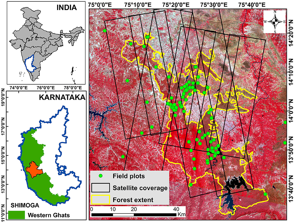
Figure 1. The Shimoga Forest site situated in the Western Ghats region with the location of field plots (green circles). The yellow colored boundary shows the extent of forest in the study area. Multiple baseline TanDEM-X acquisitions over Shimoga Forest are represented as black boxes. The extent is overlaid on a Landsat-8 False Color Composite (FCC) image of Shimoga.

2.2. Field measurement data

Fieldwork was carried out in the Shimoga Forest in March 2019. Field inventory data was collected for 103 sample plots of 31.6 × 31.6 m (0.1 ha). The field plots were established across the Shimoga Forest site. However, inaccessible forests and wildlife movement restricted the choice of forest plot locations. Height (H₁₀), GBH (girth at breast height) and species names were recorded in each plot. The coordinates of the center of each plot were recorded using a Trimble hand-held dual-frequency GPS. The height of each tree was measured using a Criterion RD 1000 Dendrometer (Paragon Instrumentation Engineers Pvt. Ltd, India) along with a Leica Disto D2 Laser Distance Meter (Lecia Camera AG, Germany). H₁₀ is measured considering the 10 highest trees per hectare (Treuhaft and Siqueira, 2000; Khati et al., 2017). The height of the forest plot ranged between 6 and 30.4 m with a mean and SD of 18.2 m and 6 m, respectively. GBH was recorded for 57 out of 103 plots and the mean above-ground biomass (AGB) value was calculated to be 140 t/ha (tons per hectare). A minimum AGB value of 22 t/ha was obtained with a field height of 11.8 m and the highest AGB value of 320 t / ha with a field height of 22.2 m. Species identification was carried out with the technical support of the Karnataka State Forest Department. Most of the plots lie in the deciduous belt and spreads randomly over the forest extent (refer to Figure 1). The H₁₀ height measured for each plot is used as the reference height in the process of height estimation from PolInSAR. Photos taken during the field survey are shown in Figure 2.

FIGURE 2

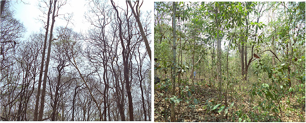
Figure 2. Shimoga Forest field survey photos depicting different forest types: Dry deciduous forest (left) and Semi evergreen forest (right).

As mentioned in Section 2.1, our area of interest for this study is a natural forest and comprises 5 distinct forest types. This is clearly depicted in the photos taken during the field survey. Figure 2 show both the dry deciduous forest range that is completely devoid of leaves during the survey period and the semi-evergreen belt of the Shimoga Forest with leafy plantations. This heterogeneity of the forest is the challenge and motivation behind the PolInSAR height inversion analysis carried out in this article.

2.3. TanDEM-X data acquisitions

The TanDEM-X (TerraSAR-X add-on for Digital Elevation Measurements) mission (Krieger et al., 2007) consists of two X-band radar satellites, viz. TanDEM-X (TDM) and TerraSAR-X (TSX) flying in close orbit configuration. In bistatic mode, either TDM or TSX acts as the transmitter while both the satellites receive the backscattered signal. This simultaneously acquired TDM/TSX pair constitutes a single baseline PolInSAR data set with zero temporal gaps. To evaluate and analyze the potential of TanDEM-X data for forest height inversion in tropical forests in the Western Ghats, 19 fully polarimetric CoSSC (Co-registered Single-Look Slant-range Complex) TerraSAR-X/TanDEM-X pairs with spatial baseline varying between 135 and 302 m acquired during November 2015–February 2016 were utilized (Refer to Figure 1) for the study. The TerraSAR-X/TanDEM-X pair is referred to as TDX throughout the text. The acquisition details of the TDX data sets are summarized in Table 1, where k_z is the vertical wavenumber and the height of ambiguity is the height associated with a phase change 2π, which is further explained in Section 3.3. The 19 acquisitions are numbered in increasing order of height of ambiguity. Each acquisition is then referred to as ACQ-N (N be the corresponding acquisition number as in Table 1) throughout the text. The data sets were collected in bistatic strip map mode at different mean incident angles (20.7–43.2°). The interferometric vertical wavenumber of the datasets ranges from 0.05 to 0.12 rad/m (height of ambiguity: 50.7–114.5 m).

TABLE 1

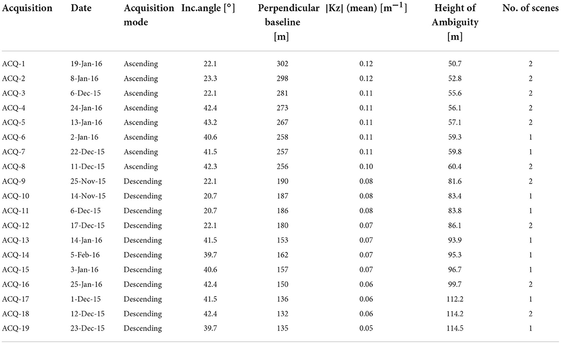
Table 1. Details of TanDEM-X acquisitions in increasing order of Height of Ambiguity.

As mentioned in Section 1, precipitation studies are essential in the forest regions of the Western Ghats, as they are characterized by extensive rainfall throughout the year. Therefore, the precipitation information of the Shimoga Forest has been included here, which will be used for the analysis in Section 4.2. Table 2 shows the precipitation details of all acquisitions, recorded at the Shimoga airport within the test site (near the border of the Shimoga Forest extent). The precipitation data are available from 0 to 12 h before the acquisition by cumulatively adding the values recorded every 3 h. High precipitation values are observed for ACQ-1, ACQ-9, ACQ-17, and ACQ-18, and a significant effect of rainfall is expected in these datasets (discussed in Section 4.2). However, precipitation is negligible (0 or less than 0.5 mm) in the case of other acquisitions.

TABLE 2

Table 2. Cumulative rainfall data of all PolInSAR pairs before acquisition.

Figure 3 shows the available TDX baselines over Shimoga. The acquisitions together cover 95 of 103 field plots. This particular choice of baselines (different vertical wavenumbers) in ascending and descending modes is aimed at achieving an accurate height retrieval over a wide range of tree heights and forest stand densities.

FIGURE 3

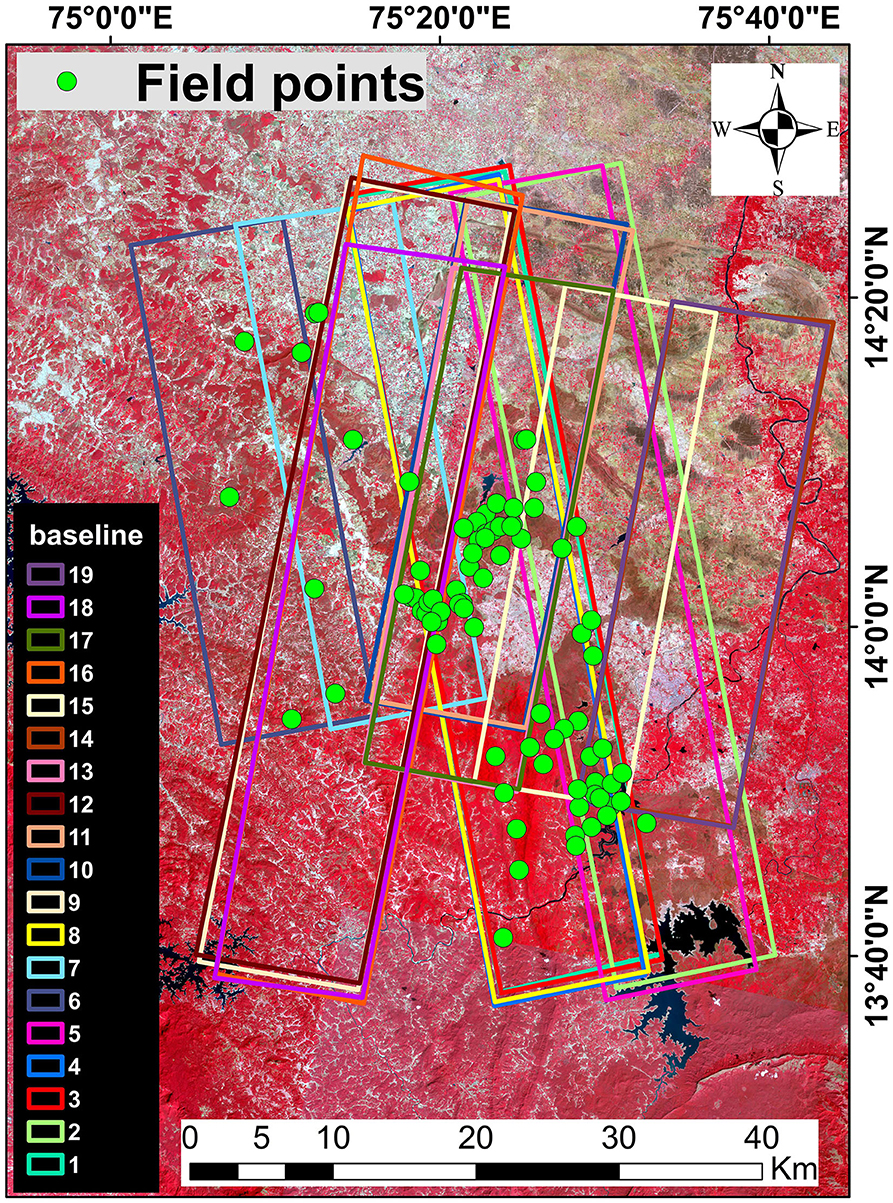
Figure 3. All TanDEM-X acquisitions over the test site with the location of field validation plots. Distinct colors are given to differentiate the 19 baselines. The base image used is a Landsat-8 False Color Composite (FCC) image of Shimoga.

3. Methodology

3.1. Pre-processing

Scattering information of a target pixel as observed by TanDEM-X (TDM) and TerraSAR-X (TSX) is provided by the two SLC images S₁ and S₂ (master and slave) obtained during each PolInSAR acquisition. Scattering matrices [S₁] and [S₂] are generated for master and slave images, which contain backscatter information from different polarization states. Since the acquisitions are fully polarimetric, the backscatter signal in four polarizations indicated as S_XX (XX is the polarization—HH, HV, or VV) constitutes the 2 × 2 (2D) scattering matrix. For every PolInSAR pair, the choice of master and slave images is decided according to the information in the metadata. Here, the PolInSAR pairs are CoSSC products that are already co-registered with each other. Hence, a separate co-registration procedure for slave SLCs to make them comparable to respective master SLCs should be avoided. All the slave SLC data sets are flattened using the synthetic phase fringes derived from TanDEM-X geometry and TanDEM-X DEM. Furthermore, all 19 acquisitions should be resampled at a resolution of 30 m to match the scale of field observations (31.6 × 31.6 m). Resampling to desired resolution was employed by multi-looking at each 2D scattering matrix with azimuth and range look factors calculated by considering a 30 × 30 square pixel of its respective Master SLC. In order to acquire scattering information from multiple targets within a pixel, a 6 × 6 complex coherence matrix [T₆] is derived from the scattering matrix using Pauli basis scattering vectors (Cloude and Papathanassiou, 1998). Complex coherences are calculated for linear (HH, HV, VV), Pauli (HH+VV, HH-VV, HV+VH), and circular (LL, LR, RR), and optimal basis in different polarization states. Because the flat-earth phase has already been eliminated, the resultant interferometric phase relates only to the forest height.

3.2. PolInSAR coherence

A single-baseline polarimetric interferometric SAR system measures each pixel of a scene from two slightly different look angles separated by a normal baseline, resulting in two single-look complex (SLC) images S₁ and S₂. A bistatic, fully polarimetric PolInSAR acquisition is characterized by a 6 × 6 coherency matrix [T₆] (Cloude and Papathanassiou, 2003) shown in Equation (1).

$\begin{array}{l}[T_6]=\langle k.k^{*T}\rangle =\left[\begin{array}{cc}{T}_{11}& {\Omega }_{12}\\ {\Omega }_{12}^{*T}& T_{22}\end{array}\right]\\ k=\frac{1}{\sqrt{2}}[\begin{array}{cccc}{S}_{hh}^1+S_{vv}^1& S_{hh}^1-S_{vv}^1& S_{hv}^1+S_{vh}^1& j(S_{hv}^1-S_{vh}^1)\end{array}\\ {\begin{array}{cccc}{S}_{hh}^2+S_{vv}^2& S_{hh}^2-S_{vv}^2& S_{hv}^2+S_{vh}^2& j(S_{hv}^2-S_{vh}^2)\end{array}]}^T& (1)\end{array}$

where k is the 3-D Pauli scattering vector. Superscripts 1 and 2 denote measurements at the two ends of the baseline. T₁₁ and T₂₂ are 3 × 3 Hermitian polarimetric coherency matrices that represent the polarimetric properties of the two PolInSAR acquisitions. Ω₁₂ is a 3 × 3 non Hermitian matrix that contains the information on variations of interferometric coherences and phases for all possible combinations of polarization states.

The complex interferometric coherence is the key observable in the inversion of the PolInSAR parameter, representing both the interferometric correlation coefficient and the interferometric phase. This coherence is calculated by taking the normalized cross-correlation between the two SAR images S₁ and S₂ obtained from the interferometric acquisition. Complex interferometric coherence (Treuhaft et al., 1996; Papathanassiou and Cloude, 2001) of a PolInSAR pair at all possible polarizations assuming the same polarization $\vec{\omega }$ for both images is estimated by Equation (2).

$\begin{array}{ll}\begin{array}{c}\gamma (\vec{\omega })={\displaystyle \frac{\langle s_1(\vec{\omega })s_2^{*}(\vec{\omega })\rangle }{\sqrt{\langle s_1(\vec{\omega })s_1^{*}(\vec{\omega })\rangle \langle s_2(\vec{\omega })s_2^{*}(\vec{\omega })\rangle }}}\hfill \\ ={\displaystyle \frac{\langle {\vec{\omega }}^{†}[{\Omega }_{12}]\vec{\omega }\rangle }{\sqrt{\langle {\vec{\omega }}^{†}[T_{11}]\vec{\omega }\rangle .\langle {\vec{\omega }}^{†}[T_{22}]\vec{\omega }\rangle }}}\hfill \end{array}& (2)\end{array}$

where 〈.〉 denotes the ensemble average. Coherence amplitude $\left|\gamma (\vec{\omega })\right|$ values range from zero to one, where zero represents complete decorrelation and one represents maximum correlation. Coherence phase (argument of $\gamma (\vec{\omega })$) is the phase difference between two images which is termed an interferogram.

3.3. Vertical wavenumber k_z

Vertical wave number k_z (Bamler and Hartl, 1998) plays a crucial role in the inversion of forest height. The accuracy of the inversion process depends on the selection of appropriate wavenumber and is given by Zebker and Goldstein (1986).

$\begin{array}{ll}{k}_z=m\frac{2\pi }{\lambda }\frac{\delta {\theta }_i}{sin{\theta }_i}=m\frac{2\pi }{\lambda }\frac{B_{\perp }}{Rsin{\theta }_i}\hfill & (3)\end{array}$

where θ_i is the local incidence angle, δθ_i is the change in the local incident angle due to the spatial baseline, λ is the wavelength, B_⊥ is the perpendicular baseline, and R is the slant range distance, and m accounts for the mode of acquisition. For monostatic acquisitions, m = 2 whereas for bistatic acquisitions m = 1. As slant range and incident angle vary for each pixel, k_z is calculated pixel wise as it is dependent on both parameters. k_z is basically a scaling factor that relates the interferometric phase to terrain height h_topo and the relationship is given by Equation (4).

$\begin{array}{ll}\begin{array}{c}{h}_{topo}=\frac{{\varphi }_0}{k_z}\hfill \\ HoA=\frac{2\pi }{k_z}=\frac{\lambda }{B_{\perp }}Rsin{\theta }_i\hfill \end{array}\hfill & (4)\end{array}$

Height of Ambiguity (HoA) in Equation (4) is the terrain height that leads to 2π phase change. From Equation (4), it can be said that the spatial baseline is inversely proportional to HoA which determines the height sensitivity of PolInSAR. For forestry applications, HoA should ideally be greater than the maximum tree height for successful estimation.

3.4. Non volumetric decorrelation

As discussed in Section 3.2, coherence is the similarity between two complex SAR acquisitions. Any changes between two SAR images would result in a decorrelation. A detailed analysis of the factors that contribute to decorrelation in the case of TanDEM-X is explained by Krieger et al. (2007). After compensating for system-induced decorrelation contributions and spectral decorrelation in azimuth and range directions (Zebker and Villasenor, 1992; Bamler and Hartl, 1998; Kugler et al., 2015), the observed interferometric coherence is composed of two decorrelation contributions, namely volume decorrelation (γ_Vol) and non volumetric decorrelations γ_Non.Vol. Information on the vertical forest structure is contained in γ_Vol, which reflects the vertical distribution of the scatterers. The main non volumetric decorrelation sources considered here are spatial baseline decorrelation (γ_spatial), temporal decorrelation (γ_temp), and SNR decorrelation (γ_SNR).

In our case, temporal decorrelation (Hajnsek et al., 2009) is considered negligible as single pass bistatic TerraSAR/TanDEM-X with zero temporal baseline is used as PolInSAR pair. Decorrelation due to spatial baseline has to be taken into account, as all 19 datasets are acquired with different baselines and acquisition geometries. According to Zebker and Villasenor (1992), γ_spatial can be easily calculated from the imaging geometry using the equation as follows

$\begin{array}{ll}{\gamma }_{spatial}=1-\frac{2\left|B_{\perp }\right|\Delta Rco{s}^2\theta }{\lambda R}\hfill & (5)\end{array}$

ΔR in Equation (5) is the range resolution. The spatial baseline decorrelation is directly proportional to the perpendicular baseline and becomes zero for the minimum value of B_⊥ which is the critical baseline B_c. For each polarization channel of a TDX pair, SNR-induced decorrelation can be obtained as follows Kugler et al. (2014).

$\begin{array}{ll}\begin{array}{c}\hfill {\gamma }_{SNR}^{Pol}=\frac{1}{\sqrt{(1+\frac{1}{SN{R}_{TSX}^{Pol}})(1+\frac{1}{SN{R}_{TDX}^{Pol}})}}\end{array}\hfill & (6)\end{array}$

The signal-to-noise ratio (SNR) in Equation (6) of a TSX data set for each polarization channel can be calculated using the corresponding noise equivalent sigma zero (NESZ) patterns provided in the metadata and the backscattering coefficient sigma nought (σ₀). The effect of SNR decorrelation is then removed by calibrating the interferometric coherence using the factor ${\gamma }_{SNR}^{Pol}$ (Kugler et al., 2014).

3.5. Height inversion

The Random Volume over Ground (RVoG) model (Cloude and Papathanassiou, 1998) is a widely used inversion model for the estimation of forest parameters using fully polarimetric and interferometric SAR data. This two-layer model assumes the forest canopy as a random volume layer of thickness h_v on the ground located at height z = z₀. The RVoG model relates the complex coherence $\gamma (\vec{\omega })$ with the vertical reflectivity function F(z) (Hagberg et al., 1995; Treuhaft et al., 1996; Cloude, 2006) that represents the vertical distribution of scatters in the random volume and the relationship is given by a Fourier transformation (Roueff et al., 2011).

$\begin{array}{ll}\begin{array}{c}\gamma (\vec{\omega })=e^{i{k}_z{z}_0}\frac{{\int }_0^{h_v}F(z)e^{i{k}_{z}z}dz}{{\int }_0^{h_v}F(z)dz}\hfill \\ =e^{i{\varphi }_0}\frac{\widetilde{{\gamma }_v}+\mu (\vec{\omega })}{1+\mu (\vec{\omega })}\hfill \end{array}\hfill & (7)\end{array}$

Here, k_z is the effective vertical wavenumber described in detail in Section 3.3. ϕ₀ = k_zz₀ is the topographic or ground phase related to the reference height z₀, which helps to estimate the underlying topography (Fu et al., 2017). $\widetilde{{\gamma }_v}$ denotes the volume-only contribution of the observed interferometric coherence caused by the distribution of scatterers in the vertical direction, which is termed volume decorrelation. $\mu (\vec{\omega })$ represents the amplitude ratio of ground-to-volume scattering for a polarization state $\vec{\omega }$ that accounts for attenuation within the volume layer.

$\begin{array}{ll}\mu (\vec{\omega })=\frac{{\mu }_G(\vec{\omega })}{{\mu }_V(\vec{\omega })}exp\left(-\frac{2\sigma h_v}{cos\theta }\right)\hfill & (8)\end{array}$

where μ_V and μ_G denote the volume and ground scattering amplitudes respectively. θ is the mean angle of incidence and σ is the extinction coefficient that depends on the dielectric constant of the forest layer and the density of the scatterers in it. The interferometric coherence $\gamma (\vec{\omega })$ of Equation (7) becomes a polarization-dependent function, depending on the ground-to-volume ratio $\mu (\vec{\omega })$.

For the inversion process, the RVoG model accounts only for volume decorrelation ignoring all other decorrelation contributions (Zebker and Villasenor, 1992) in the observed interferometric coherence. It is essential to compensate for all non volumetric decorrelations (Bamler and Hartl, 1998) since it will be misinterpreted as additional volume decorrelation, which leads to prominent height estimation errors. After compensating for all non volumetric decorrelation contributions as explained in Section 3.4 and neglecting other system based errors, the total decorrelation is assumed to be solely due to the volume effect. This volume decorrelation is inverted to estimate the forest stand height h_v using different parameter estimation techniques (Cloude and Papathanassiou, 2003). The observed complex volumetric coherence predicted by the RVoG model is shown as

$\begin{array}{ll}\widetilde{{\gamma }_v}(h_v,\sigma ,k_z,\theta )=\frac{{\int }_0^{h_v}exp(\frac{2\sigma h_v}{cos\theta })exp(i{k}_{z}z)dz}{{\int }_0^{h_v}exp(\frac{2\sigma h_v}{cos\theta })dz}\hfill & (9)\end{array}$

Equation (7) can be rewritten as follows

$\begin{array}{ll}\begin{array}{c}\gamma (\vec{\omega })=e^{i{\varphi }_0}(\widetilde{{\gamma }_v}+L(\vec{\omega })(1-\widetilde{{\gamma }_v})),0<L(\vec{\omega })<1\hfill \\ L(\vec{\omega })=\frac{\mu (\vec{\omega })}{1+\mu (\vec{\omega })}\hfill \end{array}\hfill & (10)\end{array}$

Equation (10) shows that the complex interference coherence $\widetilde{{\gamma }_v}$ is distributed in a straight line in the complex plane. The representation of the solution of Equation (10) in the unit circle helps to identify the ground only phase. The best-fit straight line inside the unit circle is found using a total least squares line fit. One of the intersection points of the solution line (best fit line) with the complex plane is considered for the estimation of the topographic phase. The coherence associated with the minimum ground contribution is selected as volume-only coherence $\widetilde{{\gamma }_v}$. The intersection of the best-fit line with the unit circle, which is farther from this point, is the ground phase ϕ₀. Using these two coherence channels representing ground and volume scattering phase centers, the ground-to-volume ratio $\mu (\vec{\omega })$ is calculated.

After estimating the ground topographic phase ϕ₀ (Cloude, 2006), the unknowns h_v and σ are obtained using a 2D optimization problem as shown

$\begin{array}{ll}{\displaystyle \underset{h_v,\sigma }{\text{min}}}||\gamma (k_z,{\mu }_{min})exp(-i{\varphi }_0)-\widetilde{{\gamma }_v}(k_z,h_v,\sigma )||\hfill & (11)\end{array}$

This minimization problem matches the observed coherence with the minimum response from the ground (γ(μ_min) exp(−iϕ₀) $=\widetilde{{\gamma }_v}$) to the coherence expected for pure volume scattering. A 2D lookup table of γ_v is used for a range of h_v and σ values computed from Equation (9). The height estimates obtained from Equation (11) are highly insensitive to structure variations, with a residual error of 10% (Cloude and Papathanassiou, 2003; Papathanassiou et al., 2005). A much simpler and robust height inversion algorithm was developed by Cloude (2006), which accounts for the relative insensitivity of coherence to extinction and the inverted forest height is given by

$\begin{array}{ll}{h}_v=\frac{arg(\widetilde{{\gamma }_v}-{\varphi }_0)}{k_z}+ϵ\frac{2sin{c}^{-1}(|\widetilde{{\gamma }_v}|)}{k_z}\hfill & (12)\end{array}$

where h_v is the tree height, γ_v is the volume-only coherence, ϕ₀ is the ground topographic phase, k_z is the interferometric wavenumber, and ϵ is a constant selected such that the error in Equation (12) is minimized. The first component in Equation (12) is the difference between the volumetric coherence phase and topographic phase estimates, while the second component is augmented to correct for the underestimation of height by the first component. According to Cloude (2006), choosing a ϵ value of 0.4 solves both structural variation and extinction in the volume and minimizes the error in Equation (12). Furthermore, to secure around 10% height accuracy, the minimum ground-to-volume scattering ratio in one of the observed polarization channels needs to be less than −10dB (Papathanassiou et al., 2002). The HV channel often satisfies this requirement and hence cross-polarization measurements are very important for reliable height estimation (Treuhaft et al., 1996).

4. Results and discussion

After a series of PolInSAR preprocessing steps that include interferometry, flat earth removal, and multi-looking, the coherence matrix [T₆] (Equation 1) is generated from the scattering matrices of every TDX pair. Complex coherences are calculated from the [T₆] matrix (Equation 2) for all possible polarization bases. Single baseline PolInSAR height inversion was carried out for each TDX pair from the derived complex coherences using the inversion approach explained in Section 3.5. All pre-processing steps in this work were carried out using NASA-JPL's ISCE (The InSAR Scientific Computing Environment) tool, which is the SAR processor for the upcoming NASA-ISRO SAR (NISAR) mission operational InSAR processing. The vertical wavenumber used for the inversion process should be the local wavenumber k_z accounting for the local angle of incidence on sloped terrain. In the TanDEM-X processing with ISCE, a 30 m NASA DEM over the study site is used to estimate the local incidence angle θ_i. This local incidence angle is then used in the calculation of k_z (Equation 4).

The estimated forest stand height of each baseline is validated against the field validation plots. The field data and the last TDX data acquisition were approximately 4 years or growth periods apart. However, proper cross-validation is still possible, as the maximum increase in biomass of a sample plot during this time period was on the order of approximately 3–5 Mg/ha (Khati et al., 2021). This increase in biomass accounts for growth in both the vertical and horizontal directions. Moreover, there exists a very high ecological competition between the inter- and intra-species resources for growth due to high species diversity in the forest under investigation. This phenomenon particularly limits the vertical growth of trees in a short period of time. By considering the above two observations, the vertical growth that occurred over the years between field campaign and satellite data observation can be considered negligible.

Inversion is evaluated considering parameters such as coefficient of determination (r²), Root Mean Square Error (RMSE), and bias. r² and RMSE are the statistical measures used here to check how accurately the inversion model has estimated the tree heights with reference to field heights. The value of r² is always between 0 (no correlation) and 1 (strong correlation), while lower values of RMSE indicate a better inversion. Bias is the mean of errors calculated by subtracting the estimated height from the respective field height. The validation details of the estimated heights are tabulated in Table 3. For ease of analysis, baselines with the same orbit pass covering the same area of acquisition are categorized into a common group. Hence, the acquisitions are divided into 8 distinct groups (Refer to Table 3).

TABLE 3

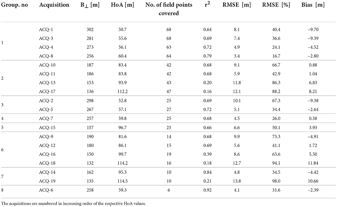
Table 3. Validation of PolInSAR estimated heights of all TDX datasets.

The correlation (r²) between the estimated tree height and the tree height recovered from the field range from 0.16 to 0.92 and the RMSE varies from 3.3 to 13.8 m. Using an HoA range of 50.7 to 114.5 m, r² is observed to increase with HoA to a maximum of 0.92 at 59.3 m and then decrease with increasing HoA. Theoretically, the acquisition having the highest r² (here ACQ-6) should have the strongest correlation with the field data and have the most stable height inversion. However, ACQ-6 having HoA = 59.3 m covers only 6 field points. Correlation analysis of data sets with so few validation points is not reliable. Hence, acquisitions covering less than 20 field plots were omitted in this overall analysis. ACQ-8 with HoA = 60.4 m (point with dotted lines drawn to the axes in Figure 4A) having an r² value of 0.79 is considered to have the strongest correlation as the correlation is calculated from 63 validation plots. Furthermore, the RMSE value decreases with HoA up to 60.4 m (point with dotted lines drawn to axes in Figure 4B and increases with a further increase in HoA. Again, ACQ-8 with HoA 60.4 m exhibits better height inversion with respect to RMSE values (lowest RMSE of 3.4 m).

FIGURE 4

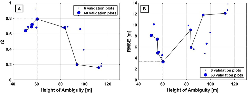
Figure 4. Plot of inversion accuracy parameters against Height of Ambiguity. The size of the circles in the scatter plots are varied with respect to the number of validation plots covered by the particular acquisition. The smallest circle represents acquisition with 6 validations points and the largest circle denotes acquisition with 68 validations points. RMSE and r² of datasets with significant number of validation points are considered in order to see the trend. (A) RMSE Vs HoA. The point with dotted lines drawn to the axis denotes the optimum height that leads to least (best) RMSE. (B) r² Vs Height of ambiguity. The point with dotted lines drawn to the axes represents the optimum height that leads to highest (best) r².

Upon analyzing (Figure 4), it can be inferred that ACQ-8 exhibits the best height inversion in terms of r² and RMSE. However, the inversion accuracy should be analyzed in relation to the vertical wavenumber of the baselines. As mentioned in Section 3.3, k_z scales interferometric phase and coherence to forest height. Since the height inversion process depends on coherence, k_z has a significant impact on its accuracy. A single k_z can result in accurate inversion for only a limited range of forest heights. Large values of k_z (low HoA) would result in under estimation of tall forest stands, as the sensitivity of the coherence to forest height gets saturated at a specific height. Moreover, for too small k_z, even a very low residual non volumetric decorrelation can lead to overestimation of short trees due to unfavorable coherence to height scaling (Kugler et al., 2015). An inappropriate vertical wavenumber for a forest height can lead to an ill-conditioned inversion problem and hence the choice of vertical wavenumber should be such that it optimizes the inversion procedure.

With regard to robust analysis, acquisitions of Group-1 namely ACQ-1, ACQ-3, ACQ-4, and ACQ-8 in ascending mode with 63 common field validation points are considered for further analysis. These acquisitions are chosen because they incorporate a larger area of the study area. Moreover, they cover the maximum number of field plots among all TDX data sets, and hence their correlation with field data is more reliable for validation analysis. From Table 3, it is observed that r² and RMSE of acquisitions in Group-1 improve with an increase in HoA as expected. ACQ-1 with HoA = 50.7 m (k_z = 0.12 rad/m) is least accurate, whereas ACQ-8 with HoA = 60.4 m (k_z = 0.10 rad/m) has the best inversion accuracy among the four acquisitions. Regression analysis in Figure 5 also shows that ACQ-8 is well correlated with field measurement data. Furthermore, height estimation errors of these acquisitions at different height ranges were also taken into account.

FIGURE 5

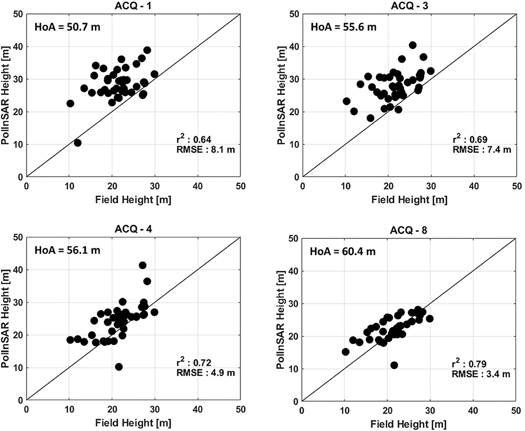
Figure 5. Scatter plot describing the correlation between TDX interferometric height and reference height for validation. The correlation of height estimates with field retrieved height improves substantially with an increase in height of ambiguity.

Table 4 shows the error analysis details of Group-1 acquisitions at different ranges of field heights. The estimation error decreases with an increasing field height range, regardless of the spatial baseline and HoA. Also, estimation error gradually reduces with increasing HoA of baselines, as expected. Here, ACQ-8 has the least estimation error for all field height ranges. Therefore, ACQ-8 acquired on 11 December 2015 exhibits a better correlation with field measurements among Group-1 despite selecting the same validation points for comparison. As discussed earlier, only an optimum value of k_z would result in better inversion for all forest heights. This analysis suggests that since ACQ-8 gives the best correlation results (RMSE = 3.4 m, r² = 0.79, the least estimation error for all field height ranges) in all aspects, its corresponding k_z = 0.10 rad/m can be considered as the optimal wavenumber for this particular study.

TABLE 4

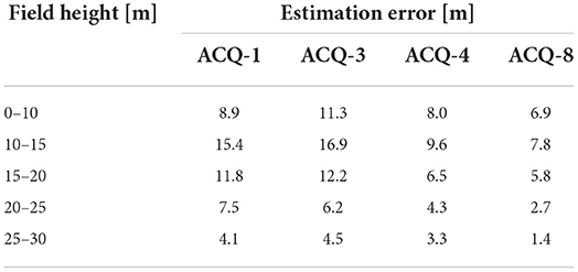
Table 4. Comparison of estimation error for different field height ranges for acquisitions 1, 3, 4, and 8.

Furthermore, the ideal value of HoA should be approximately two times the maximum height of the tree in the given area (Chen et al., 2016; Olesk et al., 2016). In our study, the tallest tree height from field data is 30.4 m which gives the ideal HoA value as 60.8 m and the acceptable value for k_z as 0.10 rad/m. This again confirms the optimum k_z of ACQ-8. As the datasets were not operationally procured exclusively for this study, datasets having HoA between 60 m and 80 m are not available for inversion. However, the absence of datasets in this HoA range will not hinder our analysis. As the optimum HoA for our study is calculated to be 60 m, any acquisition having HoA > 60 m would have k_z < 0.10 rad/m. These smaller values of k_z would lead to overestimation of shorter heights and degrade the height inversion performance. As a result, the baselines with HoA between 60 m and 80 m would have followed the trend in Figure 4.

Figure 6 shows the height map of ACQ-8 obtained after geocoding the height estimates generated by the PolInSAR height inversion process. The obtained PolInSAR forest height map ranging approximately from 0 m to 35 m is overlaid on the LANDSAT-8 optical image for reference. Similar height maps with different height estimates can also be generated for other acquisitions. Geocoded height maps of different acquisitions can be used for large-scale regional and global forest mapping.

FIGURE 6

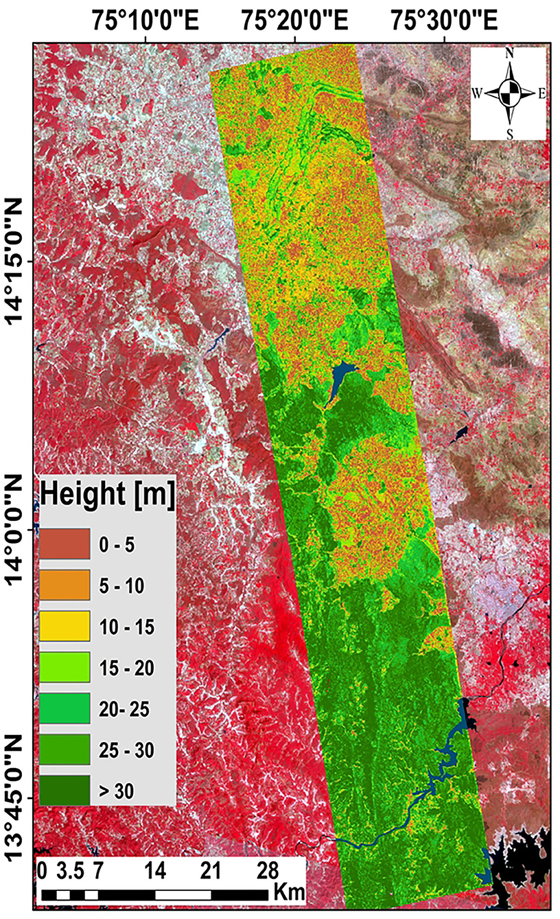
Figure 6. Height Map for 11 December 2015 acquisition obtained after PolInSAR Inversion overlaid on Landsat 8 image. The color-bar indicates the variation in height.

4.1. Influence of incident angle

In this section, the variation in the accuracy of the baselines is investigated based on the influence of the angle of incidence on height inversion (Henderson and Lewis, 1998). As mentioned at the beginning of Section 4, the inversion height estimates of the Group-1 acquisitions exhibited reliable correlation results among other acquisitions. Therefore, acquisitions ACQ-1, ACQ-3, ACQ-4, and ACQ-8 are investigated for this particular analysis. Although they have the same k_z and HoA, ACQ-3, and ACQ-4 exhibit different RMSE values while validating PolInSAR inverted heights against field measured heights (Refer to Table 3). It has to be noted that the RMSE of ACQ-1 (8.1 m) degrades by a factor greater than 2 compared to that of ACQ-8 (3.4 m) even with a spatial baseline variation of 45 m and HoA difference of 10 m between the two acquisitions. This can be addressed by assessing the impact of the incidence angle of acquisitions, as the incident angle is the only parameter varying significantly in this case. Having a shorter wavelength, the X band interacts predominantly with the canopy cover of the forest stand. The change in the angle of incidence results in a varied relative backscatter contribution of the vegetation canopy elements (Tighe et al., 2012). At a steep angle of incidence (small θ), the radar penetrates the canopy, leading to greater exposure to the lower portion of the forest cover. Therefore, signal interactions with the trunks are significantly higher compared to those of the tree crown region. However, these interactions in the lower vegetation layer are mostly attenuated and shadowed by the upper canopy on their way back to the radar. At the same time, a major contribution of backscatter at shallow incident angles (large θ) is provided by the high relative volume scattering from the upper canopy.

In ACQ-1 and ACQ-3 with θ = 22.1° (steep incidence), penetration inside the canopy results in an incorrect estimation of the phase center height, which degrades the accuracy of the inversion. While in ACQ-4 and ACQ-8, phase center height lies along the upper canopy due to large volume scattering from the canopy envelope, leading to more accurate estimates of the height of the vegetation canopy in shallow incidence (θ = 42.4°). Furthermore, the mean complex coherences of ACQ-3 and ACQ-4 for a 10 × 10 pixel window over the forest region were investigated. Coherence circles in Figure 7 geometrically show the effect of incidence angle on height inversion. As mentioned earlier, Equation (10) depicts interferometric coherence as a straight line inside the complex plane by varying μ values. For accurate inversion using the RVoG model, the complex coherences should fit in a line segment (Papathanassiou and Cloude, 2001). Forest scatterers in ACQ-4 (Figure 7A) exhibit good linearity in the complex plane. This indicates accurate RVoG inversion in ACQ-4 and subsequently supports improved height estimation compared to ACQ-3 for which coherences are not well distributed on the complex circle (Figure 7B). The regression analysis depicted in Figure 5 also shows a high correlation between the estimated heights and the field heights in ACQ-8 compared to ACQ-1. However, the differences in k_z and HoA resulted in a slight difference in accuracy between ACQ-1 and ACQ-3 even with the same incident angle. The same explanation holds for the slight increase in the RMSE of ACQ-8 compared to ACQ-4.

FIGURE 7

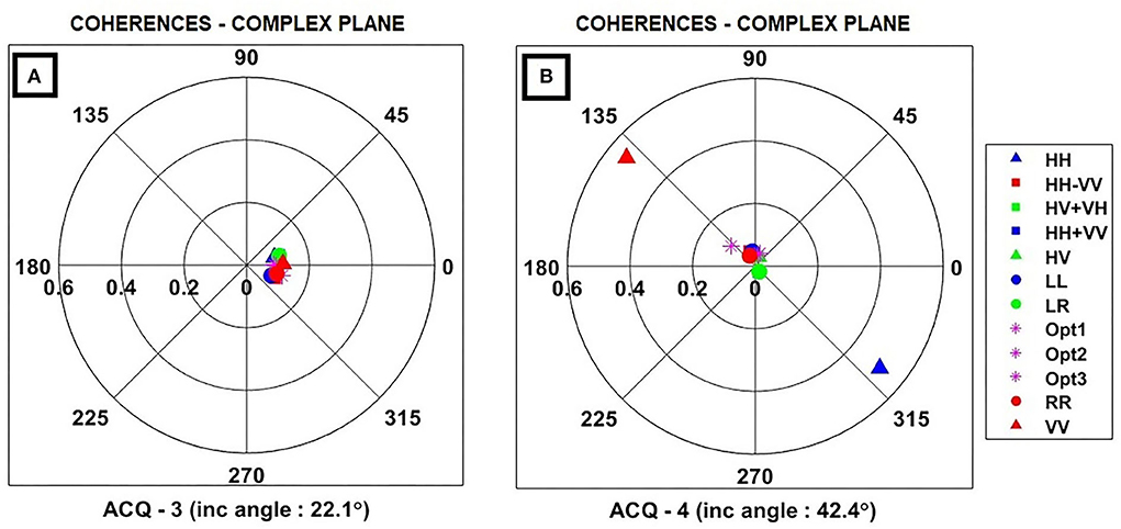
Figure 7. Complex coherences plotted for linear, Pauli, circular, and optimal basis. Color code opted: Blue - HH, HH+VV, LL; Green - HV, HV+VH, LR; Red - VV, HH-VV, RR; Magenta - optimal basis. (A) Complex plane signature of ACQ-3 having steep angle of incidence. (B) Complex plane signature of ACQ-4 having shallow angle of incidence.

4.2. Effect of rainfall

As already mentioned in Section 1 and Section 2.3, the impact of rainfall in the Shimoga Forest region is worth analyzing, as it is characterized by intermittent precipitation throughout the year. Furthermore, surface moisture in vegetation resulting from rainfall can alter the backscatter contributions from the vegetation canopy and the ground surface (Henderson and Lewis, 1998). Changes in the dielectric properties of the canopy due to the presence of moisture have a significant impact on the observed PolInSAR coherences and can inhibit the canopy height estimation. Looking into the validation results, it was interesting to note that there is a significant difference in the RMSE values between ACQ-9 and ACQ-12 despite having a similar spatial baseline (≈190) and HoA (≈85). ACQ-9 has an RMSE of 9.9 m while the RMSE of ACQ-12 is 5.6 m. Since the datasets are acquired with less than a 1-month temporal gap, there is no chance of seasonal change impact on estimation. From the rainfall details, it is observed that there was a cumulative rainfall of 1.8 mm on 25 November 2015 (acquisition date of ACQ-9) while no rainfall was recorded on the date of acquisition of ACQ-12. In this case, the coherence regions of the acquisitions were also investigated and the mean coherence across a 10 x 10 sample window within the forest region was computed. The mean coherence of ACQ-9 and ACQ-12 was found to be 0.18 and 0.55, respectively. The low correlations of ACQ-9 compared to ACQ-12 in the forest can be attributed to the presence of water particles on the canopy surface.

Apart from the coherence magnitude, the coherence phase can also be considered to justify the degradation of accuracy during rain. It is known that the coherence region is defined by the loci of the interferometric coherences on the complex circle for all possible polarizations. The angular extent of the coherence region depicts the variance of the interferometric phase center as a function of polarization (Kugler et al., 2014). The maximum angular difference Δϕ corresponds to the maximum variance of the interferometric phase center for different polarizations. Δϕ is scaled with the vertical wavenumber to obtain the maximum height difference (phase center height) Δh. In the case of ACQ-9 with rainfall (Figure 8A), the coherences have a larger angular separation compared to the coherences inside the complex circle of ACQ-12 (Figure 8B). Δϕ for ACQ-9 is greater than that for ACQ-12. Since Δϕ and Δh are directly related, the phase center height calculated by PolInSAR would be much higher than that of ACQ-12. This could have led to an overestimation of the ACQ-9 dataset acquired during rainfall and resulted in a high RMSE compared to ACQ-12. Even though high precipitation values are observed for ACQ-17 and ACQ-18, acquisitions with no rainfall in the same region are not available for comparison. Therefore, the effect of rainfall on the PolInSAR estimates of these acquisitions could not be analyzed.

FIGURE 8

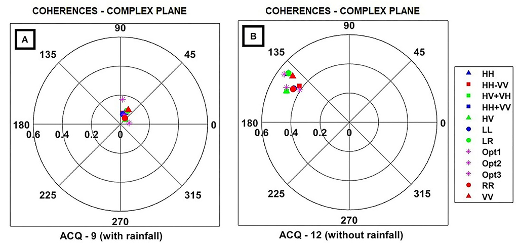
Figure 8. Polarimetric variation of interferometric coherence. Complex coherences are plotted for linear, Pauli, circular, and optimal basis. Color code opted: Blue - HH, HH+VV, LL; Green - HV, HV+VH, LR; Red - VV, HH-VV, RR; Magenta - optimal basis. (A) Complex plane signature of ACQ-9 (with rainfall). (B) Complex plane signature of ACQ-12 (without rainfall).

4.3. Forest biomass impact on height inversion

Above ground biomass (AGB) is calculated for 57 plots out of the total 103 field validation plots. Figure 9 plots the variability of PolInSAR derived height estimation error of acquisitions 1, 8, and 11 with AGB values. The tree density in the AGB plots covered by the available baselines ranged between 40 and 220 individuals per hectare. The error in height estimates decreases with increasing forest stand density for all baselines irrespective of the Height of Ambiguity, spatial baseline, and incidence angle. Comparing HoA = 50.7 m and HoA = 83.8 m shows a lower estimation error for low forest densities, while a slightly higher error at large AGB values. The baseline with HoA = 60.4 m shows the least estimation error of 2 m for highly dense forest stands among all baselines.

FIGURE 9

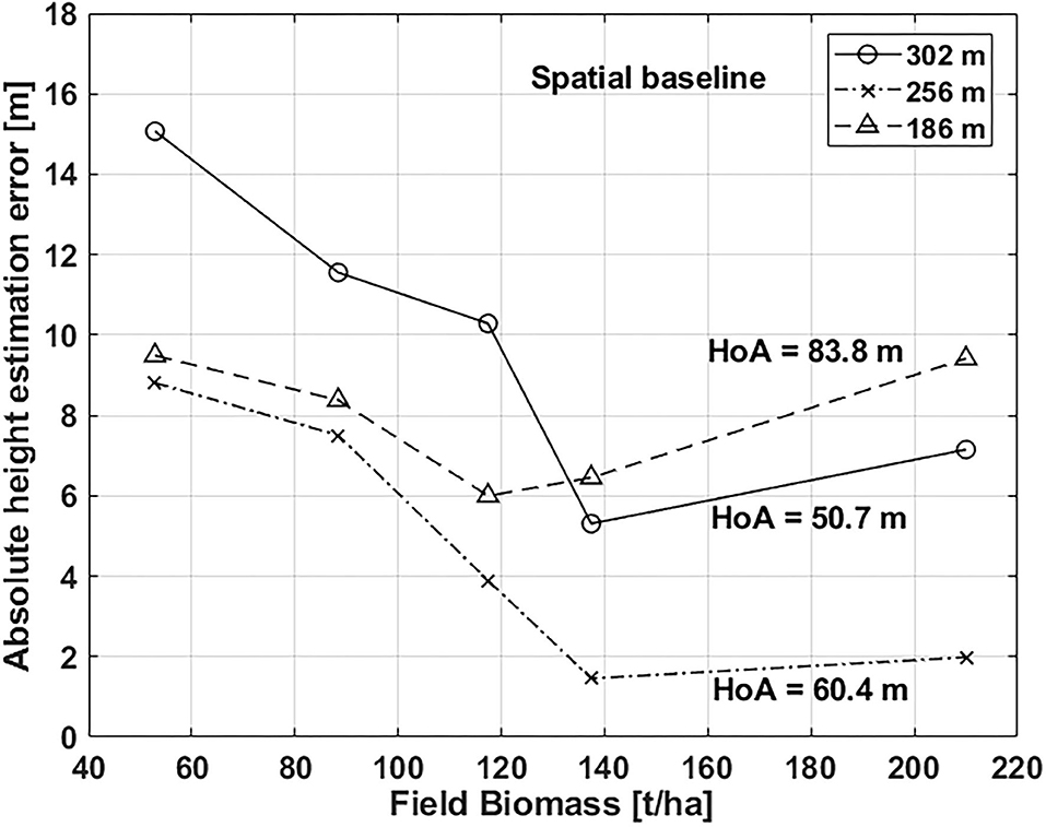
Figure 9. Variation of PolInSAR estimated height error with field-estimated forest biomass. Error in estimated heights decreases significantly with an increase in field AGB values. Height estimation error shows similar trend with biomass for acquisitions with different spatial baselines.

In general, the estimation error decreases linearly with the increase in biomass from 40 t/ha to 140 t/ha. RVoG height inversion is based on the assumption that there is no ground component for at least one of the observed polarization channels (μ_min = 0) (Kugler et al., 2015). The presence of surface components in $\widetilde{{\gamma }_v}$ results in nonzero μ values that lead to an inaccurate height inversion (Cloude, 2006). Hence, Equation (12) probably did not provide a unique height solution for AGB plots with relatively sparse forest stands (40–140 t/ha) which led to a high estimation error. The error appears to be almost consistent for forest stands with AGB values ranging from 150 to 220 t/ha in the three baselines considered for comparison. The presence of a dense canopy in these plots resulted in high volume scattering from the canopy, which in turn resulted in an accurate height estimate. Similar trends were also observed by Khati et al. (2018) for various multi-frequency satellite acquisitions, including TanDEM-X.

4.4. The potential of a merged height approach

Figure 3 shows that the acquired baselines cover different parts of the forest, so combining the heights retrieved from these multiple baselines should give a larger picture of the study area. To effectively combine the inversion results of various baselines, individual height maps were first geocoded in latitude and longitude at a resolution of 12 m. Height inversions that have too small values of k_z (<0.06) and baselines that cover field points less than 20 were excluded from the combined height map generation. Height maps of data sets that exhibited good correlation with field data were superimposed to obtain a consolidated height map of the entire study area. This consolidated height map was masked by our desired forest extent, which removed the unwanted urban area estimates from the height map. Averaging of heights was employed at lat/lon locations where height estimates from two or more acquisitions were available. Figure 10 shows the inverted heights of the selected baselines with maximum accuracy. This map provides canopy height estimates over a wider region of the Shimoga Forest. The same procedure can be adapted to generate global/regional forest maps.

FIGURE 10

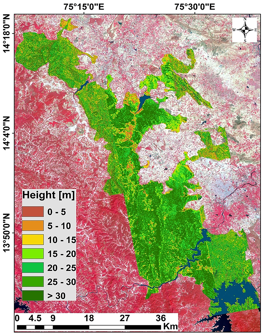
Figure 10. Map of PolInSAR extracted heights over the Shimoga Forest extend. This map shows the mosaic of canopy heights of selected baselines overlaid on the Sentinel-2 optical image. Here, height maps of acquisitions that display good inversion accuracy are mosaicked together and masked by the desired forest extent.

It is clear from the discussion so far that several factors influence the prediction of tree heights. The single baseline inversion results of the 19 acquisitions have demonstrated an unstable correlation coefficient (r² : 0.16–0.92) and variable RMSE (3.3–13.8 m), depending on the choice of the vertical wavenumber, spatial baseline, and the number of field samples covered. Although ACQ-8 has better correlation results among all acquisitions, none of the single baseline results could provide an excellent forest height estimate for the entire height range between 6 and 30.4 m. Each baseline provides a solution space at a certain height value. Therefore, instead of combining all the height maps of the selected baselines, an improved height accuracy can be achieved by appropriately selecting only the best height estimates from the available baselines. Several multibaseline inversion approaches (Neumann et al., 2010; Lee et al., 2011, 2018; Pourshamsi et al., 2018) have been developed earlier in this regard, where the prior knowledge on forest height or machine learning approach is utilized to select good height estimates among multiple baselines.

In this section, a simpler way of merging optimum heights from multiple baselines is adapted and its influence on inversion accuracy is investigated. It is known that each acquisition provides different height estimates for a given field location. Hence, all available baselines are merged by manually selecting the optimum height for each field plot. PolInSAR height estimate that has a minimum absolute difference with the H₁₀ value is chosen as the optimum height (h_opt) for a given field plot. The resultant optimum height is validated against the field height to evaluate the accuracy (Refer to Figure 11). The error bars in Figure 11 represent the range of values h_opt can occupy for a given H₁₀. This deviation for each h_opt is calculated by taking the SD of the 19 PolInSAR estimation errors. The best heights selected for each plot together exhibit a very high acorrelation with field data having a correlation coefficient of 0.92 and an RMSE of 1.9 m. This approach shows that there is at least one height estimate among the 19 PolInSAR heights, which is very close to H₁₀, and that the combined height of multiple baselines yields the best regression results compared to any other single baseline height estimate. This merged height approach with multiple baselines is extremely beneficial in the study of forests with wide height ranges, especially natural forests.

FIGURE 11

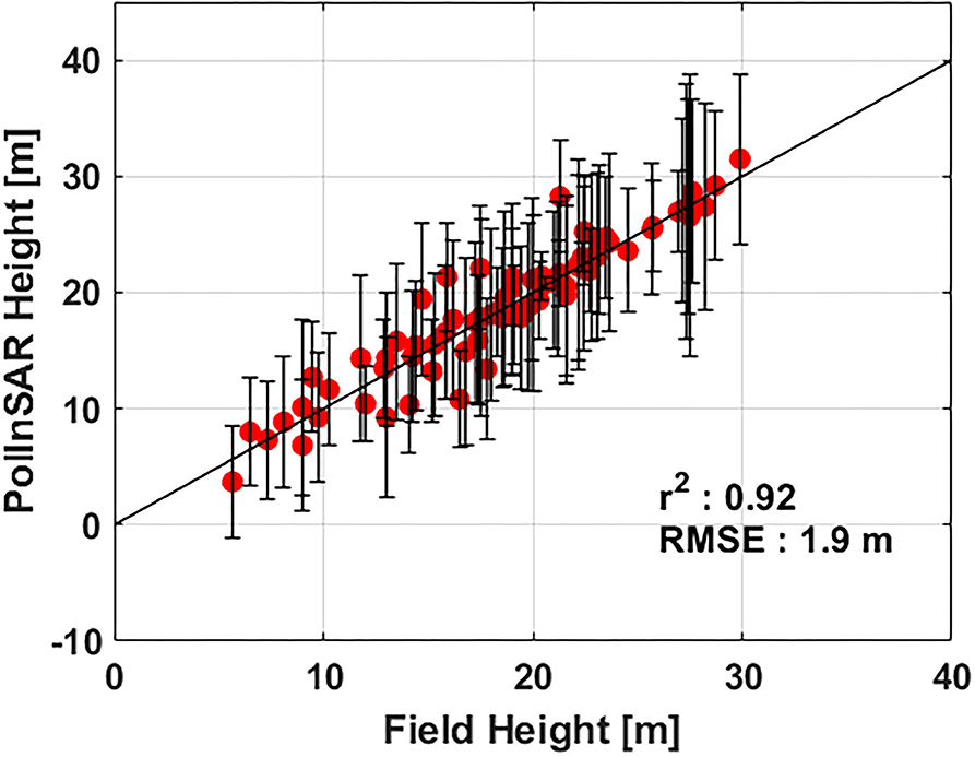
Figure 11. Validation of optimum height vs. field height. The vertical error bars represent ±σ confidence interval of estimates.

5. Conclusion

This article evaluates the potential of TanDEM-X data for estimating PolInSAR height in a heterogeneous tropical forest in Shimoga Forest, Western Ghats, India. The single-baseline PolInSAR height inversion was implemented using the modified RVoG model. Forest height inversion performance of multiple baselines has been assessed. The data are acquired over a mature, fairly dense tropical forest in the Western Ghats with plot heights ranging from 6 m to 30.4 m and AGB values varying from 22 t/ha to 320 t/ha. In the field campaign, very few forest locations had plot heights less than 10 m, which could limit the ability of this study to fully characterize the accuracy of height inversion for low-height forest regions. Non-operational procurement of datasets has led to the non-availability of acquisitions with a wide range of baselines. Therefore, acquisitions with HoA ranging from 60 m to 80 m were not available for the height inversion study.

Single baseline inversion results have demonstrated a range of correlation coefficients (r² : 0.16–0.92) and variable RMSE (3.3–13.8 m). Overall, the PolInSAR height estimates of the acquired datasets are well correlated with the reference field heights. Reliable regression results of acquisitions covering sufficient field points (here 20) are only considered for validation. The RMSE of acquisitions increases with the Height of Ambiguity up to a height of 60.4 m and decreases with a further increase of HoA. At the same time, r² decreases with increasing HoA up to 60.4 m and increases after that. This optimum height of 60.4 m is possessed by the data set acquired on 11 December 2015 (ACQ-8) covering 68 validation points. Validation results of ACQ-8 indicate high accuracy, with RMSE = 3.4 m and r² = 0.79. The trends observed for r² and RMSE are due to the effect of varying the spatial baseline and the vertical wavenumber k_z. Only a limited range of tree heights can be inverted accurately using a particular k_z. Large values of k_z lead to the underestimation of larger heights, whereas small k_z values result in overestimation. The results also confirm the role of optimal wavenumber on the accuracy of PolInSAR height inversion. The optimal wavenumber for our study is observed for ACQ-8 with k_z : 0.1 rad/m.

In addition to vertical wavenumber, the influence of parameters such as incident angle, precipitation, and field biomass on height retrieval is also discussed. ACQ-1 and ACQ-8 having a similar baseline, acquired with only a few days of temporal gaps (same season), are expected to have similar PolInSAR regression results. Instead, ACQ-1 exhibits an RMSE of 8.1 m which is approximately 2.4 times the RMSE of ACQ-8. This degradation in the accuracy of ACQ-1 is due to its steep incident angle acquisition. At steep incidence angles, phase center height is wrongly estimated due to high penetration inside the canopy. Due to the shallow angle of incidence in ACQ-8, the volumetric phase center is shifted up to match the actual canopy height, which leads to an accurate estimation of height. Furthermore, it is observed that rainfall leads to canopy backscatter variations, that affect the PolInSAR inversion. ACQ-12 having the same spatial baseline and HoA as ACQ-9 provides highly accurate height estimates compared to the latter. Both data sets were acquired in the same season with the same angle of incidence. Precipitation of 1.8 mm was observed on the date of acquisition of ACQ-9 and resulted in an overestimation of lower heights with RMSE = 9.9 m, which is explained in detail in Section 4.2. At the same time, ACQ-12 with zero rainfall recorded had an RMSE of 5.6 m. This shows that the PolInSAR inversion is affected by rainfall, which decreases the inversion accuracy. Even though a good height inversion is observed over both high AGB and low AGB forests, overall there is an inverse trend between AGB and height estimation error. ACQ-1, ACQ-8, and ACQ-11 with different HoA ranges were analyzed in this regard.

A merged height approach was explored by combining the height estimates of all the baselines that exhibit the least estimation error. Merging the optimum PolInSAR height estimates from multiple baselines improved the result compared to the single-baseline approach. The estimated height from this approach had a higher accuracy with an RMSE = 1.9 m and an r² = 0.92. Previous studies used a priori knowledge of forest height or an automated approach to select the best heights from multiple baselines. The use of such robust techniques, along with the wide range of baselines and validation points, can provide a much more reliable PolInSAR height inversion analysis, which can be adopted for future work. However, as very few height estimation studies were reported over the Western Ghats, this work can be considered as a base for the upcoming PolInSAR studies in this area. To conclude, it can be said that this paper highlights the potential of bistatic TanDEM-X data to successfully estimate heights over natural forests in India and enabled large scale forest height mapping over the Shimoga Forest.

Data availability statement

The data analyzed in this study is subject to the following licenses/restrictions: Satellite data and field data information are restricted due to agreements between the authors and the data providers. Requests to access these datasets should be directed to gulab.singh@iitb.ac.in.

Author contributions

Conceptualization: SR, UK, and GS. Methodology: SR and UK. Data acquisition, supervision, project administration, and infrastructure support: GS. Data curation, processing, writing—original draft preparation, and analysis: SR. Fieldwork collection: MM. Writing—review and editing: UK and GS. Funding acquisition: GS and ST. All authors contributed to the article and approved the submitted version.

Funding

A part of this study was carried out under Indo-Italy S&T Cooperation with project number NT/ITALY/P-1/2016(ER) between IIT Bombay and Politecnico di Milano. The research was partially supported by the Space Application Center, Indian Space Research Organization (ISRO), under the NISAR project coded Eco-05.

Acknowledgments

The authors would like to thank the Forest Department of Karnataka State for technical support during the field campaign.

Conflict of interest

The authors declare that the research was conducted in the absence of any commercial or financial relationships that could be construed as a potential conflict of interest.

Publisher's note

All claims expressed in this article are solely those of the authors and do not necessarily represent those of their affiliated organizations, or those of the publisher, the editors and the reviewers. Any product that may be evaluated in this article, or claim that may be made by its manufacturer, is not guaranteed or endorsed by the publisher.

References

Bamler, R., and Hartl, P. (1998). Synthetic aperture radar interferometry: inverse problems. IEEE Trans. Geosci. Remote Sens. 14, 41–54. doi: 10.1088/0266-5611/14/4/001

CrossRef Full Text

Berninger, A., Lohberger, S., Zhang, D., and Siegert, F. (2019). Canopy height and above-ground biomass retrieval in tropical forests using multi-pass X-and C-band PolInSAR data. Remote Sens. 11, 2105. doi: 10.3390/rs11182105

CrossRef Full Text | Google Scholar

Bhanu Prakash, M., and Kumar, S. (2021). PolInSAR decorrelation-based decomposition modelling of spaceborne multifrequency SAR data. Int. J. Remote Sens. 42, 1398–1419. doi: 10.1080/01431161.2020.1829155

CrossRef Full Text | Google Scholar

Champion, H., and Seth, S. (1968). A Revised Survey of the Forest Types of INDIA. New Delhi: Govt. of India Press.

Google Scholar

Chen, H., Cloude, S. R., and Goodenough, D. G. (2016). Forest canopy height estimation using Tandem-X coherence data. IEEE J. Select. Top. Appl. Earth Observat. Remote Sens. 9, 3177–3188. doi: 10.1109/JSTARS.2016.2582722

PubMed Abstract | CrossRef Full Text | Google Scholar

Cloude, S. (2006). Polarization coherence tomography. Radio Sci. 41, 1–27. doi: 10.1029/2005RS003436

CrossRef Full Text | Google Scholar

Cloude, S. (2010). Polarisation: Applications in Remote Sensing. Oxford: Oxford University Press.

PubMed Abstract | Google Scholar

Cloude, S., and Papathanassiou, K. (2003). Three-stage inversion process for polarimetric SAR interferometry. IEEE Proc. Radar Sonar Navigat. 150, 125–134. doi: 10.1049/ip-rsn:20030449

CrossRef Full Text | Google Scholar

Cloude, S. R., and Papathanassiou, K. P. (1997). “Coherence optimisation in polarimetric SAR interferometry,” in IGARSS'97. 1997 IEEE International Geoscience and Remote Sensing Symposium Proceedings. Remote Sensing-A Scientific Vision for Sustainable Development, Vol. 4 (Singapore: IEEE), 1932–1934.

Google Scholar

Cloude, S. R., and Papathanassiou, K. P. (1998). Polarimetric SAR interferometry. IEEE Trans. Geosci. Remote Sens. 36, 1551–1565. doi: 10.1109/36.718859

CrossRef Full Text | Google Scholar

Feldpausch, T. R., Lloyd, J., Lewis, S. L., Brienen, R. J., Gloor, M., Monteagudo Mendoza, A., et al. (2012). Tree height integrated into pantropical forest biomass estimates. Biogeosciences 9, 3381–3403. doi: 10.5194/bg-9-3381-2012

CrossRef Full Text | Google Scholar

Fu, H., Zhu, J., Wang, C., Wang, H., and Zhao, R. (2017). Underlying topography estimation over forest areas using high resolution P-band single baseline PolInSAR data. Remote Sens. 9, 363. doi: 10.3390/rs9040363

CrossRef Full Text | Google Scholar

Garestier, F., Dubois-Fernandez, P. C., and Champion, I. (2008). Forest height inversion using high-resolution P-band PolInSAR data. IEEE Trans. Geosci. Remote Sens. 46, 3544–3559. doi: 10.1109/TGRS.2008.922032

CrossRef Full Text | Google Scholar

Ghosh, S., and Behera, M. (2017). Forest canopy height estimation using satellite laser altimetry: a case study in the Western Ghats, India. Appl. Geomat. 9, 159–166. doi: 10.1007/s12518-017-0190-2

CrossRef Full Text | Google Scholar

Hagberg, J. O., Ulander, L. M. H., and Askne, J. (1995). Repeat pass SAR interferometry over forested terrain. IEEE Trans. Geosci. Remote Sens. 33, 331–340. doi: 10.1109/TGRS.1995.8746014

CrossRef Full Text | Google Scholar

Hajnsek, I., Kugler, F., Lee, S.-K., and Papathanassiou, K. P. (2009). Tropical forest parameter estimation by means of PolInSAR: the INDREX-II campaign. IEEE Trans. Geosci. Remote Sens. 47, 481–493. doi: 10.1109/TGRS.2008.2009437

CrossRef Full Text | Google Scholar

Harrell, P., Kasischke, E., Bourgeau-Chavez, L., Haney, E., and Christensen, N. (1997). Evaluation of approaches to estimating aboveground biomass in southern pine forests using sir-c data. Remote Sens. Environ. 59, 223–233. doi: 10.1016/S0034-4257(96)00155-1

CrossRef Full Text | Google Scholar

Hemanjali, A., Pramod Kumar, G., Somashekar, R., and Nagaraja, B. (2015). Assessment of forest encroachment in Shimoga district of Western Ghats, India, using remote sensing and GIS. Int. J. Adv. Technol. Eng. Res. 5, 25–30. Available online at: https://data.landportal.info/library/resources/issn-no-2250-3536/assessment-forest-encroachment-shimoga-district-western-ghats

Henderson, F., and Lewis, A. (1998). Principles and Applications of Imaging Radar. Manual of Remote Sensing, Vol. 2, 3rd Edn. Somerset, NJ: John Wiley and Sons.

Google Scholar

Jha, C., Singhal, J., Reddy, C., Rajashekar, G., Maity, S., Patnaik, C., et al. (2019). Characterization of species diversity and forest health using AVIRIS-NG hyperspectral remote sensing data. Curr. Sci. 116, 1135. doi: 10.18520/cs/v116/i7/1124-1135

CrossRef Full Text | Google Scholar

Khati, U., Lavalle, M., Shiroma, G. H., Meyer, V., and Chapman, B. (2020). Assessment of forest biomass estimation from dry and wet SAR acquisitions collected during the 2019 UAVSAR AM-PM campaign in southeastern United States. Remote Sens. 12, 3397. doi: 10.3390/rs12203397

CrossRef Full Text | Google Scholar

Khati, U., Lavalle, M., and Singh, G. (2021). The role of time series L-band SAR and GEDI in mapping sub tropical above ground biomass. Front. Earth Sci. 9, 752254. doi: 10.3389/feart.2021.752254

CrossRef Full Text | Google Scholar

Khati, U., and Singh, G. (2015). “Bistatic PolInSAR for forest height estimation: results from TanDEM-X,” in 2015 IEEE 5th Asia-Pacific Conference on Synthetic Aperture Radar (APSAR) (Singapore: IEEE), 214–217.

Google Scholar

Khati, U., Singh, G., and Ferro-Famil, L. (2017). Analysis of seasonal effects on forest parameter estimation of Indian deciduous forest using TerraSAR-X PolInSAR acquisitions. Remote Sens. Environ. 199, 265–276. doi: 10.1016/j.rse.2017.07.019

CrossRef Full Text | Google Scholar

Khati, U., Singh, G., and Kumar, S. (2018). Potential of spaceborne PolInSAR for forest canopy height estimation over India–A case study using fully polarimetric L-, C-, and X-Band SAR data. IEEE J. Select. Top. Appl. Earth Observat. Remote Sens. 11, 2406–2416. doi: 10.1109/JSTARS.2018.2835388

CrossRef Full Text | Google Scholar

Krieger, G., Moreira, A., Fiedler, H., Hajnsek, I., Werner, M., Younis, M., et al. (2007). TanDEM-X: a satellite formation for high resolution SAR interferometry. IEEE Trans. Geosci. Remote Sens. 45, 3317–3341. doi: 10.1109/TGRS.2007.900693

CrossRef Full Text | Google Scholar

Kugler, F., Koudogbo, F. N., Gutjahr, K., and Papathanassiou, K. P. (2006). “Frequency effects in PolInSAR forest height estimation,” in Proceedings of EUSAR (Dresden), 16–18.

Google Scholar

Kugler, F., Lee, S. K., Hajnsek, I., and Papathanassiou, K. P. (2015). Forest height estimation by means of PolInSAR data inversion: THE role of the vertical wavenumber. IEEE Trans. Geosci. Remote Sens. 53, 5294–5311. doi: 10.1109/TGRS.2015.2420996

CrossRef Full Text | Google Scholar

Kugler, F., Schulze, D., Hajnsek, I., Pretzsch, H., and Papathanassiou, K. P. (2014). TanDEM-X PolInSAR performance for forest height estimation. IEEE Trans. Geosci. Remote Sens. 52, 6404–6422. doi: 10.1109/TGRS.2013.2296533

CrossRef Full Text | Google Scholar

Kumar, S., Garg, R. D., Kushwaha, S., Jayawardhana, W., and Agarwal, S. (2017a). Bistatic PolInSAR inversion modelling for plant height retrieval in a tropical forest. Proc. Natl. Acad. Sci. India A Phys. Sci. 87, 817–826. doi: 10.1007/s40010-017-0451-9

CrossRef Full Text | Google Scholar

Kumar, S., Govil, H., Srivastava, P. K., Thakur, P. K., and Kushwaha, S. P. (2020). Spaceborne multifrequency PolInSAR based inversion modelling for forest height retrieval. Remote Sens. 12, 4042. doi: 10.3390/rs12244042

CrossRef Full Text | Google Scholar

Kumar, S., Khati, U. G., Chandola, S., Agrawal, S., and Kushwaha, S. P. (2017b). Polarimetric SAR interferometry based modeling for tree height and aboveground biomass retrieval in a tropical deciduous forest. Adv. Space Res. 60, 571–586. doi: 10.1016/j.asr.2017.04.018

CrossRef Full Text | Google Scholar

Kumar, S., Pandey, U., Kushwaha, S. P., Chatterjee, R. S., and Bijker, W. (2012). Aboveground biomass estimation of tropical forest from Envisat advanced synthetic aperture radar data using modeling approach. J. Appl. Remote Sens. 6, 063588. doi: 10.1117/1.JRS.6.063588

CrossRef Full Text | Google Scholar

Lee, S., Kugler, F., Papathanassiou, K., and Hajnsek, I. (2011). “Multibaseline polarimetric SAR interferometry forest height inversion approaches,” in Proceedings of ESA POLinSAR Workshop, Vol. 2 (Frascati).

Google Scholar

Lee, S.-K., Kugler, F., Papathanassiou, K., and Moreira, A. (2009). “Forest height estimation by means of PolInSAR limitations posed by temporal decorrelation,” in Proceedings of 11th ALOS Kyoto Carbon Initiative (Tsukuba: JAXA TKSC), 13–16.

Google Scholar

Lee, S. K., Fatoyinbo, T. E., Lagomasino, D., Feliciano, E., and Trettin, C. (2018). Multibaseline TanDEM-X mangrove height estimation: the selection of the vertical wavenumber. IEEE J. Select. Top. Appl. Earth Observat. Remote Sens. 11, 3434–3442. doi: 10.1109/JSTARS.2018.2835647

CrossRef Full Text | Google Scholar

Lefsky, M. A., Harding, D. J., Keller, M., Cohen, W. B., Carabajal, C. C., Del Bom Espirito-Santo, F., et al. (2005). Estimates of forest canopy height and aboveground biomass using ICESat. Geophys. Res. Lett. 32, 1–4. doi: 10.1029/2005GL023971

PubMed Abstract | CrossRef Full Text | Google Scholar

Liang, S. (2005). Quantitative Remote Sensing of Land Surfaces. Hoboken, NJ: John Wiley & Sons.

Google Scholar

Lima, A. J. N., Suwa, R., de Mello Ribeiro, G. H. P., Kajimoto, T., dos Santos, J., da Silva, R. P., et al. (2012). Allometric models for estimating above-and below-ground biomass in Amazonian forests at S ao Gabriel da Cachoeira in the upper Rio Negro, Brazil. For. Ecol. Manag. 277, 163–172. doi: 10.1016/j.foreco.2012.04.028

CrossRef Full Text | Google Scholar

Lucas, R., Armston, J., Fairfax, R., Fensham, R., Accad, A., Carreiras, J., et al. (2010). An evaluation of the ALOS PALSAR L-band backscatter–Above ground biomass relationship Queensland, Australia: impacts of surface moisture condition and vegetation structure. IEEE J. Select. Top. Appl. Earth Observat. Remote Sens. 3, 576–593. doi: 10.1109/JSTARS.2010.2086436

CrossRef Full Text | Google Scholar

Neumann, M., Ferro-Famil, L., and Reigber, A. (2010). Estimation of forest structure, ground, and canopy layer characteristics from multibaseline polarimetric interferometric SAR data. IEEE Trans. Geosci. Remote Sens. 48(3 Part 1), 1086–1104. doi: 10.1109/TGRS.2009.2031101

CrossRef Full Text | Google Scholar

Olesk, A., Praks, J., Antropov, O., Zalite, K., Arumäe, T., and Voormansik, K. (2016). Interferometric SAR coherence models for characterization of hemiboreal forests using TanDEM-X data. Remote Sens. 8, 700. doi: 10.3390/rs8090700

CrossRef Full Text | Google Scholar

Osuri, A. M., Kumar, V. S., and Sankaran, M. (2014). Altered stand structure and tree allometry reduce carbon storage in evergreen forest fragments in India's Western Ghats. For. Ecol. Manag. 329, 375–383. doi: 10.1016/j.foreco.2014.01.039

CrossRef Full Text | Google Scholar

Papathanassiou, K., Cloude, S., Liseno, A., Mette, T., and Pretzsch, H. (2005). “Forest height estimation by means of polarimetric SAR interferometry: actual status and perspectives,” in Proceedings of 2nd ESA POLInSAR Workshop (Frascati).

Papathanassiou, K., Hajnsek, I., Moreira, A., and Cloude, S. (2002). “Forest parameter estimation using a passive polarimetric micro-satellite concept,” in Proceedings of European Conference on Synthetic Aperture Radar, EUSAR, Vol. 2 (Toronto), 357–360.

Google Scholar

Papathanassiou, K. P., and Cloude, S. R. (2001). Single-baseline polarimetric SAR interferometry. IEEE Trans. Geosci. Remote Sens. 39, 2352–2363. doi: 10.1109/36.964971

CrossRef Full Text | Google Scholar

Pourshamsi, M., Garcia, M., Lavalle, M., and Balzter, H. (2018). A machine learning approach to PolInSAR and LiDAR data fusion for improved tropical forest canopy height estimation using NASA AfriSAR campaign data. IEEE J. Select. Top. Appl. Earth Observat. Remote Sens. 11, 3453–3463. doi: 10.1109/JSTARS.2018.2868119

CrossRef Full Text | Google Scholar

Praks, J., Kugler, F., Papathanassiou, K. P., Hajnsek, I., and Hallikainen, M. (2007). Height estimation of boreal forest: Interferometric model-based inversion at L- and X-band versus HUTSCAT profiling scatterometer. IEEE Geosci. Remote Sens. Lett. 4, 466–470. doi: 10.1109/LGRS.2007.898083

CrossRef Full Text | Google Scholar

Reddy, C. S., Jha, C., and Dadhwal, V. (2016). Assessment and monitoring of long-term forest cover changes (1920-2013) in Western Ghats biodiversity hotspot. J. Earth Syst. Sci. 125, 103–114. doi: 10.1007/s12040-015-0645-y

CrossRef Full Text | Google Scholar

Roueff, A., Arnaubec, A., Dubois-Fernandez, P. C., and Réfrégier, P. (2011). Cramer-Rao lower bound analysis of vegetation height estimation with random volume over ground model and polarimetric SAR interferometry. IEEE Geosci. Remote Sens. Lett. 8, 1115–1119. doi: 10.1109/LGRS.2011.2157891

CrossRef Full Text | Google Scholar

Schlund, M., von Poncet, F., Hoekman, D. H., Kuntz, S., and Schmullius, C. (2014). Importance of bistatic SAR features from TanDEM-X for forest mapping and monitoring. Remote Sens. Environ. 151, 16–26. doi: 10.1016/j.rse.2013.08.024

CrossRef Full Text | Google Scholar

Schlund, M., von Poncet, F., Kuntz, S., Schmullius, C., and Hoekman, D. H. (2015). TanDEM-X data for aboveground biomass retrieval in a tropical peat swamp forest. Remote Sens. Environ. 158, 255–266. doi: 10.1016/j.rse.2014.11.016

CrossRef Full Text | Google Scholar

Shukla, S., Jain, S. K., Singh, J., and Nanda, S. (2015). Geo-spatial technique for vegetation carbon pool assessment in Western Ghats of India. South Asian J. Food Technol. Environ 1, 184–189. doi: 10.46370/sajfte.2015.v01i02.15

CrossRef Full Text | Google Scholar

Tighe, M. L., King, D., Balzter, H., Bannari, A., and McNairn, H. (2012). Airborne X-Hh incidence angle impact on canopy height retreival: Implications for spaceborne X-Hh TanDEM-X global canopy height model. Int. Arch. Photogr. Remote Sens. Spatial Inf. Sci. XXXIX-B7, 91–96. doi: 10.5194/isprsarchives-XXXIX-B7-91-2012

CrossRef Full Text | Google Scholar

Treuhaft, R. N., Madsen, S. N., Moghaddam, M., and Zyl, J. J. V. (1996). Vegetation characteristics and underlying topography from interferometric radar. Radio Sci. 31, 1449–1485. doi: 10.1029/96RS01763

CrossRef Full Text | Google Scholar

Treuhaft, R. N., and Siqueira, P. R. (2000). Vertical structure of vegetated land surfaces from interferometric and polarimetric radar. Radio Sci. 35, 141–177. doi: 10.1029/1999RS900108

CrossRef Full Text | Google Scholar

Zebker, H. A., and Goldstein, R. M. (1986). Topographic mapping from interferometric synthetic aperture radar observations. J. Geophys. Res. Solid Earth 91, 4993–4999. doi: 10.1029/JB091iB05p04993

PubMed Abstract | CrossRef Full Text | Google Scholar

Zebker, H. A., and Villasenor, J. (1992). Decorrelation in interferometric radar echoes. IEEE Trans. Geosci. Remote Sens. 30, 950–959. doi: 10.1109/36.175330

CrossRef Full Text | Google Scholar