Improving Forest Above-Ground Biomass Retrieval Using Multi-Sensor L- and C- Band SAR Data and Multi-Temporal Spaceborne LiDAR Data

Due to the great structural and species diversity of tropical forests and limitations of the methods used to estimate aboveground biomass, there is uncertainty in quantifying its carbon sequestration potential. Measuring carbon sequestered in the terrestrial ecosystem and monitoring its dynamics is one of the key objectives in sustainable development goals. Synthetic Aperture Radar (SAR) has evolved as a key satellite technology in measuring and monitoring terrestrial carbon sink stored as biomass in plants. This study attempts to model forest above-ground biomass (AGB) using a random forest machine-learning approach where the predictor variables are from C-band (Radarsat-2), L-band (ALOS-2/PALSAR-2), and multi-temporal spaceborne LiDAR data from the GEDI platform. Training and validation data for the machine learning approach are obtained from the field measured inventory campaigns to evaluate the modeled forest biomass accuracies. The results show that variables from L-band (HH, HV), C-band (HV), and canopy height from the GEDI LiDAR platform performed effectively to model forest AGB with the coefficient of determination (R²) of 0.81 and root mean squared error (rmse) of 19.35 Mg/ha (%rmse – 17.17). In the case of single frequency SAR data, the analysis shows that the model derived from the L-band SAR data and LiDAR performed comparably better than the combination of C-band SAR and LiDAR data with an R² of 0.78 and rmse of 21.36 Mg/ha (%rmse – 18.94). The results, thus, demonstrate the potential of SAR data (both single frequency and multiple frequencies) in combination with GEDI LiDAR data in effectively modeling AGB over highly biodiverse tropical forest regions.

1. Introduction

Forests are major carbon sinks in the terrestrial ecosystem that accounts for almost 72% of terrestrial carbon storage in woody biomass and soil (Malhi et al., 2002). Measuring the capacity of the terrestrial carbon sink is a crucial input in the carbon budget, whose measurement so far is challenging and have wide uncertainties due to its complex nature (Houghton et al., 2009). Remote sensing technology has evolved as a key tool in measuring and monitoring forests (Gibbs et al., 2007; Rodrí-guez-Veiga et al., 2017) in the past couple of decades. Particularly, Synthetic Aperture Radar (SAR) has shown the highest sensitivity in the retrieval of forest biophysical parameters such as canopy height (Feng et al., 2017; Khati et al., 2017), stand volume (Askne and Santoro, 2007; Kim, 2012), above-ground biomass (Mitchard et al., 2009; Thapa et al., 2015; Behera et al., 2016), leaf area index/plant area index (Stankevich et al., 2017), and in forest disturbance monitoring (Musthafa and Singh, 2019; Musthafa et al., 2020).

SAR backscatter is the most used parameter in the forest above-ground biomass retrieval approach. The accuracy of the biomass retrieval algorithms depend on the forest type/structure, terrain slope, and frequency of SAR data utilized (Sun et al., 2002; Lu, 2006; Shugart et al., 2010). Several studies have shown the improvement in forest above-ground biomass estimation accuracy with other SAR derived parameters such as texture (Kuplich et al., 2005; Thapa et al., 2015), ratio, and polarimetric/interferometric coherence (Chowdhury et al., 2014; Thiel and Schmullius, 2016). A combination of SAR data acquired in multiple frequencies has shown improvement in biomass retrieval accuracy in different forest types (Ranson and Guoqing Sun, 1994; Dobson et al., 1995; Saatchi et al., 2007; Cartus et al., 2017; Santi et al., 2017).

Incorporation of canopy height is reported to improve the forest AGB retrieval algorithm in many forest types. Canopy height derived from InSAR/Pol-InSAR data (Kumar et al., 2012; Khati et al., 2017) in combination with SAR backscatter and semi-empirical models has performed better in biomass estimation in boreal forests (Santoro et al., 2002; Askne and Santoro, 2007, 2012; Askne et al., 2013), sub-tropical forests (Kumar et al., 2012; Behera et al., 2016) and in tropical forests (Cartus et al., 2012). Although the results obtained have high accuracy with the addition of Pol-InSAR derived canopy height to SAR backscatter, the acquisition of such suitable Pol-InSAR data for all forested regions is difficult. Because the accuracy of canopy height obtained from the Pol-InSAR technique depends on the value of vertical wavenumber (kz) (Kugler et al., 2015; Khati et al., 2017) thereby limiting the possibility of acquiring suitable Pol-InSAR pairs for the global forested regions. The other complementary remote sensing technology, LiDAR, which provides a highly accurate 3-dimensional structure of the forests, have gained momentum in the last decade.

The launch of spaceborne missions ICESat in 2003, ICESat-2 in 2018, and GEDI in 2019 have provided billions of LiDAR footprints over the planet's vegetated surface, facilitating accurate canopy height estimation. LiDAR data measures the three-dimensional structure of forests and is used to measure canopy height accurately and estimates biomass with low uncertainty. However, the LiDAR data is available as strips for the limited region for airborne missions and is discontinuous for spaceborne missions (Narine et al., 2019; Dubayah et al., 2020; Duncanson et al., 2020) that pose a grave source of uncertainty in biomass estimation. LiDAR canopy height, in combination with other remote sensing techniques, is successfully used to estimate forest AGB with high accuracy levels (Dhanda et al., 2017; Nandy et al., 2021). A combination of spectral variables from Sentinel-2 and ICESat-2 data is used to interpolate canopy height using a random forest algorithm by Nandy et al. (2021) that provided an improved estimate of forest height and AGB in sub-tropical forests. However, such similar studies utilizing SAR and LiDAR data for forest AGB estimation in the species-rich Western Ghats located in the tropical regions is very limited. In this study, an attempt is made to model forest above-ground biomass in a highly biodiverse region of Western Ghats using the combination of random forest machine learning environment and multiple frequency SAR data (C- band and L-band), and GEDI LiDAR data. This study is the first attempt to map the forest canopy height and forest above-ground biomass using the combination of SAR and GEDI LiDAR data in tropical forests in India.

2. Materials and Methods

2.1. Study Area

The test site “Shivamogga forest division” is located at the Western Ghats section between 13^o35' to 14^o10' N and 75^o5' to 75^o45' E in Karnataka, India. The forest division has five different forest types—Southern tropical wet evergreen forests, Southern tropical semi-evergreen forests, South tropical moist deciduous forests, Southern tropical dry deciduous forests and, South tropical Scrub forests. The topography of the study area is slightly undulating, with an elevation variation ranging from 534 to 1464 m above mean sea level. Climatic conditions of the study area represent a typical tropical regime with an annual mean temperature of 24.2^o C, and annual precipitation of 1042 mm, with most of the rain occurring during the southwest monsoon between June and September.

Shivamogga forest division is subdivided into six ranges (Agumbe, Ayanur, Mandagadde, Ripponpet, Shankar, and Thirthahalli) for sustainable management practices based on the forest types occurrence. The study site is located in one of the biodiversity hotspots, have high flora and fauna diversity and habitat for many endangered species. Among the five forest types, we have chosen a part of the study area comprising moist deciduous forest (medium biomass region), mixed dry-deciduous/scrub forest (low biomass region), and semi-evergreen forest (high biomass region) in this investigation. Dominant tree species present in the study area are Axle wood tree (Anogeissus latifolia), Pink casia (Casia javanica), Chichamaram (Dalbergia sisoo), Eucalyptus (Eucalyptus grandis), Venthekku (Lagerstroemia lanceolata), Teak (Tectona grandis), Vadamarutu (Terminalia paniculata), Indian blackberry (Syzygium cumini), and Burma Ironwood (Xylio xylocarpa). Figure 1 shows the extent of the Shivamogga forest division that intercepts ALOS-2/PALSAR-2 and Radarsat-2 data. The locations of the field survey plots are shown as green circles. The forest photographs captured during the field visits specifying the forest types is shown in Figure 2.

FIGURE 1

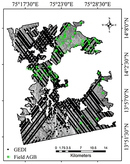
Figure 1. Shivamogga forest range image acquired by ALOS-2/PALSAR-2 (HV polarization), Karnataka. Green color circles represent field measured above-ground biomass plot locations and black dots shows the spatial distribution of GEDI footprints (showing transects of footprints after filtering).

FIGURE 2

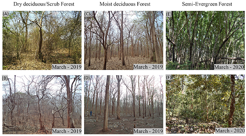
Figure 2. Photographs showing different forest types-(A) and (B) Dry deciduous or scrub forest, (C) and (D) Moist deciduous forest, and (E) and (F) Semi-Evergreen forest. The date of acquisition of the photographs is provided at the bottom right of each photo.

2.2. Data

2.2.1. Ground Reference Data

The in-situ measurements of the test site are collected during the field campaigns conducted in the dry season (March-April) of 2019 and 2020. For this study, we have measured forest parameters at 103 (31.6 × 31.6 m each) observation plots. In-situ forest parameters such as tree height, tree stem circumference at breast height (CBH), species information, and the number of trees are measured for each sample plot. All trees with circumference greater than 10 cm are measured to derive forest height and biomass in this study. The species-specific volumetric equations developed by Forest Survey of India (1996) are used to estimate the individual tree volume. Further, tree stem biomass is obtained by multiplying tree volume with its wood specific gravity (Chowdhury et al., 1958) and biomass expansion factor (BEF) (Haripriya, 2000). The sum of tree biomass within each sample plot provides a plot-level above-ground biomass estimate. In this study, the field plots that intercept both the ALOS-2/PALSAR-2 and Radarsat-2 acquisitions are considered for biomass modeling. The mean and standard deviation of biomass and stand height in the study area is 125.54 ± 60.90 Mg/ha and 16.07 ± 6.77 m, respectively. The statistics of various forest parameters collected during the field campaigns is shown in Table 1.

TABLE 1

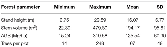
Table 1. Summary of forest parameter statistics collected during field campaigns (SD represents standard deviation).

2.2.2. SAR Data

Over Shivamogga, L-band ALOS-2/PALSAR-2 data and C-band Radarsat-2 data was acquired in 12-January-2019 and 08-March-2019. The ALOS-2/PALSAR-2 data is acquired in fine-resolution dual-polarized strip-map mode and provided in complex SLC (single look complex) format. The L-band data obtained has HH and HV polarization, with range and azimuth spacing of 4.29 and 3.40 m, and incidence-angle varying between 28.53^o and 33.95^o. The Radarsat-2 C-band acquired with FQ18 beam (Fine quad Polarization beam) over the study site have a range and azimuth resolution of 4.73 and 4.96 m, and the incidence angle range between 37.35^o and 38.86^o is obtained in SLC format. The details of the SAR data is given in Table 2.

TABLE 2

Table 2. The characteristics of SAR data utilized in this study.

2.2.3. LiDAR Data

Global Ecosystem Dynamics Investigation (GEDI) LiDAR operates from the Japanese Experimental Module's Exposed Facility (JEM-EF) on the International Space Station (ISS). GEDI LiDAR illuminates the earth surface using three laser pulses with a wavelength of 1064 nm at 242 Hz. The footprints of the GEDI laser pulse is approximately 25 m in diameter. GEDI swath has eight ground tracks with 60 m along-track resolution and 600 m across-track resolution. In this study, Level 2A (L2A) product that provides footprint-level elevation and canopy heights are used. The canopy height is calculated from the received waveform by subtracting the highest LiDAR wave return elevation from the ground return's elevation. The L2A product also includes height metrics, which measure height above the ground at each energy quantile in the received waveform (Dubayah et al., 2020). The GEDI LiDAR data used in this study is acquired between April 2019 and August 2021.

2.3. Method

SAR data acquired by ALOS-2/PALSAR-2 (L-band) and Radarsat-2 (C-band) and LiDAR footprints acquired by the GEDI platform are used to analyze the potential of combining these two data-sets for improvement in forest biomass retrieval. Random forest machine learning regression is used to develop biomass models. The overall approach followed in this research is shown in Figure 3, and the detailed methods are provided below.

FIGURE 3

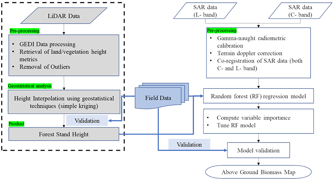
Figure 3. Flow chart showing the approach followed in the development of multi-frequency SAR and multi-temporal LiDAR data based AGB models.

2.3.1. SAR Data Pre-processing

The data from ALOS-2/PALSAR-2 and Radarsat-2 are obtained in SLC format. The pre-processing of SAR data involves radiometric calibration, normalization of backscatter using incidence angle (Small et al., 2010) [see Equation (1)], Multi-looking, terrain doppler correction, and co-registration of C- and L- band SAR data. The Radarsat-2 image is multi-looked with six looks in azimuth and four looks in range direction to generate ground range pixel of 30.23 m, and ALOS-2/PALSAR-2 image is multi-looked with eleven looks in azimuth and six looks in range direction to generate 33.82 m ground range pixel. The multi-looked images are geocoded using SRTM 1 Arc Sec DEM and resampled to 30 m pixel spatial resolution. The terrain corrected L- band and C- band data is further co-registered for multi-frequency SAR analysis.

$\begin{array}{ll}{\gamma }^o=\frac{{\sigma }^o}{cos\theta }& (1)\end{array}$

In equation 1, γ^o denote topographically corrected backscatter, σ^o represents radiometrically calibrated backscatter, and θ indicate local incidence angle.

2.3.2. LiDAR Data Pre-processing

GEDI LiDAR footprint data acquired over Shivamogga are obtained in Level -2 processed format from NASA EARTHDATA access portal (information to access data is provided in the URL (https://lpdaacsvc.cr.usgs.gov/services/gedifinder). The downloaded level 2A (L2A) GEDI canopy height product is processed using the rGEDI package (Silva et al., 2020) in R Software. Canopy relative height metrics (RH₀ to RH₁₀₀) and canopy flag are extracted from the L2A GEDI product. The canopy metric RH₁₀₀ is considered as the canopy height in this study. The LiDAR data is filtered to remove GEDI footprints that have uncertainty in canopy metric estimation (all LiDAR footprint data with canopy flag 0 are removed from this analysis). Based on the field campaign analysis, LiDAR footprints with canopy height less than 5 m and more than 40 m are excluded from the study, considering the range of stand height in the study area. Total GEDI footprints acquired over Shivamogga was 39,622, and after filtering the data to remove uncertain footprints, we obtained 21,405 GEDI footprints spatially distributed across Shivamogga (see Figure 1 for visualizing the spatial distribution of GEDI footprints).

2.3.3. Interpolation of GEDI Canopy Height Using the Geostatistical Method

Geostatistics is an advanced geographic interpolation technique that predicts unknown sample values by considering the area's characteristics surrounding the point of interest. By considering the spatially auto-correlated nature of the forests (Watham et al., 2016), an attempt is made to interpolate canopy height from GEDI LiDAR footprints using the spatial interpolation technique ordinary kriging. Considering the high density of GEDI footprints spatially distributed evenly across the study site in the form of strips, we implemented simple spatial modeling instead of widely used multi-variate geostatistical methods.

The geostatistical analysis is performed in ArcGIS (ver 10.1). The semi-variance analysis is performed with the Gaussian model to characterize the spatial auto-correlation of LiDAR footprint measurements. The interpolated forest stand height obtained from the simple kriging method is validated using 88 field sample plots and root mean squared error estimated.

2.3.4. Forest Aboveground Biomass Modeling

Random forest regression machine learning technique is used to model forest above-ground biomass. Three sets of different models with varying predictor variables are developed and is shown in Table 3. The first model is generated using only single-frequency SAR data (Separately for C-band and L-band) as predictor variables. At the same time, the second set of models utilize co-registered multi-frequency SAR data (from C-band and L-band) as predictor variables. The third set of models is developed from SAR (both single-frequency and multi-frequency) and LiDAR data. In this study, 75% of the ground samples are used for training, and the rest, 25% of samples, are used for validation. The study compares the models using rmse values to find the best performing models. In this study, various nomenclature representing forest above-ground biomass such as AGB or forest biomass or biomass are interchangeably used throughout this research paper.

TABLE 3

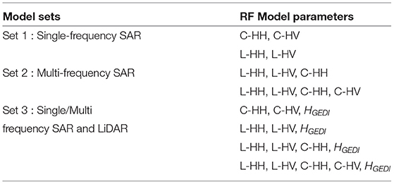
Table 3. Predictor variables used in the Random forest regression algorithm for forest aboveground biomass estimation in Shivamogga forest. H_GEDI represents the canopy height obtained from GEDI L2A product.

3. Results

3.1. Analyses of C-Band and L-Band SAR Backscatter and Its Saturation Limit

SAR backscatter from ALOS-2/PALSAR-2 and Radarsat-2 data was extracted for the geolocations of field measurement AGB plots. Scatter plots were used to relate field measured forest above-ground biomass and SAR backscatter from C-band and L-band, and a logarithmic relation curve is fit between them. The saturation limit is defined similar to Englhart et al. (2011), where the slope of the curve is estimated, and the saturation limit is set to the curve slope less than 0.1 dB. The logarithmic relationship between measured forest above-ground biomass and SAR data is shown in Figures 4A–D. The slope analysis resulted in a 74 Mg/ha saturation limit for C-band HH backscatter and 61 Mg/ha for C-band HV backscatter (see Figures 4A,B). The L-band SAR backscatter showed a higher saturation limit with 120 Mg/ha for HH polarization and 168 Mg/ha for HV polarization (see Figures 4C,D).

FIGURE 4

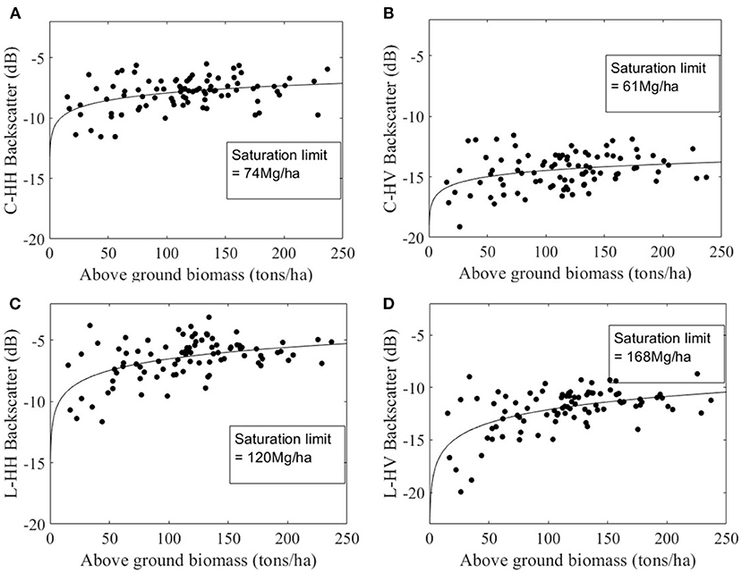
Figure 4. Saturation limit of SAR backscatter with forest above-ground biomass. (A) and (B) shows the scatterplot of HH and HV backscatter of C-band data from Radarsat2 acquired on 08-Mar-2019, (C) and (D) shows the saturation limit of L-band data from ALOS-2/PALSAR-2 acquired on 12-Jan-2019.

3.2. Interpolation of Forest Height From LiDAR Footprint

GEDI LiDAR platform receives the transmitted waves and measures three-dimensional properties of forest structure in an evenly distributed spatial extent. The forest regions without the LiDAR footprint lacks measurement and causes gaps in LiDAR outputs. These measurement gaps are filled using the spatial interpolation technique. A simple kriging method was used to interpolate canopy height metric RH₁₀₀ spatially and forest stand height predicted for the forest region. In previous studies, the univariate kriging technique has not performed well in predicting forest variables (Watham et al., 2016) due to the lower number of measurements available for geostatistical modeling. However, the high density of GEDI LiDAR footprints over the study area provides an opportunity to overcome the above drawback. The forest canopy height interpolation using the simple kriging technique performed better with an R² of 0.77 and root mean squared error of 4.71 m. The spatial prediction map of forest canopy height for the study site and its validation scatterplot with a 1:1 line and 20% error limit is shown in Figure 5. The result shows a slight overestimation in canopy height for forest stands with a height less than 15 m. This overestimation might be due to the undulating terrain in the study area and might also be due to the significant gaps in LiDAR footprints across-track direction.

FIGURE 5

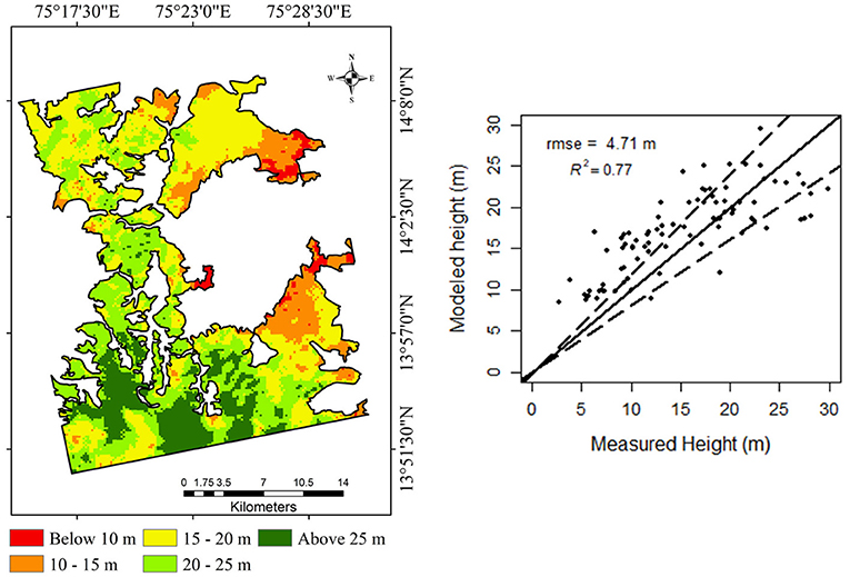
Figure 5. Validation of simple kriging interpolated GEDI forest stand height. The solid black line shows a 1:1 line and the dotted lines indicate a 20% error limit.

3.3. Forest Above-Ground Biomass Modeling

The random forest regression technique modeled the forest aboveground biomass using different variables. Initially, the model was developed with single-frequency SAR data from C-band and L-band data with HH and HV polarization channels as predictor variables. Then the model developed included predictor variables from multi-frequency SAR data and a combination of co-registered multi-frequency SAR and interpolated LiDAR canopy height data. The results obtained are shown in the following subsections.

3.3.1. Forest AGB From Single-Frequency and Multi-Frequency SAR Data

Single-frequency SAR data backscatter from C-band Radarsat-2 and L-band ALOS-2/PALSAR-2 were used as predictor variables in the retrieval of forest above-ground biomass. A random forest regression model was developed with a nTree (Number of decision trees) of 500 and out-of-bag (OOB) error estimated for the decision trees. The analysis shows that the OOB error curve flattens after 200 decision trees. Then, the random forest model was fine-tuned with nTree value of 200 and the forest above-ground biomass model was developed with 75% training samples. Modeled forest above-ground biomass is validated using the rest of 25% of testing samples. Results obtained show that the model developed from L-band SAR backscatter performed better with a %rmse of 25.06 than the C-band data, which performed with a %rmse of 32.08 (see Figures 6A,B).

FIGURE 6

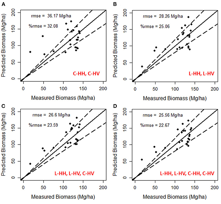
Figure 6. Validation of modeled forest above-ground biomass derived from Random Forest regression models on (A) L-band backscatter, (B) C-band backscatter, (C) combination of L-${\gamma }_{HH}^0$, L-${\gamma }_{HV}^0$, and C-${\gamma }_{HV}^0$, and (D) combination of L-band and C-band backscatter. Dotted lines show the 20% error limit.

SAR data (HH and HV polarization only) from Radarsat-2 and ALOS-2/PALSAR-2 are co-registered to perform a multi-frequency SAR analysis for forest above-ground biomass estimation. The random forest regression algorithm used the co-registered multi-frequency SAR data as predictor variables. Similar to analysis in single-frequency SAR, a random forest regression algorithm is developed, and variable importance for the multi-frequency SAR data is estimated. For this multi-frequency analysis, the order of variable importance in descending sequence for the model developed is L-HV, L-HH, C-HV, and C-HH. The addition of C-HV backscatter to L-band data improved the estimation accuracy with a decrease of relative rmse (%rmse) from 25.06 to 23.59% (see Figure 6C). Further addition of C-HH polarization further improved the estimation accuracy with a %rmse of 22.67 (Figure 6D). Estimating forest biomass from this multi-frequency model improved the estimation accuracy compared to single-frequency SAR-based estimation.

3.3.2. Combining LiDAR and Single/Multi-Frequency SAR Data for Forest AGB Retrieval

Interpolated GEDI LiDAR canopy height raster image of the study site (see section 3.2 Interpolation of forest height from LiDAR footprint) was co-registered with multi-frequency SAR data, and their values co-located to field measurements are extracted. Seventy-five percent of these extracted values are used to train the random forest regression algorithm. Similar to the results obtained in section Forest AGB from single-frequency and multifrequency SAR data, variable importance among the training samples is estimated. The canopy height layer showed the highest significance among the variables, followed by L-HV, L-HH, C-HV, and C-HH for biomass estimation. As elaborated in section Forest AGB from single-frequency and multifrequency SAR data, number of trees were fine tuned to 200 following the analysis of OOB error. Figures 7A–D shows the modeled biomass estimates obtained from this hybrid stack.

FIGURE 7

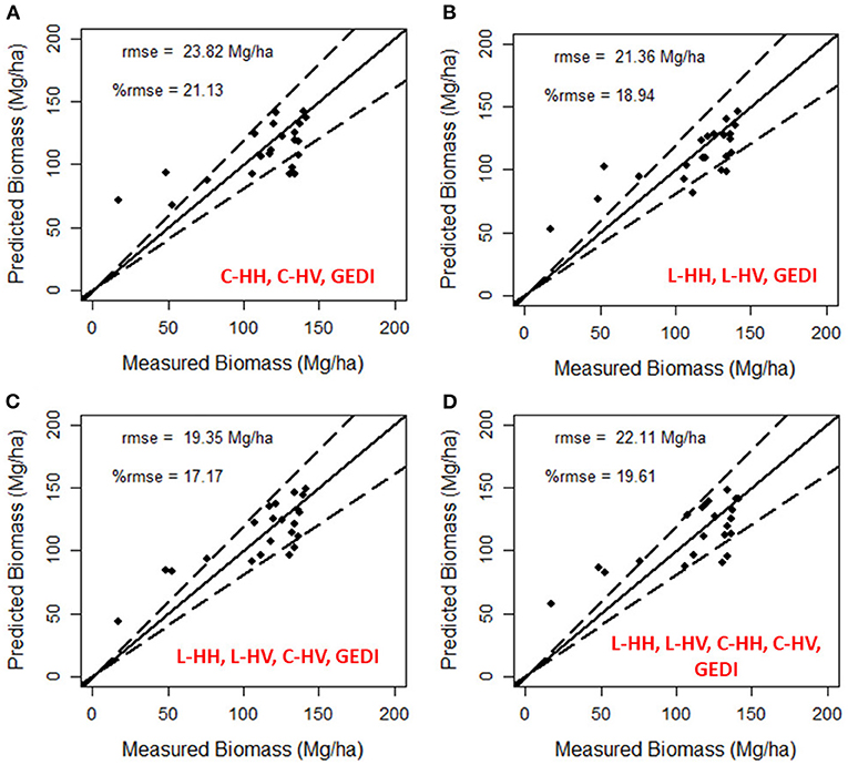
Figure 7. Validation of modeled AGB using multi-frequency SAR data and interpolated LiDAR canopy height data. The model performance of different combinations is shown in (A) L-band SAR data and LiDAR, (B) C-band SAR data and LiDAR, and (C,D) showing the combination of C- and L-band SAR with LiDAR data. The dotted lines show a 20% error limit.

The inclusion of canopy height in the random forest model improved the above-ground biomass estimation in single-frequency and multi-frequency SAR-based methods. The modeled biomass is validated with the ground truth testing data and their relative rmse (%rmse) estimated. Among the single-frequency SAR and LiDAR data combination, L-band data performed better with a relative rmse of 18.94%, while the C-band data resulted in a relative rmse of 21.13%. By comparing the modeled biomass estimates from L-band data (see Figures 6B, 7B), integration of canopy height reduced the relative rmse from 25.06 to 18.94%. The modeled biomass from multi-frequency SAR and canopy height reduces the error, thereby improving the estimation accuracy. The validation of the modeled above-ground biomass resulted in a relative rmse of 17.17% (Figure 7C) for L-HH, L-HV, C-HV, and GEDI, and 19.61% (Figure 7D) for all bands of L-band and C-band data along with GEDI canopy height. Removal of the least important variable among the predictor variable improved the accuracy in multi-frequency SAR and GEDI models. At the same time, no such improvement is observed in the multi-frequency SAR based model (see Figures 6C,D). A forest above-ground biomass map is generated for the best performing model with the least relative rmse of 17.17% is shown in Figure 8.

FIGURE 8

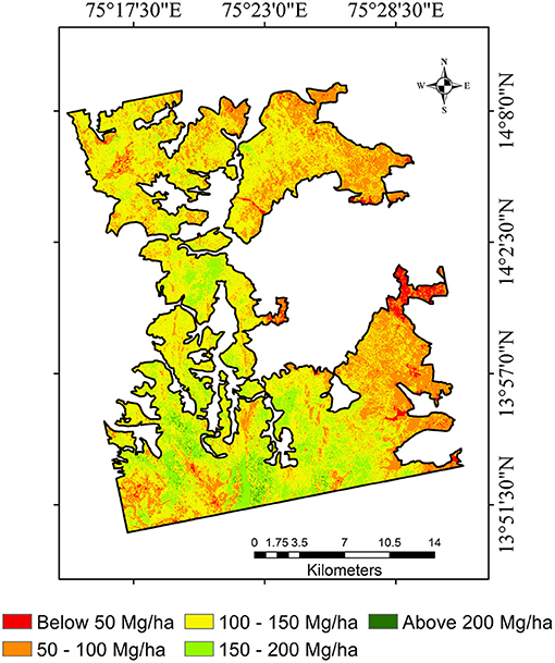
Figure 8. Forest aboveground biomass map generated from the best performing RF model with predictor variables - L-${\gamma }_{HH}^0$, L-${\gamma }_{HV}^0$, C-${\gamma }_{HV}^0$, and GEDI canopy heights.

The biomass map shows the spatial distribution of different densities of biomass across the study site. Low biomass spatial distribution is observed in the east side and the study site's peripheral borders. This might be due to enhanced anthropological pressure since these areas have settlements bordering. Also, despite being a protected forest, the peripheral regions show signs of forest degradation, while a high biomass range is observed in the intact forest regions of the study site.

4. Discussion

This study analyses the potential of the combination of SAR data acquired in different frequencies and LiDAR footprints in retrieving forest above-ground biomass over tropical forest regions. Forest biomass is retrieved from L-band ALOS-2/PALSAR-2 data and C-band Radarsat-2 data individually and combinedly. Further, the SAR and LiDAR data were integrated, and models were developed using a random forest machine-learning algorithm.

The results obtained shows L-band data showed high estimation accuracy than C-band data similar to the earlier observations in other tropical forest regions (Nizalapur et al., 2010). SAR backscatter from L-band and C-band interacts with different parts of the trees. The high-frequency C-band data mainly interacts with leaves and tertiary branches, while the low-frequency L-band data interacts with secondary branches and tree trunk (Le Toan et al., 1992; Ranson and Guoqing Sun, 1994; Englhart et al., 2011). Joshi et al. (2017) analyzed the causes for the difference in backscatter and saturation limit and observed that the backscatter signals tends to decrease with an increase in vertical canopy opacity, stem density, and understorey vegetation, which results in lower sensitivity towards forest biomass. Even though the study area has high species diversity consisting of 66 different tree species with varying vertical canopy height, which favors low backscatter and low saturation limit, the climatic conditions during the acquisition of SAR data favor abscission (leaf-fall). This leafless condition, along with dry climatic conditions, results in low canopy density and negligible understory vegetation, which increases the SAR backscatter and results in high sensitivity towards forest biomass. This low canopy density condition resulted in considerable surface-trunk inter-action in C-band HH polarization and so high saturation limit than the C-HV band. The saturation limit of 74 and 61 Mg/ha for HH and HV polarization of C-band data is reported in this study concurs with the previous observations made in Indian tropical forests where the saturation limit was observed between 60–70 Mg/ha (Nizalapur et al., 2010). However, L-band data showed high saturation limit (120 Mg/ha for HH polarization and 168 Mg/ha for HV polarization) than other reported studies over tropical forests where the saturation limit varied between 50 to 150 Mg/ha for HV polarization (Nizalapur et al., 2010; Englhart et al., 2011; Sandberg et al., 2011).

The forest above-ground biomass estimated using single frequency SAR data showed L-band data performing better than C-band data (see Figures 6A,B). This is because of the canopy penetration capability of the L-band signal and its inter-action with secondary branches and the main trunk where the majority of the biomass is stored. Whereas C-band signals mostly interact with secondary and tertiary branches and saturate with an increase in canopy density, thereby less sensitive to biomass retrieval. Existing literature (Englhart et al., 2011; Cartus and Santoro, 2019) showed that combining low and high-frequency SAR data improves the forest biomass estimates since the combination accounts for more interaction of SAR signal towards forest biomass components such as leaves, tertiary branches, secondary branches and main trunk. Forest aboveground biomass retrieval accuracy improved by combining C-band and L-band data (see Figures 6C,D). In the random forest regression algorithm, the importance of the predictor variables was estimated, and for this analysis, C-HH polarization showed the least importance in the multiple frequency SAR data based above-ground biomass modeling. However, removing the least important variable has not improved the result. In contrast, the removal of C-HH polarization increased the relative rmse from 22.67% to 23.59%. This phenomenon is because HH polarization mainly interacts with the surface-trunk backscattering component, which accounts for the long vertical structure where most of the biomass is stored.

Canopy height was provided as an input to the random forest algorithm along with single or multiple frequencies SAR data to model forest above-ground biomass in this study. The canopy height of the study site was obtained from the GEDI LiDAR platform. The filtering of the GEDI data was performed to remove the sources of error at the pre-processing stage. Since the GEDI platform measures the canopy properties at the footprint level, it has gaps in across-track and along-track directions. These gaps are filled with interpolated values using the geostatistical univariate simple kriging method. Even though previous studies showed lower performance due to low-density sampling points (Watham et al., 2016), the current study performed comparatively better because of dense GEDI spatial distribution and spatial auto-correlation of forests. The overall accuracy of the interpolated canopy height performed better with a rmse of 4.71 m. In order to analyze the accuracy of interpolated canopy height at those areas where GEDI footprints are unavailable, we performed a geospatial analysis in which field AGB points farther than 500 m from GEDI footprints were segregated. A comparison of height validation in terms of rmse is performed for these segregated points and for those ground truth points which have a set of GEDI footprints in their vicinity. There were 26 estimates present in the segregated zone and 62 points in the GEDI footprint zone. The scatter plot for these two sets of height validation is shown in Figures 9A,B.

FIGURE 9

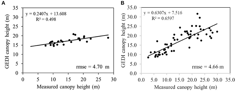
Figure 9. (A) Showing the scatter plot for ground truth points in the non-GEDI footprint region (26 points) and (B) shows the validation plot for ground truth located in the vicinity of GEDI footprints (62 points).

The validation of interpolated GEDI in regions having LiDAR footprints within 500 m vicinities and otherwise shows that the error in the model is stable, meaning the interpolated canopy height from geostatistical kriging has less error deviation across the study site. Our rmse values is similar to what (Guerra-Hernández and Pascual, 2021) reported (rmse = 4.45 m) and higher than the values showed by Silva et al. (2021) (rmse = 3.7 m). The overall rmse obtained in this study is high because of the heterogeneous canopy condition (high species diversity) and varying topography of the study site. This study reflects that the inclusion of forest canopy height with backscatter from either single/multiple frequencies provided better accuracy for forest biomass prediction. The variable importance analysis of the predictor variables in random forest regression shows the canopy height as the most important variable in explaining forest above-ground biomass. Previous literature has emphasized using multi-temporal SAR data to eliminate the effects due to environmental conditions (Englhart et al., 2011; Cartus and Santoro, 2019); it has not been implemented in this study due to the unavailability of Radarsat-2 data over the study area. However, incorporation of canopy height to the biomass model (L-HH, L-HV, C-HV) improved the relative rmse from 23.59% to 17.17% (see Figures 6C, 7C). Even for all the polarization combinations, incorporation of LiDAR data have improved the accuracy of the biomass estimation; from 32.08% to 21.13% for C-band, 25.06% to 18.94% for L-band, and 22.67% to 19.61% for all channels of L- and C-band data, respectively (see Figures 6, 7). The longer wavelength L-band data combined with GEDI data provided better results with rmse less than 20%, which is an acceptable error range for the NISAR mission.

In most studies, where LiDAR data is used to calibrate with field biomass, the relationship obtained estimates biomass at the LiDAR footprint level. Further, these calibrated footprint level biomass is used as ground truth samples and further used in modeling biomass using SAR data. In these studies, the spatial resolution of LiDAR footprints, field plots, and SAR data might cause edge-effect when their spatial resolution is smaller (Berninger et al., 2018). The current study reduces the uncertainty associated with spatial resolution of satellite imagery and field plots for forest biomass estimation as the GEDI LiDAR footprints are converted into a continuous height layer by interpolation and then coregistered with SAR data. The error due to smaller pixel size is limited to geolocation error of field plots caused by the horizontal accuracy of GPS receiver. Therefore, larger field plots (≥1ha) should be planned in future field campaigns in order to reduce the errors due to coregistration and spatial averaging.

5. Conclusion

The study has successfully demonstrated the quantification of forest AGB in one of the highly diverse tropical hotspots in the Western Ghats in India. The study showed that the combination of L-band SAR data (HH and HV polarization), C-band (HV polarization), and GEDI LiDAR canopy heights have high sensitivity to forest biomass. Analysis of the impact of canopy height error bias on forest above-ground biomass estimation will be considered in future studies. The approach developed would serve as one of the frameworks in the upcoming time series dual-frequency SAR mission NISAR and other higher wavelength SAR missions ALOS-4 and BIOMASS. More research is required in analyzing the utility of multi-temporal and multi-frequency SAR data for forest biomass estimation in very high biomass regions of the tropical forest. The inclusion of canopy height has shown promising improvement in forest aboveground biomass estimation. However, more research is required to integrate canopy height variables from different LiDAR missions like ICESat-2, GEDI and upcoming MOLI to improve the accurate estimation of forest biomass.

Data Availability Statement

The datasets presented in this article are not readily available because. The distribution of SAR and field raw data supporting the conclusion of this study is restricted because of project agreements between the authors and the data providers. Requests to access the datasets should be directed to gulab.singh@iitb.ac.in.

Author Contributions

MM and GS: conceptualization and methodology. MM: data curation, processing and analysis, fieldwork collection, and writing—original draft preparation. GS: infrastructure support, writing—review and editing, supervision, project administration, and funding acquisition. All authors contributed to the article and approved the submitted version.

Funding

This research work was partially funded by the Indian Space Research Organization under the research announcement for the NISAR project coded Eco-05.

Conflict of Interest

The authors declare that the research was conducted in the absence of any commercial or financial relationships that could be construed as a potential conflict of interest.

Publisher's Note

All claims expressed in this article are solely those of the authors and do not necessarily represent those of their affiliated organizations, or those of the publisher, the editors and the reviewers. Any product that may be evaluated in this article, or claim that may be made by its manufacturer, is not guaranteed or endorsed by the publisher.

Acknowledgments

We would like to thank Japan Aerospace Exploration Agency (JAXA) for providing ALOS-2/PALSAR-2 datasets over the study site under the project JAXA-3056 and the Canadian Space Agency for providing Radarsat-2 data under the project SOAR-5449. The authors are immensely grateful to Mr. Surya Sen IFS, Mr. A. S. Mariappa IFS, Mr. G. U. Shankar SFS, Ms. Deepika IFS, Mr. Nagaraja N. P. Dy.RFO, Niranjan S. P. Dy.RFO, Manjunath K. N. Dy.RFO, and other forest officers for providing extended support during the field campaigns at Shivamogga forest division. We are also grateful to the support extended by the researchers Mr. B. R. Nela, Mr. G. Dasondhi, Mr. A. Sheikh, and Mr. A. Chandra during the field campaigns.

References

Askne, J., Fransson, J., Santoro, M., Soja, M., and Ulander, L. (2013). Model-based biomass estimation of a hemi-boreal forest from multitemporal TanDEM-X acquisitions. Rem. Sens. 5, 5574–5597. doi: 10.3390/rs5115574

CrossRef Full Text | Google Scholar

Askne, J., and Santoro, M. (2007). Selection of forest stands for stem volume retrieval from stable ERS tandem InSAR observations. IEEE Geosci. Rem. Sens. Lett. 4, 46–50. doi: 10.1109/LGRS.2006.883525

PubMed Abstract | CrossRef Full Text | Google Scholar

Askne, J., and Santoro, M. (2012). “Experiences in boreal forest stem volume estimation from multitemporal C-Band InSAR,” in Recent Interferometry Applications in Topography and Astronomy, ed I. Padron (IntechOpen). Available online at: https://www.intechopen.com/chapters/33100 (accessed March 21, 2012).

Google Scholar

Behera, M., Tripathi, P., Mishra, B., Kumar, S., Chitale, V., and Behera, S. K. (2016). Above-ground biomass and carbon estimates of Shorea robusta and Tectona grandis forests using QuadPOL ALOS PALSAR data. Adv. Space Res. 57, 552–561. doi: 10.1016/j.asr.2015.11.010

CrossRef Full Text | Google Scholar

Berninger, A., Lohberger, S., StÃngel, M., and Siegert, F. (2018). Sar-based estimation of above-ground biomass and its changes in tropical forests of kalimantan using l- and c-band. Rem. Sens. 10:831. doi: 10.3390/rs10060831

CrossRef Full Text | Google Scholar

Cartus, O., and Santoro, M. (2019). Exploring combinations of multi-temporal and multi-frequency radar backscatter observations to estimate above-ground biomass of tropical forest. Rem. Sens. Environ. 232:111313. doi: 10.1016/j.rse.2019.111313

CrossRef Full Text | Google Scholar

Cartus, O., Santoro, M., and Kellndorfer, J. (2012). Mapping forest aboveground biomass in the Northeastern United States with ALOS PALSAR dual-polarization L-band. Rem. Sens. Environ. 124, 466–478. doi: 10.1016/j.rse.2012.05.029

CrossRef Full Text | Google Scholar

Cartus, O., Santoro, M., Wegmuller, U., and Rommen, B. (2017). “Estimating total aboveground, stem and branch biomass using multi-frequency SAR,” in 2017 9th International Workshop on the Analysis of Multitemporal Remote Sensing Images (MultiTemp) (Brugge: IEEE), 1–3.

Google Scholar

Chowdhury, K., Ghosh, S., Rao, K., and Branch, F. R. I. W. A. (1958). “Number v. 3 in Indian Woods: their identification, properties and uses,” in Indian Woods: Their Identification, Properties and Uses. (Delhi: Manager of Publications).

Chowdhury, T. A., Thiel, C., and Schmullius, C. (2014). Growing stock volume estimation from L-band ALOS PALSAR polarimetric coherence in Siberian forest. Rem. Sens. Environ. 155, 129–144. doi: 10.1016/j.rse.2014.05.007

CrossRef Full Text | Google Scholar

Dhanda, P., Nandy, S., Kushwaha, S., Ghosh, S., Murthy, Y. K., and Dadhwal, V. (2017). Optimizing spaceborne LiDAR and very high resolution optical sensor parameters for biomass estimation at ICESat/GLAS footprint level using regression algorithms. Progr. Phys. Geography Earth Environ. 41, 247–267. doi: 10.1177/0309133317693443

CrossRef Full Text | Google Scholar

Dobson, M., Ulaby, F., Pierce, L., Sharik, T., Bergen, K., Kellndorfer, J., et al. (1995). Estimation of forest biophysical characteristics in Northern Michigan with SIR-C/X-SAR. IEEE Trans. Geosci. Rem. Sens. 33, 877–895. doi: 10.1109/36.406674

PubMed Abstract | CrossRef Full Text | Google Scholar

Dubayah, R., Blair, J. B., Goetz, S., Fatoyinbo, L., Hansen, M., Healey, S., et al. (2020). The Global ecosystem dynamics investigation: high-resolution laser ranging of the Earth's forests and topography. Sci. Rem. Sens. 1:100002. doi: 10.1016/j.srs.2020.100002

CrossRef Full Text | Google Scholar

Duncanson, L., Neuenschwander, A., Hancock, S., Thomas, N., Fatoyinbo, T., Simard, M., et al. (2020). Biomass estimation from simulated GEDI, ICESat-2 and NISAR across environmental gradients in Sonoma County, California. Rem. Sens. Environ. 242:111779. doi: 10.1016/j.rse.2020.111779

CrossRef Full Text | Google Scholar

Englhart, S., Keuck, V., and Siegert, F. (2011). Aboveground biomass retrieval in tropical forests - the potential of combined X- and L-band SAR data use. Rem. Sens. Environ. 115, 1260–1271. doi: 10.1016/j.rse.2011.01.008

CrossRef Full Text | Google Scholar

Feng, Q., Zhou, L., Chen, E., Liang, X., Zhao, L., and Zhou, Y. (2017). The performance of airborne C-band PolInSAR data on forest growth stage types classification. Rem. Sens. 9:955. doi: 10.3390/rs9090955

CrossRef Full Text

Forest Survey of India (1996). Volume Equations for Forests of India, Nepal, and Bhutan. Forest Survey of India, Ministry of Environment & Forests, Government of India, Dehradun.

Gibbs, H. K., Brown, S., Niles, J. O., and Foley, J. A. (2007). Monitoring and estimating tropical forest carbon stocks: making REDD a reality. Environ. Res. Lett. 2:045023. doi: 10.1088/1748-9326/2/4/045023

CrossRef Full Text | Google Scholar

Guerra-Hernández, J., and Pascual, A. (2021). Using GEDI lidar data and airborne laser scanning to assess height growth dynamics in fast-growing species: a showcase in Spain. Forest Ecosyst. 8:14. doi: 10.1186/s40663-021-00291-2

CrossRef Full Text | Google Scholar

Haripriya, G. S. (2000). Estimates of biomass in Indian forests. Biomass Bioenergy 19, 245–258. doi: 10.1016/S0961-9534(00)00040-4

PubMed Abstract | CrossRef Full Text | Google Scholar

Houghton, R. A., Hall, F., and Goetz, S. J. (2009). Importance of biomass in the global carbon cycle. J. Geophys. Res. Biogeosci. 114:G00E03. doi: 10.1029/2009JG000935

CrossRef Full Text | Google Scholar

Joshi, N., Mitchard, E. T. A., Brolly, M., Schumacher, J., Fernández-Landa, A., Johannsen, V. K., et al. (2017). Understanding 'saturation' of radar signals over forests. Sci. Rep. 7:3505. doi: 10.1038/s41598-017-03469-3

PubMed Abstract | CrossRef Full Text

Khati, U., Singh, G., and Ferro-Famil, L. (2017). Analysis of seasonal effects on forest parameter estimation of Indian deciduous forest using TerraSAR-X PolInSAR acquisitions. Rem. Sens. Environ. 199, 265–276. doi: 10.1016/j.rse.2017.07.019

CrossRef Full Text | Google Scholar

Kim, C. (2012). Quantataive analysis of relationship between ALOS PALSAR backscatter and forest stand volume. J. Marine Sci. Technol. 20, 624–628. doi: 10.6119/JMST-012-0402-1

CrossRef Full Text | Google Scholar

Kugler, F., Lee, Seung-Kuk, Hajnsek, I., and Papathanassiou, K. P. (2015). Forest height estimation by means of pol-InSAR data inversion: the role of the vertical wavenumber. IEEE Trans. Geosci. Rem. Sens. 53, 5294–5311. doi: 10.1109/TGRS.2015.2420996

PubMed Abstract | CrossRef Full Text | Google Scholar

Kumar, S., Pandey, U., Kushwaha, S. P. S., Chatterjee, R. S., and Bijker, W. (2012). Aboveground biomass estimation of tropical forest from Envisat ASAR data using modeling approach. J. Appl. Rem. Sens. 6:18. doi: 10.1117/1.JRS.6.063588

PubMed Abstract | CrossRef Full Text

Kuplich, T. M., Curran, P. J., and Atkinson, P. M. (2005). Relating SAR image texture to the biomass of regenerating tropical forests. Int. J. Rem. Sens. 26, 4829–4854. doi: 10.1080/01431160500239107

CrossRef Full Text | Google Scholar

Le Toan, T., Beaudoin, A., Riom, J., and Guyon, D. (1992). Relating forest biomass to SAR data. IEEE Trans. Geosci. Rem. Sens. 30, 403–411.

Google Scholar

Lu, D. (2006). The potential and challenge of remote sensing-based biomass estimation. Int. J. Rem. Sens. 27, 1297–1328. doi: 10.1080/01431160500486732

CrossRef Full Text | Google Scholar

Malhi, Y., Meir, P., and Brown, S. (2002). Forests, carbon and global climate. Philosoph. Trans. Roy. Soc. London. Series A Math. Phys. Eng. Sci. 360, 1567–1591. doi: 10.1098/rsta.2002.1020

PubMed Abstract | CrossRef Full Text | Google Scholar

Mitchard, E. T. A., Saatchi, S. S., Woodhouse, I. H., Nangendo, G., Ribeiro, N. S., Williams, M., et al. (2009). Using satellite radar backscatter to predict above-ground woody biomass: A consistent relationship across four different African landscapes. Geophys. Res. Lett. 36:L23401. doi: 10.1029/2009GL040692

CrossRef Full Text | Google Scholar

Musthafa, M., Khati, U., and Singh, G. (2020). Sensitivity of PolSAR decomposition to forest disturbance and regrowth dynamics in a managed forest. Adv. Space Res. 66, 1863–1875. doi: 10.1016/j.asr.2020.07.007

CrossRef Full Text | Google Scholar

Musthafa, M., and Singh, G. (2019). “Potential of Alpha angle of fully polarimetric L-band data time series in characterizing forest dynamics,” in IGARSS 2019 - 2019 IEEE International Geoscience and Remote Sensing Symposium (Yokohama: IEEE), 5925–5928.

Google Scholar

Nandy, S., Srinet, R., and Padalia, H. (2021). “Mapping forest height and aboveground biomass by integrating ICESat-2, sentinel-1 and sentinel-2 data using random forest algorithm in northwest himalayan foothills of India. Geophys. Res. Lett. 48:e2021GL093799. doi: 10.1029/2021GL093799

CrossRef Full Text

Narine, L. L., Popescu, S., Neuenschwander, A., Zhou, T., Srinivasan, S., and Harbeck, K. (2019). Estimating aboveground biomass and forest canopy cover with simulated ICESat-2 data. Rem. Sens. Environ. 224, 1–11. doi: 10.1016/j.rse.2019.01.037

CrossRef Full Text | Google Scholar

Nizalapur, V., Jha, C., and Madugundu, R. (2010). Estimation of above ground biomass in Indian tropical forested area using multi-frequency DLR-ESAR data. Int. J. Geom. Geosci. 1, 167–178. Available online at: https://citeseerx.ist.psu.edu/viewdoc/download?doi=10.1.1.295.9454&rep=rep1&type=pdf

Google Scholar

Ranson, K., and Sun, Guoqing (1994). Mapping biomass of a northern forest using multifrequency SAR data. IEEE Trans. Geosci. Rem. Sens. 32, 388–396. doi: 10.1109/36.295053

PubMed Abstract | CrossRef Full Text | Google Scholar

Rodrí-guez-Veiga, P., Wheeler, J., Louis, V., Tansey, K., and Balzter, H. (2017). Quantifying forest biomass carbon stocks from space. Curr. Forestry Rep. 3, 1–18. doi: 10.1007/s40725-017-0052-5

PubMed Abstract | CrossRef Full Text | Google Scholar

Saatchi, S., Halligan, K., Despain, D. G., and Crabtree, R. L. (2007). Estimation of forest fuel load from radar remote sensing. IEEE Trans. Geosci. Rem. Sens. 45, 1726–1740. doi: 10.1109/TGRS.2006.887002

PubMed Abstract | CrossRef Full Text | Google Scholar

Sandberg, G., Ulander, L., Fransson, J., Holmgren, J., and Le Toan, T. (2011). L- and P-band backscatter intensity for biomass retrieval in hemiboreal forest. Rem. Sens. Environ. 115, 2874–2886. doi: 10.1016/j.rse.2010.03.018

CrossRef Full Text | Google Scholar

Santi, E., Paloscia, S., Pettinato, S., Fontanelli, G., Mura, M., Zolli, C., et al. (2017). The potential of multifrequency SAR images for estimating forest biomass in Mediterranean areas. Rem. Sens. Environ. 200, 63–73. doi: 10.1016/j.rse.2017.07.038

CrossRef Full Text | Google Scholar

Santoro, M., Askne, J., Smith, G., and Fransson, J. E. (2002). Stem volume retrieval in boreal forests from ERS-1/2 interferometry. Rem. Sens. Environ. 81, 19–35. doi: 10.1016/S0034-4257(01)00329-7

CrossRef Full Text | Google Scholar

Shugart, H. H., Saatchi, S., and Hall, F. G. (2010). Importance of structure and its measurement in quantifying function of forest ecosystems. J. Geophys. Res. Biogeosci. 115, 1–6. doi: 10.1029/2009JG000993

CrossRef Full Text | Google Scholar

Silva, C. A., Duncanson, L., Hancock, S., Neuenschwander, A., Thomas, N., Hofton, M., et al. (2021). Fusing simulated GEDI, ICESat-2 and NISAR data for regional aboveground biomass mapping. Rem. Sens. Environ. 253:112234. doi: 10.1016/j.rse.2020.112234

CrossRef Full Text | Google Scholar

Silva, C. A., Hamamura, C., Valbuena, R., Hancock, S., Cardil, A., Broadbent, E. N., et al. (2020). rGEDI: NASA's Global Ecosystem Dynamics Investigation (GEDI) Data Visualization and Processing. Version 0.1.9. Available online at: https://CRAN.R-project.org/package=rGEDI (accessed October 22, 2020).

Small, D., Miranda, N., Zuberbühler, L., Schubert, A., and Meier, E. (2010). Terrain-Corrected Gamma: Improved Thematic Land-Cover Retrieval for SAR With Robust Radiometric Terrain Correction. Bergen: ESA Living Planet Symposium. Available online at: https://www.zora.uzh.ch/id/eprint/41236/1/Small_Zuberbuehler_Terrain-corrected_Gamma_2010.pdf (accessed July 02, 2020).

Google Scholar

Stankevich, S. A., Kozlova, A. A., Piestova, I. O., and Lubskyi, M. S. (2017). “Leaf area index estimation of forest using sentinel-1 C-band SAR data,” in 2017 IEEE Microwaves, Radar and Remote Sensing Symposium (MRRS) (Kiev: IEEE), 253–256.

Google Scholar

Sun, G., Ranson, K., and Kharuk, V. (2002). Radiometric slope correction for forest biomass estimation from SAR data in the Western Sayani Mountains, Siberia. Rem. Sens. Environ. 79, 279–287. doi: 10.1016/S0034-4257(01)00279-6

CrossRef Full Text | Google Scholar

Thapa, R. B., Watanabe, M., Motohka, T., and Shimada, M. (2015). Potential of high-resolution ALOS-PALSAR mosaic texture for aboveground forest carbon tracking in tropical region. Rem. Sens. Environ. 160, 122–133. doi: 10.1016/j.rse.2015.01.007

CrossRef Full Text | Google Scholar

Thiel, C., and Schmullius, C. (2016). The potential of ALOS PALSAR backscatter and InSAR coherence for forest growing stock volume estimation in Central Siberia. Rem. Sens. Environ. 173, 258–273. doi: 10.1016/j.rse.2015.10.030

CrossRef Full Text | Google Scholar

Watham, T., Kushwaha, S. P., Nandy, S., Patel, N., and Ghosh, S. (2016). Forest carbon stock assessment at Barkot Flux tower Site (BFS) using field inventory, Landsat-8 OLI. Int. J. Multidiscipl. Res. Develop. 3, 111–119. Available online at: https://www.allsubjectjournal.com/search?keyword=Watham