 Robert Bagchi
 Michael C. LaScaleia
 Valerie R. Milici
 Dipanjana Dalui
95% of researchers rate our articles as excellent or good
Learn more about the work of our research integrity team to safeguard the quality of each article we publish.
Find out more
METHODS article
Front. For. Glob. Change , 29 April 2022
Sec. Forest Growth
Volume 5 - 2022 | https://doi.org/10.3389/ffgc.2022.810010
The analysis of spatial point patterns has greatly advanced our understanding of ecological processes. However, the methods currently available for analyzing replicated spatial point patterns (RSPPs) are rarely used by ecologists. One barrier to the use of RSPP analyses is a lack of software to implement the approaches that have been developed in the statistical literature. Here, we provide a practical guide to RSPP analysis and introduce the RSPPlme4 R package that implements the approaches we discuss. The methods we outline use a linear modeling framework to link variation in the spatial structure of point patterns to discrete and continuous explanatory covariates. We describe methods for linear models and mixed-effects models of RSPPs, including approaches to estimating confidence intervals via semi-parametric bootstrapping. The syntax for model fitting is similar to that used in linear and linear mixed-effects modeling packages in R. The RSPPlme4 package also allows users to easily plot the results of model fits. We hope that this tutorial will make methods for RSPP analysis accessible to a wide range of ecologists and open new avenues for gaining insight into ecological processes from spatial data.
The spatial arrangement of organisms influences population and community dynamics (Bolker and Pacala, 1997; Law and Dieckmann, 2000). In turn, many ecological processes leave a spatial signature that can be used to detect and quantify those processes (Murrell and Law, 2002; Wiegand and Moloney, 2004; Law et al., 2009; Wiegand et al., 2021). For example, seed dispersal syndromes can be detected from the clustering of trees (Seidler and Plotkin, 2006) and local conspecific negative density dependence, a signal of stabilizing coexistence, can be indicated by a decrease in spatial clustering of adult trees relative to juveniles (Getzin et al., 2008; Bagchi et al., 2011). Spatial analyses are particularly useful for understanding sessile organisms, such as trees, for which spatial structure may be particularly influential.
The distributions of sessile organisms through space are often represented using spatial point patterns: the spatial locations of individuals (e.g., latitude and longitude). These points can be associated with additional information about the individual organisms (referred to as “marks”), in which case the data are referred to as marked point patterns. A large array of statistical techniques exist for analyzing spatial point patterns (Ripley, 1977; Illian et al., 2007; Wiegand and Moloney, 2010; Baddeley et al., 2015) and are available to ecologists. These methods encompass descriptive statistics (e.g., K functions and related statistics) and sophisticated modeling approaches (e.g., Cox and Gibbs point process models). Readily available statistical software (e.g., Programita, Wiegand and Moloney, 2010; the R package spatstat, Baddeley and Turner, 2005) facilitate the use of these techniques for ecological analyses.
The majority of analytical techniques used in the ecological literature are limited to individual spatial point patterns – usually referring to a single population sampled across a continuous area (e.g., the distribution of red maple trees in a single forest). Although analyses often include multiple populations from different species or sites, the standard approach is to analyze each population independently and then aggregate or compare the results of these individual analyses to draw general inferences (Condit et al., 2000; Bagchi et al., 2011). This approach has proved fruitful, but also constrains analysts in several ways.
First, traditional spatial point pattern analyses require large sample sizes (tens of individuals), which excludes data from rare species or small plots. This can limit the generality of inferences because they only apply to abundant species. This limitation is problematic for analyses of communities that include many rare species, such as tropical forests (ter Steege et al., 2013). Second, inferences about groups of point patterns (e.g., multiple populations across sites and species) should account for both variation among replicates and uncertainty about the statistics estimated from each individual point pattern. Measures of uncertainty around aggregated statistics would ideally incorporate both levels of uncertainty, but most ecological analyses discard the uncertainty from individual point patterns when calculating aggregated statistics. Third, many ecological applications of spatial point pattern analyses compare summary statistics to simulations from null models (Wiegand and Moloney, 2004). Although this approach can be very effective and allows considerable flexibility in defining the null model, the actions of defining, coding and simulating from a null model can be resource and time intensive as well as challenging for less experienced programmers.
Replicated Spatial Point Pattern (RSPP) analyses provide one approach that avoids many of the limitations of analyses of single patterns (e.g., a contiguous set of points from a single species at a single site). Several papers in the statistical (Diggle et al., 1991; Baddeley et al., 1993; Landau and Everall, 2008) and the ecological literature (Bagchi and Illian, 2015; Ramón et al., 2016) have outlined approaches for analyzing RSPPs. Briefly, these approaches consider the summary statistics from each point pattern as a replicate and relate variation among replicates to predictors (both continuous and discrete) using a linear model framework. RSPP models can be applied to data without (Diggle et al., 1991; Baddeley et al., 1993; Ramón et al., 2016) or with (Landau and Everall, 2008; Bagchi and Illian, 2015) dependence structures in an analogous way to linear and linear-mixed effects models, respectively. These techniques weight the contribution of each replicate spatial point pattern to overall inferences according to sample size (e.g., number of individuals, area sampled or a combination of both). They can theoretically include spatial point patterns comprising only two individuals (i.e., one pair), even if such sparse patterns would contribute correspondingly little to the overall inference (although several sparse patterns may contribute substantially when taken together).
Like linear models, RSPP models estimate parameters and their associated confidence intervals, describing the effect of predictors on summary statistics of interest (e.g., K-functions). For example, dispersal distance of wind-dispersed seeds of many tropical trees increases with the area of their wings (Augspurger, 1986; Smith et al., 2015). As a result, the spatial clustering of dispersed seeds may be inversely related to wing area, which would result in K-functions that rise more steeply for species with small wing area than for those with large wing area. In this case, the parameter for wing area in an RSPP model would be negative. Parameter uncertainty is generally estimated using semi-parametric bootstrapping. Because most statistics used to describe spatial point patterns are functions of spatial scale rather than single scalar numbers, bootstrapping algorithms need to preserve the dependence structure arising from measuring functions at several spatial scales simultaneously. Preserving the dependence structure in the bootstrapping algorithm avoids the issues associated with point-wise comparisons of K-functions (Loosmore and Ford, 2006).
Although RSPP analyses offer the opportunity to tackle many ecological questions, they have been used sparingly to date (but see for example, Riginos et al., 2005; Bagchi et al., 2018). Software for analyzing RSPPs is available (e.g., spatstat, Baddeley and Turner, 2005, has some capacity for RSPP analysis), but explanations of the available approaches tend to be quite technical even in the ecological literature (e.g., Bagchi and Illian, 2015; Ramón et al., 2016). In particular, explanations of the approaches with accompanying examples and code are hard to come by. In this article, we aim to fill this gap by providing a tutorial on the use of RSPP analyses, including straightforward explanations of the options, their rationale and code to implement these analyses using the R package RSPPlme4 (Bagchi, 2020). We avoid technical explanations and refer readers seeking a more formal introduction to Bagchi and Illian (2015), Ramón et al. (2016) or the statistical literature (Baddeley et al., 1993, 2015; Diggle et al., 1991, 2000; Landau and Everall, 2008).
This tutorial will use the R language, with the add-on package RSPPlme4 (Bagchi, 2020), which is available from GitHub. Once its dependencies are installed (spatstat, lme4, abind, and tidyverse), the package can be installed using the devtools package with devtools::install_github (“BagchiLab-Uconn/ RSPPlme4”). Users will only have to do this once unless they wish to upgrade their version of R or the package. In this tutorial we also use the packages ggplot2 (Wickham, 2016) and tidyverse (Wickham et al., 2019).
The models described here relate the K-function of a point pattern to predictors associated with the point pattern. The K-function [K(r)] of a point pattern summarizes the density of neighboring points that occur within a distance r of a typical point, normalized by the plot area (A) and the product of the densities of focal (n/A) and neighboring points [(n-1)/A] (Figure 1). The K-function can be written as
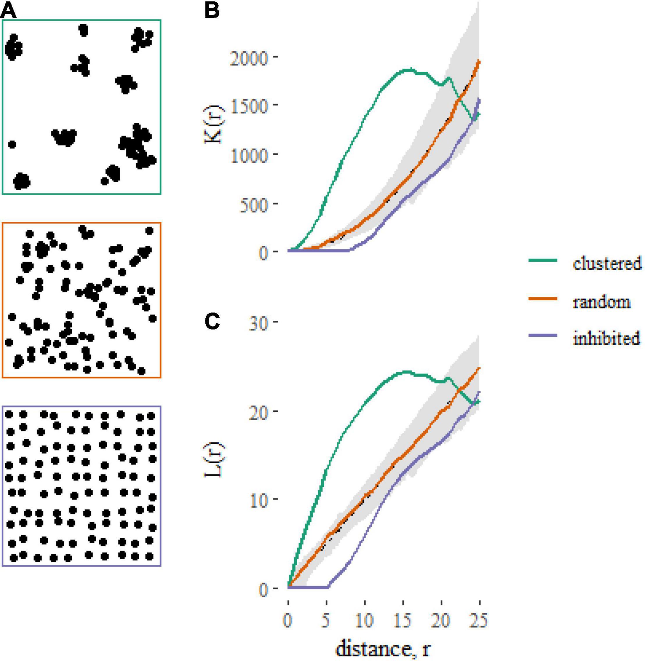
Figure 1. Examples of contrasting spatial point patterns (A) simulated on square, 100 × 100 unit plots, and their corresponding summary statistics (B: K-function, C: L-function). The gray shaded regions represent 95% simulation envelopes around the expected K-function [K(r) = πr2 ] or L-function [L(r) = r] under Complete Spatial Randomness (CSR). Clustered spatial point patterns, when points are closer together than expected under CSR, are indicated by K-functions greater than πr2 and L-functions greater than r. Inhibited patterns, when points are further apart than expected under CSR, are indicated by K-functions less than πr2 and L-functions less than r.
where I(.) is an indicator function that equals 1 when the distance between points dij is less or equal to r and is zero otherwise. The term eij is an edge correction function (Ripley, 1977; Diggle, 2003; Baddeley et al., 2015) that corrects for unobserved neighborhoods that lie beyond the edge of the study area. Note that throughout this tutorial we use a “border” edge correction, which takes the value 1 for focal individuals greater than a distance r from the edge and 0 otherwise (because only part of the neighborhoods of these individuals are inside the plot). With this correction, points within a distance r of the edge do not contribute to the estimate of K(r) as focal individuals. However, points that do not qualify as focal individuals are still included as neighbors (i.e., they can be part of the neighborhood of other focal individuals that are themselves greater than distance r from the plot boundary). When points are located homogeneously and independently, which can be considered the null hypothesis, the K-function takes the form K(r) = πr2.
Once the K-functions of the replicate point patterns have been computed, the models relate the values of K(r) at each distance (r) to the predictors, using separate linear models or linear-mixed effects models for each distance. At this stage, the models at each distance are independent of each other, except for sharing the same set of predictors. The dependence among distances is accounted for when calculating confidence intervals through bootstrapping (Bagchi and Illian, 2015). The outcome of the analysis is a set of functions that describe how each predictor affects the K-function at each distance (r). Positive values indicate that increasing values of the predictors are associated with increased clustering; negative values of the function indicate that increasing the predictor is associated with decreased clustering.
In the first section, we will present examples applied to simulated data sets of increasing complexity. In the second section, we will apply the methods to a data set available within the spatstat package (Baddeley and Turner, 2005): the Lansing plot data set.
Spatial point patterns usually include information about the locations of individuals (x, y coordinates). We simulate data on square plots, with each side one unit long (units here are arbitrary). In all simulations we generate 100 spatial point patterns (replicates), each with a different average density of points. Throughout this tutorial we will consider spatial point patterns generated from homogeneous point processes, which do not have gradients in average point densities. Code for simulating spatial point patterns is shown in Box 1.
Box 1. Generating spatial point patterns with spatstat (Baddeley and Turner, 2005) in R. We simulate a data set of 100 observations from two covariates (f, 100 discrete values sampled from two levels; x, 100 continuous values drawn from a uniform distribution), and a grouping variable, gr (by binning each sequence of 10 cases into one of 10 groups).
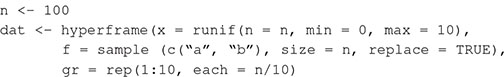
We simulate spatial points using functions in spatstat. The densities of points in the plots (plot dimensions are 1 unit × 1 unit) are randomly drawn from a uniform distribution between 20 and 100. The code returns a list of spatial point patterns, each of class ppp.
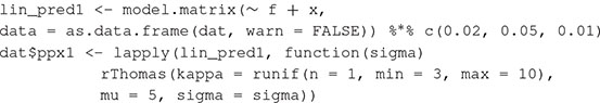
(a) Clustering varies with covariates: We can simulate clustered point patterns as realizations of a uniform Thomas cluster process (using the spatstat function rThomas). In the uniform Thomas cluster process, a set of “parent” points are generated from a poisson process with density σ. Offspring points are simulated around each parent point, with the number of offspring per parent drawn from a poisson distribution with mean σ, and the displacement of each offspring from its parent drawn from a normal distribution with mean 0 and standard deviation σ. The angle from parent to offspring is drawn from a uniform distribution between 0 and 180°. In this example, we make σ a linear function of the covariates where it is larger for f = “a” than f = “b” and increases with x (so group b and higher x is associated with less clustered points).
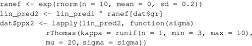
(b) Adding group effects:
We also allow σ to vary among groups by drawing a difference (from a normal distribution) between the mean σ and the σ in each group. Variation in σ among groups can be included by multiplying the linear predictor by a group specific number (σ must be positive, so the group-effect must be too).
A straightforward question to ask of a set of spatial point patterns might be what the average K-function is across the replicate patterns. For example, we might want to test whether red maple trees from multiple populations are generally clustered [i.e. K(r) > πr2] or inhibited [i.e. K(r) < πr2]. The mean K-function can be found by fitting an intercept-only model using the code
The function requires a formula with a point pattern object (class “ppp” from spatstat) as the response. The hyper argument specifies the hyperframe containing the data for the model. Example code in which data are converted into a ppp object and a hyperframe is provided in Box 2 and the Supplementary material. The user must specify the sequence of distances (r) at which K(r) should be modeled, the edge correction to be applied (correction), and the type of weights to be used in the model fitting (weights_type). The sequence of distances must begin at 0 and it is recommended that the maximum distance at which K(r) is estimated and modeled does not exceed ¼ the shortest plot dimension because estimates of K(r) at greater distances can be biased (Ripley, 1976). Edge corrections are defined by the spatstat package and we use the “border” correction here because it is fast and can be applied to plots of arbitrary shape. Other corrections, for example, Ripley’s isotropic correction (Ripley, 1976) are slower and have restrictions on plot dimensions but discard less information. These other edge corrections can be used in the RSPPlme4 package by specifying them instead of the “border” correction (e.g., correction =“isotropic”). The RSPPlme4 package offers various options for weights_type and a sensible default is to weight by the number of points in each replicate (nx; Diggle et al., 1991). Other options weight by the number of point pairs (nx2; Baddeley et al., 1993) or, when analyzing bivariate point patterns (the distribution of points of one type around another) the number or density of point pairs (nxny or nxny_A; Landau et al., 2004). For a fuller discussion of weighting options see Bagchi and Illian (2015).
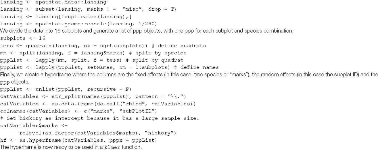
Box 2.Running a replicated spatial point pattern on spatstat.data::lansing. The lansing object maps the spatial distribution of five tree species in a single square plot, plus a sixth “misc” mark that we do not use. We drop data on this miscellaneous species and any duplicated plots below. We also rescale the plot to units of meters.
The Supplementary Information includes additional examples on point patterns created by artificially increasing or decreasing the clustering of trees from the Lansing data set.
It is worth pointing out one practical pitfall with fitting these models. Some edge corrections (e.g., the border correction) eliminate focal points that lie too near (specifically, <r) the edge of the plot. When point patterns with very few points are included in analyses, this process can lead to replicates with no pairs of points (<2 points), resulting in errors. To avoid this issue, the default settings on the model fitting functions internally filter out point patterns which have no pairs of points remaining after edge corrections and give warnings with the row numbers of the offending point patterns. Users who want more control can turn this feature off by setting remove_zero_weights = FALSE.
There are print and plot methods for the resulting R object, but these are rarely interpretable without some measure of uncertainty. The confidence interval around the model’s estimate of the K-function can be estimated with:
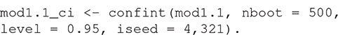
Confidence intervals are calculated using a semi-parametric bootstrapping approach (Landau and Everall, 2008; Bagchi and Illian, 2015). Note that the method estimates frequentist confidence intervals, not a simulation envelope (see Baddeley et al., 2014 for a discussion of the difference). The user must specify the number of bootstrap samples and can optionally specify the level of the confidence interval (the default is 95% confidence intervals as in this example). The random number seed can be set with the iseed argument to allow results to be reproducible.
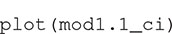
There are print and plot methods for the resulting object. For example,
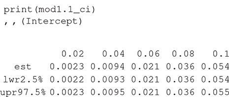
The numbers in the column headings provide the distances (r) at which K(r) is estimated, with the rows containing the estimates and confidence intervals. The object can be plotted with
The result is a ggplot2 object, allowing additional formatting using ggplot2 functions. For example, in Figure 2 we have formatted the plot, modified the y-axis label and added a curve with the expected K-function under complete spatial randomness (πr2 added to the plot as a dotted line using geom_function). The solid line shows the estimated mean K-function across the 100 point patterns. The confidence interval is represented with a gray shaded region, which is very narrow in this case. The confidence intervals will be wider, and hence more visible, in subsequent figures.
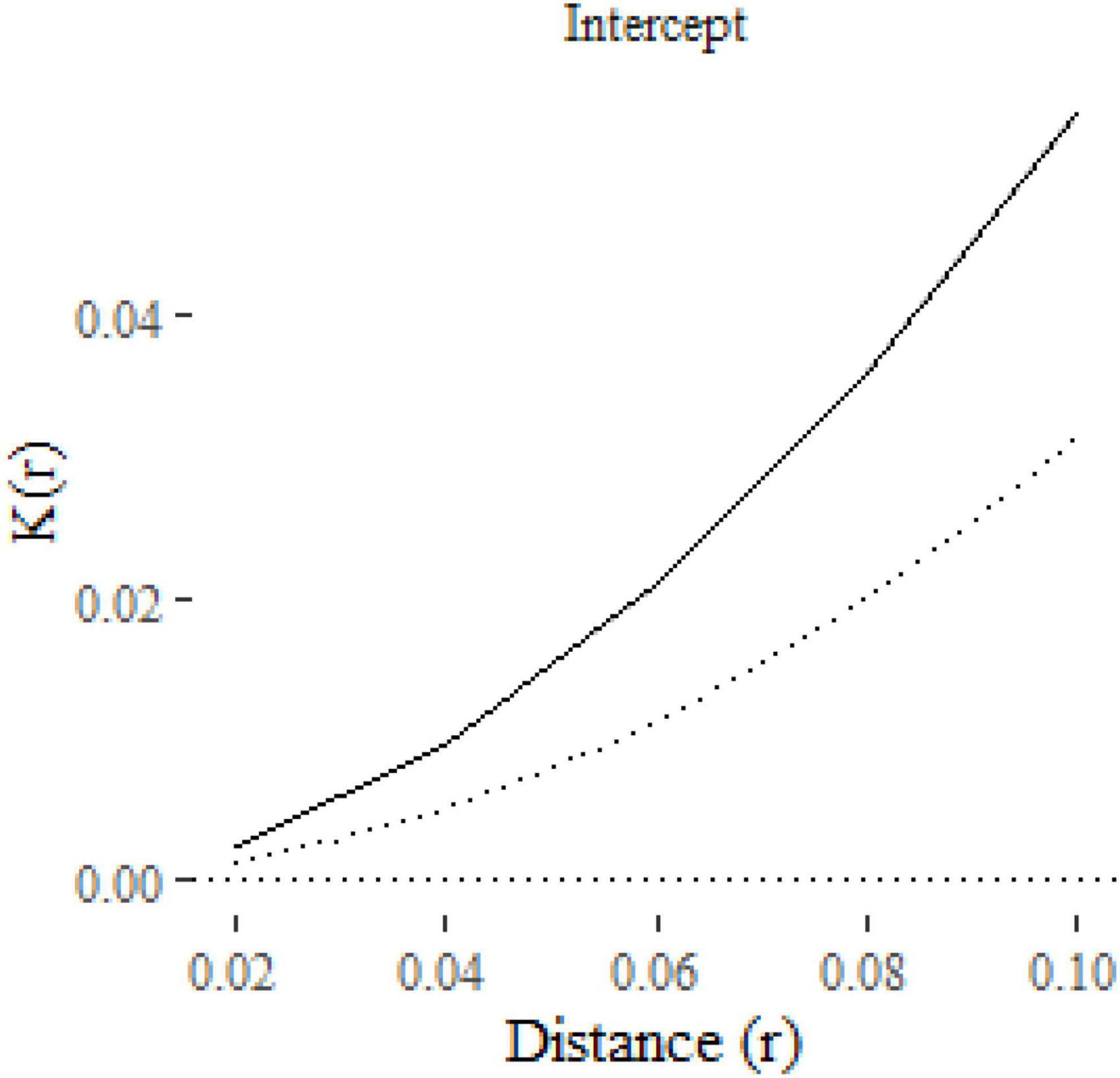
Figure 2. A plot of the K-function predicted by an intercept-only klm model fitted to 100 replicate point patterns. The dotted line is the expected K-function under complete spatial randomness. The gray shaded area around the solid line represents the 95% confidence interval.
The key value of the approach lies in the ability to link variation in spatial clustering to covariates of interest. Clustering in the simulated point patterns (see Box 1) was influenced by a discrete variable, f (where f = a had a smaller standard deviation, σ, than f = b) and a continuous variable x (σ increased with increasing x). Increasing the parameter σ increases the deviation of offspring points around the center of the cluster (the parent point), so lower σ (f = a and lower values of x) will be associated with increasingly clustered point patterns [i.e., K(r) will increase more rapidly over closer distances]. To quantify the effect of these covariates on K(r), we can fit the following model and compute and plot (Figure 3) confidence intervals for the coefficients with:
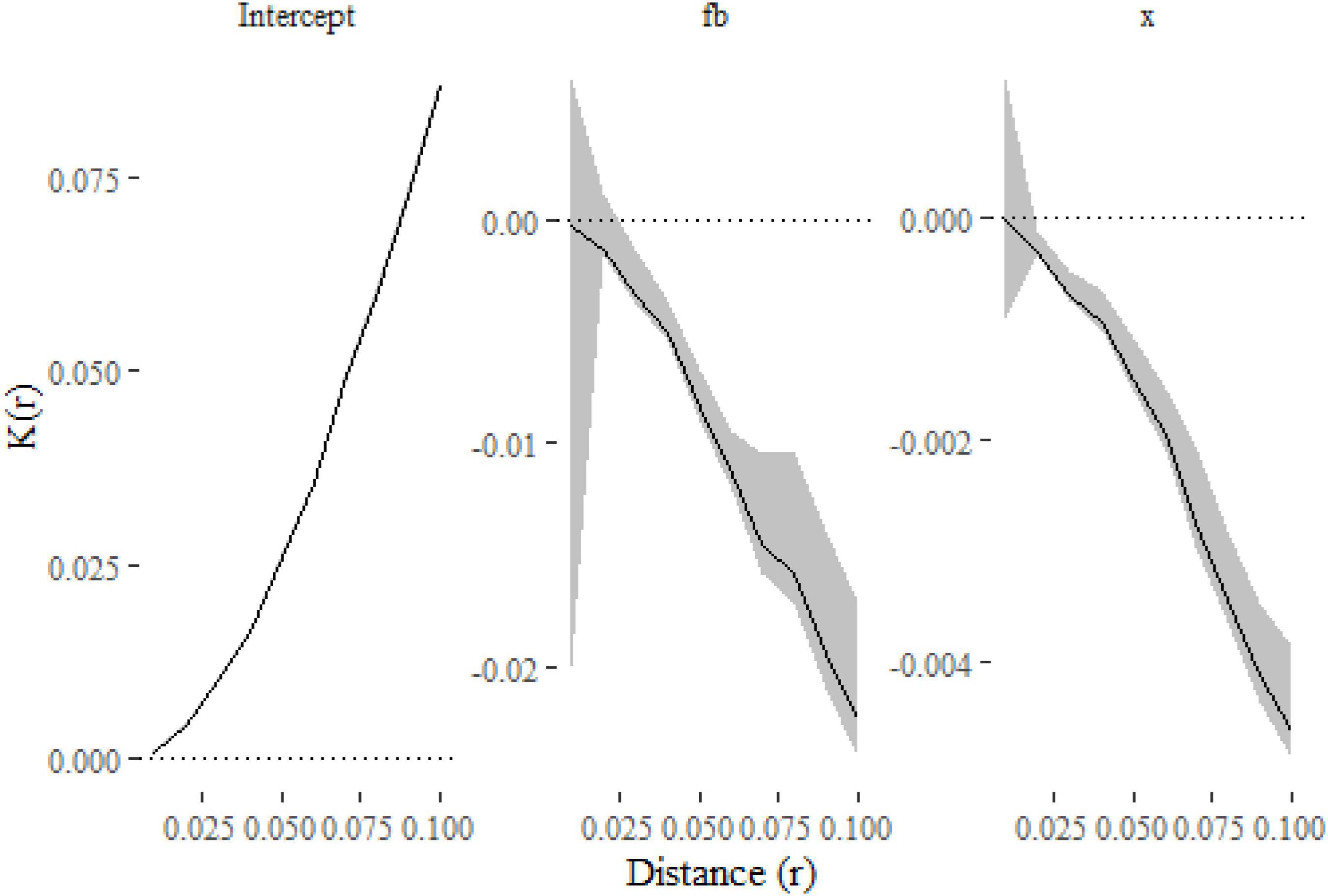
Figure 3. The parameter estimates from the models as functions of distance. The lines show the effect of each covariate on K estimated at a given distance, with 99% confidence intervals indicated with gray shading. The plots indicate that the K-function is decreased (and so points are less clustered) when f = b and as x increases.
The only substantial difference from the first model is the inclusion of f and x in the formula. We have also estimated (and modeled) K(r) at a finer resolution of distances and computed 99% confidence intervals in this example. Figure 3 shows that clustering is reduced when f = b and as x increases, which is consistent with the simulations where both terms widened the dispersal kernel around parent points.
It might also be useful to plot predictions from the model. For example, we might want to visually compare the K-functions for the different levels of f. The confint function includes a newdata argument that allows the user to specify covariate values for which predictions (and confidence intervals) are required. Code to get predictions at f = a and f = b at specific values of x (at x = 1, 5 and 10) is
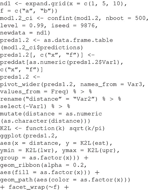
Which gives us Figure 4. Note the use of the transformation to rescale the y axis to plot an L-function rather than K-function [where, ]. The L-function is less visually dominated by larger distances than the K-function, which aids readability. We have added some further formatting for aesthetics and labeling.
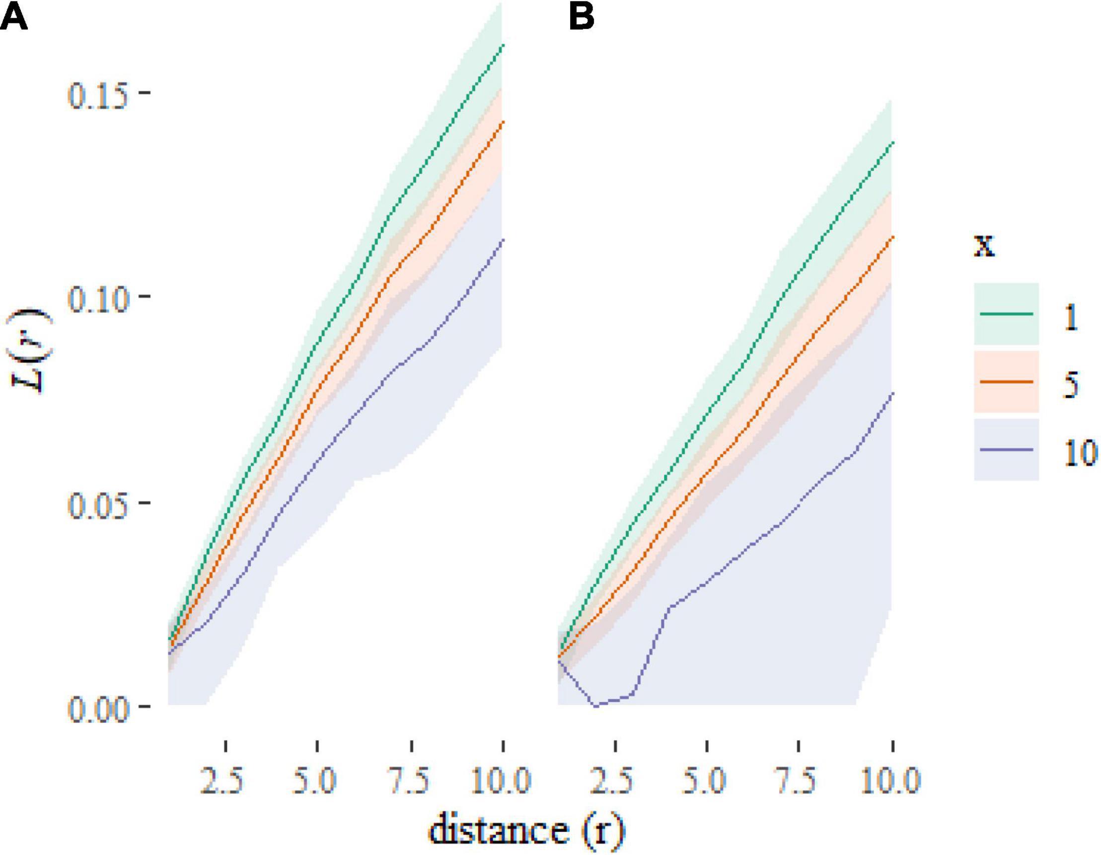
Figure 4. Plot of predictions at new combinations of covariate values. The plots show that the L-functions are predicted to be higher (more clustered) when f = a (A) than when f = b (B) and to decrease as x increases.
The analyses in the previous sections assumed that the replicate point patterns were independent of each other. Dependency among replicates can arise, for example, from proximity in space, time and genetic relatedness. If unaccounted for, dependence among replicates reduces estimates of uncertainty spuriously, leading to exaggerated confidence in parameter estimates and, as a consequence, inferences. Mixed-effects models (Pinheiro and Bates, 2000; Bolker et al., 2009) have become the standard approach for addressing dependence in linear models.
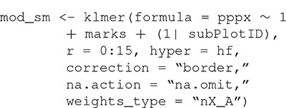
The second set of point patterns in the simulated data (ppx2), was influenced by group-level effects – specifically, the σ parameter was multiplied by a group-specific positive value. The group-level effects can be accounted for by fitting mixed-effects models of the K-functions using the klmer function.

The formula argument uses the syntax of the lme4 package (Bates et al., 2015). The rest of the arguments are identical to the klm function.
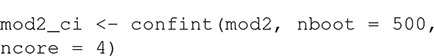
Confidence intervals can be calculated using confint, which has similar arguments to the equivalent function for klm. For simplicity, we have dropped the level argument, which means the default 95% confidence intervals will be estimated. One difference is the capacity of the confint function for klmer objects to use parallel computation (by specifying ncore > 1). Parallelization of the bootstrapping is very helpful because the process can be quite time consuming with large datasets.
Once the confidence intervals have been computed they can easily be printed or plotted. For example, with
The negative effect of both f = b and x on clustering is once again apparent (Figure 5).
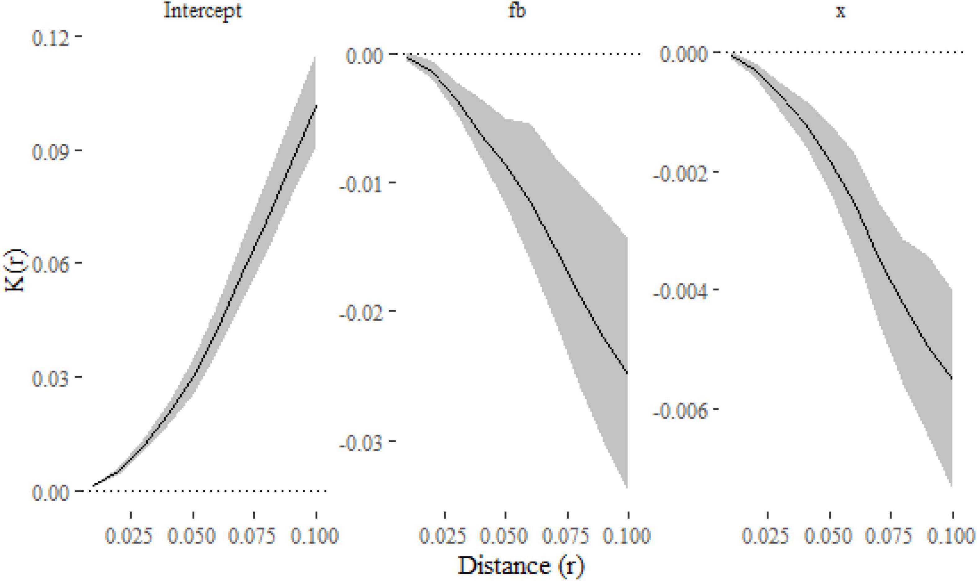
Figure 5. Parameter estimates and their confidence intervals for simulated replicated spatial point patterns calculated using the klmer and confint functions. Estimates for both f = b and x are negative, which indicate that they have a negative effect of spatial clustering.
We use a dataset on spatial distributions of five tree species in Lansing Woods, MI, United States (Gerrard, 1969) as an example of how replicated point pattern analysis can be applied to observed data. The Lansing dataset contains information on locations of trees on a 19.6 acre square plot with the species identification of each individual associated with its point as a mark (i.e., the dataset is a marked point pattern). The original data set is not a replicated point pattern, so we split it into subplots to demonstrate the technique. Such splitting of continuous data into replicate patterns has some advantages (e.g., it allows the user to generate confidence intervals), but care is needed to satisfy the assumption that the subplots are independent of each other (e.g., subplots are sampled to be separated by at least some minimum distance) Box 2 provides details on how the data were arranged into the correct structure to enable analysis.
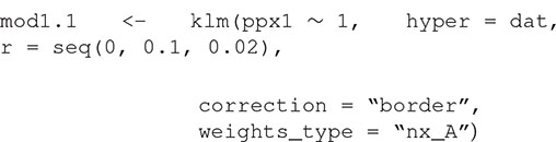
Once the dataset is prepared, we fit the model with the klmer function.
We can make predictions of the K-function for each species and calculate the confidence intervals around the parameter estimates (Figure 6) and predictions (Figure 7).
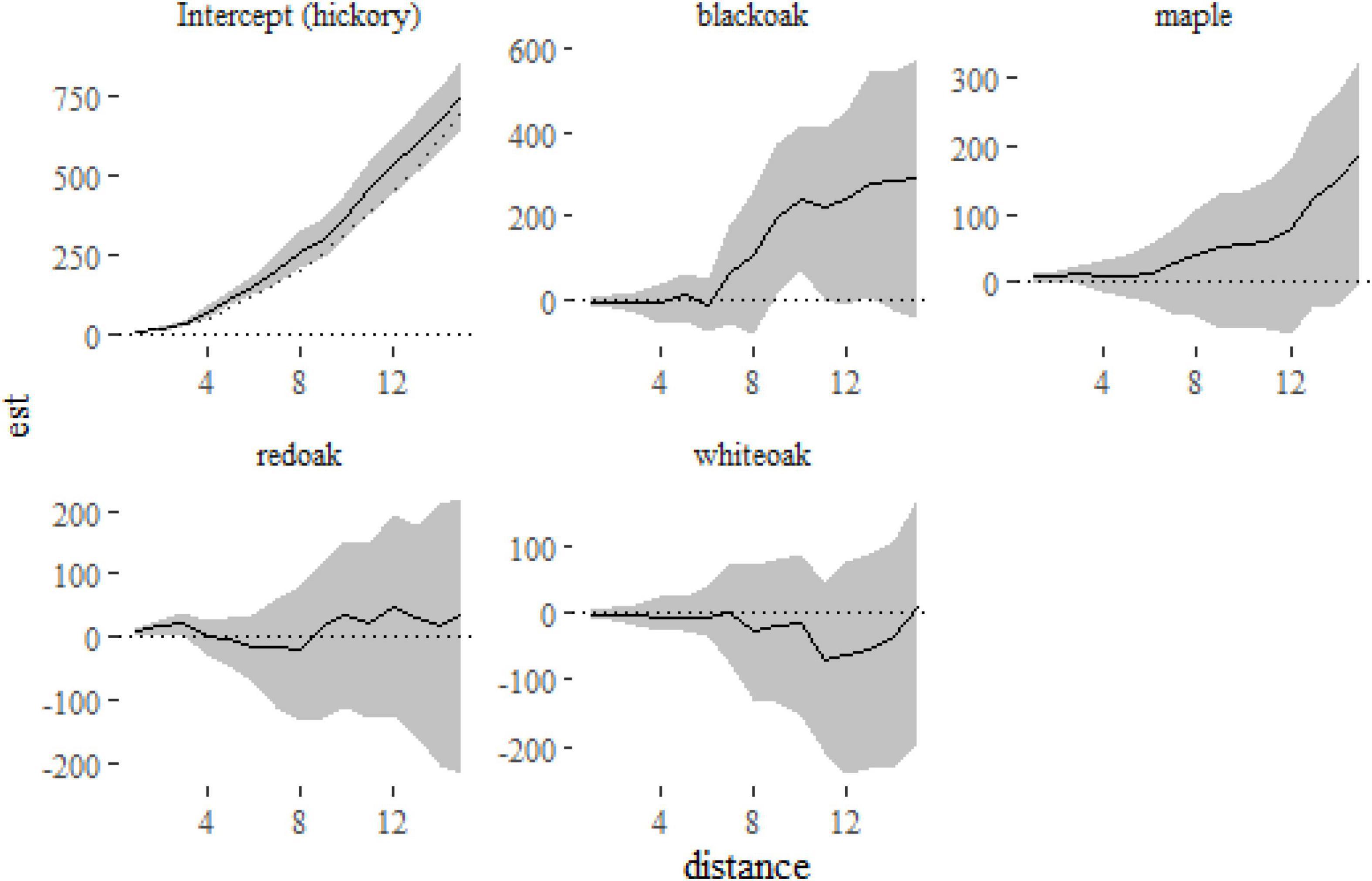
Figure 6. Fixed-effect estimates from the klmer model fitted to the Lansing data set. The intercept term (hickory) shows a small amount of clustering relative to the expectation under complete spatial randomness πr2 (indicated on the first panel with a dotted line). The other panels show the differences between the K-function for each of the other species and hickory.
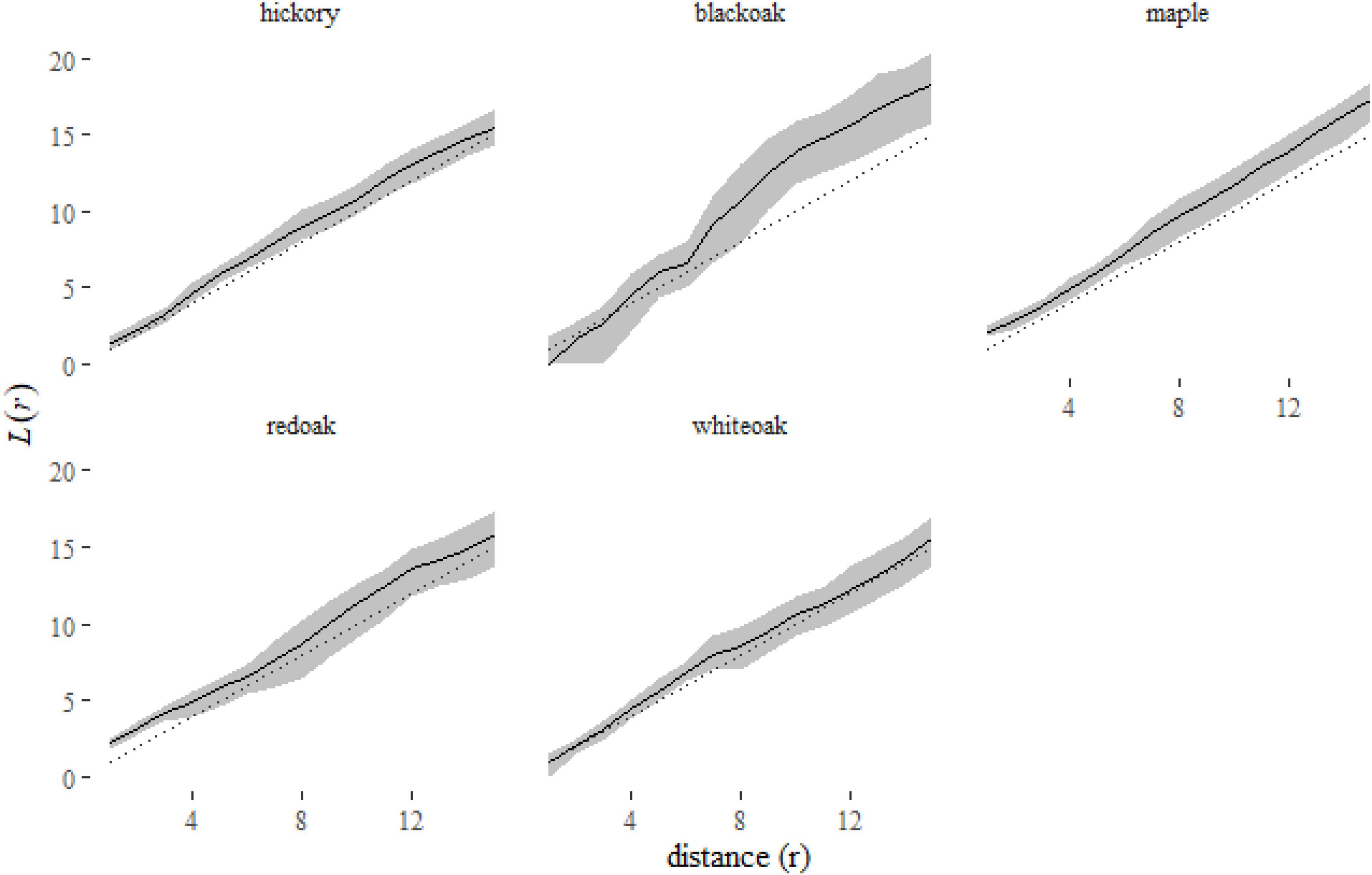
Figure 7. A plot of the predictions from the klmer model for each species in the Lansing data set. Here we have plotted the corresponding L-functions, a rescaling of the K-function [ )]. Using this rescaled statistic, it is easier to see the deviations of species distributions from the expectation under complete spatial randomness [dotted line, L(r) = r].
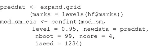
The resulting parameter estimates and confidence intervals can be plotted using plot(mod_sm_cis). Alternatively, they can be converted into a plot-ready tibble using the function makePlotData_klmerci, and formatted further by the user (see Supplementary Information).
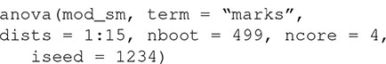
From Figure 6 we can see that hickory, the reference level in the model, is slightly more clustered than that expected under complete spatial randomness. The other panels show the difference between each species and hickory, suggesting little difference between the species (although black oak is marginally more clustered at distances > 8 m). A formal test of differences among species can be run with
Which gives us
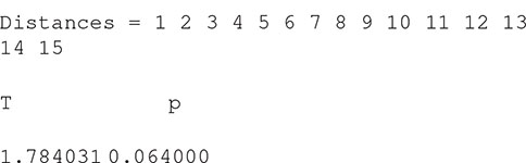
And confirms that the differences among species are, marginally, not significant. It is possible to specify alternative distance ranges, although any choice should be made a priori (Loosmore and Ford, 2006; Baddeley et al., 2014).
A plot of the predictions of the L-function of each species (Figure 7) shows us that some species, like black oak and maple, are consistently clustered [L(r) > r]. No species is consistently inhibited [L(r) < r]. Red oak and white oak indicate some clustering at short distances (r < 6 meters).
Spatial patterns offer insight into many ecological questions. Although ecologists have access to a wide variety of methods to analyze spatial point patterns (Wiegand and Moloney, 2004; Law et al., 2009), few of the available methods explicitly deal with replication. Statistical techniques for analyzing RSPP have existed in the statistical literature for some time (Diggle et al., 1991, 2000; Baddeley et al., 1993; Landau and Everall, 2008), but have been used sparingly in ecological applications (but see Riginos et al., 2005; Bagchi and Illian, 2015; Ramón et al., 2016; Bagchi et al., 2018). We believe that the paucity of RSPP analyses in the ecological literature is partly due to a lack of software. Filling that gap is our goal in this article. We introduce the RSPPlme4 package in the R programming language with worked examples of analyses with and without random effects.
It is worth considering how the RSPP methods we present might simplify the job of interrogating spatial point patterns for information about ecological patterns and processes. Analyses of spatial point patterns in ecology have generally taken a null model testing approach, where an observed summary statistic is compared to distribution of that statistic generated under a null model (Condit et al., 2000; Getzin et al., 2008; Bagchi et al., 2011). The null model approach is very flexible because computer simulations can be customized to capture complex aspects of the data generation process (Wiegand and Moloney, 2004). However, the null-model workflow requires a reasonable level of programming expertise, and also encourages a null hypothesis testing approach that is frequently criticized (e.g., McShane et al., 2019). Alternative null models often require substantial changes to the underlying code, which can require additional programming and run time. Null models also require greater complexity to account for uncertainty in estimates of the summary statistics and variation among samples.
The RSPP modeling method, in contrast, takes a parameter estimation approach, which is increasingly familiar to ecologists. Parameter estimates can be used for hypothesis testing (e.g., checking if confidence intervals overlap zero), but also allow more nuanced inference about how a unit increase in a predictor alters the spatial structure of the population. Variation among samples and groups is explicitly estimated, and this variation can be informative in its own right (Gelman and Hill, 2006). Once the data are formatted appropriately, the complexity of code for fitting models is comparable to fitting generalized linear models. The user needs to make decisions about the appropriate distance range, edge correction, and weights type, but specifying those options is straightforward. The fact that parameter estimates and predictions are functions rather than single scalar numbers and summary statistics are outcomes of, rather than inputs to, the data generation process, makes interpretation harder. These complicating features of the RSPP analysis methods described here, however, are shared with null model approaches (Loosmore and Ford, 2006; Baddeley et al., 2014). There is a trade-off between the flexibility of the null model approach to specify details of the data generation process and the ease of using the familiar linear model framework to quickly specify a large range of possible relationships. Ultimately, the combination of both methods provides greater flexibility for researchers to address questions about the spatial structure of populations.
There are a variety of ways in which the methods we outline here could be extended further. We have limited our discussion to homogeneous point processes, where the mean density of points is constant over the study area. The approach can be extended to inhomogeneous point processes, where point densities vary along gradients by using inhomogeneous K-functions in the models (Baddeley et al., 2000, 2015; Diggle et al., 2007). One potential complication in expanding to inhomogeneous patterns is that the local density for computing the inhomogeneous K-function generally has to be estimated from the same data, which can result in very low power (Baddeley et al., 2014). A second extension of the approach would be to allow for more complex correlation structures among replicates. The inclusion of random effects helps account for the dependence among replicates in the same group, but does not allow for a continuous gradation of the dependency among individuals. For example, the correlation in the responses between replicates might decrease with the time between observations, as might be captured by a continuous auto-regressive model (Pinheiro and Bates, 2000). Third, we do not explicitly consider analyses of marked point processes, although marks (information on individual points) can be used to divide the point pattern into replicates (see the analyses of the Lansing data set). Finally, the software in RSPPlme4 (version 0.2.0) used in this tutorial is still in an early stage of development, so testing, identifying and removing bugs, and expanding the functionality and usability of the package are important tasks for the near future.
In this article, we have tried to demonstrate that the process of fitting models to RSPP data can be relatively straightforward. There is still much that we do not know about the spatial structures of populations and communities, the processes that generate them and how they vary with traits, ontogeny and environmental context. It is our hope that introducing these methods for RSPP analysis will accelerate our progress towards filling these gaps in our understanding.
The original contributions presented in the study are included in the article/Supplementary Material. Code used in this paper is available from GitHub BagchiLab-Uconn/RSPP_Example, 10.5281/zenodo.6447942. Further inquiries can be directed to the corresponding author.
RB, ML, VM, and DD developed the idea. RB and ML did the analysis with input from VM and DD. RB drafted the manuscript with input from all other authors. All authors contributed to the article and approved the submitted version.
This project received funding from the European Union’s Seventh Framework Program for Research, Technological Development and Demonstration under grant agreement no. GA-2010-267243 – PLANT FELLOWS.
The authors declare that the research was conducted in the absence of any commercial or financial relationships that could be construed as a potential conflict of interest.
All claims expressed in this article are solely those of the authors and do not necessarily represent those of their affiliated organizations, or those of the publisher, the editors and the reviewers. Any product that may be evaluated in this article, or claim that may be made by its manufacturer, is not guaranteed or endorsed by the publisher.
The Supplementary Material for this article can be found online at: https://www.frontiersin.org/articles/10.3389/ffgc.2022.810010/full#supplementary-material
Augspurger, C. K. (1986). Morphology and dispersal potential of wind-dispersed diaspores of neotropical trees. Am. J. Bot. 73, 353–363. doi: 10.1002/j.1537-2197.1986.tb12048.x
Baddeley, A., Diggle, P. J., Hardegen, A., Lawrence, T., Milne, R. K., and Nair, G. (2014). On tests of spatial pattern based on simulation envelopes. Ecol. Monogr. 84, 477–489. doi: 10.1890/13-2042.1
Baddeley, A., Rubak, E., and Turner, R. (2015). Spatial Point Patterns: Methodology and Applications with R (Chapman & Hall/CRC Interdisciplinary Statistics). 1st ed. Boca Raton: Chapman and Hall/CRC.
Baddeley, A., and Turner, R. (2005). spatstat paanr package for analyzing spatial point patterns. J. Stat. Softw. 12, 1–42. doi: 10.18637/jss.v012.i06
Baddeley, A. J., Moller, J., and Waagepetersen, R. (2000). Non- and semi-parametric estimation of interaction in inhomogeneous point patterns. Stat. Neerl. 54, 329–350. doi: 10.1111/1467-9574.00144
Baddeley, A. J., Moyeed, R. A., Howard, C. V., and Boyde, A. (1993). Analysis of a Three-Dimensional Point Pattern with Replication. Appl. Stat. 42:641. doi: 10.2307/2986181
Bagchi, R. (2020). RSPPlme4: Analysis of replicated point patterns with “lme4”. Switzerland: Zenodo. doi: 10.5281/zenodo.3829093
Bagchi, R., Henrys, P. A., Brown, P. E., Burslem, D. F. R. P., Diggle, P. J., Gunatilleke, C. V. S., et al. (2011). Spatial patterns reveal negative density dependence and habitat associations in tropical trees. Ecology 92, 1723–1729. doi: 10.1890/11-0335.1
Bagchi, R., and Illian, J. B. (2015). A method for analysing replicated point patterns in ecology. Methods Ecol. Evol. 6, 482–490. doi: 10.1111/2041-210X.12335
Bagchi, R., Swamy, V., Latorre Farfan, J.-P., Terborgh, J., Vela, C. I. A., Pitman, N. C. A., et al. (2018). Defaunation increases the spatial clustering of lowland Western Amazonian tree communities. J. Ecol. 106, 1470–1482. doi: 10.1111/1365-2745.12929
Bates, D., Mächler, M., Bolker, B., and Walker, S. (2015). Fitting linear mixed-effects models using lme4. J. Stat. Softw. 67, 1–48. doi: 10.18637/jss.v067.i01
Bolker, B., and Pacala, S. W. (1997). Using moment equations to understand stochastically driven spatial pattern formation in ecological systems. Theor. Popul. Biol. 52, 179–197. doi: 10.1006/tpbi.1997.1331
Bolker, B. M., Brooks, M. E., Clark, C. J., Geange, S. W., Poulsen, J. R., Stevens, M. H. H., et al. (2009). Generalized linear mixed models: a practical guide for ecology and evolution. Trends Ecol. Evol. 24, 127–135. doi: 10.1016/j.tree.2008.10.008
Condit, R., Ashton, P. S., Baker, P., Bunyavejchewin, S., Gunatilleke, S., Gunatilleke, N., et al. (2000). Spatial patterns in the distribution of tropical tree species. Science 288, 1414–1418. doi: 10.1126/science.288.5470.1414
Diggle, P. (2003). Statistical Analysis of Spatial Point Patterns. 2nd. illustrated ed. London: Arnold.
Diggle, P. J., Gómez-Rubio, V., Brown, P. E., Chetwynd, A. G., and Gooding, S. (2007). Second-order analysis of inhomogeneous spatial point processes using case-control data. Biometrics 63, 550–557. doi: 10.1111/j.1541-0420.2006.00683.x
Diggle, P. J., Lange, N., and Beneš, F. M. (1991). Analysis of variance for replicated spatial point patterns in clinical neuroanatomy. J. Am. Stat. Assoc. 86, 618–625. doi: 10.1080/01621459.1991.10475087
Diggle, P. J., Mateu, J., and Clough, H. E. (2000). A comparison between parametric and non-parametric approaches to the analysis of replicated spatial point patterns. Adv. Appl. Probab. 32, 331–343. doi: 10.1239/aap/1013540166
Gelman, A., and Hill, J. (2006). Data Analysis Using Regression and Multilevel/Hierarchical Models. 1st ed. Cambridge: Cambridge University Press.
Gerrard, D. J. (1969). Competition quotient: a new measure of the competition affecting individual forest trees Research Bulletin 20. Agricultural Experiment Station: Michigan State University.
Getzin, S., Wiegand, T., Wiegand, K., and He, F. (2008). Heterogeneity influences spatial patterns and demographics in forest stands. J. Ecol. 96, 807–820. doi: 10.1111/j.1365-2745.2008.01377.x
Illian, J., Penttinen, A., Stoyan, H., and Stoyan, D. (2007). Statistical Analysis and Modelling of Spatial Point Patterns. Chichester, UK: John Wiley & Sons, Ltd, doi: 10.1002/9780470725160
Landau, S., and Everall, I. P. (2008). Nonparametric bootstrap for k-functions arising from mixed-effects models with applications in neuropathology. Stat. Sin. 18, 1375–1393.
Landau, S., Rabe-Hesketh, S., and Everall, I. P. (2004). Nonparametric One-way Analysis of Variance of Replicated Bivariate Spatial Point Patterns. Biom. J. 46, 19–34. doi: 10.1002/bimj.200310010
Law, R., and Dieckmann, U. (2000). A Dynamical System for Neighborhoods in Plant Communities. Ecology 81:2137. doi: 10.2307/177102
Law, R., Illian, J., Burslem, D. F. R. P., Gratzer, G., Gunatilleke, C. V. S., and Gunatilleke, I. A. U. N. (2009). Ecological information from spatial patterns of plants: insights from point process theory. J. Ecol. 97, 616–628. doi: 10.1111/j.1365-2745.2009.01510.x
Loosmore, N. B., and Ford, E. D. (2006). Statistical inference using the g or K point pattern spatial statistics. Ecology 87, 1925–1931. doi: 10.1890/0012-9658(2006)87[1925:siutgo]2.0.co;2
McShane, B. B., Gal, D., Gelman, A., Robert, C., and Tackett, J. L. (2019). Abandon Statistical Significance. Am. Stat. 73, 235–245. doi: 10.1080/00031305.2018.1527253
Murrell, D. J., and Law, R. (2002). Heteromyopia and the spatial coexistence of similar competitors. Ecol. Lett. 6, 48–59. doi: 10.1046/j.1461-0248.2003.00397.x
Pinheiro, J., and Bates, D. (2000). Mixed-Effects Models in S and S-PLUS. 1st ed. Berlin: Springer Nature.
Ramón, P., de la Cruz, M., Chacón-Labella, J., and Escudero, A. (2016). A new non-parametric method for analyzing replicated point patterns in ecology. Ecography 39, 1109–1117. doi: 10.1111/ecog.01848
Riginos, C., Milton, S. J., and Wiegand, T. (2005). Context-dependent interactions between adult shrubs and seedlings in a semi-arid shrubland. J. Veg. Sci. 16, 331–340. doi: 10.1111/j.1654-1103.2005.tb02371.x
Ripley, B. D. (1976). The second-order analysis of stationary point processes. J. Appl. Probab. 13, 255–266. doi: 10.2307/3212829
Ripley, B. D. (1977). Modelling Spatial Patterns. J. R. Stat. Soc. Ser. B 39, 172–192. doi: 10.1111/j.2517-6161.1977.tb01615.x
Seidler, T. G., and Plotkin, J. B. (2006). Seed dispersal and spatial pattern in tropical trees. PLoS Biol. 4:e344. doi: 10.1371/journal.pbio.0040344
Smith, J. R., Bagchi, R., Ellens, J., Kettle, C. J., Burslem, D. F. R. P., Maycock, C. R., et al. (2015). Predicting dispersal of auto-gyrating fruit in tropical trees: a case study from the Dipterocarpaceae. Ecol. Evol. 5, 1794–1801. doi: 10.1002/ece3.1469
ter Steege, H., Pitman, N. C. A., Sabatier, D., Baraloto, C., Salomão, R. P., Guevara, J. E., et al. (2013). Hyperdominance in the Amazonian tree flora. Science 342:1243092. doi: 10.1126/science.1243092
Wickham, H., Averick, M., Bryan, J., Chang, W., McGowan, L., François, R., et al. (2019). Welcome to the tidyverse. JOSS 4:1686. doi: 10.21105/joss.01686
Wiegand, T., and Moloney, K. A. (2004). Rings, circles, and null-models for point pattern analysis in ecology. Oikos 104, 209–229. doi: 10.1111/j.0030-1299.2004.12497.x
Wiegand, T., and Moloney, K. A. (2010). Handbook Of Spatial Point-pattern Analysis In Ecology (chapman & Hall/crc Applied Environmental Statistics). 1st ed. Boca Raton: Chapman And Hall/CRC.
Keywords: K-function, spatial structure, mixed-effects model (MEM), R, ecological statistics, replication
Citation: Bagchi R, LaScaleia MC, Milici VR and Dalui D (2022) Replicated Spatial Point Pattern Analyses for Ecological Inference: A Tutorial Using the RSPPlme4 Package in R. Front. For. Glob. Change 5:810010. doi: 10.3389/ffgc.2022.810010
Received: 05 November 2021; Accepted: 29 March 2022;
Published: 29 April 2022.
Edited by:
Radim Matula, Czech University of Life Sciences Prague, CzechiaReviewed by:
Daniel J. Johnson, University of Florida, United StatesCopyright © 2022 Bagchi, LaScaleia, Milici and Dalui. This is an open-access article distributed under the terms of the Creative Commons Attribution License (CC BY). The use, distribution or reproduction in other forums is permitted, provided the original author(s) and the copyright owner(s) are credited and that the original publication in this journal is cited, in accordance with accepted academic practice. No use, distribution or reproduction is permitted which does not comply with these terms.
*Correspondence: Robert Bagchi, cm9iZXJ0LmJhZ2NoaUB1Y29ubi5lZHU=
Disclaimer: All claims expressed in this article are solely those of the authors and do not necessarily represent those of their affiliated organizations, or those of the publisher, the editors and the reviewers. Any product that may be evaluated in this article or claim that may be made by its manufacturer is not guaranteed or endorsed by the publisher.
Research integrity at Frontiers
Learn more about the work of our research integrity team to safeguard the quality of each article we publish.