Small Area Estimates for National Applications: A Database to Dashboard Strategy Using FIESTA

This paper demonstrates a process for translating a database of forest measurements to interactive dashboards through which users can access statistically defensible estimates and analyses anywhere in the conterminous US. It taps the extensive Forest Inventory and Analysis (FIA) plot network along with national remotely sensed data layers to produce estimates using widely accepted model-assisted and small area estimation methodologies. It leverages a decade’s worth of statistical and computational research on FIA’s flexible estimation engine, FIESTA, and provides a vehicle through which scientists and analysts can share their own tools and analytical processes. This project illustrates one pathway to moving statistical research into operational inventory processes, and makes many model-assisted and small area estimators accessible to the FIA community. To demonstrate the process, continental United States (CONUS)-wide model-assisted and small area estimates are produced for ecosubsections, counties, and level 5 watersheds (HUC 10) and made publicly available through R Shiny dashboards. Target parameters include biomass, basal area, board foot volume, proportion of forest land, cubic foot volume, and live trees per acre. Estimators demonstrated here include: the simplest direct estimator (Horvitz–Thompson), model-assisted estimators (post-stratified, generalized regression estimator, and modified generalized regression estimators), and small area estimators (empirical best linear unbiased predictors and hierarchical Bayes both at the area- and unit-level). Auxiliary data considered in the model-assisted and small area estimators included maps of tree canopy, tree classification, and climatic variables. Estimates for small domain sets were generated nationally within a few hours. Exploring results across estimators and target variables revealed the progressive gains in precision using (in order of least gain to highest gain) Horvitz–Thompson, post-stratification, modified generalized regression estimators, generalized regression estimators, area-level small area models, and unit-level small area models. Substantive gains are realized by expanding model-assisted estimators beyond post-stratification, allowing FIA to continue to take advantage of design-based inference in many cases. Caution is warranted in the use of unit-level small area models due to model mis-specification. The dataset of estimates available through the dashboards provides the opportunity for others to compare estimators and explore precision expectations over specific domains and geographic regions. The dashboards also provide a forum for future development and analyses.

Introduction

The USDA Forest Service, Forest Inventory and Analysis (FIA) program is responsible for reporting status and trends of the nation’s forests and is mandated by Congress, through the 1928 McSweeney-McNary Forest Research Act and the 1974 Forest and Rangeland Renewable Resources Planning Act, to inventory and maintain a national database and provide estimates at State and National levels. The inventory was designed to provide strategic level information (Gillespie, 1999), with states being the standard reporting units, and post-stratification being the predominant estimator used in production processes (Bechtold and Patterson, 2015). Yet, there is a growing need for more precise and statistically defensible estimates to support forest land management over sub-State areas (U.S. Department of Agriculture, 2014; Prisley et al., 2021; Wiener et al., 2021).

To provide some examples, while standard FIA reporting provides analyses over entire states or regional collections of counties within a state (Witt et al., 2018; U.S. Department of Agriculture, Forest Service, 2021), estimates of forest resources are frequently needed by individual counties for county-level assessments (Morin et al., 2015; Filippelli et al., 2020) and alignment of sustainable management practices to national efforts (U.S. Department of Agriculture, Forest Service, 2020). Further, the USDA Forest Service has emphasized an ecological approach to managing forests and directing policy by its development of a hierarchical framework of Ecological Units (ECOMAP; Cleland et al., 2007). The classification was aimed at providing a scientific basis for analyzing ecosystems at different scales, depending on the management need. The ECOMAP delineations are frequently used for analyzing vegetation patterns (West et al., 1998; Hanberry et al., 2018; Miller et al., 2018) and ecological subsections provide a national collection of areas for which estimates of forest attributes would be useful. As another example, the Forest Service has recognized the need for assessing and monitoring the hydrologic systems across the US. Quantifying forest attributes within watersheds, particularly in conjunction with disturbance events, is needed for assessing variables such as stream flow and snowpack (Goeking and Tarboton, 2020). It is important to have the ability to construct estimates of forest attributes across smaller political, ecological, and hydrologic areas of interest.

One question that frequently arises is: how can we take advantage of FIA’s extensive, strategic-level national database to generate estimates for areas that do not have enough sample plots using current estimation strategies to get meaningful estimates? Auxiliary data generated from remotely sensed platforms is abundant, inexpensive, and is often correlated with forest attributes of interest. One way to use the auxiliary data is to build a model for the forest attribute of interest using the FIA plot data as the response, and the auxiliary data intersected at those ground plots as the predictor variables. From this model, a wall-to-wall map of predictions of the forest attribute of interest is generated. The assumed statistical framework determines how the predicted values are aggregated to form an estimate and how the estimator accounts for the sampling design. Post-stratification is one of the simplest forms of model-assisted estimation and is the estimator currently employed in FIA’s production processes. But numerous other model-assisted estimators offer further opportunity to make better use of auxiliary data (e.g., McConville et al., 2020). In model-assisted estimation, the model is simply used as a vehicle for estimating parameters in the regression estimator formula. We are not making the assumption that the population was really generated by that model. Therefore, model-assisted estimators are considered robust to model mis-specification (meaning they are asymptotically unbiased for the population attribute and the variance formulas are valid) regardless of whether or not the working model is an accurate reflection of the relationship between the variable of interest and auxiliary variables. Small area estimators (e.g., Rao and Molina, 2015), on the other hand, are needed in instances where there are too few sample plots in order to produce a reliable estimate using only data within those small domains of interest. In this case, small area estimators “borrow strength” (both sample plots and auxiliary data) from other similar areas to increase the effective sample size from which information can be produced. This borrowing process is orchestrated through a model from which measures of precision can be derived. Small area estimators rely on model-based inference which means the observations are assumed to be random realizations of some superpopulation. That is, unlike model-assisted estimators (which rely on design-based inference), we are making the assumption that the model did generate the population. One should be careful when comparing the standard error estimates of design-based and model-based methods because each paradigm conceptualizes randomness differently. In design-based inference the primary source of randomness comes from the sampling of units from the population while model-based inference considers the data to be realizations from a superpopulation model. These different conceptualizations impact how the standard error of the estimator is calculated. In addition, substantial gains in precision can be realized from model-based estimators, but they can easily yield biased estimates if the model is mis-specified.

Recent reviews of the use of model-assisted and small area estimators in forest inventory applications are provided by Guldin (2021) and Dettmann et al. (2022). Extending beyond those reviews, the last year has seen a spike in investigations into improving precision in FIA estimates over small domains. For example, in the Interior Western US, estimates for multiple forest attributes were explored using a modified generalized regression estimator over counties (Wojcik et al., 2022). And area-level Hierarchical Bayesian and Empirical Best Linear Unbiased Predictor strategies were compared to post-stratification over ecological subsections (White et al., 2021). In the Pacific Northwest, Bell et al. (2022) compare Horvitz Thompson, generalized regression, and k-nearest neighbor synthetic estimates of aboveground live carbon. Temesgen et al. (2021) use Fay–Herriot models of above ground biomass and volume specific to stand-level inventories where variable radius plot locations may be unknown. In the Southern US, Cao et al. (2022) improve precision in volume estimates for counties using spatial area-level small area estimators. In the northern US, Harris et al. (2021) compare design- and model-based estimates in support of the National Woodland Owner Survey. Across the Western US, Gaines and Affleck (2021) estimate postfire tree density through temporal borrowing strategies. And across the conterminous US, Stanke et al. (2022) use rFIA to facilitate spatial Fay–Herriot models of forest carbon stocks.

Constructing estimates over non-traditional boundaries requires a shift to using these statistical estimators that can better leverage improved auxiliary remotely sensed data. FIESTA (Forest Inventory ESTimation for Analysis) (Frescino et al., 2020) is an R package that was originally developed to support the production of estimates consistent with current tools available from the FIA National Program, such as DATIM (Design and Analysis Toolkit for Inventory and Monitoring) and EVALIDator¹. FIESTA provides an alternative data retrieval and reporting tool that is functional within the R environment, allowing customized applications and compatibility with other R-based analyses. It hosts a growing suite of model-assisted and small area estimators. While the package itself is available publicly for R users, most forest land managers need tools that do not require programming expertise. A first step in making estimates available is through distribution via a dashboard.

In this paper we first demonstrate a national, production-level process whereby a large collection of model-assisted and small area estimators can be rapidly applied in FIESTA for a variety of forest attributes and domains across the conterminous US. Second, we compare the levels of precision that can be achieved using these different estimators for different sized domains, providing benchmarks from which future improvement can be made. And third, we provide estimates and their standard errors through publicly available dashboards so others can perform analyses in different regions of the country.

Materials and Methods

FIESTA

FIESTA is an R package made up of a set of functions for compiling response data and auxiliary information for use in different estimation strategies, including simple random sampling, model-assisted, and model-based small area estimation (SAE). The functions are categorized based on different purposes: FIESTA’s core functions include code for querying and summarizing FIA data and different types of spatial data; FIESTA modules present different estimation strategies; and FIESTA analysis functions are wrapper functions to streamline different estimation routines.

We created an analysis function to generate and compare estimates using several different estimators for any defined domain(s) as depicted in Figure 1. The analysis function combines FIESTA core functions to: (1) extract FIA inventory data and (2) compile and summarize auxiliary information from multiple spatial data layers by domain. These are shaded in blue to indicate data compilation processes. From here, another function formats the output from these core functions, for input to the FIESTA Green-Book (GB), Model-Assisted (MA), and Small-Area (SA) estimation modules, including adjustments for non-response and auxiliary data standardization. The estimation modules, shaded in green, draw from a number of published R packages and generate estimates and standard errors by response for each domain.

FIGURE 1

Figure 1. Flowchart of FIESTA functions used for dashboard estimates.

Domains of Interest

To illustrate this database to dashboard process, three national datasets were used as targets for constructing forest population estimates: (1) Cleland Ecomap Subsections (Cleland et al., 2007), (2) County boundaries (U.S. Census Bureau, 2019) and (3) Watershed Boundary Dataset (WBD) – hydrological unit code (HUC) 10 (U.S. Geological Survey [USGS], 2013). The Cleland Ecomap dataset consists of a set of polygon feature classes across the conterminous United States, delineated from a nested, hierarchical classification based on ecological associations, including climate, physiography, hydrology, soil, and vegetative characteristics. The ecosubsection polygon feature classes are the smallest unit of Ecomap classification, ranging from 55 thousand acres (222 square kilometers) to over 8 million acres (32,375 square kilometers) in size. The US Census Bureau delineation of counties is based on political boundaries, without any consideration of ecological characteristics. Here, the Federal Information Processing Standards (FIPS) codes were used as domain identifiers. The sizes of the counties range from 292 thousand acres (1181 square kilometers) to approximately 6 million acres (24,281 square kilometers). The hydrological units (HU) are from a standardized, nested hierarchical system made up of delineations based on topographic, hydrologic, and other relevant landscape characteristics, defining surface water drainage across the United States. The HUC levels range from the largest, first-level (HUC-2) region, averaging approximately 123 million acres (496 square kilometers) to the smallest, sixth-level (HUD-12) sub-watershed, averaging approximately 26 thousand acres (107 square kilometers). We used the fifth-level (HUC-10) watershed as our domains of interest, with areas averaging approximately 144 thousand acres (585 square kilometers).

We used the Cleland Ecomap Province boundaries to define areas for which our small area estimators would borrow strength from, based on the assumption that within-province domains are more homogenous for fitting models, and will therefore offer a collection of similar plots to increase our effective sample size with, and help constrain the variance of estimates. For ease of processing, we generated post-stratified and model-assisted estimates by province as well for each domain. There are a total of 39 provinces across the conterminous US, ranging from approximately 3 million acres (12 thousand square kilometers) to 195 million acres (789,000 square kilometers) in size. Polygon domains that crossed more than one province were assigned to a province based on a plurality overlap. Figure 2 illustrates the designation of ecosubsections, counties, and watersheds within province boundaries.

FIGURE 2

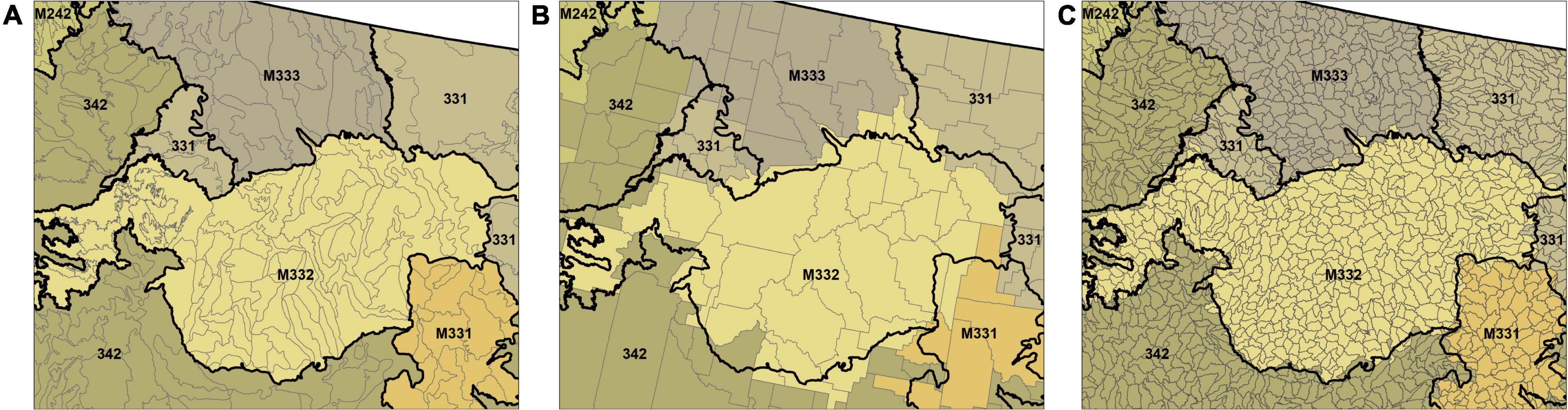
Figure 2. Illustration of provincial modeling domain and the (A) ecosubsections, (B) counties, and (C) watersheds they contain. Domains are assigned to modeling domain based on plurality of occupancy.

Response Data

The FIA updates and maintains a comprehensive database of forest inventory data across the U.S. based on a sample of plots, each representing approximately one acre of land. The database stores: tree-level measurements, including diameter and height; forest condition observations, including stand size and forest type; and a slew of calculated attributes, including basal area, volume, and biomass. The response data used in this analysis were extracted from the FIA database based on the most current measurement of each sampled plot at the time of download (2021 July 29). Only single intensity plots were used for this analysis to assure equal sampling probabilities across the populations. It should be noted that only the unit-level, model-based estimators require data from an equal probability sample design while all of the other estimators can account for unequal probability samples.

We used six different forest attributes as the focus for this analysis: forest area; live basal area (sqft) of trees 1.0 inch diameter and greater; number of live trees 1.0 inch diameter and greater; net board-foot (International 1/4-inch Rule) volume of live trees; cubic-foot volume of live trees; and biomass of live trees 1.0 inch diameter and greater, in tons (Burrill et al., 2021). All response data were expanded to the acre and adjusted for non-response at the plot-level; then summarized by the domain of interest. Thus, a plot that was partially sampled was assumed to be representative of the entire plot. A FIESTA function was used to extract and compile the data for each set of domains within each province. Plots were retrieved by intersecting states from a pre-built SQLite database and assigned to each province based on the Global Positioning System (GPS) plot location center.

Auxiliary Data

We used a limited set of auxiliary information for simplicity and consistency in the analyses. The data included two satellite-based classified images to represent current vegetative cover: (1) the 2016 USGS National Land Cover Dataset (NLCD), analytical tree canopy cover raster (Yang et al., 2018), including values from 1 to 100 representing the percent of tree canopy cover on the ground (tcc), and (2) the LANDFIRE 2014 Existing Vegetation Type (EVT) product (Rollins, 2009) re-classed to two classes, representing the dominant lifeform (1: tree; 2: non-tree) (tnt2). The NLCD layer was resampled to 90 m using the average of the original 30 m pixels to correspond to the acre-size FIA plot more closely (Nelson et al., 2009). Similarly, the LANDFIRE classified map was resampled to 90 m using the majority value within a focal window of 3 × 3 pixels.

The next three spatial layers are from the PRISM (Parameter-elevation Regressions on Independent Slopes Model) dataset (PRISM Climate Group, 2004), and represent influential climate patterns. The data layers include 30-year normals (Daly, 2002) describing average annual precipitation (ppt), average annual temperature (tmean), and average minimum temperature (tmin01) for the month of January over the period 1981–2010.

The last layer was chosen to understand the local altitude characteristics of the site, the LANDFIRE 2010, elevation dataset, derived from the National Elevation Dataset (NED), representing land height, in meters, above mean sea level (elev). This layer was resampled from 30 m resolution to 90 m using cubic-convolution interpolation.

A FIESTA function was used to assign values from each auxiliary spatial layer at each FIA plot location as well as calculate zonal mean statistics by domain within each province. The function uses the Geospatial Data Abstraction Library (GDAL) for low-level access to raster and vector geospatial data formats (GDAL/OGR contributors, 2019) and C++ to increase performance for large datasets. Predictors were standardized by subtracting the mean and dividing by the standard deviation for all observations within the modeling extent (i.e., province for small area estimates and domains for post-stratified and model-assisted estimates).

Estimators

Using the same input datasets, we generated estimates for three national datasets, using one estimator programmed in FIESTA and seven other estimators available from packages in the Comprehensive R Archival Network (CRAN²), integrated through FIESTA. This example illustrates FIESTA’s versatility to call upon a variety of estimation packages and also allows a user to compare output from multiple estimation strategies within a dashboard environment.

Mimicking FIA’s current estimation strategy, we produced post-stratified estimates based on the tnt2 variable through FIESTA’s Green-Book module which implements estimators documented in Bechtold and Patterson (2015). We also generated estimates based on a generalized regression estimator (GREG; Sarndal, 1984; McConville et al., 2020) that was implemented through FIESTA’s Model-Assisted module that makes use of the mase R package (McConville et al., 2018).

Through FIESTA’s Small-Area module, we integrated multiple estimators from the JoSAE R package (Breidenbach, 2018), including: area-level and unit-level empirical best linear unbiased prediction (EBLUP) estimators based on the Battese–Harter–Fuller unit-level model (Battese et al., 1988) and the Fay–Herriot area-level model (Fay and Herriot, 1979); a modified generalized regression (Rao and Molina, 2015); and a Horvitz–Thompson estimator (HT; Horvitz and Thompson, 1952). Area-level EBLUPs were also fit using the sae R package (Molina and Marhuenda, 2015). Note that unit-level estimators rely on models that relate specific plot-level responses to specific plot-level predictors, while area-level estimators rely on models that relate averaged area-level responses to averaged area-level predictors. To obtain the EBLUP estimates, the model parameters were estimated using restricted maximum likelihood within both the JoSAE and sae packages. We also generated hierarchical Bayesian (HB) estimates using the hbsae R package (Boonstra, 2012). We again used the Battese–Harter–Fuller model for the unit-level HB and the Fay–Herriot model for the area-level HB now with flat priors on all of the model parameters except the ratio of the between and within area variance where a half-Cauchy prior was used (White et al., 2021). The estimators described above are consolidated in Table 1, along with associated acronyms used for those estimators, as well as the publically available packages and functions called by FIESTA to construct those estimates. The source code for the back-end estimation done in FIESTA is publicly available via the FIESTAutils R package (Frescino et al., 2022), particularly in the SAest.pbar and MAest.pbar functions. In this implementation of FIESTA, we did not use any spatial covariance structure in our models, instead borrowing strength from ecologically similar areas serving as surrogates both for spatial proximity as well as similarity in other dimensions.

TABLE 1

Table 1. Estimators and associated short names/acronyms, R packages, and specific R functions within those packages.

Relevant predictors were selected for each small area model (both unit- and area- level, as well as the modified GREG) using the elastic net component of the gregElasticNet function in the mase R package (McConville et al., 2018). The elastic net is a regularized regression method, which controls for multicollinearity and performs variable selection (Zou and Hastie, 2005). The regularization is a linear combination of a lasso (L1) penalty and a ridge (L2) penalty. The mixing of these two penalties is controlled by alpha, where α = 1 is purely lasso and α = 0 is ridge. The variables were selected using α = 0.5. If no variables were selected, then the function was rerun with α = 0.2. If again, no variables were selected, NA was returned for all domains in the province. Variable selection was also implemented within mase for the GREGs, also using the elastic net procedure.

In addition, for area-level small area models, domains were identified up front where models would fail (e.g., where number of observations per domain were less than or equal to 1, or where variance of the response within that domain was 0) and returned with NA values.

Dashboards

We created three dashboards for this article, each associated with each different national dataset used in this article: an ecosubsection dashboard, a fifth-level, HUC10 watershed dashboard, and a county dashboard. The dashboards were built using the R packages flexdashboard (Iannone et al., 2020) and shiny (Chang et al., 2021). The dashboards utilize interactive spatial data mapping R packages such as leaflet (Cheng et al., 2021) in order to display results across the nation. The use of leaflet allows for users to zoom into regions of interest and click on interactive polygons to obtain estimate information at the domain level through the visual aid of an interactive map. We also use R packages such as ggplot2 (Wickham, 2016) and plotly (Sievert, 2020) to visualize estimates graphically and the R package DT (Xie et al., 2021) to create interactive data tables.

Results

Continental United States Processing

Estimates and standard errors from eight different estimators were generated across the conterminous US for six forest responses using the FIESTA R package. We ran a compiled set of FIESTA functions for each national dataset that performed: database extractions, auxiliary data summaries, and estimation preprocessing calculations, for integration with five different estimation R packages.

Estimates for all domains within all three national datasets were completed overnight using a Windows 10, 32.0 GB RAM, 64-bit, single core, i5-6300U CPU, 2.40 GHz processor. There was an average of 963 million, 90 m pixels across our three national datasets. Table 2 shows total times for one run by each national dataset, broken down by data compilation and estimation processes. Data compilation was a combination of plot data extraction and auxiliary spatial summaries, including pixel counts and zonal statistics for each domain across all provinces. Estimation processing included generation of small area estimates (and modified GREG) from JoSAE, sae, and hbsae packages, along with post-stratification from FIESTA, and GREG estimates from the mase package. Processing times also included a model selection routine from mase for all small area estimates (and modified GREG) and GREG estimates. On average, the GREG estimates consumed over 50% of the total estimation time. This was because a model was fit for each response for each domain (i.e., ecosubsection, county, watershed) within a province, different than small area estimates (and modified GREG), where only one model was fit for each response for each province. Processing times are further explored in Figure 3 by national dataset as a function of number of pixels for data compilation (with the number of pixels increasing as predictors are added), and as a function of number of domains for the estimation processes. In both cases, processing time follows a linear trend, although the slope of the trend varies by national dataset. The number of domains shows a slightly stronger influence on time.

TABLE 2

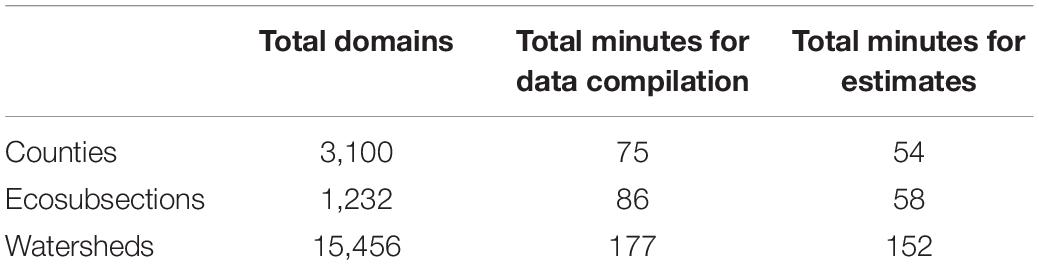
Table 2. Processing times for generating eight different estimates for five response variables across the three national datasets.

FIGURE 3

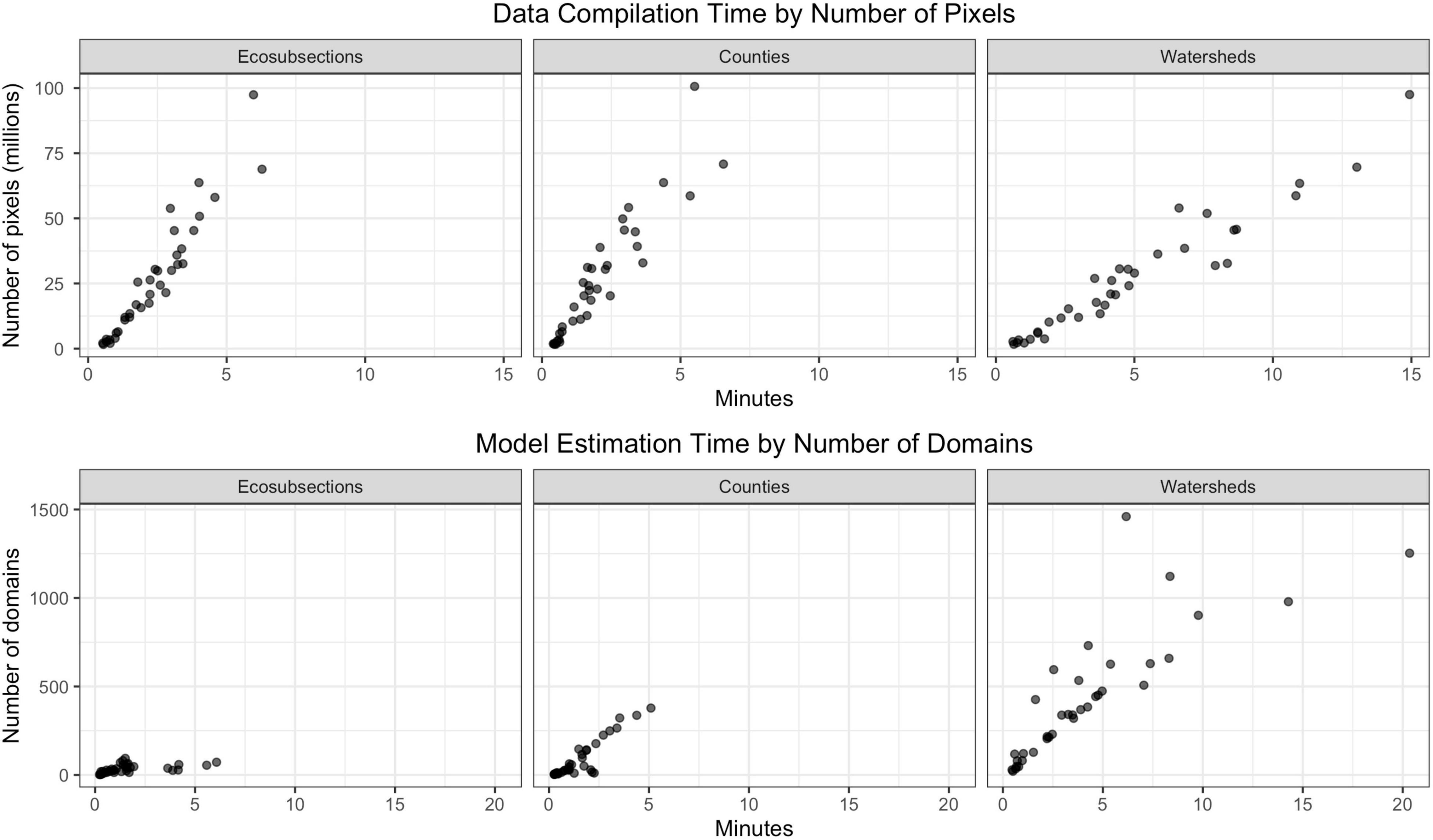
Figure 3. Nationwide processing times for data summarization and model estimation. Times are expressed in minutes by number of domains and number of pixels for each of the national datasets: ecosubsections, counties, and watersheds.

The estimation challenges posed by these three national datasets are explained by looking at a summary of the number of domains and plots within each province available to our suite of estimators. In general, ecosubsections are relatively large domains for which FIA would customarily rely on direct estimators. Contrarily, HUC 10 watersheds pose applications better suited for SAE. The sizes of counties in the US vary dramatically and are typically much smaller in the eastern US than they are in the western US. The distribution of number of domains in each province (Figure 4A) shows that on average, area-level models had over 30 domains to work with for the county and ecosubsection national datasets, whereas the smaller watershed delineation resulted in an average of over 200 domains per area-level model. However, both the ecosubsection and county national datasets posed challenges for the area-level models in instances where number of domains fell into the single digits. Area-level models occasionally failed in production runs, most often for domains for which there was a combination of too few domains and too weak a relationship with auxiliary data at the area-level. For the unit-level models (both model-assisted and small area) the median number of plots available (Figure 4B) was over 100, well within the recommended sample sizes for direct estimators. However, for watersheds, the average number of plots across provinces was only around 3. Figure 4C reflects how many provinces had extremely small numbers of plots at the domain level. For ecosubsections, very few did, with the minimum never falling below about 10 plots. However both the county and watershed national datasets had a number of provinces where only 1 plot was available in some of the domains, precluding the use of area-level models in those cases. Finally, the maximum number of plots by domain within province in Figure 4D illustrates how rarely there are a sufficient number of plots within watersheds for direct estimation.

FIGURE 4

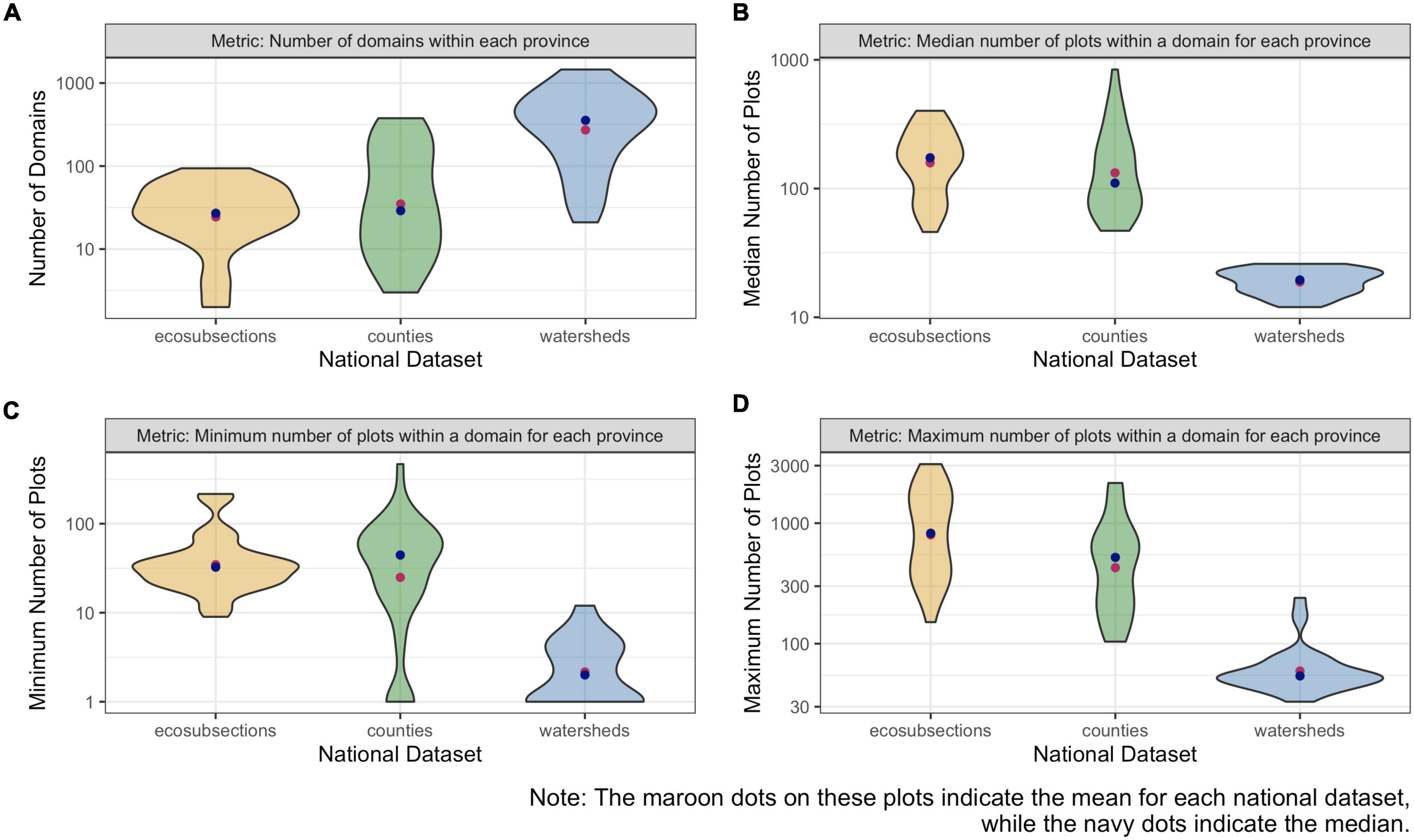
Figure 4. Violin plots reflecting the distribution, by national dataset, of (A) number of domains within the provinces, as well as (B) median, (C) minimum, and (D) maximum number of plots per domain within the provinces. The maroon dots on these plots indicate the mean for each national dataset, while the navy dots indicate the median. The color of the violin plot indicates the national dataset it represents: yellow for ecosubsections, green for counties, and blue for watersheds. Note that the y-axis is spaced on a log10 scale.

Variable selection was part of the nationwide processing to minimize model failure rates and improve model specification. Although all the auxiliary data made available to the estimation modules were known to have some relationship to FIA response variables, that relationship is naturally different across provinces and estimators. To provide a sense of variable importance nationally, Figure 5 illustrates the percentage of times each predictor variable was selected by the elastic net for unit-level and area-level EBLUPs of basal area for the watershed national data set. The tcc and tnt2 predictors are most often included in both unit- and area-level models, with ppt, elev, tmean, and tmin01 selected less often. With the weaker relationships at the unit-level than the area-level, the elastic net most commonly selected 2 predictors at the unit-level and 4 predictors at the area-level. Strongly correlated predictors, such as tcc and tnt2, exhibited a grouping effect where they were either all included or excluded from the model, a known phenomenon for the elastic-net procedure (Zou and Hastie, 2005).

FIGURE 5

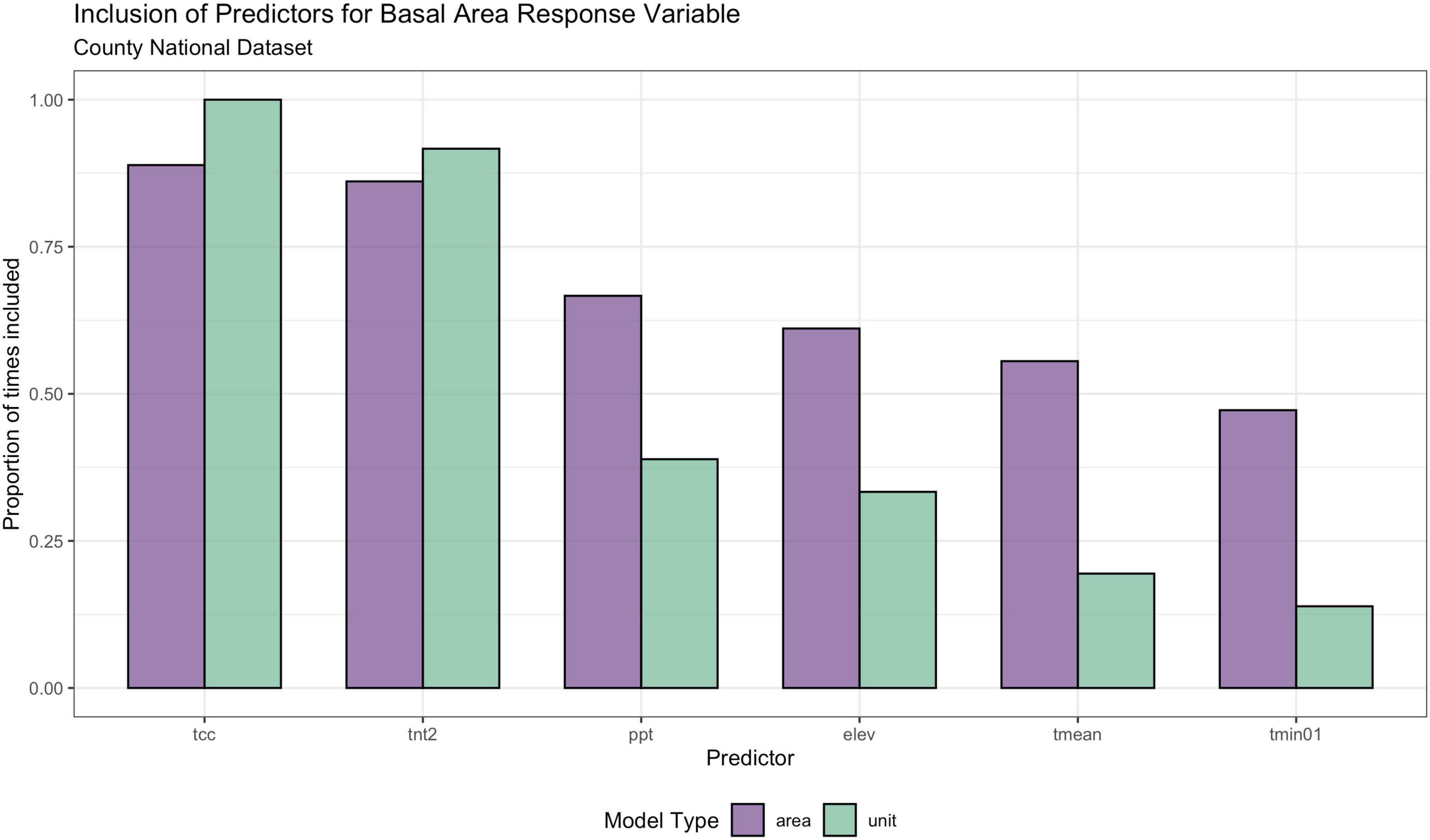
Figure 5. Proportion of times each of the predictor variables was selected for area-level (purple) and unit-level (green) model-based estimators (both EBLUP and HB) applied to the county national dataset through the elastic net variable selection process used in this paper.

Results from this nationwide processing are represented by Figures 6A–C, which depict the small area estimates of basal area for ecosubsections, counties, and watersheds, respectively. The estimator used is the sae area-level EBLUP. Missing values were filled with JoSAE’s area-level EBLUP and then with the Horvitz-Thompson estimator if needed. This process filled all holes except for 12 ecosubsections. For those 12 ecosubsections, there were no sampled plots with response variable greater than zero, so these were given a value of zero.

FIGURE 6

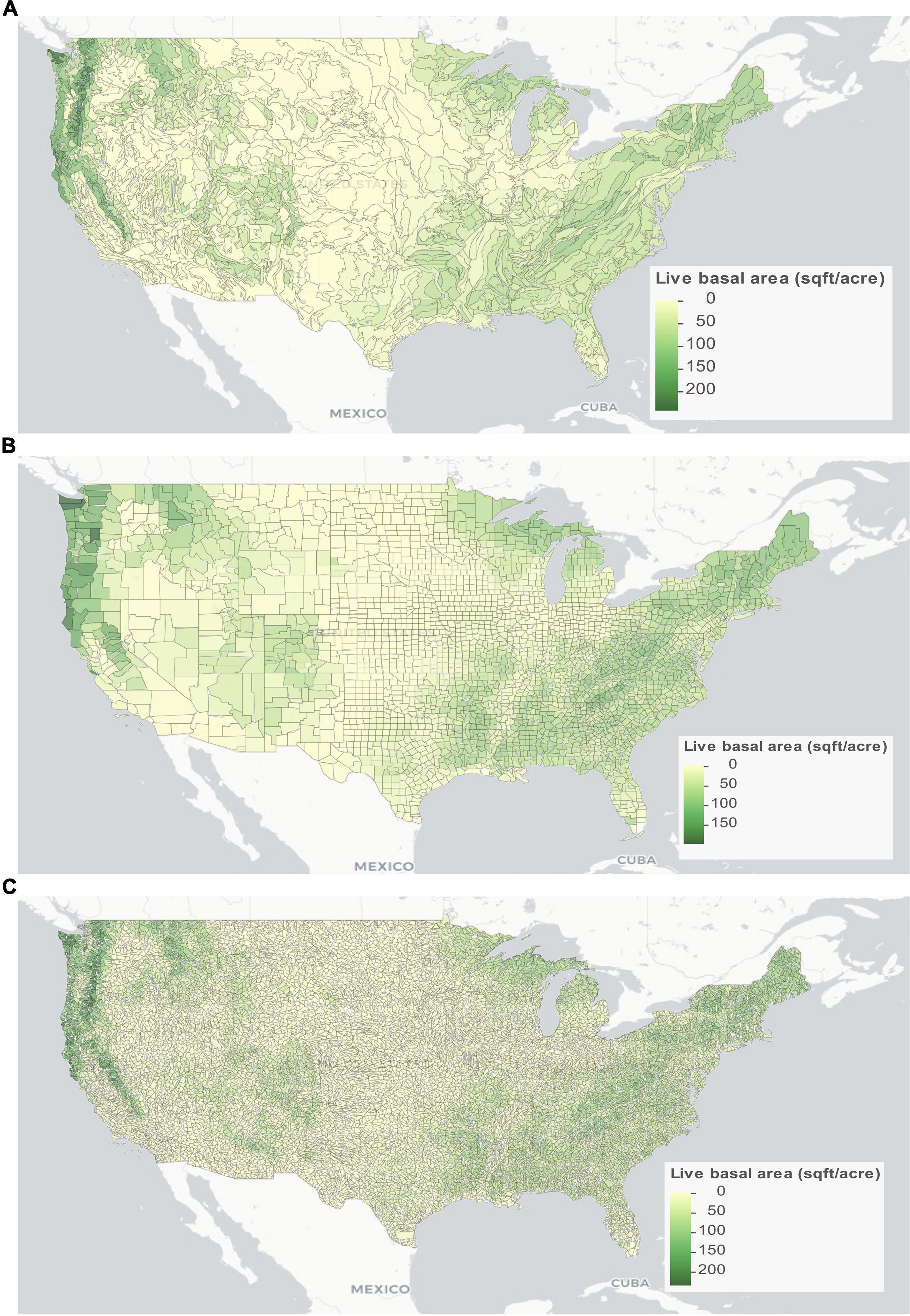
Figure 6. Small area estimates of basal area for (A) ecosubsections, (B) counties, and (C) watersheds based predominantly on area-level EBLUPs.

Precision and Bias

With FIESTA’s ability to compute a wide range of estimators, we can now easily make comparisons of the performance of different estimation approaches. Figure 7 displays the median relative efficiency of each of the eight estimators of basal area over all domains across continental United States (CONUS). Numbers in each cell reflect the median ratio of the variance of the estimates derived under the estimator named in the column over the variance of the estimator named in the row. Reading an estimator’s median variance ratio down the column allows one to see its median variance ratio where it is in the numerator, while reading an estimator’s median variance ratio across the row allows one to see the ratio where it is in the denominator. Red cells indicate higher valued ratios, meaning that the estimator in the denominator is less variable, while blue cells indicate lower valued ratios, meaning that the estimator in the numerator is less variable.

FIGURE 7

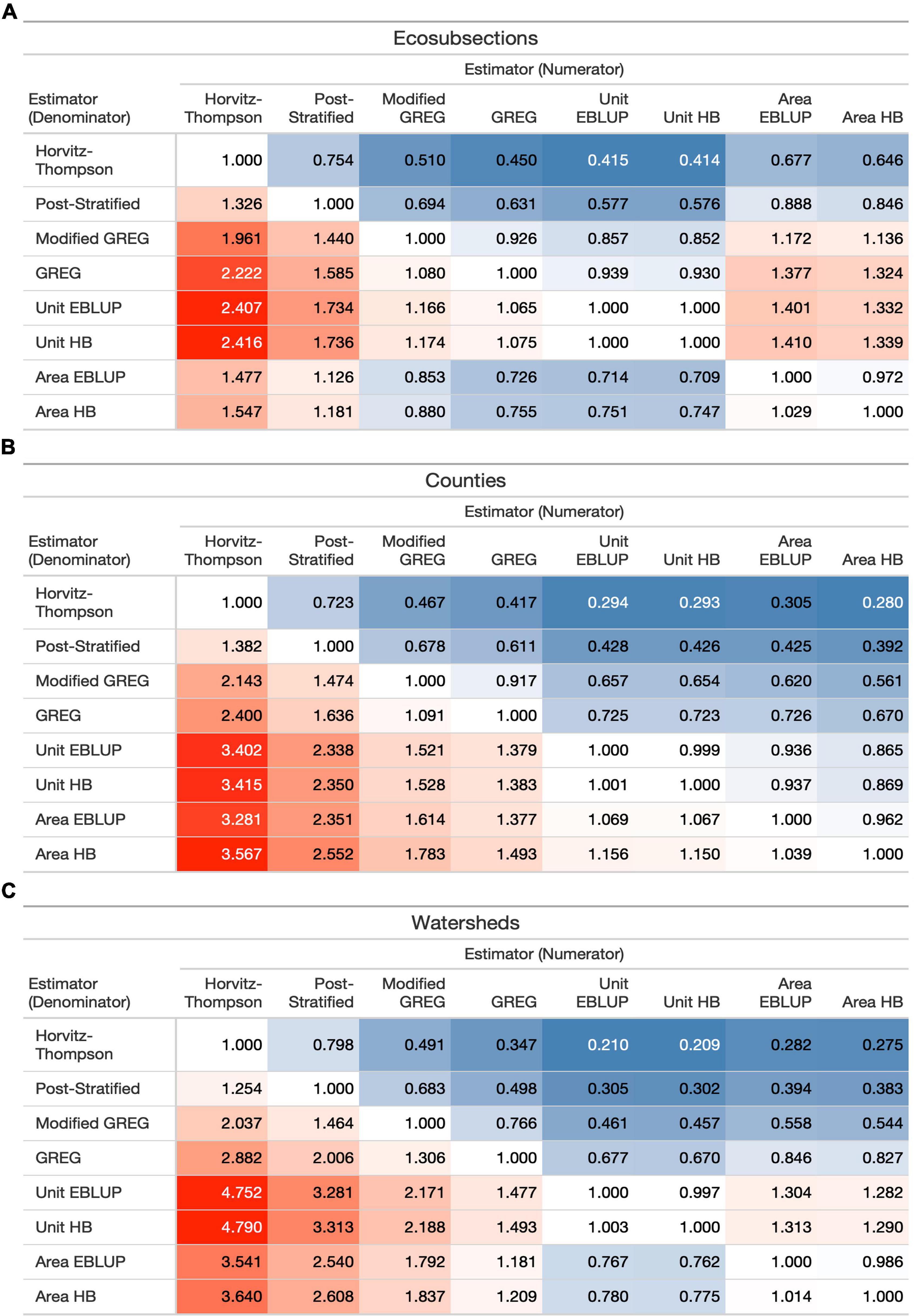
Figure 7. The relative efficiency of each of the eight estimators for basal area averaged over (A) ecosubsections, (B) counties, and (C) watersheds for the entire study region. Numbers in each cell reflect the variance of the estimates derived under the estimator named in the column divided by the variance of the estimator named in the row. Shades of blue reflect values less than 1, with the deepest blue set at the minimum value for that specific table. Conversely, shades of red reflect values greater than 1 with the deepest red set at the maximum value for that specific table.

From Figure 7, we see that the direct estimators tend to have higher median variance estimates than the indirect estimators. Among the direct estimators, the modified GREG and the GREG, which incorporate more of the auxiliary data, tends to be less variable than the HT, which utilizes no auxiliary data, and the PS, which uses one categorical, auxiliary data layer. The variance estimates tend to be slightly lower when modeling at the domain (GREG) instead of the province (modified GREG), which may be explained by the GREG’s tendency to underestimate the variance when using an internal model (Kangas et al., 2016). In general, the best direct estimator was the GREG and its average relative efficiency over a Horvitz Thompson estimator for the three national datasets ranged from 0.35 to 0.45. In fact, the GREG is fairly competitive with the indirect estimators and in some cases results in a smaller median variance estimate, especially for ecosubsection domains which tend to have larger sample sizes. Among the indirect estimators, the HB and EBLUP approaches show strong agreement, which isn’t surprising given the moderately sized samples, large number of domains, and weakly informative prior on the ratio of the within and between variation. Relative efficiencies range from 0.96 to 1.0.

The relative gain in precision we obtain using any one of these estimators is further clarified as a function of sample size in Figures 8A–C for ecosubsections, watersheds, and counties respectively. Here, smoothed curves of standard errors for basal area are plotted against sample size for each estimator. We see a consistent pattern across national datasets. As expected the direct estimators yield the highest variances with direct being the worst, followed by improvements with post-stratification, modified GREG, and GREG. Also as expected, the model-based estimators show considerable improvement over smaller sample sizes, with the unit-level EBLUP and HB, as well as the area-level EBLUPs and HB yielding similar results with a slight improvement from the unit-level estimators. Similar patterns were seen for the other response variables.

FIGURE 8

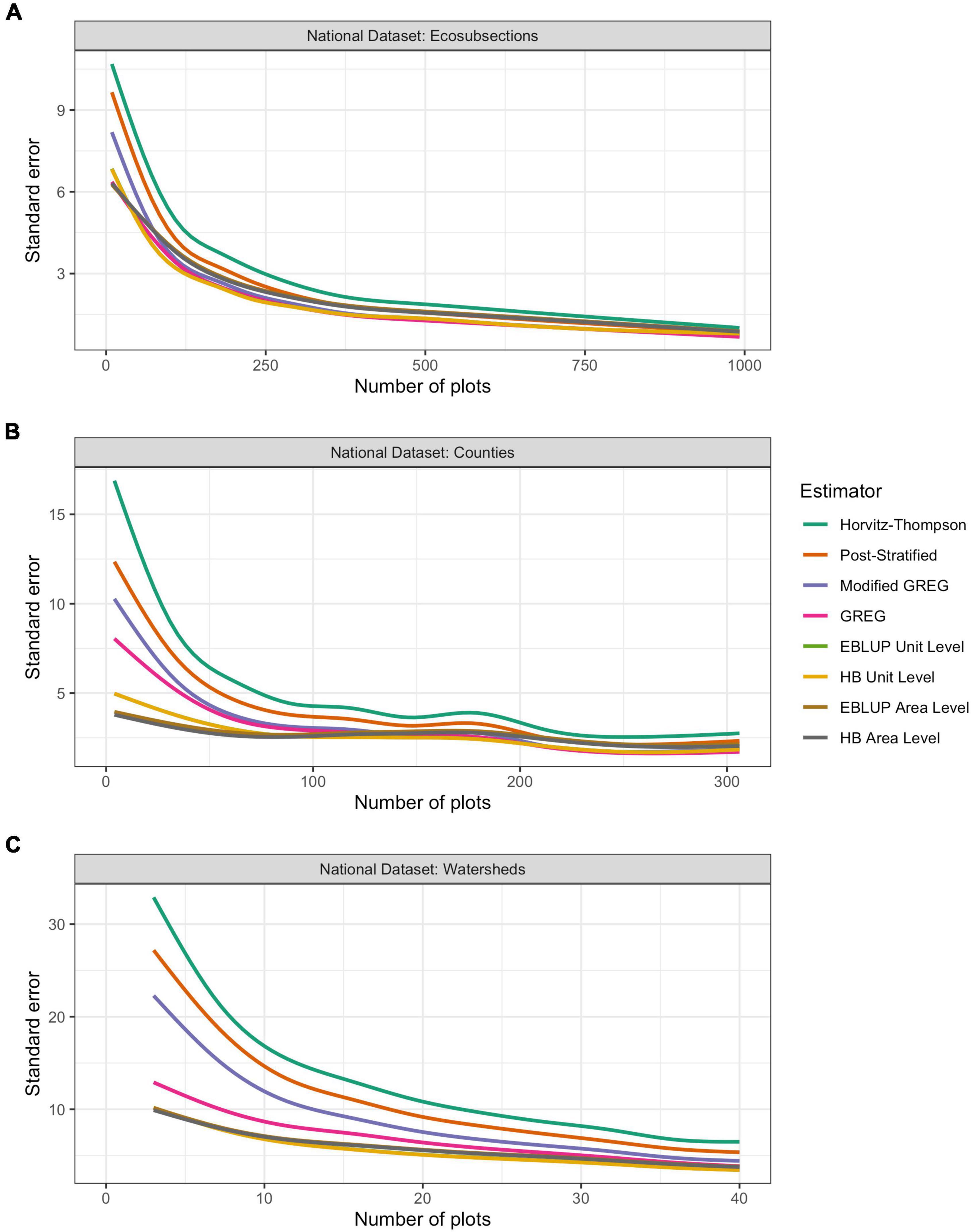
Figure 8. Smoothed standard errors by number of plots for all estimates of basal area obtained over (A) ecosubsections, (B) counties, and (C) watersheds. The lines used to represent the data were created with a generalized additive model using smoothing splines with a cubic spline basis. The y-axis represents the standard error of each estimator and the x-axis represents the number of plots within the domain of interest. For each plot, we trimmed the number of plots to the 0.95 quantile in order to avoid high leverage points in the smoothing algorithm. This 0.95 quantile point was found to be 991 for ecosubsections, 277 for counties, and 40 for watersheds. These plots were created only for regions where no estimators produced NA values.

Overall, between the indirect, area-level and indirect, unit-level estimators, neither is consistently more efficient than the other. However, Figure 9 illustrates the potential for model misspecification in unit-level models. Figure 9A we see the challenging relationship between basal area and tcc at the unit level for province M221 with counties as the national dataset. Figure 9B depicts the clear linear relationship between the same variables, in the same province and with the same national dataset, but at the area level. The consequences of using the unit- versus the area-level estimators are also depicted where the Horvitz Thompson estimates are plotted against the unit-level EBLUP in Figure 9C, and against the area-level EBLUP in Figure 9D. The potential for over predicting biomass in the unit level instance is apparent at the zero tick for the x-axis. Nationally, this pattern persists for all the unit-level models (EBLUP, HB, and modified GREG) as shown in Figure 10. Negative estimates are also occasionally provided by the unit-level models.

FIGURE 9

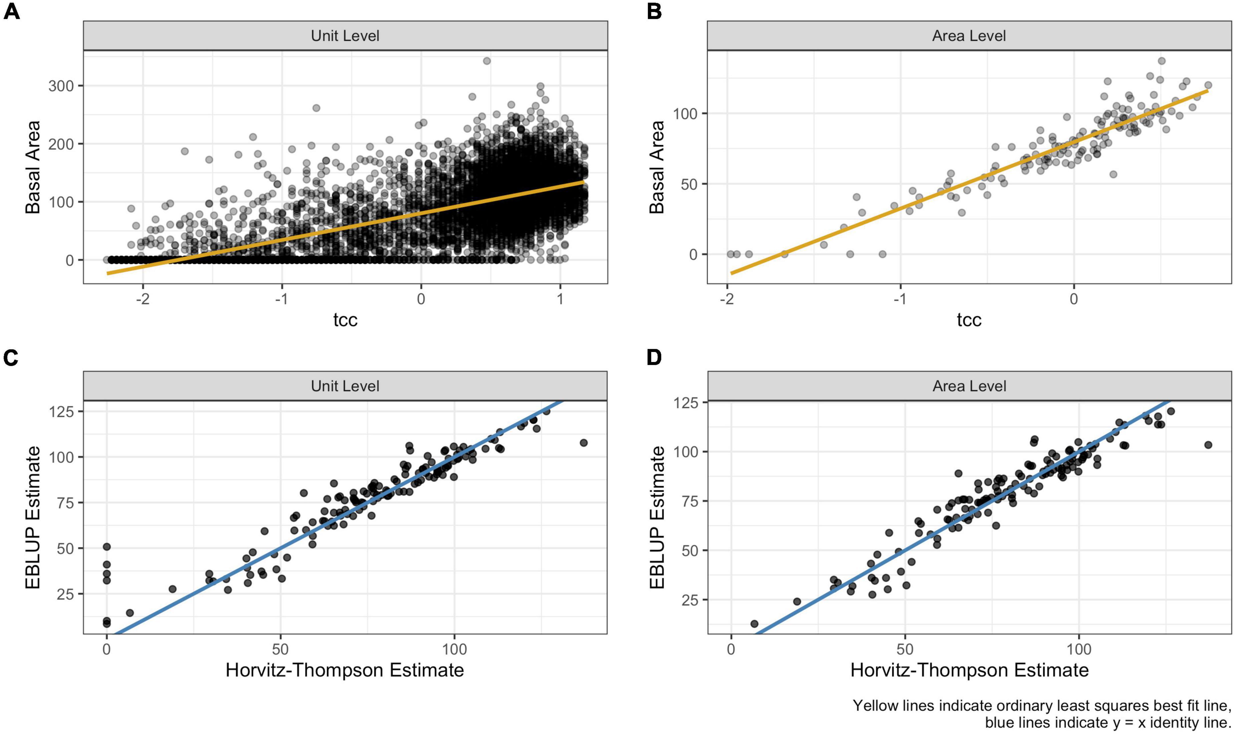
Figure 9. The relationship between a response variable (basal area) and a predictor variable (total canopy cover, “tcc”). (A) Depicts the relationship between basal area and tcc at the unit level for province M221 with counties as the national dataset. (B) Depicts the relationship between the same variables, in the same province and with the same national dataset, but at the area level. (C) Unit and (D) area-level EBLUP estimates compared to the Horvitz–Thompson estimates in province M221 for the county domains. On plots (A,B), the yellow line indicates the ordinary least squares best fit line and on plots (C,D) the blue line is the identity line.

FIGURE 10

Figure 10. Estimates of basal area (sqft) from each estimator compared to the Horvitz–Thompson for all counties in across the conterminous US.

Dashboards

While we are able to draw several useful conclusions using the static tables and figures provided in the results above, the FIESTA dashboards provide an interactive venue for users to explore these estimators in greater depth. For ecosubsections, counties, and watersheds, these can be found at https://ncasi-shiny-tools.shinyapps.io/Ecosubsections/, https://ncasi-shiny-tools.shinyapps.io/Counties/, and https://ncasi-shiny-tools.shinyapps.io/Watersheds/, respectively. In these dashboards, the tables and figures adapt dynamically to the user’s choices for state, attributes, and estimators.

Figure 11 gives an example of the watershed dashboard. From the “Maps and Data” tab (A) the user can select the state, the forest attribute, and which of the design- or model-based estimates they are interested in. Clicking on any individual watershed reveals the watershed name, as well as the estimate and standard error for the attribute selected. Then from the “Estimator Comparisons” tab, the user can compare the performance of any of the estimators for their attribute and state of choice through graphs depicting the distribution of estimates and standard errors, as well as a table of relative efficiencies comparable to Figure 7C, but for the users specified state and attribute.

FIGURE 11

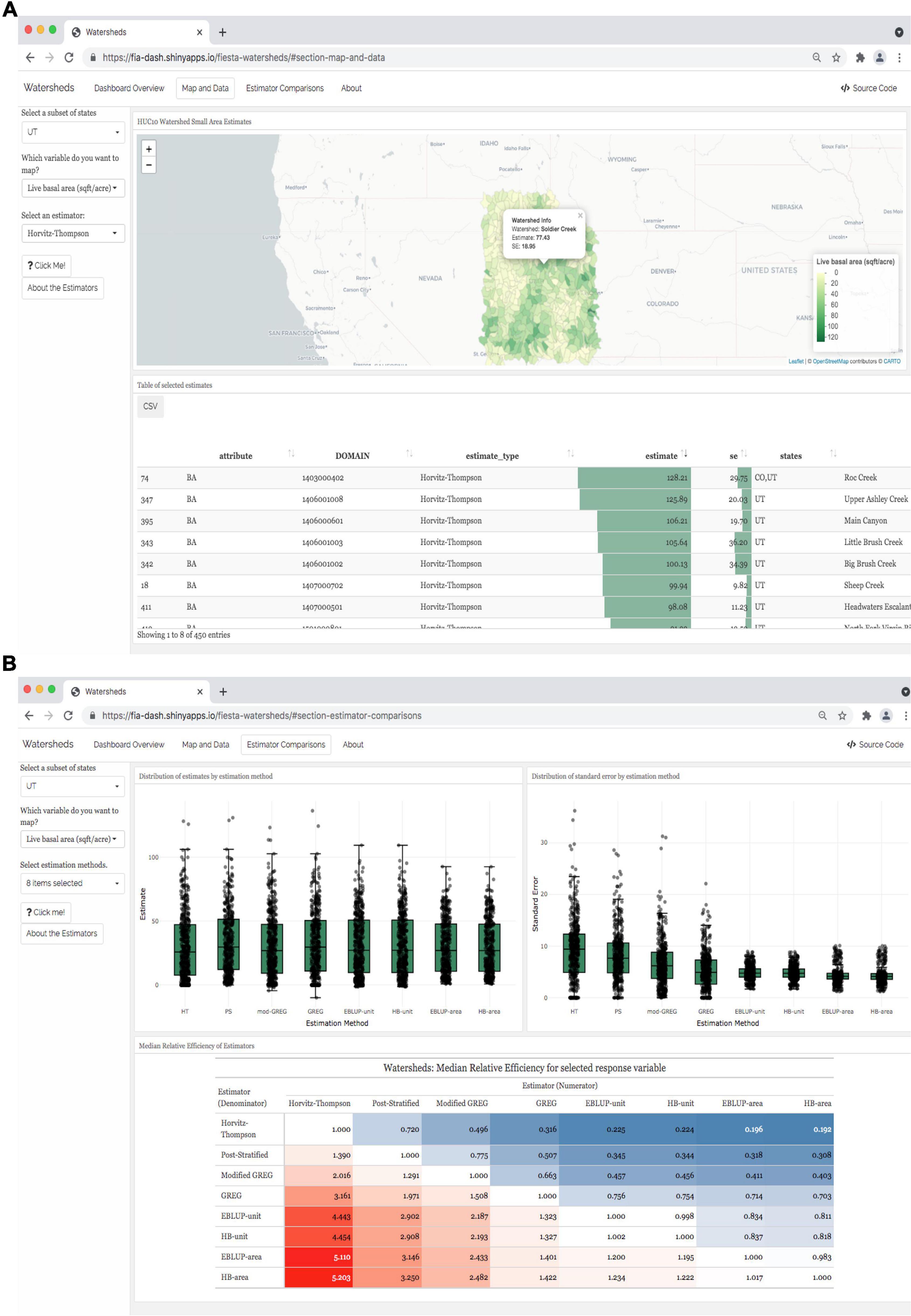
Figure 11. Example views from the watershed dashboard available at https://ncasi-shiny-tools.shinyapps.io/Watersheds/. From the Maps and Data Tab (A) the user can select a state, which variable they are interested in and specify which of the design- or model-based estimates they would like to see. Then from the Estimator Comparisons Tab (B), the user can compare the performance of any of the estimators for their variable and state of choice through graphs depicting the distribution of estimates and standard errors, as well as a table of relative efficiencies comparable to Table 2, but for the users specified state and attribute. Dashboards in the same format have also been constructed for ecosubsections and counties, which can be accessed at https://ncasi-shiny-tools.shinyapps.io/Ecosubsections/, and https://ncasi-shiny-tools.shinyapps.io/Counties/ respectively.

Discussion

In this paper, we demonstrated a process for using FIA’s extensive, strategic-level, national database for generating estimates within non-traditional extents across the US, and present results from a wide range of alternative estimators in a user-friendly dashboard environment. The study of SAE and other alternative estimation strategies for forest inventories is rapidly evolving. FIESTA offers the flexibility to accommodate these estimation strategies, along with integrating unique responses, multiple auxiliary data sources, and different model fitting specifications, to continue this evolution through user-friendly delivery systems, and it reveals a pathway for using FIA data in more creative ways for answering forest research questions. The demonstration presented in this paper of a nationwide processing system, precision analyses, and dashboards, answered several questions surrounding SAE for forest inventories, but also posed additional topics warranting further research.

Inventory Attributes

Here we constructed estimates of six key FIA attributes to demonstrate the process. But FIA has information on hundreds of attributes and FIESTA can access any of these from FIA’s extensive database to construct estimates of interest. FIA’s current estimation process does not just focus on one variable at a time to conduct specific inference, rather it reports on a multitude of estimates that must be internally consistent, accommodating generic inference. FIESTA can mimic this process using post-stratification through its Green-Book or Model-Assisted modules, and thus be compatible with current estimates. However, the opportunity exists to improve precision in these direct estimates by simply moving to other model-assisted methods such as a GREG where additional auxiliary data in either continuous or discrete format can be used, and still retain the ability for generic inference that is important to any sample survey organization. Going beyond that, though, there are instances where specific inference is called for and small area estimates are constructed through model-based methods targeting a single attribute. FIESTA has the ability to accommodate these types of problems through its SA module. More work is needed to provide guidelines on transitioning from model-assisted to model-based estimators in cases of specific inference. In addition, more work is needed in small domains to model FIA variables jointly to preserve their ecological consistency.

Auxiliary Data

The development and distribution of alternative auxiliary data layers relevant to forest inventory is an active area of research. The set of predictors used here provide a sensible place to start for estimates of forest status. But finer resolution and higher quality data is coming online rapidly and could offer substantial improvements in precision of inventory estimates. (See Lister et al., 2020 for a review of evolving remotely sensed products.) In addition, looking beyond status to variables that reflect change, such as growth removals and mortality, requires a very different set of auxiliary data in order to establish good models between the response and predictors (e.g., Coulston et al., 2021). FIESTA is designed to use any appropriately scaled auxiliary data and allows the user to easily assess the contribution of a given set of predictors on the precision of an estimator. Although critical to defining the sample design, a nationwide layer depicting sampling intensity by year has yet to be developed and is needed to enable the use of all inventory plots, not just those collected at standard spatial and temporal scales.

Estimators

The eight estimators applied to the three national datasets illustrate the ability of FIESTA to draw from numerous alternative estimation packages in R. In this case, the packages mase, JoSAE, sae, and hbsae were called upon. There are many options associated with these packages that can be tapped, while FIESTA was also designed to plug-and-play alternative packages and arguments as needed. As new estimation packages, or user-built analysis functions become available, they can be added to the comparison to continue to get the best results for the questions asked.

This nationwide processing of domains of different sizes over CONUS revealed some important information about the efficiency of different estimators given the set of auxiliary data provided. Evaluated at a national scale the increasingly superior precision performance of post-stratification, modified GREG, and GREG is not surprising. However, the smaller variances produced by GREG over the modified GREG warrant further investigation. Also, the precision gains from model-based estimators over the design-based estimators for very small sample sizes is also not surprising. And although unit-level models produced estimates compatible with direct estimates in areas where direct estimates were reliable, the effect of model mis-specification on bias in estimates should be more fully explored. Important to note are the gains that can be realized from model-assisted methods such as GREG for smaller sample sizes while still maintaining asymptotic unbiasedness even if the models are mis-specified, and retaining the ability to conduct generic inference. This automated processing also makes tests for simply improving FIA’s current post-stratification process with new auxiliary data much easier.

Model Fitting

While it is ideal to construct individual models for every variable over every geographic region, a production system needs to be automated and robust to model mis-specification. For example, while it is good to have a number of auxiliary data layers available for estimation models, variable selection techniques, like the elastic net employed here, can help ensure only meaningful data are contributing to the estimation process. This paper demonstrates the strides that have been taken to automate model-fitting strategies such as variable selection and handle inevitable issues that arise from non-convergence, insufficient data, and small numbers of domains in a production environment. However, more work should be done to evaluate variable contributions, especially in the presence of collinearity and complex, non-linear relationships.

In these nationwide runs, borrowing strength occurred at the ecological province level. However, FIESTA is set up to allow a user to specify a different borrowing strategy. For example, White et al. (2021) suggest, for some response variables, ecological sections may provide a better borrowing strategy for small area models, as they are smaller, more homogenous regions. Alternatively, management strategies across different forest land ownerships might suggest a reason to distinguish borrowing across public vs. private land ownerships. In addition, users may have access to higher quality or higher resolution auxiliary data in their specific geographic region and wish to constrain the borrowing area to the extent of the better data. In addition, as future work we hope to add more flexible small area models to FIESTA in order to account for spatial structure, as these models have been shown to increase precision in a forestry context (Ver Planck et al., 2018).

Computing and Delivery

The dashboards presented here provide a mechanism for scientists, statisticians, and other users to explore potential for precision gains and for setting expectations in geographically specific regions of the country. All the graphics presented in the results at the national scale can be subset for specific provinces or states within the dashboards. The dashboards also demonstrate an opportunity through which users of forest inventory data can explore small area perimeters and specific forest inventory variables for which estimates are needed until such time as interactive online tools are available for them to fulfill their information needs. Following the same process shown here, estimates will soon be derived for past and present wildfire perimeters across the nation to obtain a sample-based picture of resources lost to fire. Although similar strategies will be used, new challenges arise from the diversity of sizes and extents across non-contiguous boundaries.

All estimates, tables, graphics, maps, and dashboards were processed within the R environment. This project highlights the power, versatility, and magnitude of R. Although some aspects may be more efficient in other software, keeping it in one platform minimizes complexity in programming and analysis. Work is underway to increase FIESTA’s processing speed through conversion of spatial functions to Python. Beyond FIESTA access provided to novice users through dashboards like those illustrated here, plans for other distribution veins proceed as follows: for expert users, the FIESTA package is currently distributed on GitHub³, and will soon be available on CRAN (see footnote 2); for novice-to-intermediate users, a stand-alone desktop application of FIESTA is currently rolling out; and for Esri users, FIESTA is being integrated into ArcGIS Pro. In addition to the backend estimation code already available in the FIESTAutils R package on CRAN, all other code used in this paper will be available through the open-source delivery of FIESTA along with additional resources in vignettes and the associated FIESTAnalysis package which provides wrapper functions to streamline analyses using FIESTA functions and includes estimate diagnostics found in this paper.

Conclusion

Leveraging a decade’s worth of statistical and computational research on FIA’s flexible estimation engine, FIESTA, we demonstrated a process for translating information in FIA’s extensive national database to interactive dashboards through which users can easily access statistically defensible estimates anywhere in the conterminous US. We combined FIA plot data with national remotely sensed data layers to produce estimates over collections of small domains using published and widely accepted model-assisted and SAE methodologies. Based on national analyses, the order of estimator performance for smaller sample sizes (ranging from best to worst precision) was unit-level small area models, area-level small area models, generalized regression estimators, modified generalized regression estimators, post-stratification, and Horvitz–Thompson. But the gains in precision for unit-level over the area-level small area models do not offset the potential for bias due to model mis-specification in unit-level models. Further, for moderate sample sizes, substantive gains in precision can be realized by simply moving beyond post-stratification to alternative model-assisted estimators like generalized regression, to capitalize on information from auxiliary data and retain the advantages of direct design-based estimators. The extensive dataset of estimates available through the dashboards provides the opportunity for others to compare estimators and explore precision expectations over specific domains and geographic areas of the country. The dashboards also provide a forum for future development and analyses. This project also illustrates one pathway to moving statistical research into operational inventory processes, providing a vehicle through which FIA scientists and analysts can share their own tools and analytical processes with others.

Data Availability Statement

The datasets presented in this study can be found in online repositories. The names of the repository/repositories and accession number(s) can be found below: the datasets generated and analyzed for this study can be found in the publicly available dashboards created for this study. The dashboards for ecosubsections, counties, and watersheds can be found at: https://ncasi-shiny-tools.shinyapps.io/Ecosubsections/, https://ncasi-shiny-tools.shinyapps.io/Counties/, and https://ncasi-shiny-tools.shinyapps.io/Watersheds/, respectively.

Author Contributions

TF and GM: conceptualization, methodology, validation, and writing—original draft preparation. TF, GW, and JT: software. TF: formal analysis and data curation. TF, GM, and KM: investigation. GM and TF: resources. TF, GM, KM, and GW: writing—review and editing. GW: visualization. KM: supervision. GM: project administration and funding acquisition. All authors read and agreed to the published version of the manuscript.

Funding

KM’s contributions were supported by the USDA Forest Inventory and Analysis Program (via agreement 19-JV-11221638-112).

Conflict of Interest

GW is employed by RedCastle Resources, Inc.

The remaining authors declare that the research was conducted in the absence of any commercial or financial relationships that could be construed as a potential conflict of interest.

Publisher’s Note

All claims expressed in this article are solely those of the authors and do not necessarily represent those of their affiliated organizations, or those of the publisher, the editors and the reviewers. Any product that may be evaluated in this article, or claim that may be made by its manufacturer, is not guaranteed or endorsed by the publisher.

Acknowledgments

We want to thank Madelon Basil, Isabelle Caldwell, Alex Flowers, Sam Olson, and Olek Wojcik for creating the template used in the FIESTA dashboards.

Footnotes

1. ^ https://www.fia.fs.fed.us/tools-data/index.php
2. ^ https://cran.r-project.org/
3. ^ https://github.com/USDAForestService/FIESTA

References

Battese, G. E., Harter, R. M., and Fuller, W. A. (1988). An error component model for prediction of county crop areas using survey and satellite data. J. Am. Stat. Assoc. 83, 28–36. doi: 10.1080/01621459.1988.10478561

CrossRef Full Text | Google Scholar

Bechtold, W. A., and Patterson, P. L. (2015). The Enhanced Forest Inventory and Analysis Program National Sampling Design and Estimation Procedures. Asheville, NC: U.S. Department of Agriculture, Forest Service, Southern Research Station, doi: 10.2737/SRS-GTR-80

CrossRef Full Text | Google Scholar

Bell, D. M., Wilson, B. T., Werstak, C. E., Oswalt, C. M., and Perry, C. H. (2022). Examining k-nearest neighbor small area estimation across scales using national forest inventory data. Front. For. Glob. Change 5:763422. doi: 10.3389/ffgc.2022.763422

CrossRef Full Text | Google Scholar

Boonstra, H. J. (2012). hbsae: Hierarchical Bayesian Small Area Estimation. R package version 1.0. Available Online at: https://CRAN.R-project.org/package=hbsae (accessed July 1, 2021).

Google Scholar

Breidenbach, J. (2018). JoSAE: Unit-Level and Area-Level Small Area Estimation. R package version 0.3.0. Available Online at: https://CRAN.R-project.org/package=JoSAE (accessed July 1, 2021).

Google Scholar

Burrill, E. A., DiTommaso, A. M., Turner, J. A., Pugh, S. A., Christensen, G., Perry, C. J., et al. (2021). FIA Database Description and User Guide for Phase 2 (version: 9.0.1). [WWW Document]. St Paul MN: U.S. Department of Agriculture, Forest Service, North Central Research Station.

Google Scholar

Cao, Q., Dettmann, G. T., Radtke, P. J., Coulston, J. W., Derwin, J. M., Thomas, V. A., et al. (2022). Increased precision in county-level volume estimates in the U.S. National Forest Inventory with area-level SAE. Front. For. Glob. Change 5:769917. doi: 10.3389/ffgc.2022.769917

CrossRef Full Text | Google Scholar

Chang, W., Cheng, J., Allaire, J., Sievert, C., Schloerke, B., Xie, Y., et al. (2021). shiny: Web Application Framework for R. R package version 1.6.0. Available Online at: https://CRAN.R-project.org/package=shiny (accessed July 1, 2021).

Google Scholar

Cheng, J., Karambelkar, B., and Xie, Y. (2021). leaflet: Create Interactive Web Maps with the JavaScript ‘Leaflet’ Library. R package version 2.0.4.1. Available Online at: https://CRAN.R-project.org/package=leaflet (accessed July 1, 2021).

Google Scholar

Cleland, D. T., Freeouf, J. A., Keys, J. E. Jr., Nowacki, G. J., Carpenter, C., and McNab, W. H. (2007). Ecological Subregions: Sections and Subsections of the Conterminous United States [1:3,500,000] [CD-ROM]. Sloan, A.M., cartog. Gen. Tech. Report WO-76. Washington, DC: U.S. Department of Agriculture, Forest Service.

Google Scholar

Coulston, J. W., Green, P. C., Radtke, P. J., Prisley, S. P., Brooks, E. B., Thomas, V. A., et al. (2021). Enhancing the precision of broad-scale forestland removals estimates with small area estimation techniques. For. Int. J. For. Res. 50, 1–15. doi: 10.1093/forestry/cpaa045

CrossRef Full Text | Google Scholar

Daly, C. (2002). Climate division normals derived from topographically-sensitive climate grids. 13th AMS Conf. on Applied Climatology. Portland, OR: American Meteorological Society.

Google Scholar

Dettmann, G. T., Radtke, P. J., Coulston, J. W., Green, P. C., Wilson, B. T., and Moisen, G. G. (2022). Review and synthesis of estimation strategies to meet small area needs in forest inventory. Front. For. Glob. Change 5:813569. doi: 10.3389/ffgc.2022.813569

CrossRef Full Text | Google Scholar

Fay, R. E., and Herriot, R. A. (1979). Estimates of income for small places: an application of James-Stein procedures to census data. J. Am. Stat. Assoc. 74, 269–277. doi: 10.2307/2286322

CrossRef Full Text | Google Scholar

Filippelli, S. K., Falkowski, M. J., Hudak, A. T., Fekety, P. A., Vogeler, J. C., Khalyani, A. H., et al. (2020). Monitoring pinyon-juniper cover and aboveground biomass across the Great Basin. Environ. Res. Lett. 15:025004. doi: 10.1088/1748-9326/ab6785

CrossRef Full Text | Google Scholar

Frescino, T. S., Moisen, G. G., Patterson, P. L., Toney, J. C., and Freeman, E. A. (2020). “Demonstrating a progressive FIA through FIESTA: A bridge between science and production,” in Celebrating progress, possibilities, and partnerships: Proceedings of the 2019 Forest Inventory and Analysis (FIA) Science Stakeholder Meeting; November 19–21, 2019; Knoxville, TN. e-Gen. Tech. Rep. SRS–256, ed. T. J. Brandeis (Asheville, NC: U.S. Department of Agriculture Forest Service, Southern Research Station), 199–200.

Google Scholar

Frescino, T. S., Toney, C., and White, G. W. (2022). FIESTAutils: Utility Functions for Forest Inventory Estimation and Analysis. R package version 1.0.0. Available Online at: https://CRAN.R-project.org/package=FIESTAutils (accessed April 5, 2022).

Google Scholar

Gaines, G. C., and Affleck, D. L. R. (2021). Small area estimation of postfire tree density using continuous forest inventory data. Front. For. Glob. Change 4:761509. doi: 10.3389/ffgc.2021.761509

CrossRef Full Text | Google Scholar

GDAL/OGR contributors (2019). GDAL/OGR Geospatial Data Abstraction software Library. Beaverton, Oregon: Open Source Geospatial Foundation.

Google Scholar

Gillespie, A. J. R. (1999). Rationale for a National Annual Forest Inventory Program. J. For. 97, 16–20. doi: 10.1093/jof/97.12.16

CrossRef Full Text | Google Scholar

Goeking, S. A., and Tarboton, D. G. (2020). Forests and water yield: a synthesis of disturbance effects on streamflow and snowpack in western coniferous forests. J. For. 118, 172–192. doi: 10.1093/jofore/fvz069

CrossRef Full Text | Google Scholar

Guldin, R. W. (2021). A systematic review of small domain estimation research in forestry during the twenty-first century from outside the United States. Front. For. Glob. Change 4:695929. doi: 10.3389/ffgc.2021.695929

CrossRef Full Text | Google Scholar

Hanberry, B. B., Brzuszek, R. F., Foster, H. T. II, and Schauwecker, T. J. (2018). Recalling open old growth forests in the Southeastern mixed forest province of the United States. Ecoscience 26, 11–22. doi: 10.1080/11956860.2018.1499282

CrossRef Full Text | Google Scholar

Harris, V., Caputo, J., Finley, A., Butler, B. J., Bowlick, F., and Catanzaro, P. (2021). Small-area estimation for the USDA Forest Service, National Woodland Owner Survey: creating a fine-scale land cover and ownership layer to support county-level population estimates. Front. For. Glob. Change 4:745840. doi: 10.3389/ffgc.2021.745840

CrossRef Full Text | Google Scholar

Horvitz, D. G., and Thompson, D. J. (1952). A generalization of sampling without replacement from a finite universe. J. Am. Stat. Assoc. 47, 663–685. doi: 10.7717/peerj.1634

PubMed Abstract | CrossRef Full Text | Google Scholar

Iannone, R., Allaire, J., and Borges, B. (2020). flexdashboard: R Markdown Format for Flexible Dashboards. R package version 0.5.2. Available Online at: https://CRAN.R-project.org/package=flexdashboard (accessed July 1, 2021).

Google Scholar

Kangas, A., Myllymaki, M., Gobakken, T., and Næsset, E. (2016). Model-assisted forest inventory with parametric, semiparametric, and nonparametric models. Can. J. For. Res. 46, 855–868. doi: 10.1139/cjfr-2015-0504

CrossRef Full Text | Google Scholar

Lister, A. J., Andersen, H., Frescino, T., Gatziolis, D., Healey, S., Heath, L. S., et al. (2020). Use of Remote Sensing Data to Improve the Efficiency of National Forest Inventories: a Case Study from the United States National Forest Inventory. Forests 11:1364. doi: 10.3390/f11121364

CrossRef Full Text | Google Scholar

McConville, K., Tang, B., Zhu, G., Cheung, S., and Li, S. (2018). mase: Model-Assisted Survey Estimation. R package version 0.1. 2. Available Online at: https://cran.r-project.org/package=mase (accessed July 1, 2021).

Google Scholar

McConville, K. S., Moisen, G. G., and Frescino, T. S. (2020). A Tutorial on Model-Assisted Estimation with Application to Forest Inventory. Forests 11:244. doi: 10.3390/f11020244

CrossRef Full Text | Google Scholar

Miller, K., McGill, B., Mitchell, B. R., and Comiskey, J. (2018). Eastern national parks protect greater tree species diversity than unprotected matrix forests. For. Ecol. Manage. 414, 74–84.

Google Scholar

Molina, I., and Marhuenda, Y. (2015). sae: an R Package for Small Area Estimation. R J. 7, 81–98. doi: 10.32614/rj-2015-007

CrossRef Full Text | Google Scholar

Morin, R. S., Pugh, S. A., Liebhold, A. M., and Crocker, S. J. (2015). “A regional assessment of emerald ash borer impacts in the Eastern United States: ash mortality and abundance trends in time and space,” in Pushing boundaries: new directions in inventory techniques and applications: Forest Inventory and Analysis (FIA) symposium 2015. 2015 December 8–10; Portland, Oregon. Gen. Tech. Rep. PNW-GTR-931, eds S. M. Stanton and G. A. Christensen (Portland, OR: U.S. Department of Agriculture, Forest Service, Pacific Northwest Research Station), 233–236.

Google Scholar

Nelson, M. D., McRoberts, R. E., Holden, G. R., and Bauer, M. E. (2009). Effects of satellite image spatial aggregation and resolution on estimates of forest land area. Int. J. Remote Sens. 30, 1913–1940. doi: 10.3390/s8063767

PubMed Abstract | CrossRef Full Text | Google Scholar

Prisley, S., Bradley, J., Clutter, M., Friedman, S., Kempka, D., Rakestraw, J., et al. (2021). Needs for small area estimation: perspectives from the US private forest sector. Front. For. Glob. Change 4:746439. doi: 10.3389/ffgc.2021.746439

CrossRef Full Text | Google Scholar

PRISM Climate Group (2004). PRISM Climate Data. Oregon: Oregon State University.

Google Scholar

Rao, J. N., and Molina, I. (2015). Small Area Estimation. Hoboken: John Wiley & Sons.

Google Scholar

Rollins, M. G. (2009). LANDFIRE: a Nationally Consistent Vegetation, Wildland Fire, and Fuel Assessment. Int. J Wildland Fire 18, 35–49.

Google Scholar

Sarndal, C. (1984). Design-consistent versus model-dependent estimation for small domains. J. Am. Stat. Assoc. 79, 624–631. doi: 10.2307/2288409

CrossRef Full Text | Google Scholar

Sievert, C. (2020). Interactive Web-Based Data Visualization with R, plotly, and shiny. London: Chapman and Hall.

Google Scholar

Stanke, H., Finley, A. O., and Domke, G. M. (2022). Simplifying small area estimation with rFIA: a demonstration of tools and techniques. Front. For. Glob. Change 5:745874. doi: 10.3389/ffgc.2022.745874

CrossRef Full Text | Google Scholar

Temesgen, H., Mauro, F., Hudak, A. T., Frank, B., Monleon, V., Fekety, P., et al. (2021). Using Fay–Herriot models and variable radius plot data to develop a stand-level inventory and update a prior inventory in the Western Cascades, OR, United States. Front. For. Glob. Change 4:745916. doi: 10.3389/ffgc.2021.745916

CrossRef Full Text | Google Scholar

U.S. Census Bureau (2019). TIGER/Line Shapefiles. Suitland: U.S. Census Bureau.

Google Scholar

U.S. Department of Agriculture (2014). Farm bill. Washington, D.C: U.S. Department of Agriculture.

Google Scholar

U.S. Department of Agriculture, Forest Service (2020). County Governments and the USDA Forest Service: A guidebook for working together. Washington, DC: National Association of Counties and USDA Forest Service, 66.

Google Scholar

U.S. Department of Agriculture, Forest Service (2021). Forests of Georgia, 2019. Resource Update FS-310. Asheville, NC: U.S. Department of Agriculture, Forest Service, 2.

Google Scholar

U.S. Geological Survey [USGS], U.S. Department of Agriculture, and Natural Resources Conservation Service (2013). Federal standards and procedures for the National Watershed Boundary Dataset (WBD); 2013; TM; 11-A3; Section A: Federal Standards in Book 11 Collection and Delineation of Spatial Data. Reston, VA: U.S. Geological Survey.

Google Scholar

Ver Planck, N. R., Finley, A. O., Kershaw, J. A. Jr., Weiskittel, A. R., and Kress, M. C. (2018). Hierarchical bayesian models for small area estimation of forest variables using LiDAR. Remote Sens. Environ. 204, 287–295. doi: 10.1016/j.rse.2017.10.024

CrossRef Full Text | Google Scholar

West, N. E., Tausch, R. J., and Tueller, P. T. (1998). A Management-Oriented Classification of Pinyon-Juniper Woodlands of the Great Basin. Gen. Tech. Rep. RMRS-GTR-12. Ogden. UT: U.S. Department of Agriculture, Forest Service, Rocky Mountain Research Station, 42.

Google Scholar

White, G. W., McConville, K. S., Moisen, G. G., and Frescino, T. S. (2021). Hierarchical Bayesian small area estimation using weakly informative priors in ecologically homogeneous areas of the Interior Western forests. Front. For. Glob. Change 4:752911. doi: 10.3389/ffgc.2021.752911

CrossRef Full Text | Google Scholar

Wickham, H. (2016). ggplot2: Elegant Graphics for Data Analysis. New York: Springer-Verlag.

Google Scholar

Wiener, S. W., Bush, R., Nathanson, A., Pelz, K., Palmer, M., Alexander, M. L., et al. (2021). United States Forest Service Use of Forest Inventory Data: examples and Needs for Small Area Estimation. Front. For. Glob. Change 4:763487. doi: 10.3389/ffgc.2021.763487

CrossRef Full Text | Google Scholar

Witt, C., DeRose, R. J., Goeking, S. A., and Shaw, J. D. (2018). Idaho’s forest resources, 2006-2015. Resour. Bull. RMRS-RB-29. Fort Collins, CO: U.S. Department of Agriculture, Forest Service, Rocky Mountain Research Station, 84.

Google Scholar

Wojcik, O. C., Olson, S. D., Nguyen, P. V., McConville, K. S., Moisen, G. G., and Frescino, T. S. (2022). GREGORY: a Modified Generalized Regression Estimator Approach to Estimating Forest Attributes in the Interior Western US. Front. For. Glob. Change 4:763414. doi: 10.3389/ffgc.2021.763414

CrossRef Full Text | Google Scholar

Xie, Y., Cheng, J., and Tan, X. (2021). DT: A Wrapper of the JavaScript Library ‘DataTables’. R package version 0.18. Available Online at: https://CRAN.R-project.org/package=DT (accessed July 1, 2021).

Google Scholar

Yang, L., Jin, S., Danielson, P., Homer, C., Gass, L., Bender, S. M., et al. (2018). A new generation of the United States National Land Cover Database: requirements, research priorities, design, and implementation strategies. ISPRS J. Photogramm. Remote Sens. 146, 108–123. doi: 10.1016/j.isprsjprs.2018.09.006

CrossRef Full Text | Google Scholar

Zou, H., and Hastie, T. (2005). Regularization and variable selection via the elastic net. J. R. Stat. Soc. Ser. B 67, 301–320. doi: 10.1093/brain/awv075

PubMed Abstract | CrossRef Full Text | Google Scholar