Increased Precision in County-Level Volume Estimates in the United States National Forest Inventory With Area-Level Small Area Estimation

Many National Forest Inventory (NFI) stakeholders would benefit from accurate estimates at finer geographic scales than most currently implemented in operational estimates using NFI sample data. In the past decade small area estimation techniques have been shown to increase precision in forest inventory estimates by combining field observations and remote-sensing. We sought to demonstrate the potential for improving the precision of forest inventory growing stock volume estimates for counties in United States of North Carolina, Tennessee, and Virginia, by pairing canopy height models from digital aerial photogrammetry (DAP) and field plot data from the United States NFI. Area-level Fay-Herriot estimators were used to avoid the need for precise (GPS) coordinates of field plots. Reductions in standard errors averaging 30% for North Carolina county estimates were observed, with 19% average reductions in standard errors in both Tennessee and Virginia. Accounting for spatial autocorrelation among adjacent counties provided further gains in precision when the three states were treated as a single forest land population; however, analyses conducted one state at a time showed that good results could be achieved without accounting for spatial autocorrelation. Apparent gains in sample sizes ranged from about 65% in Virginia to 128% in North Carolina, compared to the current number of inventory plots. Results should allow for determining whether acquisition of statewide DAP would be cost-effective as a means for increasing the accuracy of county-level forest volume estimates in the United States NFI.

Introduction

National Forest Inventories (NFI) are designed to produce estimates of forest attributes on regional to national scales; however, many stakeholders would benefit from accurate estimates at finer geographic scales using NFI sample data in a cost-effective manner (Reams et al., 1999; Coulston et al., 2021). Even though the spatial extent of NFI surveys can be very large, sampling intensities may be insufficient to reliably estimate attributes on small areas carved out from what are often expansive target forest populations (Breidenbach and Astrup, 2012). As an example, in the United States NFI, coordinated through the United States Department of Agriculture, Forest Service, Forest Inventory and Analysis (FIA) program, sampling is conducted on a network of field plots with an average intensity of one plot per 2,430 ha (6,000 acres) and a remeasurement interval of 5 years (Bechtold and Patterson, 2005). The FIA survey design provides sufficient sampling intensity to meet precision requirements specified as ±5% (one standard error), in terms of growing stock volume per billion cubic feet (28.3 million m³) on commercial forest land (USDA Forest Service National Headquarters, 2008). For estimates on large areas of forestland, this standard can be readily met; however, individual county subdivisions within states rarely contain timber volumes this large. As such, the 5% precision standard for individual county forest volume estimates is generally unattainable from the survey as designed.

Survey designers have recognized this limitation for decades, even to the degree of anticipating the example presented above, as did W.A. Fuller in the following comment made over two decades ago,

“the client will always require more than is specified at the design stage. For example, the client will explain that they require estimates only at the regional or national level and then, when data are available, ask for county estimates,” (Fuller, 1999).

Estimating forest attributes for areas smaller than a single state is typically done by making direct estimates from plots sampled within an area of interest; however, it is difficult to obtain acceptably reliable direct estimates within relatively small areas that may contain few inventory plots, or when precise coordinates of a sample unit may be unavailable to analysts due to regulatory restrictions (Reich and Aguirre-Bravo, 2009; Mauro et al., 2016; Magnussen et al., 2017). In solving the problem of insufficient sample sizes, an inventory supported by auxiliary information is an effective approach to predicting forest attributes at unsampled locations. Remote sensing data sets often serve as sources of auxiliary information (McRoberts, 2012; Brosofske et al., 2014). Statistical methods, such as regression or generalized regression, imputation, interpolation, and machine-learning algorithms have been used to link remote sensing data to field observations from NFI samples.

As a class of statistical estimators, small area estimation (SAE) techniques combine survey sample data with auxiliary information – often statistically-related to sample attributes of interest – that will improve the precision of direct estimates. SAE methods are often categorized as (1) domain-direct estimation, (2) domain-indirect estimation, and (3) composite estimators (Rao and Molina, 2015). In domain-direct estimation, parameters for an area or domain of interest are estimated primarily from sample data observed inside that domain. Domain-indirect, estimation also makes use of sample information from outside a domain of interest, with a goal of reducing the standard error of the estimate within the small area domain. Indirect estimators borrow strength from observed sample data (y) outside the domain of interest by linking them to auxiliary data (x) using a model y ∼ x, sometimes called a synthetic estimator or shrinkage estimator, to increase the precision of parameter estimates (Lehtonen and Veijanen, 2009). While direct estimators are often unbiased based on their sampling design, they may become unstable or subject to very large variances when sample sizes are small. Further, while indirect estimators, such as regression models, may be capable of generating precise predictions, they may be subject to large biases when model assumptions are violated. To preserve the unbiasedness of direct estimators, while achieving greater precision afforded by indirect (model-based) estimators, the two can be combined in a weighted average. The resulting composite estimator can be optimized to balance the unbiased property of their direct component and the minimum variance property of the synthetic model. In two common approaches, the optimization is achieved using a mixed modeling framework that accounts for both the variation of sample estimates within each small area domain and the variation among domains not explained by the model (Fay and Herriot, 1979; Battese et al., 1988).

Depending on the structural resolution of data available for developing synthetic estimators, SAE models are commonly distinguished as taking either an area-level or unit-level approach (Rao and Molina, 2015). Area-level models operate by treating each small area domain in a population as a single datum (x, y) to be used for fitting a synthetic model. The models are then useful for generating estimates on small area domains within the same population. The domain-direct estimate and its sample variance serve as the source of direct information, while the indirect information – sample estimates and variances from other domains – is then linked to the direct domain via the model y ∼ x, which leverages the relationship between sample and auxiliary data sets. Area-based approaches are often synonymous with the Fay and Herriot (1979) estimator, a well-recognized and widely adopted model used in area-based SAE, including a number of forest inventory applications (Green et al., 2020b).

Like area-based SAE, the unit-level approach also aims to make composite estimates for small area domains; however, data used to formulate the model relationship involve the population observational units themselves, which, in NFI applications are usually the field plot observations that comprise a sampling frame (Battese et al., 1988; Breidenbach et al., 2018; Mauro et al., 2019). While area-level SAE requires that sample units can be explicitly tied to the domains on which they were sampled, unit-level approaches require that each sample unit is paired with corresponding data from the auxiliary source (Rao and Molina, 2015). Unit-level analyses that pair field sample observations with geospatial auxiliary information or digital maps require precise coordinates of field sample plots, most often obtained using global navigation satellite systems, e.g., GPS, to facilitate geospatial pairing of field plot data with co-occurring observations from remote sensing data layers. In the forest inventory literature, both area-level and unit-level SAE have been demonstrated to improve the precision of estimates on small area domains while largely preserving their unbiasedness (Wang et al., 2011; Breidenbach and Astrup, 2012; Goerndt et al., 2013; Magnussen et al., 2017; Mauro et al., 2017; Green et al., 2020a).

Our focus here is the Fay-Herriot (FH) area-level approach to demonstrate an application of SAE that can be used with publicly available observations from the FIA database, which do not include precise coordinates for field sample plots that would otherwise be required in unit-level analyses (Goerndt et al., 2011). The application builds on the situation exemplified by Fuller (1999), where our objective was to make use of sample data from several eastern states surveyed in the national FIA inventory to produce county-level estimates having enhanced precision over what can be achieved by direct estimation alone. Working with the publicly available FIA data for the three states—North Carolina, Tennessee, and Virginia—the FH approach was chosen for SAE. Magnussen et al. (2017) found that accounting for spatial autocorrelations in an area-level model augmented for that purpose increased SAE precision over non-spatial FH. We also examined the potential for adopting the spatial Fay-Herriot (SFH) approach to further increase precision of area-level SAE (Petrucci and Salvati, 2006). A somewhat novel aspect of the work involves the source of the auxiliary information, namely, digital canopy height models (CHM) derived from 3D digital aerial photogrammetry (DAP) acquired for entire states through the USDA National Agriculture Imagery Program (NAIP; Strunk et al., 2020). To demonstrate the potential for using area-level SAE techniques in estimating county-level total forest volume from FIA in single or multiple state settings, we identified the following four research questions to be addressed: (1) To what degree does area-level SAE using NAIP photogrammetrically-derived CHMs improve the precision of FIA direct county-level estimates of forest volume in the three states; (2) Does accounting for spatial correlation among neighboring counties provide additional gains in precision; (3) What effective gains in sampling intensity can be achieved using CHM auxiliary information in the FH modeling framework; and (4) To what degree are SAE results dependent on treating the states as distinct populations, compared to the alternative of treating them as a single multistate population for purpose of estimating county-level volumes?

Materials and Methods

Study Area and Forest Inventory and Analysis Data

The study area included states of North Carolina (NC), Tennessee (TN), and Virginia (VA) in the southeastern United States (Table 1). States were chosen based on the availability of remote sensing data from USDA NAIP enhanced aerial acquisitions that produced 3d surface point clouds from DAP. The states possess significant forest resources, ranking second (NC), fifth (VA), and eleventh (TN) in total forestland volume of 37 states that lie entirely east of the North American Rocky Mountain Range. Political subdivisions within the states divide them into 95 counties in TN, and 100 counties in each of the other two states, for an average county land area of 1,220 km² for the 295 counties in the study area.

TABLE 1

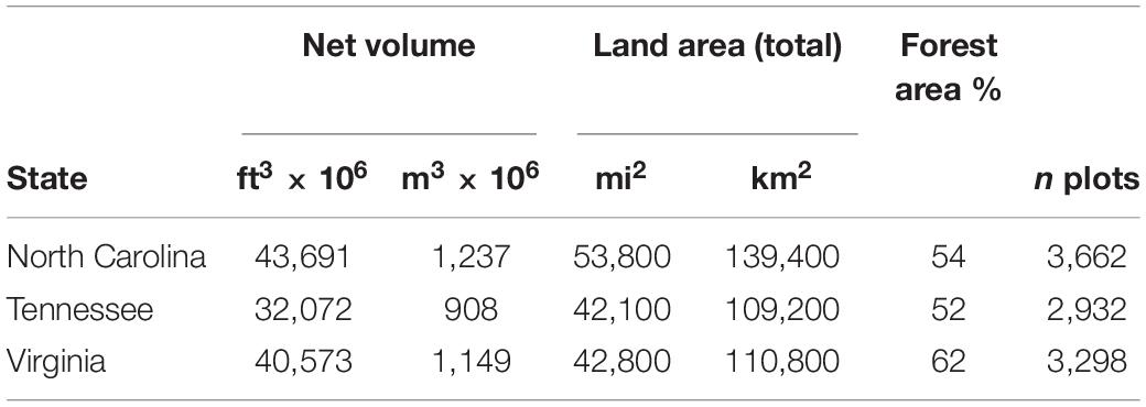
Table 1. Forest volume and land area statistics for states in the study area, with the number of forested FIA sample plots (n) in each state.

Direct estimates of forest volume were obtained using the USDA Forest Service FIA program’s database of field plot measurements for the United States’ NFI (USDA Forest Service FIA, 2021). Estimates were based on the FIA calendar year 2017 forest evaluation, so that full-panel estimates—those based on complete sample sets of field plot measurements collected over 5 years (2015–2019)—were available for estimation (Bechtold and Patterson, 2005). Sampled plot-level data were processed to produce timber volume estimates and standard errors for each county in the three states. The estimated volumes and their standard errors provided direct estimates of forest inventory to be tested for possible precision gains using SAE techniques. The attribute of interest estimated for each county was the total (net) wood volume in live tree main stems having diameters at breast height ≥12.7 cm (i.e., 5.0 inches). The volume attribute excluded wood contents in stumps below a 30.5 cm (1 foot) height, and topwood above a 10.2 cm (4 inch) upper stem diameter.

Auxiliary Data

Digital data in the form of CHM acquired through USDA NAIP served as source of auxiliary information for the SAE analyses. The data were delivered as digital surface model (DSM) raster files having grid cells of approximately 1 × 1 m (TN) and 5 × 5 m (NC and VA) produced from aerial imagery and 3d DAP methods (Strunk et al., 2020). The DSM data were resampled at 10 m × 10 m resolution for overlay with United States National Elevation Database Digital Elevation Model (DEM) data. CHMs were calculated by subtracting DEM values from the NAIP DSMs, setting any negative values to zero.

Land cover data from the National Land Cover Database were used to remove CHM data for raster cells classified as open water. No accounting was made for other land cover types, as the goal was to use auxiliary information derived as much as possible from the NAIP imagery, rather than depending on land cover or vegetation type classifiers derived from other auxiliary sources. The CHM raster layers were clipped to each county boundary and aggregated into seven 5-m interval height classes spanning, {(0, 5), (5, 10), …, (30–35) m}, with values >35 m omitted to remove possible outliers, anomalies, or atmospheric interference, assuming nearly all forest canopies in the study area were ≤35 m in height. County areas covered by each of the seven height classes were calculated as the product of grid cell counts and the cell area in km².

Area-Level Fay-Herriot Model

The area-level approach introduced by Fay and Herriot (1979) and implemented in the R package “sae” (Molina and Marhuenda, 2015) was adopted for conducting SAE analysis. The FH approach uses a composite of two estimates that results in empirically best linear unbiased predictions (EBLUP) of an attribute of interest in each spatial domain. Counties were the domains, and total volumes the attributes of interest here, with the population attribute for a given county (d) denoted as (τ_d). The composite estimator averaged direct and synthetic estimates to produce EBLUPS

${\widehat{\mathrm{\tau }}}_d^{EBLUP}={\widehat{\mathrm{\gamma }}}_d{\widehat{\mathrm{\tau }}}_d^{\text{DIR}}+\left(1-{\widehat{\mathrm{\gamma }}}_d\right)X_d^T\widehat{\mathrm{\beta }}(1)$

where ${\widehat{\mathrm{\tau }}}_d^{\text{DIR}}$ is the direct inventory estimate of total volume for the d^th county, X_d is a vector of canopy height class areas for the county, $\widehat{\mathrm{\beta }}$ is a set of linear regression coefficients estimated from all county-level observations, and the composite weighting factor, i.e., shrinkage ${\widehat{\mathrm{\gamma }}}_d$ is defined as

${\widehat{\mathrm{\gamma }}}_d=\frac{{\widehat{\mathrm{\sigma }}}_a^2}{({\widehat{\mathrm{\sigma }}}_a^2+\widehat{v}({\widehat{\mathrm{\tau }}}_d^{\text{DIR}}))}(2)$

where v denotes the direct estimator variance and ${\widehat{\mathrm{\sigma }}}_a^2$ is the estimated variance among the county totals, formulated as mixed effects in the FH model. A basic idea of the FH estimator and composite estimators used in SAE in general is that the weighting factor provides a way to balance the information between the direct ${\widehat{\mathrm{\tau }}}_d^{\text{DIR}}$ and regression-synthetic $X_d^T\widehat{\mathrm{\beta }}$ estimators. In (1) the weighting factor (2) accounts for relative sizes of the domain-direct variance $\widehat{v}({\widehat{\mathrm{\tau }}}_d^{\text{DIR}})$ and variance among counties measured by the random effect variance ${\widehat{\mathrm{\sigma }}}_a^2$. Parameter estimation, including mixed-effects coefficients and variances approximated by a polynomial expansion, were estimated using restricted maximum likelihood in the “sae” package. Additional details of the estimation procedure are given by Molina and Marhuenda (2015).

Spatial Fay-Herriot Model

A spatial FH model (SFH) was also used to account for possible spatial correlation among estimates from adjacent pairs of counties (Petrucci and Salvati, 2006). The SFH model is built on a FH model with simultaneously autoregressive spatial correlation structure specified by a single parameter ρ and (d × d) proximity matrix W having zero diagonals and ones in off-diagonal elements indexing pairs of adjacent counties, i.e., those that share a common border (Molina and Marhuenda, 2015). The advantage of this spatial model in settings where forest conditions are more alike among adjacent counties than for counties separated by some distance is that it should provide additional precision gains beyond those of the non-spatial FH model.

Model Fitting

In the “sae” package, FH EBLUPS and their mean-squared errors are estimated by functions named eblupFH and mseFH with the response variable specified as the vector of county-level direct estimates of forest volume from FIA sample data, i.e., ${\widehat{\mathrm{\tau }}}_d^{\text{DIR}}$ (10⁶ m³). County-level estimator variances $\widehat{v}({\widehat{\mathrm{\tau }}}_d^{\text{DIR}})$ were given as inputs to the fitting procedure for use in calculating domain weights for use in the composite estimator (1). County-level area coverage (km²) for each canopy height class were specified as predictors, with the full set of predictors including all seven height classes. A zero intercept was found to be supported for the base fixed-effects model based on increased AIC by >2 units when a global intercept was included, with additive random effects estimated for counties. The same inputs were used in fitting the SFH model, but with the proximity matrix also specified.

Both FH and SFH models were fitted with the response formulated as ${\widehat{\mathrm{\mu }}}_d^{\text{DIR}}$, where μ = county volume per unit land area (m³ km^–2) along with a suitable set of predictors that gave roughly equivalent model results, but on a per area basis rather than for county totals. Scaling the predictors to the same per area basis as μ was necessary to preserve the strength of the relationship between response and predictors. Preliminary analyses indicated no meaningful differences in any of the results or hypotheses tested, including comparison of spatial autocorrelations with the SFH method. As a result, only results for totals are reported here.

As in any multiple regression analysis, the correct specification of predictors was investigated, in part to reduce any effects of co-varying predictors that might inflate the estimated variances of regression coefficients. Using a backward elimination procedure based on the greatest reduction in the Akaike Information Criterion (AIC) predictors were sequentially removed from a reference model having a full set of p = 7 predictors, dropping one predictor at a time until AIC was no longer reduced upon removing another predictor. As a further restriction to address a tendency of AIC to select models that are overspecified, we adopted a type-I error rate α = 0.01 for model coefficients to be included in final models. Predictors that did not meet this criterion were dropped from final models.

Apparent Sample Size

A simple formulation for the standard error of a population total estimated from sample observations of the total y, assuming random sampling and ignoring any finite population correction, is ${\widehat{\mathrm{\sigma }}}_{\widehat{\mathrm{\tau }}}={\widehat{\mathrm{\sigma }}}_y/\sqrt{n}$. Using this formula and comparing domain-direct estimated standard errors to RMSEs of EBLUPS obtained from a FH or SFH estimation gave the apparent sample size formula

$n_{app}=n_{for}\times {\left[\frac{{\widehat{\mathrm{\sigma }}}_{\widehat{\mathrm{\tau }}}^{DIR}}{{\widehat{\mathrm{\sigma }}}_{\widehat{\mathrm{\tau }}}^{EBLUP}}\right]}^2(3)$

where n_for is the sample size for the number of forested plots involved in the direct estimate of the total, ${\widehat{\mathrm{\sigma }}}_{\widehat{\mathrm{\tau }}}^{\text{DIR}}$ is the standard error of the direct estimate, and ${\widehat{\mathrm{\sigma }}}_{\widehat{\mathrm{\tau }}}^{\text{EBLUP}}$ is the RMSE of the EBLUP estimated FH or SHF total. Although FIA volume estimates include observed zeros on non-forested plots, the same formulation as (3) can be used to calculate apparent sample sizes for both forest and non-forest plots. To avoid redundancy, only the results for n_app of forested plots are presented here.

Single vs. Multiple State Analyses

In both FH and SFH approaches, composite estimators were first developed using data from NC, TN, and VA fitted separately as “individual states,” effectively treating them as distinct populations for purposes of county-level forest volume estimation. Second, estimators were developed using data from all three states in a single model-fitting procedure, i.e, treating the three “combined states” as a single population divided into county domains. Both approaches produced EBLUP estimates for all counties having at least two FIA sample plots—the minimum needed to estimate the direct estimator variance; however, nothing in the two analyses explicitly constrained the resulting estimates to agree between individual and combined state approaches. Performing separate analyses for each state would lead to three sets of fixed effects coefficients, and three separate random effects variances ${\widehat{\mathrm{\sigma }}}_a^2$, one for each state, compared to just one for the analysis combining the three states. Similarly, the SFH approach gave separate state estimates of ρ for each state, while a single value was estimated in the combined approach.

Evaluation of Spatial Autocorrelation

To compare the FH models to the SFH models we used Likelihood ratio tests (LRT)

$\text{LRT}=2(\text{ln}{L}_1-\text{ln}{L}_2)$

where L₁ and L₂ are the restricted likelihoods calculated for SFH (L₁) and FH (L₂) models, identical except for the correlation parameter ρ. Under the null hypothesis SFH does not improve on the fit of the non-spatial FH model, and large values of the test statistic LRT∼χ²(1) provide evidence for concluding that the SFH model improves on the fit over the FH model.

Estimator Errors

Uncertainty of area-level FH EBLUPs is assessed by mean square error (MSE), calculated in the mseFH R function as an additive combination of terms representing uncertainties associated with (a) prediction of random effects, (b) estimation of regression model coefficients, and (c) estimation of the random-effect variance, i.e., the variance among small-area domains (Prasad and Rao, 1990; Molina and Marhuenda, 2015). The MSE calculation is an second-order approximation using Taylor linearization, shown to be approximately unbiased for large D. Approximate unbiasedness of the Prasad and Rao (1990) MSE estimator holds when any of three estimation techniques are used, including the package default restricted maximum likelihood (REML) used here. A similar approximation for REML estimation based on the findings of Singh et al. (2005) and implemented in the R package function mseSFH was adopted here for calculating MSE for SFH estimates. Both the FH and SFH MSE estimates are known to be asymptotically unbiased, i.e., any bias approaches zero as D → ∞ (cf. Li and Lahiri, 2010; Coulston et al., 2021).

Precision Gains

To evaluate gains in the precision of FH estimators, we used the relative standard errors (RMSE%) for ${\widehat{\mathrm{\tau }}}_d^{\text{DIR}}$ and ${\widehat{\mathrm{\tau }}}_d^{\text{EBLUP}}$ from FIA sample data and FH models, respectively. The RMSE% to be compared for each county were calculated as

${\text{RMSE}\%}_{\text{EBLUP}}=100*\sqrt{\text{MSE}({\widehat{\mathrm{\tau }}}_d^{\text{EBLUP}})}/{\widehat{\mathrm{\tau }}}_d^{\text{DIR}}$

${\text{RMSE}\%}_{\text{DIR}}=100*\sqrt{\text{Var}({\widehat{\mathrm{\tau }}}_d^{\text{DIR}})}/{\widehat{\mathrm{\tau }}}_d^{\text{DIR}}$

and a unitless standard error ratio (SER) for each county was calculated as

$\text{SER}={\text{RMSE}\%}_{\text{EBLUP}}/{\text{RMSE}\%}_{\text{DIR}}$

Results

Model Fitting

Model fixed effects coefficients values generally increased from lowest to highest with CHM height class, consistent with higher volumes per unit area as would be expected for taller forests (Table 2). A notable exception to this increasing trend was the (20, 25] m height class, which contributed less to predicted volumes per km² than lower height classes in the same models. The (30, 35] m CHM height class was a significant predictor for all states and models, including in the combined 3-state model, and had the largest coefficient estimates in all the models tested. The Virginia estimator was the only one to include a significant fixed-effects coefficient for the lowest (0, 5] m height class, and its small magnitude reflected the low potential for forest volumes in such low canopy heights, being less than half the size of the next smallest coefficient value estimated for any model or height class (Table 2).

TABLE 2

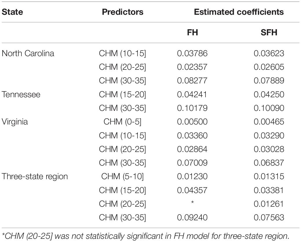
Table 2. Estimated coefficients (10⁶ m³/km²) for best SAE area-level models (p < 0.01 for reported model coefficients).

Best models for individual state estimators included between 2 and 4 predictors, with variable selection excluding predictors for at least one 5-m height class between any two consecutive height classes kept in the final models (Table 2). In the combined three-state spatial model, predictors for two consecutive height bins (15, 20] and (20, 25] were both found to be significant (α = 0.01) despite a greater potential for collinearity due to possible overlapping of information in abutting measurement intervals (see Supplementary Material for predictor scatterplot/correlation matrices).

Fixed effects for the FH estimators were generally in line with those of the SFH models for the single-state analyses (Table 2). Differences between FH and SFH estimates for any predictor diverged by less than 3% percent on average (8 of 9 single-state FH to SFH pairwise comparisons), although a discrepancy of about 11% in magnitude was noted for the NC (20, 25] m height class predictor. Larger differences were noted between the FH and SFH coefficients in the three-state analysis, with differences greater than 18% observed for two height class parameters and the (20, 25] m height class being significantly different from zero in the SFH model but not in the three-state FH model (Table 2). Positive signs on all coefficients suggested that the synthetic models themselves would not produce negative volume estimates, none of which were observed in any of the results produced for the study data.

Spatial vs. Non-spatial Models

Positive spatial autocorrelation estimates for ρ in SFH models (Table 3) indicated that geographically adjacent counties’ forest volumes tended to vary together in the same direction (Griffith, 2005). While LRT did not support the need for the SFH formulation in individual state FH models, the spatial model was found to significantly improve upon the non-spatial FH model in the combined 3-state analysis (Table 3).

TABLE 3

Table 3. Estimated spatial correlation coefficients in SFH models and likelihood ratio tests (LRT) between FH and SFH models.

Precision of Estimation

Comparison of county-level direct estimates to FH EBLUPS showed no obvious inconsistencies that might point to biases in any sets of estimates (Figure 1). Relative RMSE from SAE estimators compared to direct estimate standard errors for county estimates showed magnitudes of reduction in estimator errors (Figure 2). Relative errors for two Virginia counties, Hampton City and Newport News, were noticeably higher (>100%) than the bulk of the state’s counties (Figure 2C). A similarly, high relative error (>80%) was noted for Crockett county, TN (Figure 2B). Volume estimates for all three of these counties were below 28,300 m³ (1 million m³), the smallest three volume estimates of any counties sampled by at least one FIA forest plot in the study. The two Virginia counties—defined by the United States Census Bureau as “county equivalents,” but by the State of Virginia as “independent cities”—had just one FIA forest plot record each, while Crockett County, TN had just two FIA forest plots. No other counties in the study area had fewer than 5 FIA forest sample plots within their boundaries.

FIGURE 1

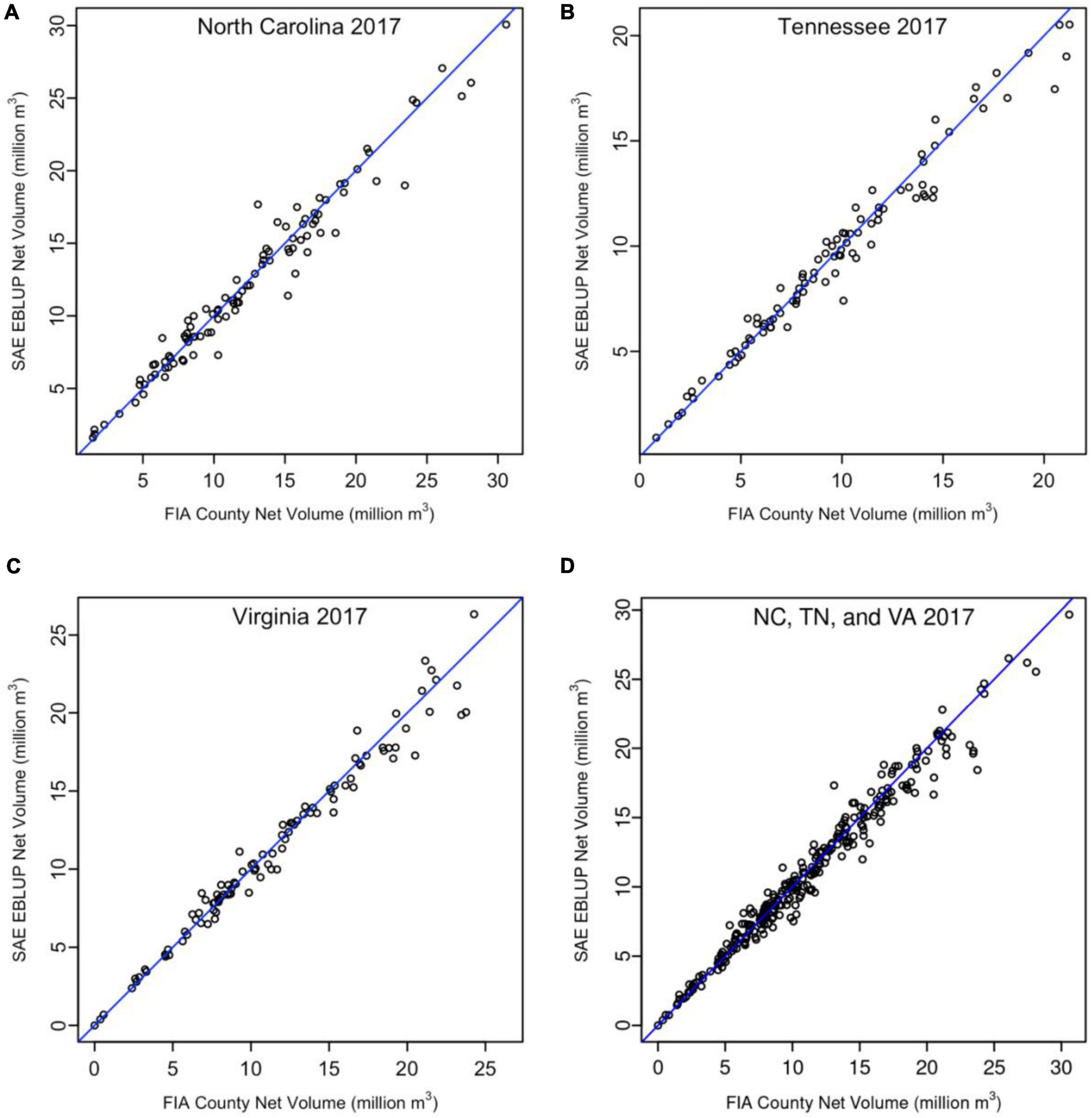
Figure 1. Fay Herriot composite estimates (EBLUP) of county forest volume totals compared to FIA direct estimates for three separate state-level analyses (A–C) and the combined 3-state SFH analysis (D).

FIGURE 2

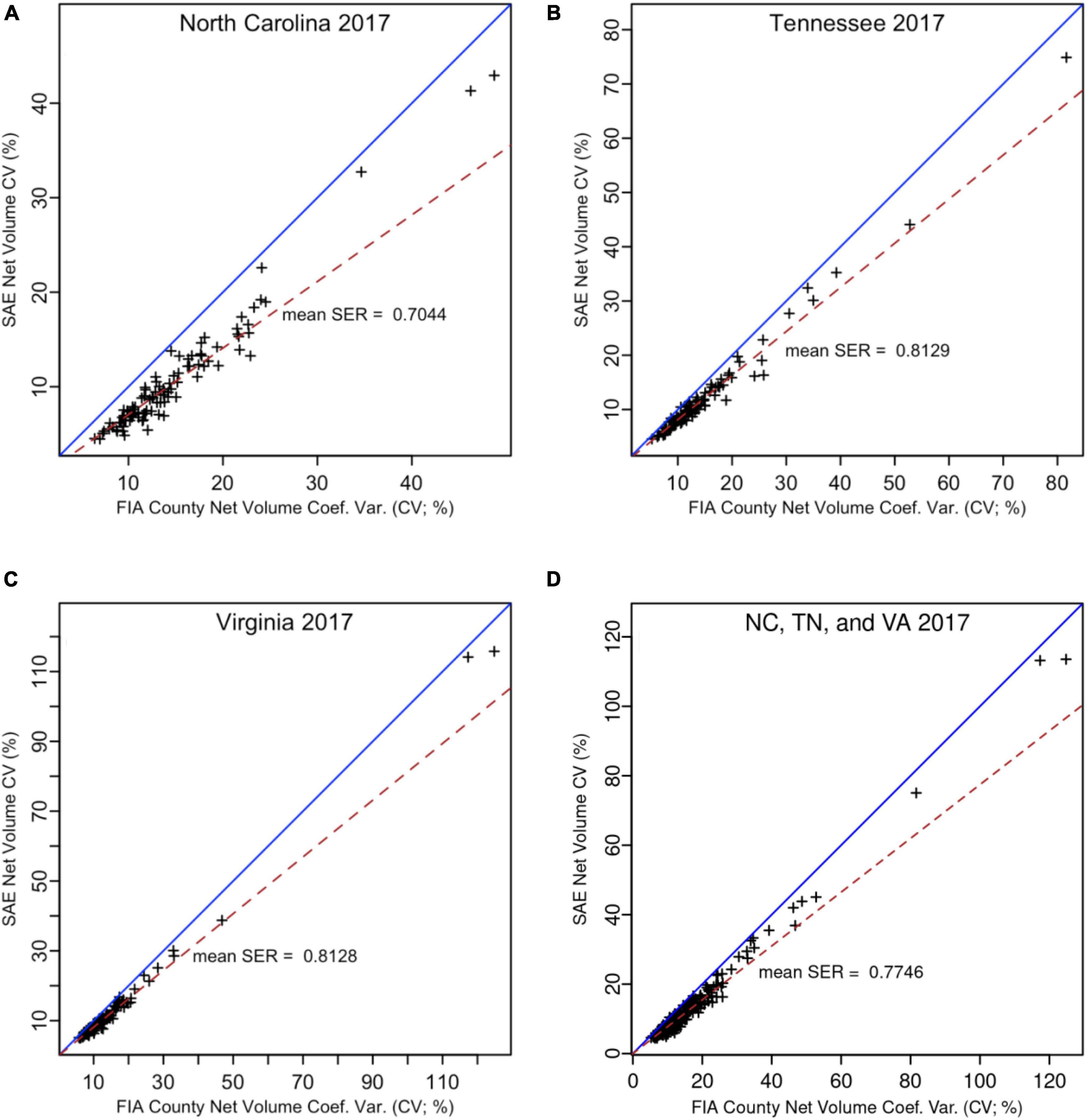
Figure 2. Fay Herriot estimates RMSE% compared to FIA direct estimate standard errors (percent of county total) for three state-level analyses (A–C) and the combined 3-state analysis (D). Non-spatial FH estimators were used for data in panels (A–C), while the SFH estimator was used for panel (D). (note: SER = ratio of standard errors).

Using SER as a measure of the relative reduction in estimator error for each county, North Carolina had the greatest gains in precision at close to a 30% reduction using FH estimators compared to sample domain-direct estimator errors (Table 4 and Figure 2A). Virginia and Tennessee exhibited comparatively modest reductions in estimator errors at about 19% for FH versus direct county estimates (Figures 2B,C).

TABLE 4

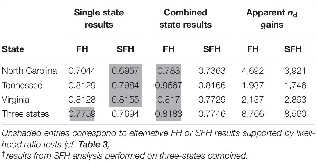
Table 4. Mean standard error ratios (SER) of EBLUP RMSE to direct standard error, averaged over counties within state groupings.

Apparent Sample Size Gains

Apparent sample sizes for each county were calculated by applying (3) to county domains in the study states (Figure 3). Apparent sample size gains for the counties (n_gain = n_app – n_for) attributable to the increased efficiencies of FH estimators were summed for each state and the whole study area to determine roughly how many additional FIA field plots would be required in each state to achieve the county-level precisions afforded by FH and SFH estimators (Table 4). In comparison to the FIA forested plot sample sizes (Table 1), the gains under FH estimation ranged from about 65% in Virginia to about 128% in NC, i.e., more than an apparent doubling of the FIA sample size for forested plots in that state.

FIGURE 3

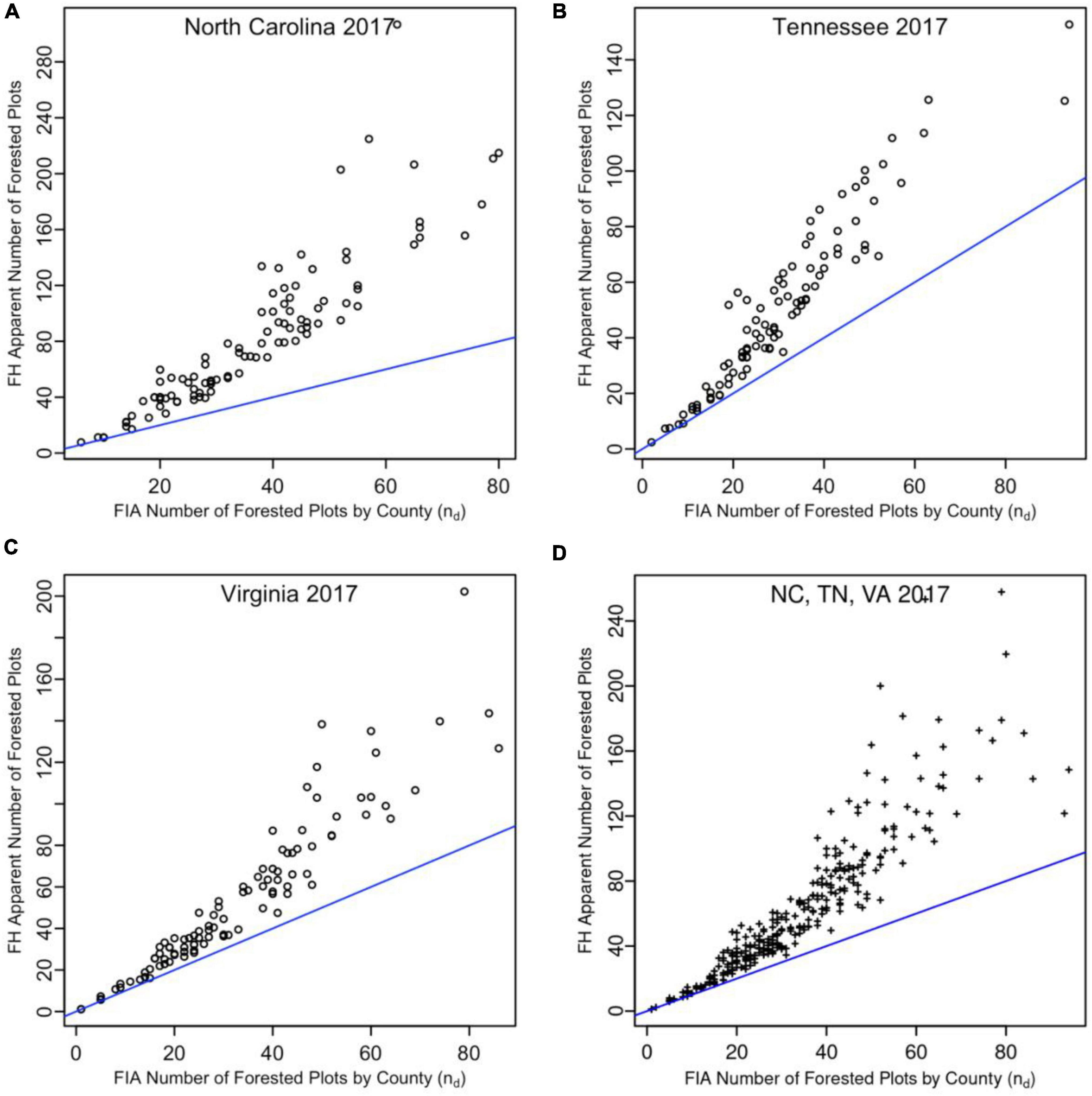
Figure 3. Apparent domain sample sizes (n_d,app) for total forest volume of study area counties compared to FIA sample sizes from direct estimates. Non-spatial FH estimators were used for results shown in panel (A–C), while the SFH estimator was used for panel (D).

Discussion

Reductions in standard errors of direct estimates (volume or biomass) from published studies of area-level SAE vary considerably, from close to zero reduction (SER = 1) for planted pine stands on which relative standard errors of direct estimates were <10% (Green et al., 2020a) to reductions greater than one-half (SER = 0.4) in small natural stands (average 6.1 ha) studied by Ver Planck et al. (2018). Magnussen et al. (2017) achieved considerable error reduction (SER = 0.53) in 25–37 ha management units around Burgos, Spain and Rastatt, Germany, and nearly as good (SER = 0.57) in forest districts and municipalities in Jura canton, Switzerland (70,800 ha) and Vestfold county, Norway (14,900 ha). Breidenbach et al. (2018) attained error reductions (SER = 0.8) similar to what we achieved for TN and VA working with a larger set of domains in Vestfold county than the population studied by Magnussen et al. (2017). While Green et al. (2020a) noted little reduction in standard errors in stands where direct estimates were already quite precise, they showed strong gains (SER = 0.65) in stands having comparatively large uncertainties in direct estimates (up to 30% relative SE). In the states studied here, most counties having direct relative standard errors >30% for total volume did not achieve precision gains as great as their corresponding state averages, i.e., county SERs were not as small as the state average SER (Figure 2). However, such counties comprised a small proportion—about 13 of 295—of the counties studied. Although Goerndt et al. (2013) focused more on domain-specific biases than relative gains in precision, their results showed clearly that gains depended a great deal on the attributes of interest being studied, a consideration not pursued here as we only examined FH model performance in estimating total forest volumes.

Several authors have examined the relationship between sample size and precision gains such as those we measured by SER, as well as the effect of direct estimator precision on SER (Magnussen et al., 2014; Green et al., 2020a). By intentionally reducing domain-specific sample sizes (n_d), Goerndt et al. (2011) demonstrated greatest precision gains (SER = 0.7) for area-based SAE for 2 ≤ n_d ≤ 4. They noted comparatively modest gains (SER > 0.7) for n_d > 4, with no appreciable reduction in variances compared to direct estimates for large samples (n_d > 30). Area-level SAE over a twenty-state region of the northeastern United States involving counties as small-area domains showed gains comparable to those observed in the three-state region studied here, with 0.65 ≤ SER ≤ 0.95 (Goerndt et al., 2019). Despite there being many large sample sizes in the three states we studied—median n_d = 31 (forested plots) and median n_d = 50 (all plots)—SERs for the 295 counties studied here averaged 0.77 (Figure 2D) with SER 2.5th and 97.5th percentiles [0.58, 0.94] (Supplementary Table 1) showing appreciable gains in precision for FH results across all domain-specific (county) sample sizes. Precision gains observed here across a range of forested plots’ sample sizes from 5 ≤ n_d ≤ 96 differ from what other authors have shown, possibly because our analysis did not rely on generalized variance functions, which are known to convey mainly information on n_d, rather than directly estimated within-domain variation (Goerndt et al., 2011; Coulston et al., 2021).

While precision gains were notable for estimating total wood volume with FH EBLUPS compared to direct, design-based estimates, a significant concern is that end-users often require volume estimates disaggregated by forest type or species groups (e.g., hardwoods or softwoods), or by product classes such as pulpwood or sawtimber (Coulston et al., 2021). End-users may also wish to preserve consistency among estimates of multiple attributes for which NFI data provides estimates, including biomass, stem density, basal area, or any of dozens to hundreds of other attributes. While not pursued here, multivariate FH models have been developed and applied to situations where multivariate estimates were sought from repeated sampling (Ghosh et al., 1996; Benavent and Morales, 2016). Model-assisted methods may also allow for simultaneous and compatible estimation of multiple attributes, or generic inference, as distinguished from the focus on a single attribute of interest, or specific inference, pursued here (McRoberts et al., 2017; McConville et al., 2020). Expanding the analyses conducted here to multivariate cases would constitute a significant augmentation.

Accounting for spatial correlation among adjacent counties had minimal effect in single-state analyses conducted here and modest effect in the combined model involving all three states, likely due to a mismatch between the scale at which the counties in this study differed from scales of natural and anthropogenic processes affecting total wood volumes in the states and counties studied. We note that the mean land area of 295 counties studied here was 1,218 km², with a range of [107, 4,047] km² (Supplementary Table 1). The lack of spatial correlation differed from other work that found substantial reductions in SER when spatial autocorrelation was accounted for Magnussen et al. (2014); Ver Planck et al. (2018). Observed gains may be related to the areas of domains studied, such as in relatively small stands studied by Ver Planck et al. (2018), which were necessarily much closer in proximity (e.g., as could be measured by centroid distances) due to their small land areas than the county domains we studied. Closer proximities among domains does not necessarily explain the gains achieved in accounting for spatial correlation noted by Magnussen et al. (2014) in their study of large Swiss forest districts spanning an area of 14,000 km². One result from our combined 3-state analysis that agreed with results of Ver Planck et al. (2018) is that accounting for spatial correlation can increase overall precision when averaged across many small area domains. Our results were also consistent with results presented by Ver Planck et al. (2018) that showed while the SFH reduced relative errors in some domains, it led to increased errors in others. When presented as maps of relative standard errors for counties in the study region (Figures 4, 5), it becomes evident that gains in precision for combining states and using SFH reduced the errors in some counties in Virginia while increasing errors in some counties in North Carolina and Tennessee. Such tradeoffs should be considered when choosing an approach for implementation.

FIGURE 4

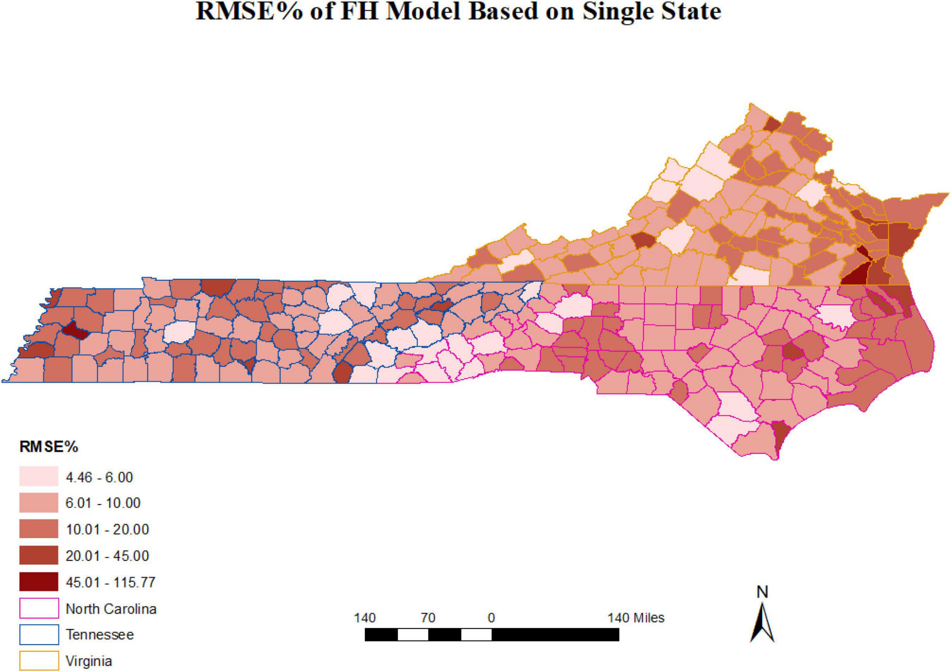
Figure 4. Relative standard errors of non-spatial Fay-Herriot EBLUP estimates of county total forest volume, obtained from separate models for each of three states, North Carolina, Tennessee, and Virginia.

FIGURE 5

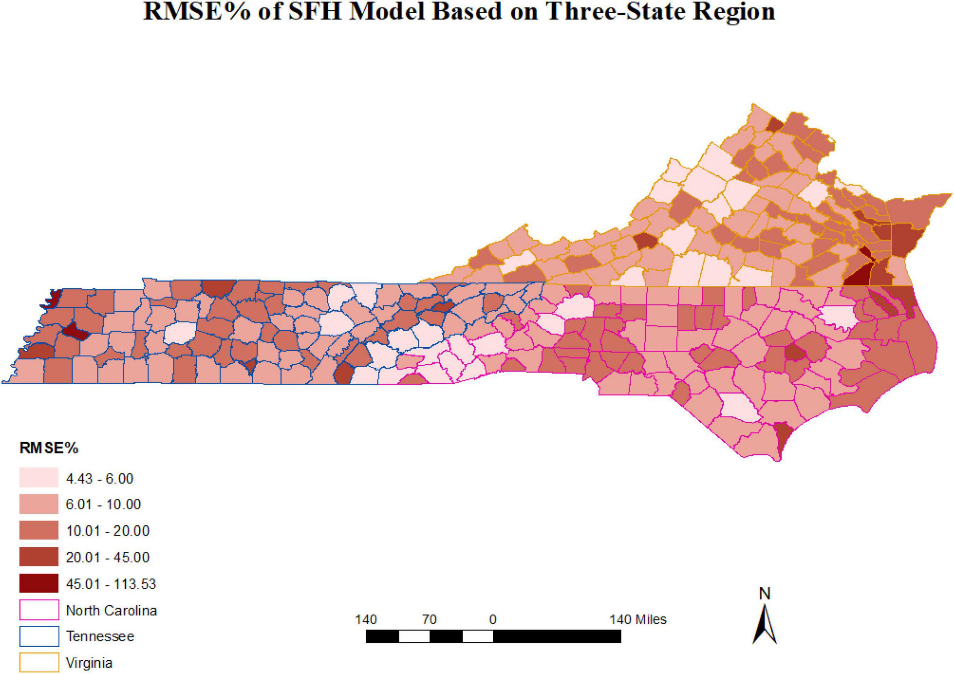
Figure 5. Relative standard errors of simultaneous autoregressive spatial Fay-Herriot EBLUP estimates of county total forest volume obtained from a single model combining data for three states in the southeastern United States.

Since county areas are treated as known, fixed quantities in the FIA estimation framework, scaling of responses, predictors, model coefficients, and estimated RMSEs to a per-area basis can be accomplished post hoc by dividing quantities related to totals by the corresponding county areas (Supplementary Table 1). No recalculation of model parameter estimates, including the spatial correlation parameters in SFH results is necessary. Future work could look at how results generated per unit of forest land might differ from the area totals (or totals scaled per unit area of all land) presented here. Since forest land area is an estimated quantity in the FIA inventory design, estimates per unit of forest land area would consist of ratio estimates with both numerator (volume) and denominator (forest land area) being estimated quantities. It is possible that the spatial correlation structure for such ratio estimates differs from those noted here.

Further gains in estimator efficiency should be possible by including additional auxiliary information to reduce likely inconsistencies in the largely unmodified NAIP CHM information used here (Hansen et al., 2013; Potapov et al., 2020). Apart from filtering CHMs to omit areas over water, no efforts were made here to eliminate pixels in the CHMs representing heights of vegetation or other structures lying outside of areas that would typically be classified as forestland in the FIA inventory. Features such as buildings or other raised structures, urban forests, small patches of trees growing outside of areas defined as forest (see Glossary of Terms, Bechtold and Patterson, 2005), agricultural crops, or features in other land types undoubtedly contributed to the summed canopy height class metrics derived from CHM metrics used as predictors in the synthetic models developed here (Hansen et al., 2016). Although the current study was focused on gains to be realized with minimal processing of NAIP CHMs as-delivered, exploring the impact of non-forest features on forest volume estimates is a topic of considerable interest (Potapov et al., 2021).

Cost Effectiveness

Results of this work demonstrated the magnitudes of gains in efficiency possible by integrating NAIP-derived CHMs with direct sample data from NFI field plots using the area-level FH and SFH procedures. Such information can be used to evaluate cost-effectiveness of implementing the approach to other states or repeating a NAIP 3d acquisition at a future date, such as in monitoring forest growing stock change over time. In considering this, we defined the costs of collecting sample data from a single survey plot (C_plot) and the cost of acquiring NAIP 3d DAP coverage for a state (C_NAIP).

The cost of additional forest plots needed in direct estimation to attain the same level of precision that SAE analysis using NAIP CHM data provided is C_plot × n_gain, leading to the following cost effectiveness (C_e) calculation

$C_e=\frac{C_{\text{NAIP}}}{C_{\text{plot}}\times n_{\text{gain}}}$

where values of C_e < < 1 should indicate some degree of cost-effectiveness for acquiring NAIP 3d imagery. In the three states studied here, the inequality C_e < 1 requires a cost ratio C_NAIP/C_plot < n_gain, with values of n_gain ranging from 1,937 to 4,692 (Table 4). From this basic calculation, it appears that NAIP acquisition costs below about 2,000 times the cost of adding an additional sample plot measurement would be worth considering for states like North Carolina, Tennessee, or Virginia, at least from the perspective of cost-effectiveness. In actual settings, cost considerations would not likely be this simple. For instance, when evaluating a decision to install new field plots, potential costs would undoubtedly be different than the cost of remeasuring existing plots. Other factors such as the number of plots and forest acreage in states would also merit consideration.

Precision Standards

Direct and SAE estimates of precision in this study can shed light on the degree to which the FIA standard for precision could be met or exceeded using FH type estimators. Because the estimates in this study are for all forest land, rather than limited to commercial forest land, the 5% standard may not be representative of FIA direct estimates’ precision, despite approaching the 5% standard (Figure 6). Even so, gains achieved using SAE demonstrate that the standard can be met at a smaller volume threshold, perhaps 90% of the current 1 billion ft³ by incorporating photogrammetric CHM information into estimates (Figure 6).

FIGURE 6

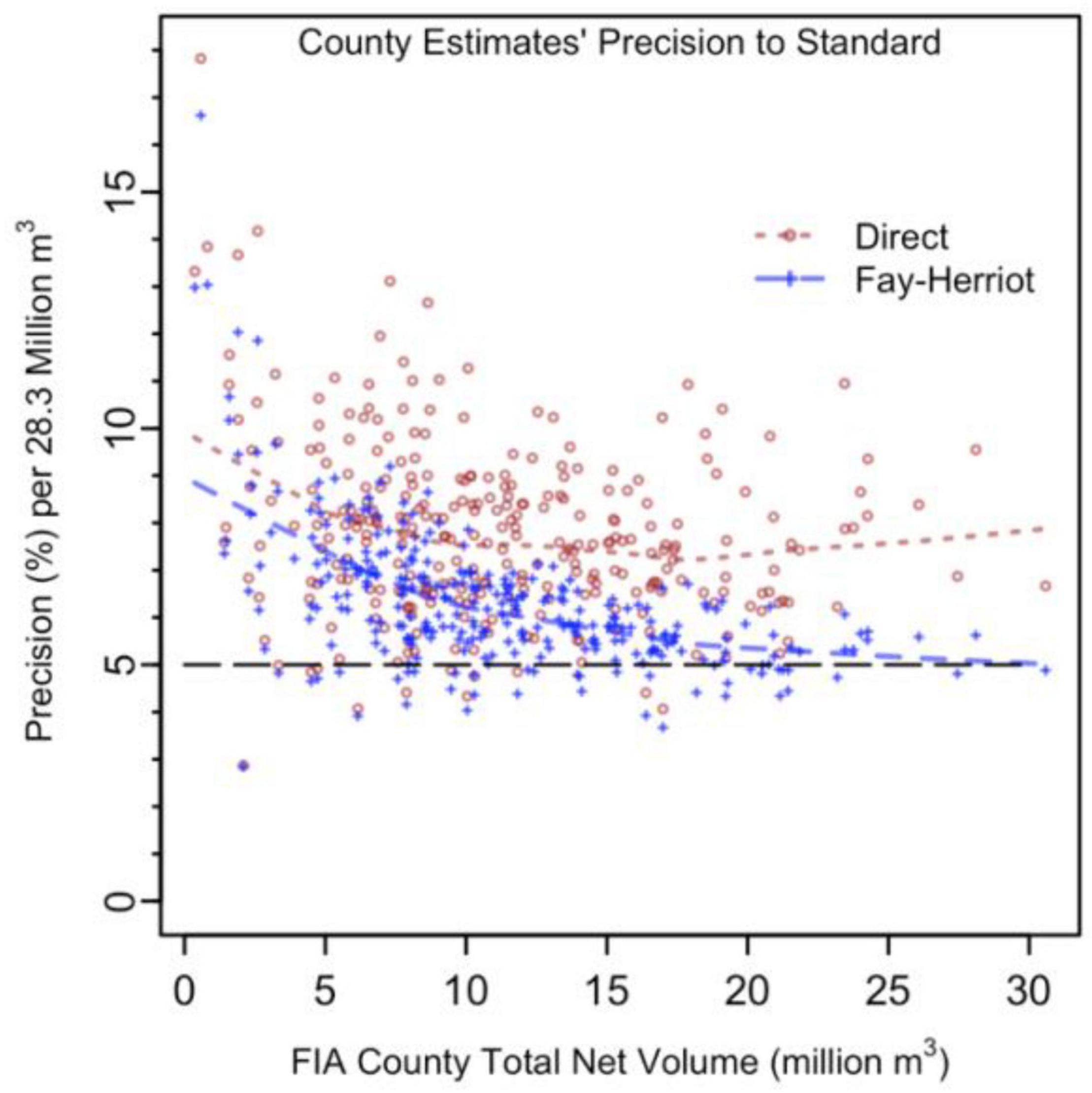
Figure 6. Relative standard errors of FIA direct and FH county forest volume estimates (million m³) with 5% precision standard per 28.3 million m³.

Conclusion

Area-level SAE models using NAIP 3d DAP canopy heights as auxiliary information provided precision gains averaging between 19 and 30% for estimates of county-level forest volumes in North Carolina, Tennessee, and Virginia, compared to estimates made from FIA sample data alone. Choosing the appropriate populations from which to generate county-level FH estimates, i.e., using single states or combining data from multiple states, should be given due consideration in operational inventory settings. The applied research presented here is the first example we know of that applied SAE techniques to FIA survey data at state and county-level scales, which should make results relevant to stakeholders concerned with increasing efficiencies in FIA inventory estimation. Results suggest that the non-spatial model seemed adequate in generating county-level estimates in single-state settings, while the area-level model accounting for spatial autocorrelation was better suited in the combined three-state setting. Composite FH-type area-level estimators showed high potential for increasing precision in county-level estimates of growing stock volume with considerable gains in apparent sample sizes, a clear measure of cost-effectiveness, and seemingly little or no added bias. Further examination of potential gains in estimating other forest attributes in the FIA program—including measuring change over time–seem warranted, as do the use of other sources of auxiliary information and the application of these methods to other states and regions in the United States.

Data Availability Statement

The original contributions presented in the study are included in the article/Supplementary Material, further inquiries can be directed to the corresponding author.

Author Contributions

QC and GD: analysis and principal authorship. PR: research planning, analysis, and principal authorship. JC: project coordination, research planning, analysis, and co-authorship. JD: analysis and technical consultation. VT: research planning and scientific consultation. HB: scientific consultation and co-authorship. RW: project coordination and research planning. All authors contributed to the article and approved the submitted version.

Funding

This work was supported by USDA, Forest Service Southern Research Station, 20-JV-11330145-074.

Conflict of Interest

The authors declare that the research was conducted in the absence of any commercial or financial relationships that could be construed as a potential conflict of interest.

Publisher’s Note

All claims expressed in this article are solely those of the authors and do not necessarily represent those of their affiliated organizations, or those of the publisher, the editors and the reviewers. Any product that may be evaluated in this article, or claim that may be made by its manufacturer, is not guaranteed or endorsed by the publisher.

Supplementary Material

The Supplementary Material for this article can be found online at: https://www.frontiersin.org/articles/10.3389/ffgc.2022.769917/full#supplementary-material

References

Battese, G. E., Harter, R. M., and Fuller, W. A. (1988). An error-components model for prediction of county crop areas using survey and satellite data. J. Am. Stat. Assoc. 83, 28–36. doi: 10.1080/01621459.1988.10478561

CrossRef Full Text | Google Scholar

Bechtold, W. A., and Patterson, P. L. (2005). The Enhanced Forest Inventory and Analysis Program – National Sampling Design and Estimation Procedures. Gen. Tech. Rep. SRS-80. Asheville, NC: U.S. Department of Agriculture, Forest Service, Southern Research Station, 85.

Google Scholar

Benavent, R., and Morales, D. (2016). Multivariate Fay–Herriot models for small area estimation. Comput. Stat. Data Anal. 94, 372–390. doi: 10.1016/j.csda.2015.07.013

CrossRef Full Text | Google Scholar

Breidenbach, J., and Astrup, R. (2012). Small area estimation of forest attributes in the Norwegian National Forest Inventory. Eur. J. For. Res. 131, 1255–1267. doi: 10.1007/s10342-012-0596-7

CrossRef Full Text | Google Scholar

Breidenbach, J., Magnussen, S., Rahlf, J., and Astrup, R. (2018). Unit-level and area-level small area estimation under heteroscedasticity using digital aerial photogrammetry data. Remote Sens. Environ. 212, 199–211. doi: 10.1016/j.rse.2018.04.028

CrossRef Full Text | Google Scholar

Brosofske, K. D., Froese, R. E., Falkowski, M. J., and Banskota, A. (2014). A review of methods for mapping and prediction of inventory attributes for operational forest management. For. Sci. 60, 733–756. doi: 10.5849/forsci.12-134

CrossRef Full Text | Google Scholar

Coulston, J. W., Green, P. C., Radtke, P. J., Prisley, S. P., Brooks, E. B., Thomas, V. A., et al. (2021). Enhancing the precision of broad-scale forestland removals estimates with small area estimation techniques. For. Int. J. For. Res. 94, 427–441. doi: 10.1093/forestry/cpaa045

CrossRef Full Text | Google Scholar

Fay, R. E., and Herriot, R. A. (1979). Estimates of Income for small places: an application of James-Stein procedures to census data. J. Am. Stat. Assoc. 74, 269–277. doi: 10.2307/2286322

CrossRef Full Text | Google Scholar

Fuller, W. A. (1999). Environmental surveys over time. J. Agric. Biol. Environ. Stat. 4, 331–345. doi: 10.2307/1400493

CrossRef Full Text | Google Scholar

Ghosh, M., Nangia, N., and Kim, D. H. (1996). Estimation of median income of four-person families: a Bayesian time series approach. J. Am. Stat. Assoc. 91, 1423–1431. doi: 10.1080/01621459.1996.10476710

CrossRef Full Text | Google Scholar

Goerndt, M. E., Monleon, V. J., and Temesgen, H. (2011). A comparison of small-area estimation techniques to estimate selected stand attributes using LiDAR-derived auxiliary variables. Can. J. For. Res. 41, 1189–1201. doi: 10.1139/x11-033

CrossRef Full Text | Google Scholar

Goerndt, M. E., Monleon, V. J., and Temesgen, H. (2013). Small-area estimation of county-level forest attributes using ground data and remote sensed auxiliary information. For. Sci. 59, 536–548. doi: 10.5849/forsci.12-073

CrossRef Full Text | Google Scholar

Goerndt, M. E., Wilson, B. T., and Aguilar, F. X. (2019). Comparison of small area estimation methods applied to biopower feedstock supply in the Northern U.S. region. Biomass Bioenergy 121, 64–77. doi: 10.1016/j.biombioe.2018.12.008

CrossRef Full Text | Google Scholar

Green, P. C., Burkhart, H. E., Coulston, J. W., and Radtke, P. J. (2020a). A novel application of small area estimation in loblolly pine forest inventory. Forestry 93, 444–457. doi: 10.1093/forestry/cpz073

CrossRef Full Text | Google Scholar

Green, P. C., Burkhart, H., Coulston, J., Radtke, P., and Thomas, V. A. (2020b). Auxiliary information resolution effects on small area estimation in plantation forest inventory. Forestry 93, 685–693. doi: 10.1093/forestry/cpaa012

CrossRef Full Text | Google Scholar

Griffith, D. A. (2005). Effective geographic sample size in the presence of spatial autocorrelation. Ann. Assoc. Am. Geogr. 95, 740–760. doi: 10.1111/j.1467-8306.2005.00484.x

CrossRef Full Text | Google Scholar

Hansen, M. C., Potapov, P. V., Goetz, S. J., Turubanova, S., Tyukavina, A., Krylov, A., et al. (2016). Mapping tree height distributions in Sub-Saharan Africa using Landsat 7 and 8 data. Remote Sens. Environ. 185, 221–232. doi: 10.1016/j.rse.2016.02.023

CrossRef Full Text | Google Scholar

Hansen, M. C., Potapov, P. V., Moore, R., Hancher, M., Turubanova, S. A., Tyukavina, A., et al. (2013). High-resolution global maps of 21st-century forest cover change. Science 342, 850–853. doi: 10.1126/science.1244693

PubMed Abstract | CrossRef Full Text | Google Scholar

Lehtonen, R., and Veijanen, A. (2009). “Chapter 31 — Design-based methods for domains and small areas,” in Handbook of Statistics 29B Sample Surveys : Inference and Analysis, eds D. Pfefferman and C. R. Rao (Amsterdam: Elsevier), 219–249. doi: 10.1016/s0169-7161(09)00231-4

CrossRef Full Text | Google Scholar

Li, H. L., and Lahiri, P. (2010). An adjusted maximum likelihood method for solving small area estimation problems. J. Multiv. Anal. 101, 882–892. doi: 10.1016/j.jmva.2009.10.009

PubMed Abstract | CrossRef Full Text | Google Scholar

Magnussen, S., Mandallaz, D., Breidenbach, J., Lanz, A., and Ginzler, C. (2014). National forest inventories in the service of small area estimation of stem volume. Can. J. Res. 44, 1079–1090. doi: 10.1139/cjfr-2013-0448

CrossRef Full Text | Google Scholar

Magnussen, S., Mauro, F., Breidenbach, J., Lanz, A., and Kändler, G. (2017). Area-level analysis of forest inventory variables. Eur. J. For. Res. 136, 839–855. doi: 10.1371/journal.pone.0189401

PubMed Abstract | CrossRef Full Text | Google Scholar

Mauro, F., Molina, I., García-Abril, A., Valbuena, R., and Ayuga-Téllez, E. (2016). Remote sensing estimates and measures of uncertainty for forest variables at different aggregation levels. Environmetrics 27, 225–238. doi: 10.1002/env.2387

CrossRef Full Text | Google Scholar

Mauro, F., Monleon, V. J., Temesgen, H., and Ford, K. R. (2017). Analysis of area level and unit level models for small area estimation in forest inventories assisted with LiDAR auxiliary information. PLoS One 12:e0189401. doi: 10.1371/journal.pone.0189401

PubMed Abstract | CrossRef Full Text | Google Scholar

Mauro, F., Ritchie, M., Wing, B., Frank, B., Monleon, V., Temesgen, H., et al. (2019). Estimation of changes of forest structural attributes at three different spatial aggregation levels in northern California using multitemporal LiDAR. Remote Sens. 11:293.

Google Scholar

McConville, K. S., Moisen, G. G., and Frescino, T. S. (2020). A tutorial on model-assisted estimation with application to forest inventory. Forests 11:244. doi: 10.3390/f11020244

CrossRef Full Text | Google Scholar

McRoberts, R. E. (2012). Estimating forest attribute parameters for small areas using nearest neighbors techniques. For. Ecol. Manag. 272, 3–12. doi: 10.1016/j.foreco.2011.06.039

CrossRef Full Text | Google Scholar

McRoberts, R. E., Chen, Q., and Walters, B. F. (2017). Multivariate inference for forest inventories using auxiliary airborne laser scanning data. For. Ecol. Manag. 401, 295–303. doi: 10.1016/j.foreco.2017.07.017

CrossRef Full Text | Google Scholar

Molina, I., and Marhuenda, Y. (2015). sae: an R package for small area estimation. R J. 7, 81–98. doi: 10.32614/rj-2015-007

CrossRef Full Text | Google Scholar

Petrucci, A., and Salvati, N. (2006). Small area estimation for spatial correlation in watershed erosion assessment. J. Agric. Biol. Environ. Stat. 11, 169–182. doi: 10.1198/108571106x110531

PubMed Abstract | CrossRef Full Text | Google Scholar

Potapov, P., Hansen, M. C., Kommareddy, I., Kommareddy, A., Turubanova, S., Pickens, A., et al. (2020). Landsat analysis ready data for global land cover and land cover change mapping. Remote Sens. 12:426. doi: 10.3390/rs12030426

CrossRef Full Text | Google Scholar

Potapov, P., Li, X., Hernández-Serna, A., Tyukavina, A., Hansen, M. C., Kommareddy, A., et al. (2021). Mapping global forest canopy height through integration of GEDI and Landsat data. Remote Sens. Environ. 253:112165. doi: 10.1016/j.rse.2020.112165

CrossRef Full Text | Google Scholar

Prasad, N. G. N., and Rao, J. N. K. (1990). The estimation of the mean squared error of small-area estimators. J. Am. Stat. Assoc. 85, 163–171. doi: 10.1080/01621459.1990.10475320

CrossRef Full Text | Google Scholar

Rao, J. N. K., and Molina, I. (2015). Small Area Estimation. Hoboken, NJ: John Wiley & Sons, 480.

Google Scholar

Reams, G. A., Roesch, F. A., and Cost, N. D. (1999). Annual forest inventory: cornerstone of sustainability in the south. J. For. 97, 21–26.

Google Scholar

Reich, R. M., and Aguirre-Bravo, C. (2009). Small-area estimation of forest stand structure in Jalisco, Mexico. J. For. Res. 20, 285–292. doi: 10.1007/s11676-009-0050-y

CrossRef Full Text | Google Scholar

Singh, B. B., Shukla, G. K., and Kundu, D. (2005). Spatio-temporal models in small area estimation. Survey Methodol. 31, 183–195.

Google Scholar

Strunk, J. L., Gould, P. J., Packalen, P., Gatziolis, D., Greblowska, D., Maki, C., et al. (2020). Evaluation of pushbroom DAP relative to frame camera DAP and lidar for forest modeling. Remote Sens. Environ. 237:111535. doi: 10.1016/j.rse.2019.111535

CrossRef Full Text | Google Scholar

USDA Forest Service National Headquarters (2008). “Chapter 10 – Operational procedures,” in Forest Survey Handbook. FSH 4809.11_10 (Washington, DC: U.S. Department of Agriculture, Forest Service).

Google Scholar

USDA Forest Service FIA (2021). Forest Inventory and Analysis Database. St. Paul, MN: U.S. Department of Agriculture, Forest Service, Northern Research Station.

Google Scholar

Ver Planck, N. R., Finley, A. O., Kershaw, J. A. Jr., Weiskittel, A. R., and Kress, M. C. (2018). Hierarchical Bayesian models for small area estimation of forest variables using LiDAR. Remote Sens. Environ. 204, 287–295. doi: 10.1016/j.rse.2017.10.024

CrossRef Full Text | Google Scholar

Wang, H.-J., Prisley, S. P., Radtke, P. J., and Coulston, J. W. (2011). Errors In terrain-based model predictions caused by altered forest inventory plot locations in the Southern Appalachian Mountains, USA. Math. Comput. For. Nat. Resour. Sci. 3, 114–123.

Google Scholar