 Chris J. Peterson
 Jeffery B. Cannon
94% of researchers rate our articles as excellent or good
Learn more about the work of our research integrity team to safeguard the quality of each article we publish.
Find out more
ORIGINAL RESEARCH article
Front. For. Glob. Change, 23 December 2021
Sec. Forest Disturbance
Volume 4 - 2021 | https://doi.org/10.3389/ffgc.2021.719813
This article is part of the Research TopicLiving with Tropical Storms in a Changing ClimateView all 6 articles
Tree damage from a variety of types of wind events is widespread and of great ecological and economic importance. In terms of areas impacted, tropical storms have the most widespread effects on tropical and temperate forests, with southeastern U.S. forests particularly prone to tropical storm damage. This impact motivates attempts to understand the tree and forest characteristics that influence levels of damage. This study presents initial findings from a spatially explicit, individual-based mechanistic wind severity model, ForSTORM, parameterized from winching research on trees in southeastern U.S. This model allows independent control of six wind and neighborhood parameters likely to influence the patterns of wind damage, such as gap formation, the shape of the vertical wind profile, indirect damage, and support from neighbors. We arranged the subject trees in two virtual stands orientations with identical positions relative to each other, but with one virtual stand rotated 90 degrees from the other virtual stand – to explore the effect of wind coming from two alternative directions. The model reproduces several trends observed in field damage surveys, as well as analogous CWS models developed for other forests, and reveals unexpected insights. Wind profiles with higher extinction coefficients, or steeper decrease in wind speed from canopy top to lower levels, resulted in significantly higher critical wind speeds, thus reducing level of damage for a given wind speed. Three alternative formulations of wind profiles also led to significant differences in critical wind speed (CWS), although the effect of profile was less than effect of different extinction coefficients. The CWS differed little between the two alternative stand orientations. Support from neighboring trees resulted in significantly higher critical wind speeds, regardless of type of wind profile or spatial arrangement of trees. The presence or absence of gaps caused marginally significant different in CWS, while inclusion of indirect damage along with direct damage did not significantly change CWS from those caused by direct damage alone. Empirical research that could most benefit this modelling approach includes improving crown area measurement, refining drag coefficients, and development of a biomechanical framework for neighbor support.
Tropical storms are a widespread phenomenon that affect widely differing forests on the eastern coast of North America, both coasts of Central America, southwest Africa and Madagascar, the Indian subcontinent, and throughout southeast Asia and nearby Australasia. In the southeastern U.S., tropical storms are the dominant type of forest wind disturbance, although these forests are also subject to tornadoes, derechos, thunderstorm squall lines, and even mountain bora winds (Xi and Peet, 2011; Peterson et al., 2016). The ecological and economic impact of tropical storms can be immense. Hurricane Michael in October of 2018 downed an estimated 500–550 million pine trees in Florida alone, causing $1.3 billion in economic losses; neighboring Georgia, despite being further inland, suffered roughly $750 million in damages (Cassels, 2020). In terms of area impacted, Florida experienced storm damage across 3 million forested acres while an additional 2 million acres were damaged in Georgia (Jackson, 2019). Following catastrophic disturbances, opportunities to recover timber losses through salvage logging can be limited, especially for small landowners (Gordon et al., 2018). Ecological impacts can be equally extreme. Chambers et al. (2007) estimated that the carbon footprint (the amount of tree carbon converted to decomposing by a storm) of Hurricane Katrina in 2005 was roughly equal to the total net annual carbon sink in forest trees of the continental U.S. In the following year, areas hit by Category 3 winds from Katrina experienced a 14% decline in net primary productivity (Ambinakudige and Khanal, 2010). Shifts in community composition are also evident as Xi et al. (2019) found that even moderate hurricanes increase understory species diversity and shift composition to more shade-tolerant species on the North Carolina Piedmont (see also Holzmueller et al., 2012).
These severe ecological and economic impacts provide an impetus to further understanding of tropical storm impacts in forests of the southeastern U.S. Modelling can provide a crucial pathway to such improved understanding, because empirical studies of storm impacts can be difficult, have problems with confounded variables, such as tree species, size and soil type (Rutledge et al., 2021), and may take years to decades to reach fruition (Xi et al.’s 2019 study followed impacts of Hurricane Fran for two decades). In particular, researchers can use models to ask how various storm or forest characteristics influence the levels of damage, and explore how alternative management actions such as various levels of thinning, might affect forest vulnerability to such storms. A variety of modelling approaches have proven fruitful for various objectives, including statistical models (that typically use logistic regression or similar methods; e.g., Peterson, 2007), geographic information systems (GIS) analyses (Zeng et al., 2009; Krejci et al., 2018), and mechanistic models (e.g., GALES and HWIND, Peltola et al., 1999; Gardiner et al., 2000, 2008). More recently, neural network and machine learning modelling approaches have proven themselves powerful tools for estimating tree wind risk (Hart et al., 2019). Fewer attempts have been made to address stand-level phenomenon known to exist. Important factors that influence wind damage, such as indirect damage from larger trees; sheltering from upwind neighbors; and mutual support among neighboring trees, are still absent from stand-level wind damage models. Other damage simulators such as ForGEM (Schelhaas et al., 2007) and iLand (Seidl et al., 2014) include these phenomena but have not been parameterized for southeastern Coastal Plain forests. Moreover, to date, there appear to be few studies that have compared wind profiles or wind attenuation coefficients.
Our goal here is to report on initial efforts to develop a mechanistic modelling tool to generate hypotheses about factors that influence tropical storm damage in southeastern U.S. forests.
We have assembled an individual-based, spatially explicit forest storm damage simulator, called ForSTORM, which allows us to run simulations of wind damage under a wide range of parameter settings, and derive predictions of the critical wind speeds (CWS) that cause damage on a tree-by-tree basis. Numerous CWS studies have explored effects of tree characteristics (e.g., Peltola et al., 1999; Achim et al., 2005; Elie and Ruel, 2005), such as height, age, and allometry, as well as stand characteristics such as spacing and density (Cucchi et al., 2005). Several studies find a greater influence of larger-scale (e.g., stand or landscape scale) characteristics than tree-scale characteristics (Anyomi and Ruel, 2015; Hart et al., 2019; Ruel and Gardiner, 2019), but rarely has research focused on the influence of neighborhood interactions such as sheltering, gaps, indirect damage, and neighbor support. This is despite wide recognition that the localized neighborhood interactions may influence tree failure dynamics; one potential reason for the limited focus on neighborhood interactions is that the model context necessarily must be spatially explicit and individual-based, whereas many CWS studies do not consider tree locations or variation among individuals. Two exceptions are the forest dynamics simulators iLand (Seidl et al., 2014) and ForGEM (Schelhaas et al., 2007), which have both included the above neighborhood interactions in their wind damage modules. Here we attempt to explore the CWS consequences, and associated changes in community metrics, of wind characteristics and neighborhood interactions whose influences are still poorly understood. In this first use of the model, we advance the following tentative hypotheses:
(1). Alternative wind profiles, even when using similar attenuation coefficients, will produce substantially different tree failure dynamics and CWS.
(2). Lower attenuation coefficients allow greater wind penetration and thus lower CWS than higher attenuation coefficients.
(3). Different stand orientations will result in substantial changes in the distribution of CWS.
(4). Inclusion of indirect damage will increase the amount of damage observed at a given wind speed and therefore decrease mean CWS, compared to simulations with direct damage only.
(5). Inclusion of support from neighboring trees will reduce the force that a given tree must withstand and therefore increase CWS, compared to simulations without neighbor support.
(6). The presence of gaps will increase vulnerability of immediate downwind trees, thereby lowering overall CWS.
We will examine the CWS consequences of controlling the above influential factors.
A winching study focused on Liriodendron tulipifera and Pinus taeda, but also including a small number of other species, was conducted in 2012 at Piedmont National Wildlife Refuge in central Georgia (33.1063° N, −83.6756° W). Results and details of field methods were reported in Cannon et al. (2015), and are briefly summarized here. Sixty-nine trees were winched from an area of roughly 10 ha. For each selected tree, a winch and cable system was attached to a target tree and an anchor tree, along with a load cell to measure tension in the winch and cable system. Two inclinometers were attached to the winched trees at the height of cable attachment and at 1.5 m, to measure the deflection from vertical during the winching process. The load cell and inclinometers logged the deflection and force in the cable. Trees were winched to failure and after winching all trees were measured for total height and height to bottom of canopy, basal diameters of all branches >2 cm in diameter, as well as trunk diameter at 1 m intervals from the ground to the point at which trunk diameter fell below 10 cm. Three trees of each of the two focal species were cut into 1 m sections and weighed to develop an estimate of bole density per cubic centimeter. On the same subset of trees, branches were cut at the base and measured for basal diameter and then weighed, to develop a predictive formula for branch mass using branch basal diameter. The density estimate was paired with the 1 m trunk diameter measurements to calculate the trunk volume and therefore trunk mass for 1 m intervals. Combined with estimates of branch mass and the point of branch attachment, we developed estimates of total mass for each 1 m interval from base to top of tree. With appropriate calculations, the force in the winching cable and the tree’s vertical mass distribution allowed us to calculate the critical turning moment (Mcrit) at the base of the tree. Calculations for Mcrit are detailed in Cannon et al. (2015).
We explored three families of wind profiles that vary in their representation of how tree canopy attenuates wind speed. All three profiles utilized the same above-canopy height vs. wind speed relationship, while calculation of below-canopy wind speed utilized attenuation functions based on an alpha coefficient (profiles Ancelin and Moore) or based on leaf area index (profile Gardiner). In all cases, we represented the wind speed above-canopy as:
Where Uz = wind speed at height z regardless of profile; Uref = reference wind speed at canopy top; h = height of canopy; z0 = roughness length; and d = zero-plane displacement.
For below-canopy Profile Ancelin (UAz), we followed Ancelin et al. (2004), and used:
Where UAz = the wind speed at height z using profile Ancelin; α = attenuation coefficient and h and Uref are as above for all z ≤ h.
For below-canopy Profile Moore we used the wind profile of Moore et al. (2018):
Where UBz is the wind speed height z using profile Moore with all parameters as above for z ≤ h. Below canopy Profile Gardiner was a formulation suggested in personal correspondence with B. Gardiner, and was:
Where UCz = wind speed at a given below-canopy height using profile Gardiner where LAI is leaf area index, and other parameters as above for z ≤ h.
Obviously profiles Ancelin and Moore vary with the attenuation coefficient α, while profile Gardiner varies with leaf area index (LAI). Unfortunately, empirically derived attenuation coefficients have not been reported for mixed pine-hardwood mature secondary forests of southeastern U.S.; and the majority of reported attenuation values are for monospecific conifer stands [an exception is Cionco (1978)]. Moreover, the stand modeled here is much taller (mean height 27.8 m) and lower density (230 trees ha–1) than stands for which empirical attenuation coefficients have been reported (compare heights and densities in Landsberg and James, 1971; Oliver, 1975; Blackburn and Petty, 1988; Zhu et al., 2003; Ancelin et al., 2004; Torita and Masaka, 2020). Cionco (1978) reported attenuation coefficients of 2.68 for an oak-gum stand, 4.03 for a maple-fir stand, and 4.42 for a gum-maple stand (but reported no other stand characteristics); therefore we expected that values between 3.0 and 4.0 may be realistic for our modeled forest. The four values chosen for the attenuation coefficient α (1.5, 3.0, 4.0, and 5.0) were selected to bracket the expected range of 3.0 – 4.0. For values of LAI to explore, we attempted to choose LAI values that produced Gardiner profiles similar to those produced by the α coefficients in the Ancelin and Moore profiles described above; therefore we selected LAI = 2.0, 3.5, 5.0, and 6.5 [see also Vose et al. (1995), Sampson et al. (1998), and Asner et al. (2003)]. Figure 1 shows wind velocity vs. height for the three profile families and the chosen values of α and LAI.

Figure 1. Vertical wind profiles produced by four attenuation factors and three different profile formulas, when above-canopy wind speed was 30 m s–1. (A) Profile family Ancelin; (B) profile family Moore; (C) profile family Gardiner. Profile family Ancelin and profile family Moore calculate the profile on the basis of an attenuation coefficient alpha, while profile family Gardiner calculates the profile on the basis of leaf area index (LAI). Mean canopy height was 27.8 m; wind speeds above this height were identical for the three profile families.
The approach used here to estimate wind forces on trees is essentially the profile method, which is the foundation of Peltola’s HWIND model (Peltola et al., 1999; Gardiner et al., 2000, 2008). Peterson et al. (2019) used a dynamic version of the profile method along with three other approaches to model critical wind speeds for Amazonian trees; our work here is an extension of that earlier effort. The total basal turning moment (TMtot) on a tree comprised of h vertical sections is represented by the sum of the turning moments TMz contributed by each section z.
Where F1z is the force of wind on a tree due to drag at height z, F2 is the self-loading of each tree segment z, and xz is the lateral deflection of each segment z. The first term is due to the force of wind on a tree (F1, in Newtons), and is calculated on a segment by segment basis, so for a segment at height z, F1z = [Cd * ρ * uz2 * Az]/2, where Cd = drag coefficient (dimensionless), ρ = air density (kg m–3), uz = wind velocity (m s–1) as defined by the wind profiles above, Az = area (m2). Once a tree is deflected from vertical, the weight of each segment also contributes to the total turning moment as follows: F2z = mz * g where mz is the mass of each segment (kg), and g is the gravitational constant (m s–2).
Winched trees were measured for total height and height to the bottom of the crown in situ, but neither crown width or crown radius were measured. While field documentation of crown radius of the winched trees would be ideal, the 2012 winching study was not conducted with the current modelling effort in mind, and therefore crown radius was not measured. To estimate expected crown radius, we used species-specific allometric regressions between trunk dbh and measured crown radius for thousands of trees from the U.S. Forest Service Forest Inventory and Analysis database (C. Canham, personal communication). Crown depth (difference between total height and crown bottom) and crown width (2 * estimated crown radius) were used to estimate vertical crown area (sail area) as an ellipse. Beginning from the top of the tree, the areas of 1 m segments was estimated as the difference in area of truncated ellipses that differed in height by 1 m; this continued to the lowest segment of the crown, which was often less than 1 m tall. An analogous process was continued for the trunk in 1 m segments until the bottom segment which was again often less than 1 m tall; the trunk segment width for each segment was based on field diameter measurements.
Drag coefficients have not been measured directly for the species in this study. Therefore, for crown segments, we used coefficients presented in Rudnicki et al. (2004) and Vollsinger et al. (2005). For hardwood species, Vollsinger et al. (2005) presented still-air Cd, and showed that it decreased from 0.75 at 4 m s–1 or less wind speed to 0.2 at 25 m s–1 wind speed. For pines, we used the lodgepole pine Cd from Rudnicki et al. (2004), which decreased from 0.9 at 4 m s–1 or less, to 0.4 at 30 m s–1. We assumed a Cd of 1.0 for trunk segments. Because Cd decreased with increasing wind velocity, we did not also change segment area as wind velocity increased, because altering both Cd and area may overestimate crown streamlining (Hedden et al., 1995). Moreover, we know of no CWS studies that alter both Cd and segment area to simulate streamlining.
A custom computer simulation, which we have named ForSTORM, was written in C++ to explore the influences of a variety of factors that influence tree wind damage. The computer model was a further development of one of the four model approaches used in Peterson et al. (2019) for Amazonian trees. ForSTORM is a dynamic simulation in which several stand and neighborhood wind characteristics change as trees progressively fail. Upon activation, the model requests a number of user choices regarding wind profile, extinction coefficient, and whether or not indirect damage, neighbor support, or gaps are included, and then reads data input files. The core algorithm consists of two nested loops that iterate above-canopy wind velocities from 5.0 to 80.0 m s–1, in increments of 0.05 m s–1. Within each wind velocity, each tree in the stand is sequentially evaluated for wind force on the tree (Newtons), basal bending moment (Nm), and potential consequences. If user chooses to include gaps, the wind force on each tree is modified based on the size of any upwind gaps as described below. Once a tree begins to bend, if the user chooses to include neighbor support, a tree may lean on nearby neighbors and offload some of the turning moment. If the turning moment for a particular tree exceeds the empirically measured critical turning moment from the winching study, the tree fails. When trees fail, they fall in the direction of the wind, and – if the user chooses indirect damage – may potentially crush smaller neighbors that are in the downwind crush zone. Model parameters are summarized in Table 1.
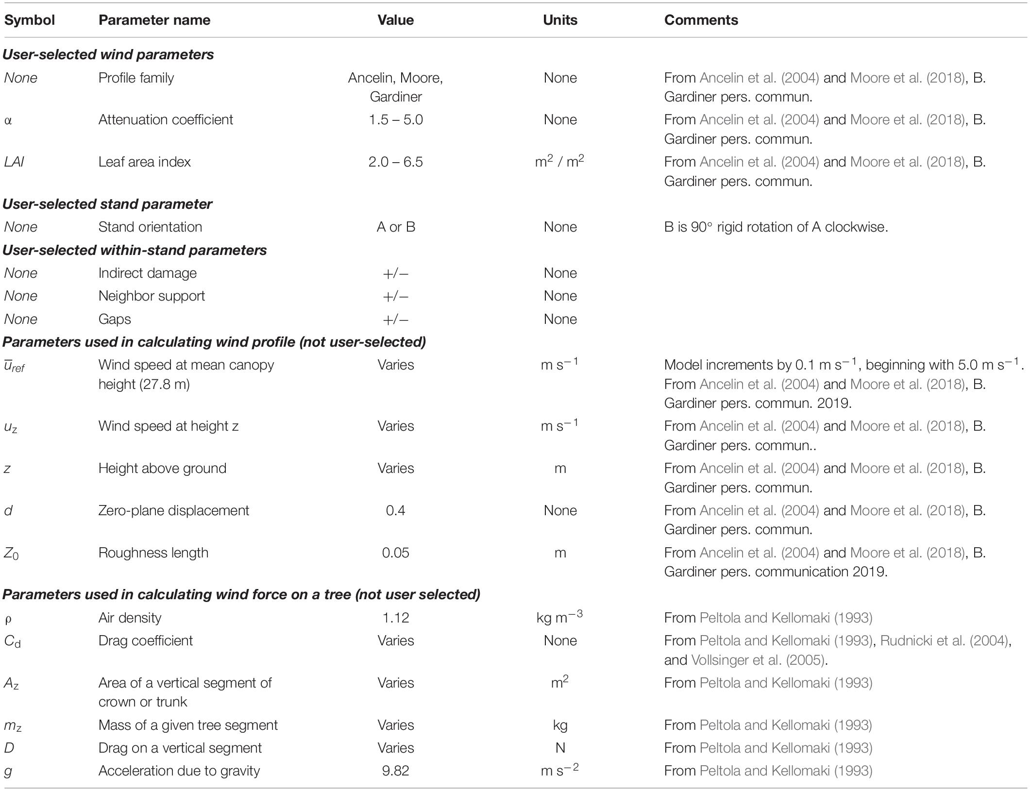
Table 1. Parameters, values and units used in calculation of wind profiles and estimates of CWS.
Drawing on the idea that stands should be considered to fail progressively – with catastrophic mass failure a special case – a dynamic approach changes stand and wind characteristics after each tree failure. The model begins with initial values for canopy height, gustfactor, α, LAI (leaf area index), number of trees, and cumulative horizontal crown area of all trees; all simulations begin with the same values of these parameters. At initiation of each simulation the user chooses one of four possible values for α or LAI; the user chooses the initial α value if Profile Ancelin or Profile Moore are used, or the initial LAI value if Profile Gardiner is used. Initial values of α and LAI are linked such that once the user chooses a value for α, LAI is automatically set to the corresponding value and vice versa. Values of 1.5, 3.0, 4.0, or 5.0 can be chosen for α; the matched values for LAI are 2.0, 3.5, 5.0, and 6.5, respectively. After each tree failure, the program updates the values for canopy height, gustfactor, number of trees, cumulative crown area, α, and LAI, based on the loss of one individual, and the exact horizontal crown area of the fallen tree. After each failure, new canopy height is calculated as the mean of the tallest 50% of remaining trees; this avoids undue influence of understory trees on the canopy height used in the model. The horizontal crown area of each tree is considered a circle with radius equal to the estimated crown radius described above. The updates to α and LAI are based on the cumulative crown area after each failure as a proportion of the original cumulative crown area. Because of this progressive decrease in LAI and α as trees fail, we use the term “beginning attenuation coefficient” or “beginning LAI,” since the specified values are strictly true only for the first tree to fail, and then the values decrease to zero as the number of standing trees approaches zero.
Because one goal of this effort was to examine the influence of relationships based on spatial proximity (e.g., gaps, neighbor support and indirect damage), it was necessary to assemble the trees into a hypothetical virtual stand. Although the winched trees were growing in the same general area (e.g., an area of perhaps 10 ha), their x, y coordinates were not recorded in situ. To make the locations in the virtual stand as realistic as possible, we used the known x, y coordinates from a small section of a large, mapped permanent plot in the same forest type (Hale and Peterson, in preperation). Because our goal was to explore aspects related to spatial complexity and neighbor support, we chose to use real coordinates rather than simulated ones to capture realistic elements such as density gradients and/or spatial clustering. The mapped plot was a mature secondary mixed pine-hardwood forest on the Georgia Piedmont (33.6990° N, −83.2891° W), as was the forest where the winching was conducted (33.1063° N, −83.6756° W). We selected x, y coordinates from trees in the mapped plot that were >15 cm diameter at breast height (dbh), as this was the minimum size of the winched trees. We randomly assigned the winched trees to the coordinates from the mapped plot to create Stand orientation A. Stand orientation B retained the same locations of trees relative to one another, except the locations were a rigid 90° rotation to the right. Both stand orientations were arranged in a square area 54.8 m on each side. This rotation was chosen to mimic winds coming from a different direction (south instead of west). To allow calculation of upwind gaps, and to provide downwind neighbors as potential sources of support, buffer stands were created on both sides of the focal stand. The focal stand was replicated twice on the left side and once on the right, for a total stand of 219.2 m on the x axis (simulating east-west positions), by 54.8 m on the y axis (simulating north-south positions). These replicates, or buffer stands, had the same spatial arrangement as the focal stand. The wind was always assumed to come from the left (west).
Wind velocities are typically reported from meteorological stations as means for some modest interval such as 1 or 3 min (or more); the reported means of course obscure peak wind speeds that result from turbulence and are major determinants of tree failure. The peaks may be several-fold greater than the mean, depending on tree size and spacing. Gardiner et al. (1997) empirically measured turning moment on realistic model trees in a wind tunnel at various spacings and tree heights, and developed a gust factor that converts the drag on a tree at mean wind speed, to the drag at a peak (gust) wind speed. The gust factor was valid for spacings (s, in m) and heights (h, in m) where 0.075 < s/h < 0.45, and is given as:
Where x = distance from forest edge (m). Gustfactor changed for the entire stand as trees progressively failed at higher wind speeds; it was recalculated after every tree failure based on the decrease on total crown area of all trees in the stand. In contrast to the gapfactor (below), gustfactor was the same for all trees in the stand at any given time.
Because the goal of this modelling effort to was to explore the dynamics of tree failure in a progressive fashion until all trees failed, it was necessary to extend the use of gustfactor to tree spacings (densities) beyond the spacing limit of s/h = 0.45 described above. For trees in this study, the value of gustfactor was 4.016 at the of s/h = 0.45. Open terrain with low vegetation would have a gustfactor of 2.1 (B. Gardiner, personal communication); we therefore set the minimum gustfactor at 2.5 when all trees had failed. In the model, once gustfactor reached 4.016, any subsequent tree failures decreased gustfactor linearly from 4.016 to 2.5.
Peltola et al. (1999); see also Seidl et al. (2014) point out that wind forces on trees increase as the size of upwind gaps increase, and that the wind force plateaus at gaps sizes greater than ten tree heights. Seidl et al. (2014) observed that gapfactor varied fivefold from forest interior to the edge of a gap of 10 tree heights; therefore rather than using the formulation given in Peltola et al. (1999), we used a simpler approach of calculating gap size in terms of tree heights, then assigning a value from 1.0 to 5.0 to gapfactor based on current gap size/10.0 (i.e., gap sizes of zero have gapfactor = 1.0, and gaps greater than 10 tree heights in size have gapfactor = 5.0). Gap size was calculated for every tree at every wind speed, and changed as more trees fell and opened larger gaps; we classify it as a within-stand variable.
Gap area was calculated for each tree in each wind speed increment. In our simulations, wind comes only from the left (west), so the area upwind from a focal tree is defined on the x-axis from the center of the focal tree all the way to the left edge of the leftmost portion of the domain. The upwind area is defined on the y axis by the low and high y-axis values of the edges of the focal tree’s horizontal crown. For each focal tree, starting at the lower y axis edge of the crown and repeating every 0.5 m toward the higher y axis edge, we measured the x axis distance from the center of the focal tree to the center of an upwind tree. Thus a focal tree with horizontal crown spread of 3.6 m would result in 8 gap distance measurements. Gap area was defined as the mean of the distances, divided by mean canopy height.
When large trees fail, smaller trees downwind may be in danger of destruction in two distinct ways, which are implemented separately in this model. Indirect damage may occur if there is a substantial size difference and the falling tree is larger; in this case, the smaller downwind tree will be destroyed by being crushed (sensu lato). In the model, a “crush zone” (Figure 2) is defined based on the y-axis dimensions of the falling tree crown, and the total height and crown bottom of the falling tree, which after falling become lower and higher x-axis values. Because the outer edges of falling trees, even when those trees are very large, will typically bend and slide past the smaller downwind trees, the crush zone is only 90% as wide as the y-axis dimensions of the falling tree. This type of interaction occurred if the neighbor was in the crush zone and was less than 50% of the size (defined by dbh) of the falling tree.
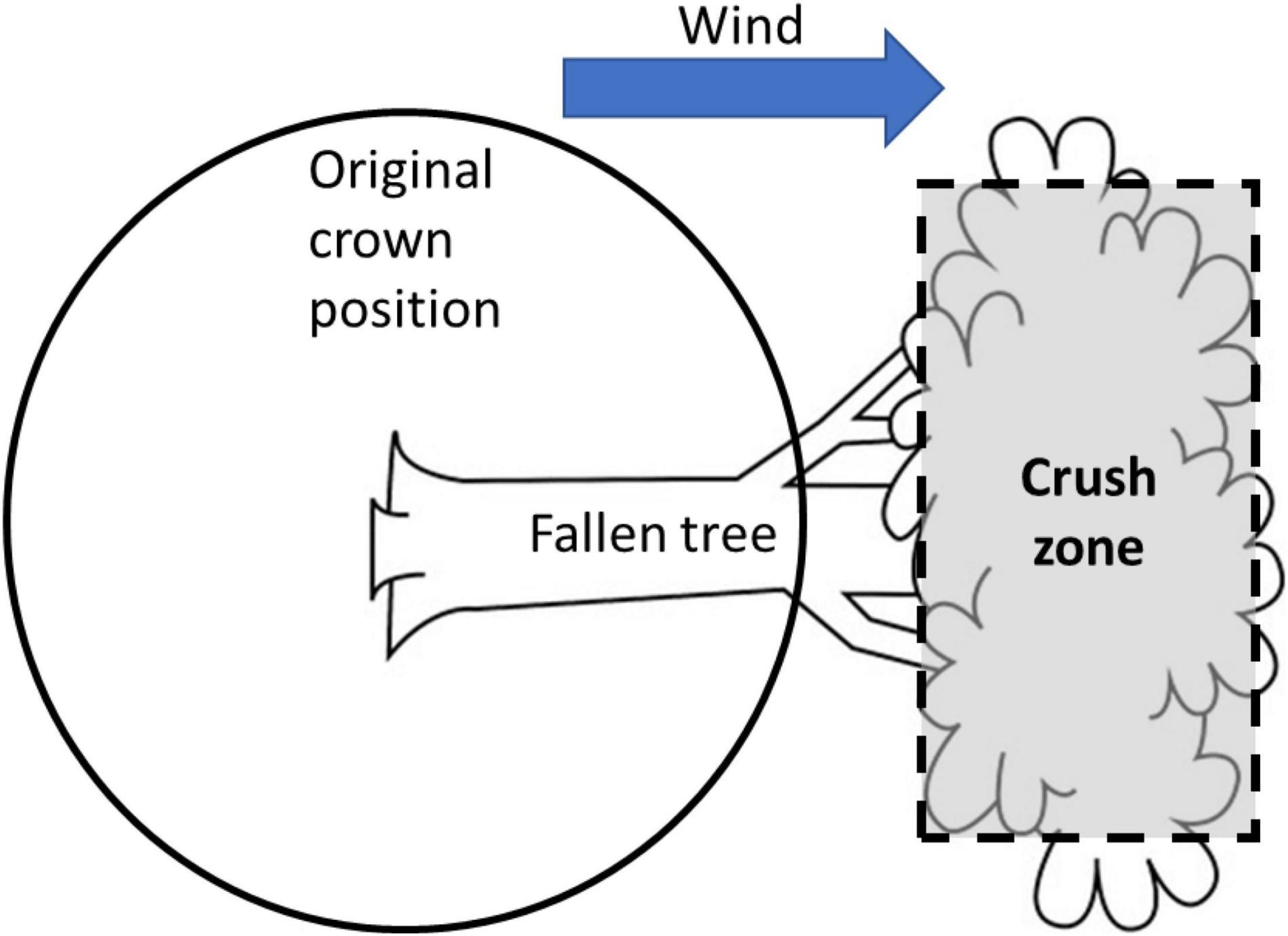
Figure 2. Schematic illustration of the estimation of indirect damage caused by a large tree falling on a smaller neighbor. Crush zone is slightly smaller in the y dimension to allow for bending of outer branch tips of the falling tree.
The most complex focal-neighbor interaction was that of leaning and neighbor support. We emphasize that the implementation in this model is not considered definitive but offered as a reasonable approach to a phenomenon that is well known but whose biomechanics are poorly understood. When a focal tree is pushed by wind from the left, it will lean to the right. Note that currently the model does not include swaying in the sense of repeat bending in roughly opposing directions.
The magnitude of lean is determined by the force of wind on the focal tree; it begins in the model with calculation of the magnitude of lean expected on the basis of the applied force. The leaning angle (from vertical) is calculated from the empirical measured critical angle from the winching study (the angle at which failure occurred) and the empirical measured force on the tree (the force at which failure occurred). For a given wind speed, a proportion is defined as the applied force divided by the measured critical force; this proportion is then used to multiply the measured critical angle to obtain the leaning angle (Figure 3). If no downwind neighbors are nearby, the focal tree deflects to the leaning angle, and no force is offloaded. However, if the focal crown clashes with a downwind neighbor crown prior to reaching the leaning angle, the focal tree temporarily stops deflection at the “stop angle” determined by the distance between the focal and neighbor trees. Figure 3 illustrates some of the process just described; the lateral displacement illustrated determines the stop angle. Focal tree crowns and neighbor tree crowns engage up to the point at which the outer edge of one crown reaches the center point of the other crown; in Figure 3, this is shown as the outer edge of the larger neighbor crown reaching the center point of the focal tree.
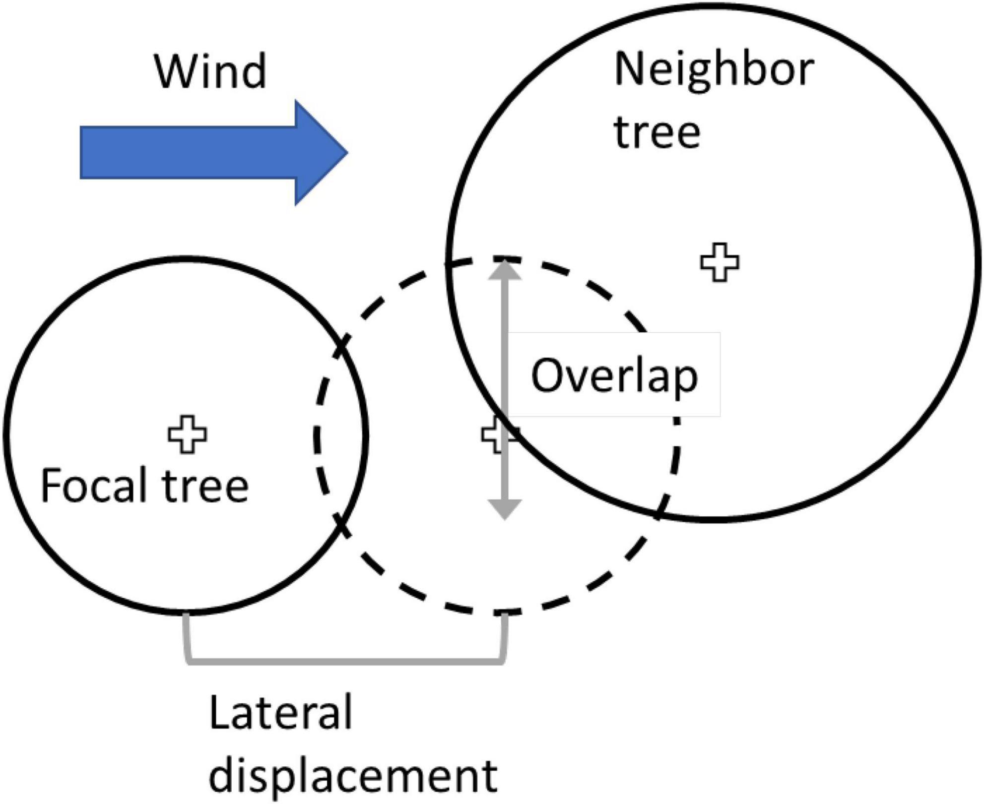
Figure 3. Schematic illustration of the estimation of neighbor support. Smaller solid circle depicts original position of the focal tree, and dotted circle depicts lateral displacement of crown due to wind. Vertical grey arrow illustrates the amount of crown overlap between focal three and neighbor tree.
Following the temporary stop, the focal tree and neighbor tree bend together in very small increments until the combined force needed to bend them any further exceeds the force on the focal tree. Alternatively, if there is enough force on the focal tree to push the neighbor past its own empirically measured critical angle, the neighbor will fail by being pushed over; this is the second form of indirect damage and in our view is distinct from being crushed. As the focal tree and neighbor tree bend together, any force beyond what is needed to bend the focal tree is transferred to the neighbor and causes the neighbor to bend – this is the force offloaded to the neighbor. The small iterations of increasing bending continue as long as the force on the focal tree exceeds the forces necessary to bend the focal and neighbor trees further.
Note that often the crowns of the two trees are sufficiently far apart that the focal tree must lean some amount prior to fully engaging with the neighbor; but in some cases, very near neighbors may have crowns fully engaged prior to any leaning, in which case the stop angle is zero, and the iteration begins with leaning both trees at the lowest wind speed. The amount of force required to lean each tree further will differ because of difference in tree sizes and species, as well as the difference in amount of leaning if the two trees were not fully engaged at zero wind speed. Focal and neighbor trees must have a y-axis overlap of at least 0.5 of the focal crown width for the leaning and transfer to occur.
The offloading of force from focal tree to neighbor has the potential to support the focal tree because the force of wind on the focal tree is spread between both the focal tree and the neighbor, thus potentially increasing the critical wind speed for the focal tree above what it would have been without support. If the focal tree is much larger than the neighbor, then sufficient force may be offloaded to push the neighbor over without providing much support for the focal tree; conversely if the neighbor is much larger, it may function as a very strong supporter, where the focal tree experiences much reduced turning moment.
This approach makes two assumptions that are likely to strongly influence outcomes: First, it assumes that trees bend asynchronously, so whenever a focal tree is bending, the neighbor at that instant is unbent. Second, it assumes that for the calculations being described, only the focal tree experiences the direct force of the wind.
Testing for significant effects of alternative parameter values was conducted as follows. Each run of the model for a particular parameter combination produced a set of 69 critical wind speeds (CWS), for the 69 focal trees in the virtual stand. Given that there were 192 parameter combinations, the combined output was 13,248 critical wind speeds for individual trees. This mass of output was condensed by using the median CWS for each parameter combination in testing, thus yielding tests with n = 192. The condensing is justifiable because performing tests with n = 13,248 would make the tests unduly sensitive, and minute differences between groups (e.g., profile Ancelin vs. profile Moore) may result in tests that were statistically highly significant but not meaningful from a management or science perspective. The six parameters of interest were partitioned into two “wind parameters” (profile families and attenuation factors), one “stand parameter” (tree spatial distribution), and three “within-stand parameters” (direct/indirect damage, support/no support, and gap/no gap). A two-way ANOVA was performed to test for main effects of profile family and attenuation coefficients, and their interactions. The attenuation factors for Profiles Ancelin and Moore was the alpha coefficient, and for Profile Gardiner was the leaf area index (LAI). A t-test was performed to test for effects of stand orientation. And a three-way ANOVA was performed to test for main effects and interactions among the within-stand parameters. These three ANOVAs were utilized because of the near impossibility of interpreting a single six-factor ANOVA and its myriad interactions. Pairwise post hoc tests used the Holm-Sidak method.
To estimate potential effects of silvicultural treatments on the resulting stand wind resistance, three different types of thinning were simulated and compared to unthinned (original) forest. Treatment #1 was a removal of 30% of basal area, culling the smallest trees; treatment #2 was a removal of 60% of basal area, again culling the smallest trees; and treatment #3 was a removal of all hardwoods. Expecting the effects to be consistent across profiles and coefficients, we used a single parameter combination: profile = Ancelin, α = 3.0, stand orientation A, and set the three within-stand parameters to +indirect, +support, and +gaps. We tested for differences in CWS between unthinned forest and three silvicultural treatments, using a one-way ANOVA on ranks, with individual trees as the data points.
The majority of the results presented here report mean CWS, based on a time-averaged wind speed that is multiplied by an empirically derived gust factor. Perhaps surprisingly, the only weather records that we have been able to access in close proximity to our study site report daily maximum wind gust speeds rather than 1 or 3 min mean wind speeds. Therefore we include one figure comparing the time-averaged and instantaneous wind speeds; the latter were estimated by removing the gust factor from the model and outputting the wind speeds that cause failure in the absence of gusts.
The first ANOVA tested for main effects and interactions among three profile families (Ancelin, Moore, and Gardiner), and four attenuation factors. Main effects of profile were highly significant (2 degrees of freedom, F = 54.71, p < 0.001). Pairwise comparisons showed that all pairs were significantly different; median CWS were consistently greatest for the Ancelin profile and least for the Gardiner profile.
Main effects of attenuation factor were also highly significant (3 degrees of freedom, F = 85.65, p < 0.001), and again pairwise comparisons indicated that all pairs were significantly different. The interaction of profile and attenuation factor was highly significant (6 degrees of freedom, F = 3.53, p = 0.003). For all three profile families, greater attenuation factors (α or LAI) cause roughly linear increase in CWS. Because of significant main effects and interactions, all twelve combinations of profile and attenuation factor are shown in Figure 4, with other parameters pooled.
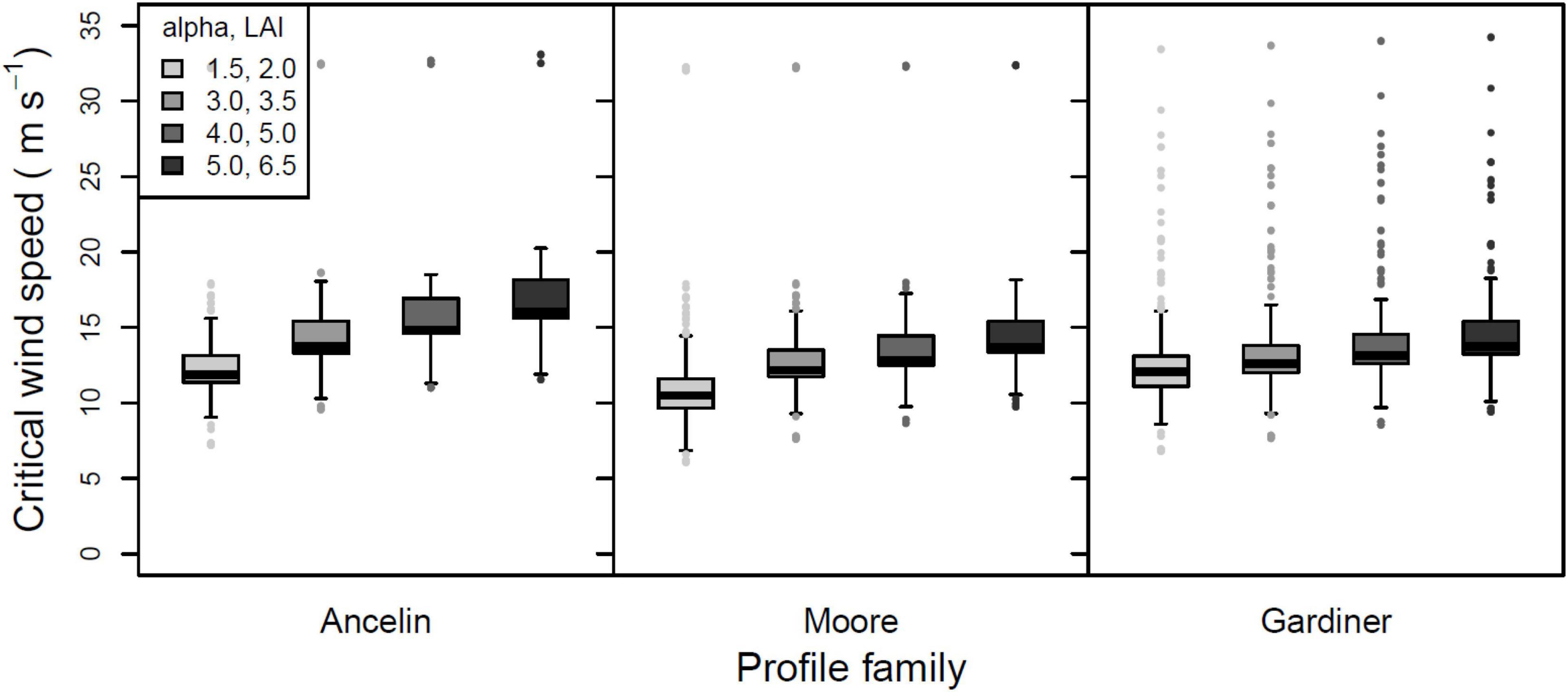
Figure 4. Mean, 25 and 75% percentiles, 1.5× interquartile range (whiskers), and outliers of critical wind speed (CWS) in m s–1, for three profile families and four attenuation factors. For the Ancelin and Moore profile families, the attenuation factor is alpha, with values of 1.5, 3.0, 4.0, and 5.0. For the Gardiner profile family, the attenuation is based on leaf area index (LAI), with values of 2.0, 3.5, 5.0, and 6.5. All other parameters pooled.
The second test compared median CWS from the two alternative stand orientations; this t-test found no difference in CWS between the stand orientations (190 degrees of freedom, t = 0.041, p = 0.967).
The third test was a three-way ANOVA on the three within-stand parameters. Main effects of direct vs. indirect damage were not significant (Figure 5; 1 degree of freedom, F = 0.357, p = 0.551). In contrast, the main effects of support vs. no support (from neighbors) were highly significant (Figure 6; 1 degree of freedom, F = 70.75, p < 0.001), with inclusion of neighbor support leading to a roughly 2 m s–1 increase in median CWS. And main effects of gap vs. no gap were marginally significant (Figure 7; 1 degree of freedom, F = 3.41, p = 0.066); the inclusion of gaps led to a roughly 0.5 m s–1 decrease in median CWS. None of the two-way interactions or the three-way interaction were significant (all had 1 degree of freedom, all F < 0.12, all p > 0.70).
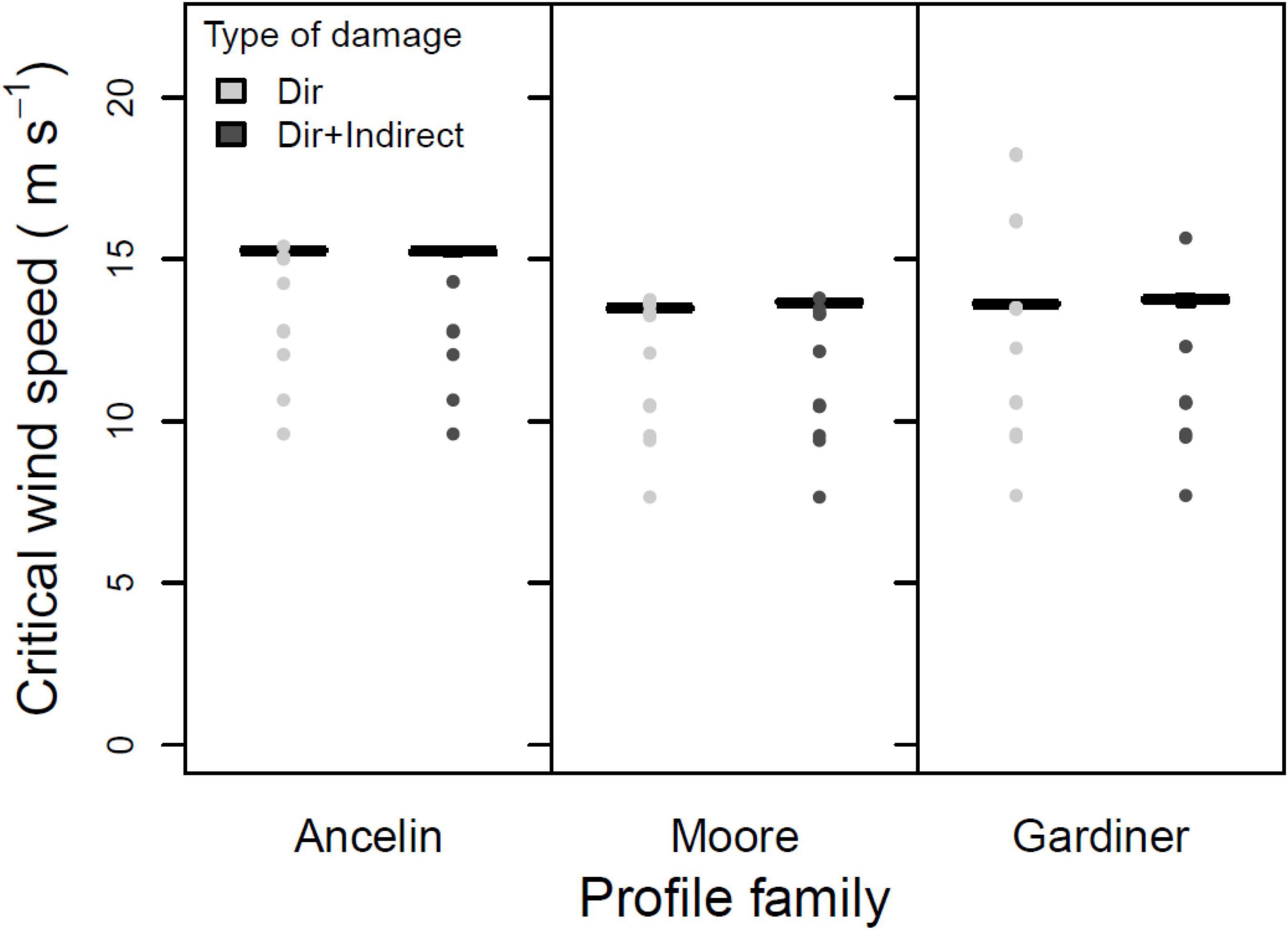
Figure 5. Mean, 25 and 75% percentiles, 1.5× interquartile range (whiskers), and outliers of critical wind speed (CWS) in m s–1, for three profile families, with and without indirect damage. Parameters constant across figure: stand orientation = A; alpha = 3.0 or LAI = 3.5; + neighbor support; + gaps.
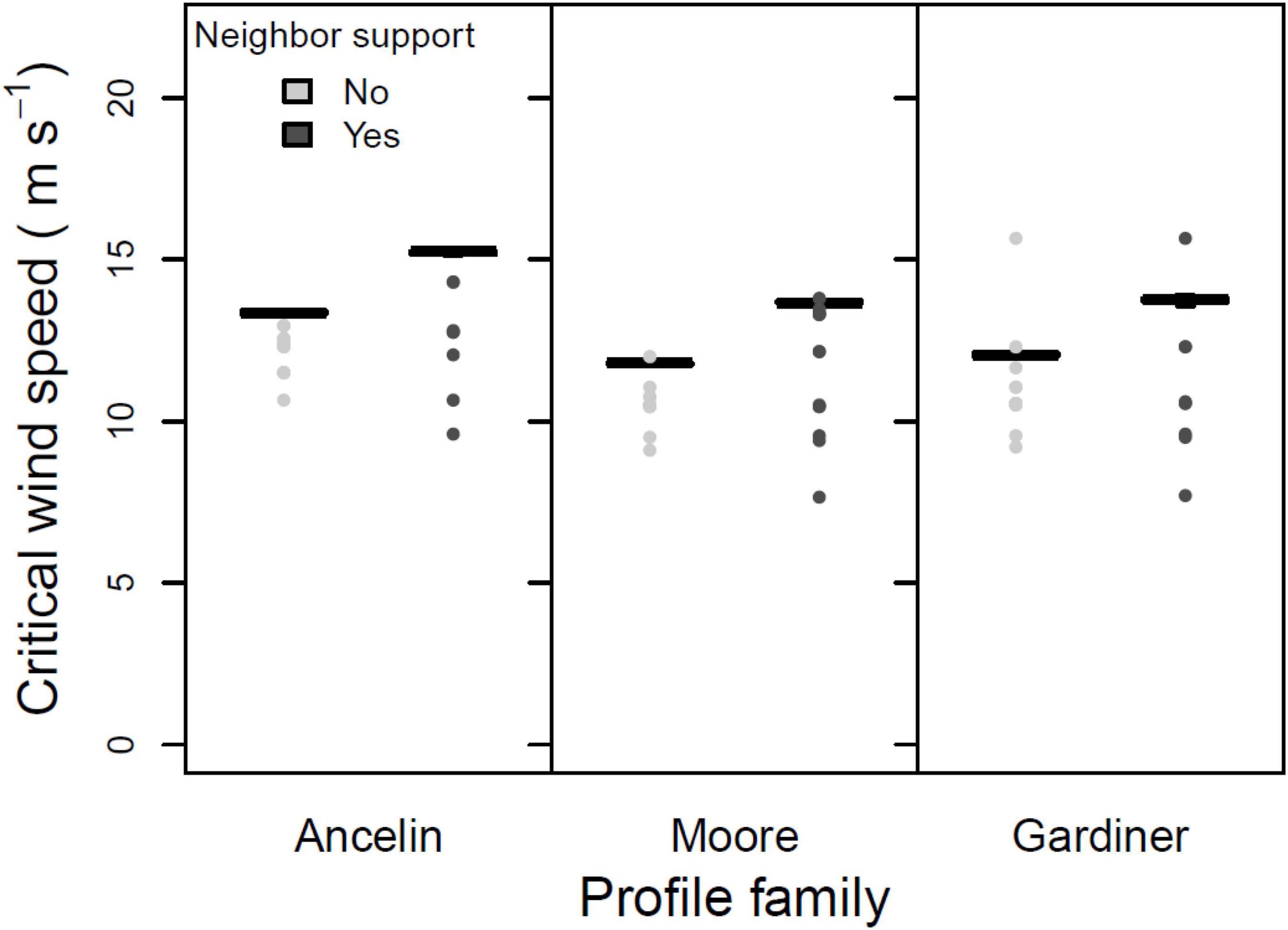
Figure 6. Mean, 25 and 75% percentiles, 1.5× interquartile range (whiskers), and outliers of critical wind speed (CWS) in m s–1, for three profile families, with and without neighbor support. Parameters constant across figure: stand orientation = A; alpha = 3.0 or LAI = 3.5; + indirect damage; + gaps.
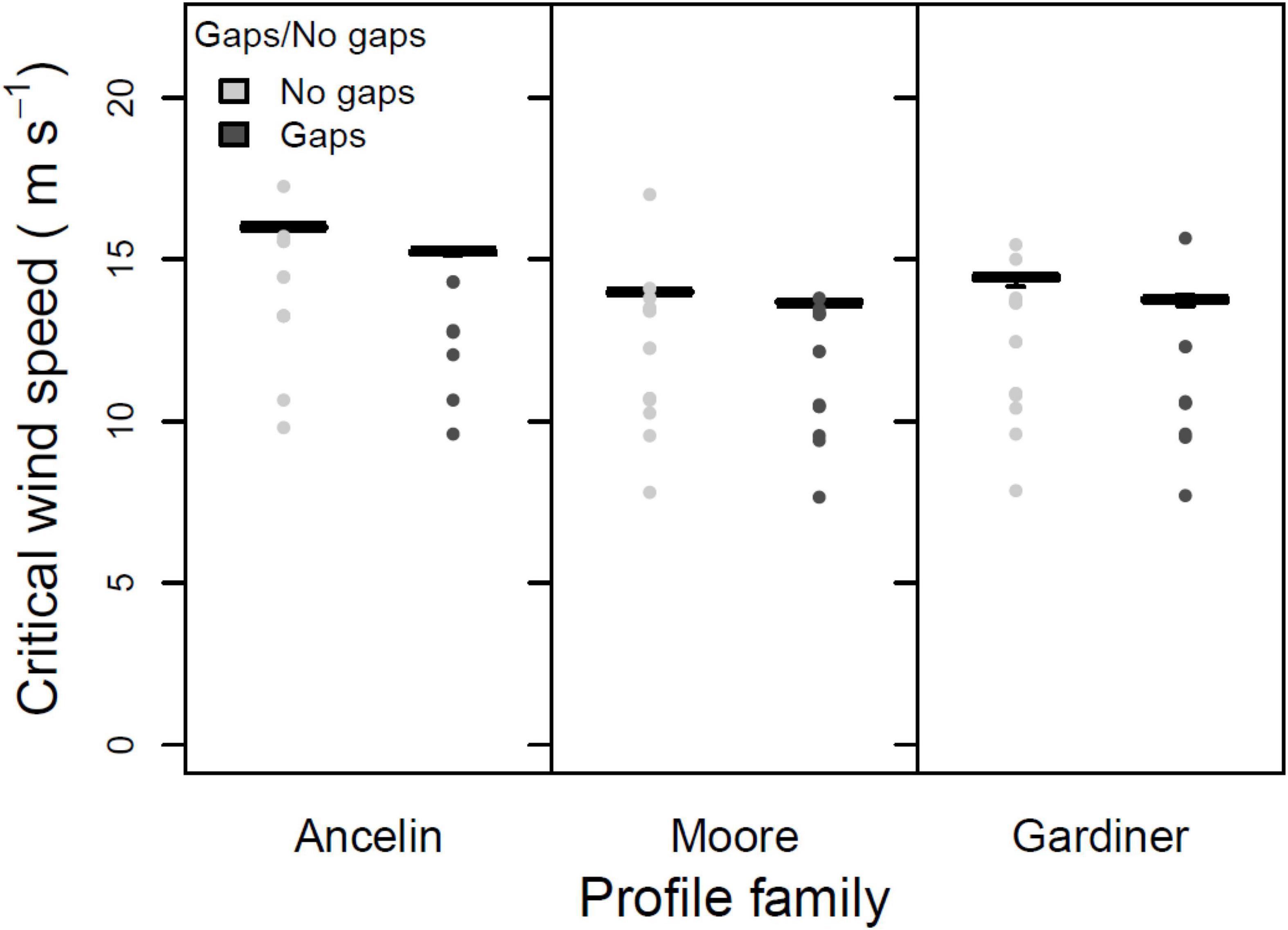
Figure 7. Mean, 25 and 75% percentiles, 1.5× interquartile range (whiskers), and outliers of critical wind speed (CWS) in m s–1, for three profile families, with and without gaps. Parameters constant across figure: stand orientation = A; alpha = 3.0 or LAI = 3.5; + indirect damage; + neighbor support.
Silvicultural treatments led to significant differences in CWS when compared to unthinned forest (Figure 8). Overall, differences among the control and three treatments were highly significant (Kruskal-Wallis test, 3 degrees of freedom, H = 101.18, p < 0.001). Pairwise comparisons showed that all three silvicultural treatments had significantly higher CWS than the unthinned control (Dunn’s tests, p < 0.05); among the thinned treatments, CWS were lowest in the hardwood removal, and highest in the 60% thinning treatment.
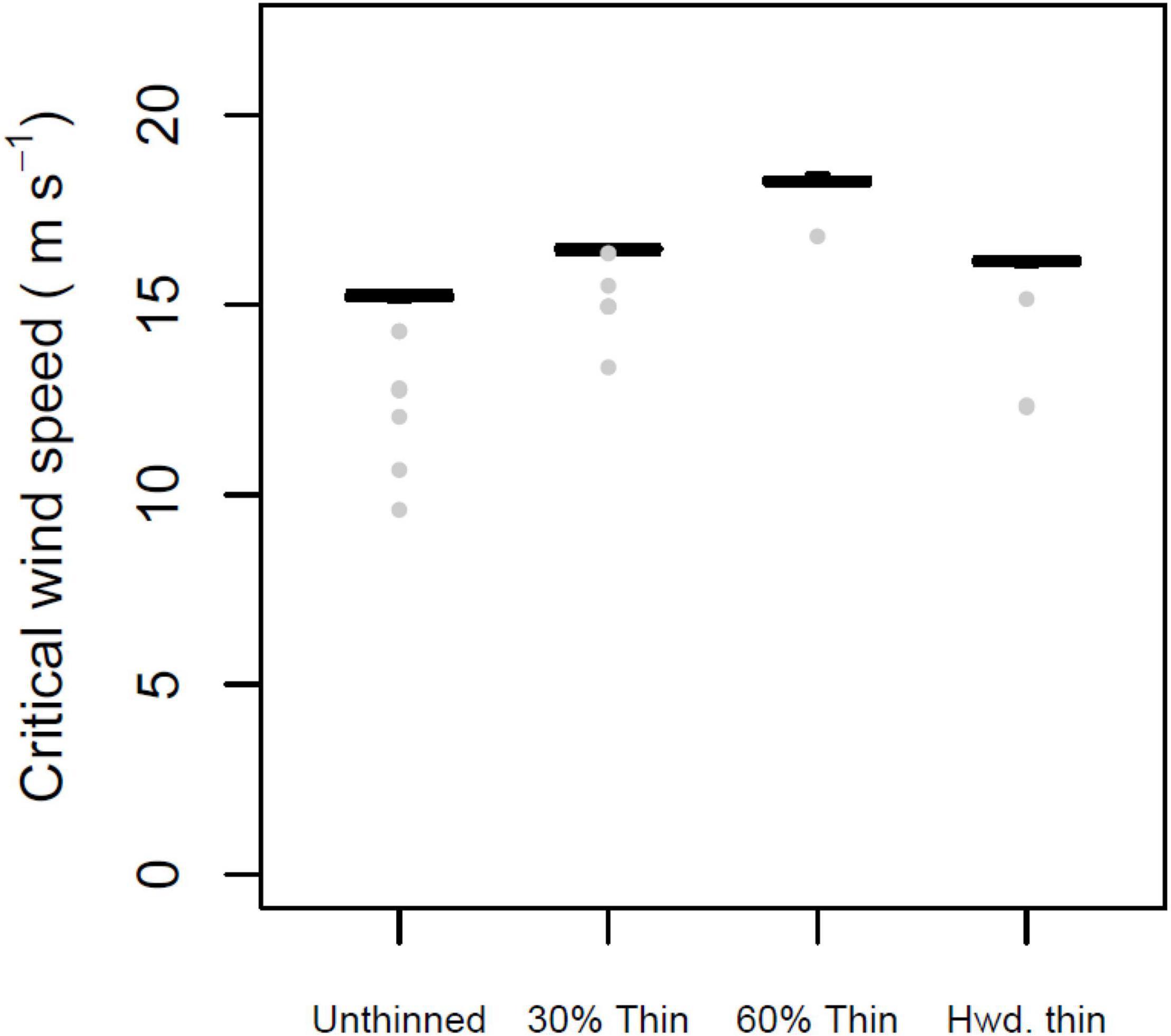
Figure 8. Mean, 25 and 75% percentiles, 1.5× interquartile range (whiskers), and outliers of critical wind speed (CWS) in m s–1, for intact forest and three silvicultural treatments. A 30% thin removed smallest trees up to 30% of basal area. A 60% thin removed smallest trees up to 605 of basal area. Parameters constant across figure: Profile family = Ancelin; stand orientation = A; alpha = 3.0 or LAI = 3.5; + indirect damage; + neighbor support.
The instantaneous wind speeds that cause tree failure are roughly threefold greater than the mean wind speeds (Figure 9). For the four parameter combinations used for this illustration the medians of each set of 69 CWS, were 11.9, 13.65, 13.35, and 15.25 m s–1 for mean CWS, and 32.4, 38.15, 42.9, and 36.6 m s–1 for instantaneous CWS.
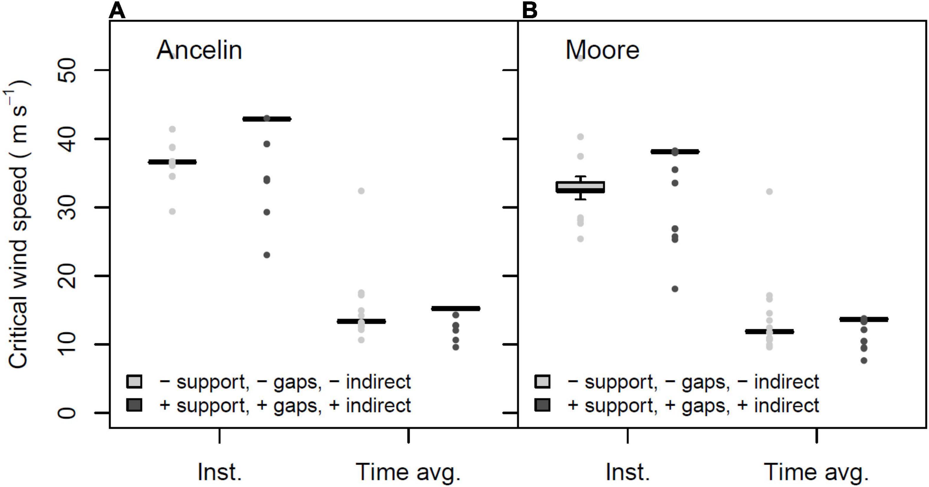
Figure 9. Mean, 25% and 75% percentiles, 1.5× interquartile range (whiskers), and outliers of critical wind speed (CWS) in m s–1, for intact forest under two profile families, presented as time-averaged mean wind speeds and instantaneous wind speeds. (A) Profile family Ancelin; (B) profile family Moore. Parameters constant across figure: stand orientation = A; alpha = 3.0 or LAI = 3.5.
This work represents the first attempt that we know of, to model critical wind speeds and wind damage dynamics for southeastern U.S. Piedmont forests. These forests are largely minimally managed, mature pine-hardwood mixtures, with multiple cohorts and moderate to high species richness. The model presented here, called ForSTORM, yields results consistent with some of our expectations, but also produces unexpected insights. We emphasize that because this is based on a single winching study and is a first version of the model, further winching studies and refinements of the model are desirable to reach more robust conclusions.
Our aim was to explore the effects of several wind and stand characteristics that have been the subject of much less study than typical tree characteristics such as height or slenderness. To facilitate such investigation, we utilized three wind profile families, four attenuation coefficients, two different stand orientations, presence or absence of gaps, presence or absence of neighbor support, and direct only or direct + indirect damage. One unique aspect of this model is that indirect damage may occur in one of two ways: either by a leaning tree pushing over a neighbor, or by a large tree crushing a substantially smaller neighbor after the large tree has begun to fall.
The wind profile families were based on Ancelin et al. (2004) and Moore et al. (2018), and a personal communication from B. Gardiner; even when provided with similar attenuation coefficients or leaf area index values (LAI), the resulting profiles were visibly distinct (Figure 1), and differences were greater for low attenuation (alpha = 1.5 or LAI = 2.0). The Ancelin profile exhibits a more drastic decrease in wind speed within the canopy: when above-canopy wind speed is 30 m s–1 and alpha = 3.0, the wind speed at 20 m is 7.89 m s–1 in the Ancelin profile and 11.60 m s–1 in the Moore profile. Consequently, even when attenuation coefficients were identical for profiles Ancelin and Moore, trees failed at slightly lower CWS under the Moore profile, and at higher CWS under the Ancelin profile, apparently because somewhat higher winds penetrate deeper into the canopy with the Moore profile. We infer that stand failure dynamics are sensitive to subtle differences in the vertical distribution of wind speeds, and that our prediction #1 was supported. Practically, this implies that tree CWS will be lower when profiles attenuate above-canopy winds to a lesser degree.
As expected, greater beginning attenuation coefficients caused the below-canopy profiles to become progressively more curved, with much slower wind speeds near the ground (Figure 1), although the attenuation steadily diminishes during any given run of the model as more trees fail. Several implications emerge from the damage patterns seen at different attenuation coefficients (Figure 4). First, our prediction #2 was confirmed; in all scenarios, lower attenuation coefficients resulted in lower CWS, a result of greater wind velocities at lesser heights. Second, the differences in CWS produced by increasing attenuation coefficients are greater for the Ancelin profile family than for the other two profile families. This trend is likely to be a major driver of the statistically significant interaction between profile family and attenuation, and it derives from the Ancelin profile producing a very rapid decrease in wind speeds just below the mean canopy height when attenuation coefficient or LAI is high.
It is worth noting that a number of previous studies (Achim et al., 2005; Cucchi et al., 2005; Locatelli et al., 2016; Duperat et al., 2020) report lower CWS when stand densities are lower; it is likely that such a trend is driven in large part by decreased attenuation as a result of lower LAI when density is low, allowing the wind to penetrate more deeply into stands and more easily push trees to failure.
The two alternative stand orientations resulted in minimal differences in the distribution of CWS, thus not supporting our hypothesis #3.. Differences between stand orientations were essentially non-existent for beginning attenuation coefficients of 3.0, and slightly greater for attenuation coefficients of 1.5. In retrospect, this may not be surprising, because the two stand orientations were effectively the same stand with the wind coming from a different direction. Because neither our model nor our input data included any adjustment to tree wind resistance as a function of wind direction, and because the overall spatial distribution of trees is rather uniform (for a natural stand), the variation in wind experienced by different trees in the alternative orientations may be minimal. These findings cannot tell us about potential effects of larger differences in stand spacing, but they do suggest that the CWS dynamics during stand failure are not highly sensitive to subtle differences in spatial arrangement of trees. We are not aware of published research in relation to this question, so it is difficult to place our findings in the context of other work.
Inclusion of indirect damage along with direct damage neither increased nor decreased overall CWS in comparison to direct damage only, thereby providing no support to our hypothesis #4 (Figure 5). This may be because the number of trees that failed by being crushed was modest, varying only between 13 and 17; such limited number of trees may have been insufficient to lead to substantial differences in overall CWS. In most cases, the distribution of failure from crushing was concentrated early in the failure sequence; for example in results from several different parameter combinations, the first nine (out of 13) crushed trees to fail were in the first half of the failure sequence. It is possible that a different method to calculate probability of crushing small neighbors would increase the importance of indirect damage, but to date this form of indirect damage has been modeled only a few times and a consensus approach to indirect damage has yet to emerge. Indirect damage was included in the ForGEM model (Schelhaas et al., 2007), but – consistent with our findings here – it led to only a small proportion of trees being damaged due to falling larger neighbors.
The neighborhood interaction with by far the greatest effect on CWS was the presence or absence of neighbor support (Figure 6). In all scenarios examined, inclusion of neighbor support increased CWS; including neighbor support typically increased mean CWS by roughly 1.5 m s–1 – an increase of about 15%. The increase in CWS as a result of including neighbor support was consistent across the three profile families, and did not depend on presence or absence of gaps or on whether indirect damage was included. Therefore, our results strongly support hypothesis #5.
Neighborhood interactions of sheltering and support are included in the wind damage module of the landscape model iLand, but they are combined in the form of a competition index (Seidl et al., 2014), thus preventing separate consideration of sheltering and support. That said, sheltering and support significantly increased CWS for trees in their simulations. Similarly, neighbor support significantly increased tree stability in the ForGEM model (Schelhaas et al., 2007). These authors note that in high-density stands, tree slenderness increased and would have caused greater vulnerability, but that vulnerability was counterbalanced by the greater support provided by neighbors in the high-density stands.
The presence or absence of gaps led to small but consistent differences in CWS during stand failure (Figure 7), with slightly lower CWS when the model was run with gaps; these differences were marginally significant (p = 0.066 in the ANOVA). Thus model results provided limited support for our prediction #6.
This finding is qualitatively consistent with a variety of studies of effects of surroundings on stability of trees in an isolated stand; most such studies reveal that greater openness (corresponding to larger gaps in our model) result in greater risk and thus lower CWS to the trees in the stand, at least until the trees along the stand edges have acclimated (Zeng et al., 2010; Anyomi and Ruel, 2015; Locatelli et al., 2016; Ruel and Gardiner, 2019). However, the effect of gaps in this study is small, and raises the question of whether an alternative implementation of the gap effect would produce substantially greater gap influence in the tree failure sequence. We chose to limit the effect of upwind gaps to trees directly on the downwind edge of gaps, with no effect on trees that did not directly border the gaps – this implies that wind from gaps does not penetrate the stand, an assumption that could minimize gap effects in the model.
As implemented here, our model results provide some basis to inform silvicultural decisions. All three of the thinning treatments resulted in increased CWS, with the heavier thinning leading to a greater increase in CWS. If such a trend is robust, it implies that thinnings need not increase risk of windthrow and the accompanying financial losses. This at first may be surprising because thinning of course reduces density, which in turn lowers LAI and attenuation, allowing winds to penetrate deeper into the stand. Such changes by themselves should increase wind forces on the trees and thereby reduce CWS. However, it is likely that the thinning removed weaker trees: all three treatments removed smaller trees, which might be expected to have a more slender morphology due to growing in mid- or subcanopy positions (Kozak et al., 1969; Martin, 1981). Indeed, the height:diameter ratio of removed and remaining trees in the 30% thinning treatment was 65.4 and 77.9, respectively, suggesting the removed trees were more vulnerable. Similar trends were observed for the 60% thin and hardwood thin treatments; in both cases, the thinned trees had higher height:diameter ratios, suggesting the remaining trees were more stable than the removed trees. Hypothetically, evaluating the possible consequences of a thinning prescription would thus involve weighing the potential negative effects of increased wind penetration against the potential to remove the most vulnerable trees. While forest managers may not have sufficient information to quantitatively compare these risks and benefits, it is likely that the potential increase in risk will be minimal as long as the main canopy trees remain in place.
The nearest reliable weather recording station to our study site is the U.S.D.A. Forest Service Remote Automated Weather Station for Oconee County (33° 12′ 30″, −83° 42′ 29″), 11.6 km from our study site. This station could provide weather data from 2010 onwards; we chose to analyze 2010–2020 weather. Based upon maximum daily gust speed, the return times for winds of 18–20 m s–1 was once per 10.87 years; for 15 m s–1 it was once per 1.81 years. Referring to Figure 9, the instantaneous wind speeds that are likely to cause substantial damage to our virtual stand are in the range of 30 – 40 m s–1. Because no events of that magnitude were recorded during 2010–2020, we cannot precisely estimate the frequency with which such winds occur, although the obvious conclusion is that such winds likely occur with multi-decade frequency, or perhaps longer. Thus there appears to be a low probability that winds strong enough to damage a large fraction of our virtual stand would be expected within a single rotation period. This is consistent with broader trends in high wind frequency reported for much of the central hardwood forest type in eastern U.S. (Peterson et al., 2016); severely damaging winds are unlikely within a 50–70 yr rotation period but may be expected once or twice within the lifespan of the dominant species.
At a very basic level, our model relies on findings from static winching studies, which have a number of limitations. Most such studies do not mimic tree swaying, and only a few include consideration or manipulation of soil moisture. Drag coefficients are poorly known for most species, and crown dimensions are only roughly approximated. We chose Cd values from Rudnicki et al. (2004) and Vollsinger et al. (2005); however, other values are available. Katul et al. (2004) reported Cd of 0.2 for a loblolly pine stand in North Carolina and a Cd of 0.15 for a mixed pine-hardwood stand in Tennessee. If we use these values as streamlined Cd for pines and hardwoods in our model, and begin with a still air Cd of 0.6 [approximated from Mayhead (1973)], the predicted CWS increase by roughly 35% (parameters used were Ancelin profile, stand orientation A, α = 3.0, and the three within-stand parameters set to “on” or “yes”). It is not clear when accurate drag coefficients will be available for a larger number of southeastern U.S. species, but these findings make clear that the quantitative CWS results are strongly influenced by the drag coefficients.
The narrow vertical dimension of the boxes in Figures 4–9 and the flattened sequences in Figure 10 are a result of rapid progression of tree failure after the first few trees fail, in response to only minute increases in wind speed. While the wind speeds at which this happens in our model are plausible, we suspect that real trees in real forests fail at a wider range of wind speeds. We suspect the cause is one or both of two related phenomena in our model. First, the change in wind field may progress too rapidly, i.e., the failure of a single tree in real forests may not alter the wind field for the remaining trees as rapidly as it does on our simulations. Second, the fundamental approach of adjusting the wind field sequentially after each tree failure may be a poor mimic of natural failure dynamics; an alternative approach would be to adjust the wind field after each increment of wind speed rather than after each tree failure. Future work with this model will explore several alternatives.
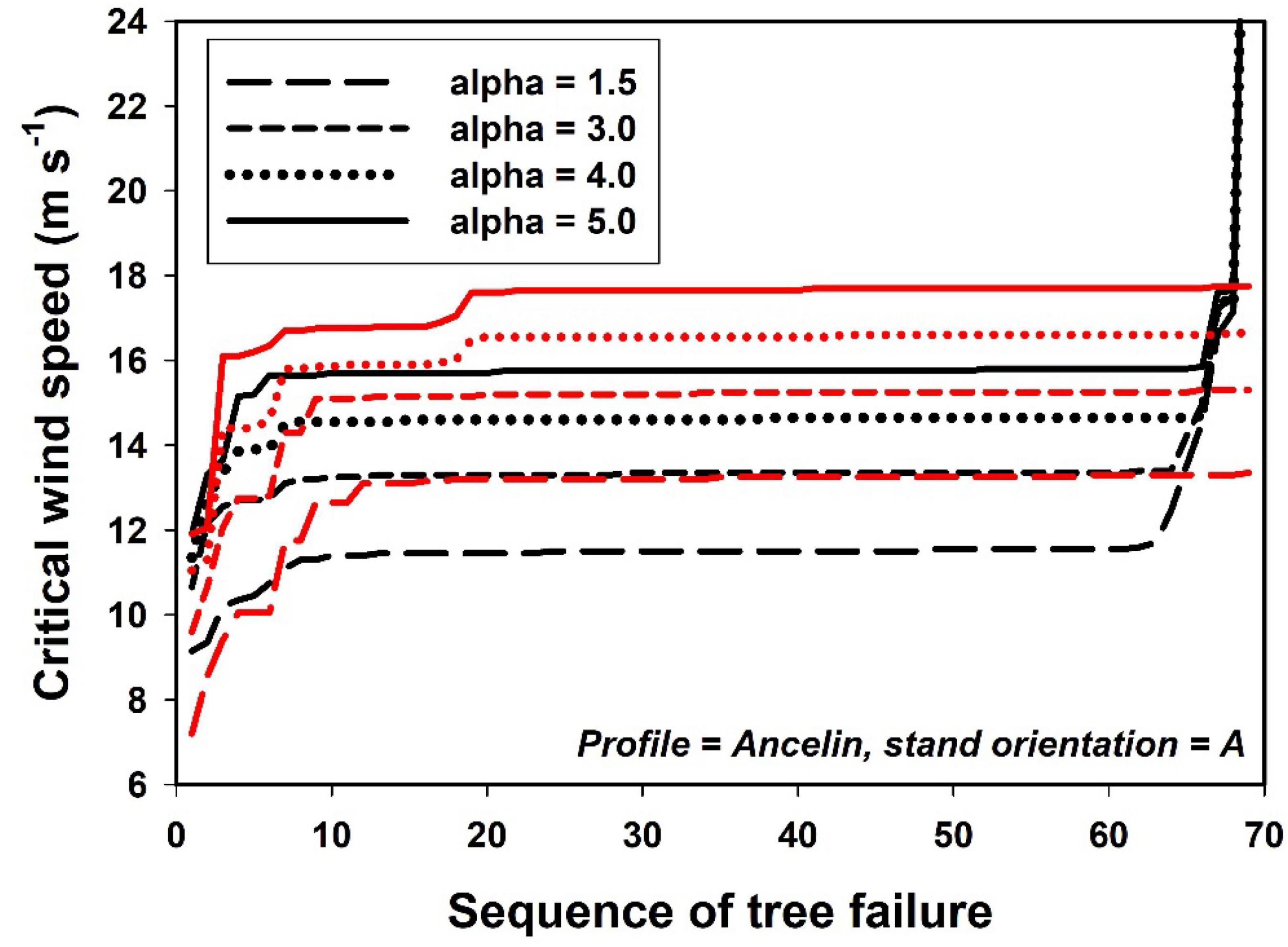
Figure 10. Critical wind speed plotted against sequence of tree failure, for four values of attenuation coefficient (alpha), and contrasting combinations of within-stand parameters. Black lines = – indirect damage; – neighbor support; and – gaps. Red lines = + indirect damage; + neighbor support; + gaps.
This model implements a number of interactions and processes in ways that may differ from the models produced by other authors, and such differences may contribute to differences in findings. That is not to say one implementation is correct and others are wrong, because different authors have different objectives. For example, our model separates indirect damage from neighbor support, whereas the wind damage module of iLand combines these interactions (Seidl et al., 2014). Similarly, gaps are included in this model differently than in ForGEM (Schelhaas et al., 2007). Direct comparison among the protocols for modelling these various interactions may reveal if one formulation has advantages over others.
Another area for potential improvement is that some phenomena are simply not included. Our model assumes independent tree sways. This is a simplification to facilitate computational efficiency, but sway of real trees is at least partially synchronized. A major potential improvement would be to formulate our model with partial synchronization among the trees. Along with the need for improved swaying, our model implicitly assumes spatially and temporally uniform wind fields, as well as no consideration of wind duration and the potential effect of wood fatigue. All of these factors are likely to influence failure dynamics in real trees and forests; future versions of our model will include some of these possible improvements.
The raw data supporting the conclusions of this article will be made available by the authors, without undue reservation.
CP participated in winching, wrote C++ code, ran simulations, and wrote the manuscript. JC participated in the winching, wrote the winching manuscript, and edited manuscript. Both authors contributed to the article and approved the submitted version.
Funding during the 2012 field season was based on National Science Foundation grant DEB-1143511 from Population and Community Ecology, and for some of the early phases, JC was supported by a Climate Change Youth Initiative fellowship from the U.S. National Park Service.
The authors declare that the research was conducted in the absence of any commercial or financial relationships that could be construed as a potential conflict of interest.
All claims expressed in this article are solely those of the authors and do not necessarily represent those of their affiliated organizations, or those of the publisher, the editors and the reviewers. Any product that may be evaluated in this article, or claim that may be made by its manufacturer, is not guaranteed or endorsed by the publisher.
We thank Carl Schmidt and the Piedmont National Wildlife Refuge for making available the land and trees for the winching study. Many field assistants braved often brutal summer heat to complete the winching. This study would not have begun in the absence of our earlier Amazon study, for which we owe thanks to Giga Ribiero, Jeff Chambers, and all of our co-authors. We also thank Barry Gardiner for numerous beneficial discussions and Barry Gardiner and Jean-Claude Ruel for inviting us to contribute to this special issue.
Achim, A., Ruel, J.-C., Gardiner, B. A., Laflamme, G., and Meunier, S. (2005). Modeling the vulnerability of balsam fir forests to wind damage. For. Ecol. Manag. 204, 35–50. doi: 10.1016/j.foreco.2004.07.072
Ambinakudige, S., and Khanal, S. (2010). Assessment of impacts of Hurricane Katrina on net primary productivity in Mississippi. Earth Interact. 14, 1–12. doi: 10.1175/2010EI292.1
Ancelin, P., Courbaud, B., and Fourcaud, T. (2004). Development of an individual tree-based mechanical model to predict wind damage within forest stands. For. Ecol. Manag. 203, 101–121. doi: 10.1016/j.foreco.2004.07.067
Anyomi, K. A., and Ruel, J.-C. (2015). A multiscale analysis of the effects of alternative silvicultural treatments on windthrow within balsam fir dominated stands. Can. J. For. Res. 45, 1739–1747.
Asner, G. P., Scurlock, J. M. O., and Hicke, J. A. (2003). Global synthesis of leaf area index observations: implications for ecological and remote sensing studies. Glob. Ecol. Biogeogr. 12, 191–205. doi: 10.1046/j.1466-822X.2003.0026.x
Blackburn, P., and Petty, J. A. (1988). Theoretical calculations of the influence of spacing on stand stability. Forestry 61, 235–244.
Cannon, J. B., Barrett, M. E., and Peterson, C. J. (2015). The effect of species, size, failure mode, and fire-scarring on tree stability. For. Ecol. Manag. 356, 196–203.
Cassels, L. (2020). Two Years Later, Relief For Timber Losses Due To Hurricane Michael Is Authorized. Miami, FL: Florida Phoenix.
Chambers, J. Q., Fisher, J. I., Zeng, H., Chapman, E. L., Baker, D. B., and Hurtt, G. C. (2007). Hurricane Katrina’s carbon footprint on U.S. Gulf Coast forests. Science 318:1107. doi: 10.1126/science.1148913
Cionco, R. M. (1978). Analysis of canopy index values for various canopy densities. Boundary-Layer Meteorol. 15, 81–93. doi: 10.1007/BF00165507
Cucchi, V., Meredieu, C., Stokes, A., Coligny, F., Suarez, J., and Gardiner, B. A. (2005). Modelling the windthrow risk for simulated forest stands of Maritime pine (Pinus pinaster Ait.). For. Ecol. Manag. 213, 184–196.
Duperat, M., Gardiner, B., and Ruel, J.-C. (2020). Testing an individual tree wind damage risk model in a naturally regenerated balsam fir stand: potential impact of thinning on the level of risk. Forestry 94, 141–150. doi: 10.1093/forestry/cpaa023
Elie, J.-G., and Ruel, J.-C. (2005). Windthrow hazard modelling in boreal forests of black spruce and jack pine. Can. J. For. Res. 35, 2655–2663.
Gardiner, B., Byrne, K., Hale, S., Kamimura, K., Mitchell, S. J., Peltola, H., et al. (2008). A review of mechanistic modelling of wind damage risk to forests. Forestry 81, 447–463. doi: 10.3732/ajb.93.10.1501
Gardiner, B., Peltola, H., and Kellomaki, S. (2000). Comparison of two models for predicting the critical wind speeds required to damage coniferous trees. Ecol. Modell. 129, 1–23. doi: 10.1016/S0304-3800(00)00220-9
Gardiner, B. A., Stacy, G. R., Belcher, R. E., and Wood, C. J. (1997). Field and wind tunnel assessments of the implications of respacing and thinning for tree stability. Forestry 70, 233–252.
Gordon, J. S., Auel, J. B., Blair-Agyeman, N. I, Montague, B., and Shmulsky, R. (2018). Infrastructure enhancement to support value-added bioproduct recovery. Natural Resour. 09, 129–149.
Hart, E., Sim, K., Kamimura, K., Meredieu, C., Guyon, D., and Gardiner, B. (2019). Use of machine learning techniques to model wind damage to forests. Agric. For. Meteorol. 265, 16–29. doi: 10.1016/j.agrformet.2018.10.022
Hedden, R. L., Fredericksen, T. S., and Williams, S. A. (1995). Modeling the effect of crown shedding and streamlining on the survival of loblolly pine exposed to acute wind. Can. J. For. Res. 25, 704–712.
Holzmueller, E. J., Gibson, D. J., and Sucheki, P. F. (2012). Accelerated succession following an intense wind storm in an oak-dominated forest. For. Ecol. Manag. 279, 141–146.
Jackson, T. (2019). Hurricane Michael Recovery Focus of State Line Meeting. Compass Live. Asheville, NC: USDA Forest Service Southern Research Station.
Katul, G. G., Mahrt, L., Poggi, D., and Sanz, C. (2004). One- and two-equation models for canopy turbulence. Boundary Layer Meteorol. 113, 81–109.
Kozak, A., Munro, D. D., and Smith, J. H. G. (1969). Taper functions and their application in forest inventory. For. Chron. 45, 278–283.
Krejci, L., Kilejka, J., Vozenilek, V., and Machar, I. (2018). Application of GIS to empirical windthrow risk model in mountain forested landscapes. Forests 9:96. doi: 10.3390/f9020096
Landsberg, J. J., and James, G. B. (1971). Wind profiles in plant canopies: studies on an analytical model. J. Appl. Ecol. 8, 729–741.
Locatelli, T., Gardiner, B., Tarantola, S., Nicoll, B., Bonnefond, J. M., Garrigou, D., et al. (2016). Modelling wind risk to Eucalyptus globulus (Labill.) stands. For. Ecol. Manag. 365, 159–173. doi: 10.1016/j.foreco.2015.12.035
Martin, A. J. (1981). Taper and Volume Equations for Selected Appalachian Hardwood Species. USDA Forest Service, Research Paper NE-490. Broomall, PA: U.S. Dept. of Agriculture, Forest Service, 26.
Mayhead, G. J. (1973). Some drag coefficients for British forest trees derived from wind tunnel studies. Agric. Meteorol. 12, 123–130.
Moore, J., Gardiner, B., and Sellier, D. (2018). “Tree mechanics and wind loading,” in Plant Biomechanics, eds A. Geitmann and J. Gril (Berlin: Springer), 79–106.
Peltola, H., and Kellomaki, S. (1993). A mechanistic model for calculating windthrow and stem breakage at stand edge. Silva Fenn. 27, 99–111.
Peltola, H., Kellomaki, S., Vaisanen, H., and Ikonen, V.-P. (1999). A mechanistic model for assessing the risk of wind and snow damage to single trees and stands of Scots pine, Norway spruce, and birch. Can. J. For. Res. 29, 647–661. doi: 10.1139/cjfr-29-6-647
Peterson, C. J. (2007). Consistent influence of tree diameter and species on damage in nine eastern North America tornado blowdowns. For. Ecol. Manag. 250, 96–108.
Peterson, C. J., Cannon, J. B., and Godfrey, C. M. (2016). “First steps toward defining the wind disturbance regime in Central Hardwoods forests,” in Natural Disturbance and Historic Range of Variation, eds C. H. Greenberg and B. S. Collins (Berlin: Springer), 89–122.
Peterson, C. J., Ribeiro, G. H. P. M., Negron-Juarez, R., Marra, D., Chambers, J. Q., Higuchi, N., et al. (2019). Critical wind speeds suggest wind could be an important disturbance agent in Amazonian forests. Forestry 94, 444–459. doi: 10.1093/forestry/cpz025
Rudnicki, M., Mitchell, S. J., and Novak, M. D. (2004). Wind tunnel measurements of crown streamlining and drag relationships for three conifer species. Can. J. For. Res. 34, 666–676.
Ruel, J.-C., and Gardiner, B. (2019). Mortality patterns after different levels of harvesting of old-growth boreal forests. For. Ecol. Manag. 448, 346–354. doi: 10.1016/j.foreco.2019.06.029
Rutledge, B. T., Cannon, J. B., McIntyre, K., Holland, A. M., and Jack, S. B. (2021). Tree, stand, and landscape factors contributing to hurricane damage in a coastal plain forest: post-hurricane assessment in a longleaf pine landscape. For. Ecol. Manag. 481:118724.
Sampson, D. A., Vose, J. M., and Allen, H. L. (1998). “A conceptual approach to stand management using leaf area index as the integral of site structure, physiological function, and resource supply,” in Proceedings of the 9th Biennial Southern Silviculture Conference. USDA Forest Service General Technical Report SRS-20 (Clemson, SC).
Schelhaas, M. J., Kramer, K., Peltola, H., van der Wef, D. C., and Wijdeven, S. M. J. (2007). Introducing tree interactions in wind damage simulation. Ecol. Model. 207, 197–209.
Seidl, R., Rammer, W., and Blennow, K. (2014). Simulating wind disturbance impacts on forest landscapes: tree-level heterogeneity matters. Environ. Modell. Softw. 51, 1–11. doi: 10.1016/j.envsoft.2013.09.018
Torita, H., and Masaka, K. (2020). Influence of planting density and thinning on timber productivity and resistance to wind damage in Japanese larch (Larix kaempferi) forests. J. Environ. Manage. 268:110298. doi: 10.1016/j.jenvman.2020.110298
Vollsinger, S., Mitchell, S. J., Byrne, K. E., Novak, M. D., and Rudnicki, M. (2005). Wind tunnel measurements of crown streamlining and drag relationships for several hardwood species. Can. J. For. Res. 35, 1238–1249. doi: 10.1139/x05-051
Vose, J. M., Sullivan, N. H., Clinton, B. D., and Bolstad, P. V. (1995). Vertical leaf area distribution, light transmittance, and application of the Beer-Lambert Law in four mature hardwood stands in the southern Appalachians. Can. J. For. Res. 25, 1036–1043.
Xi, W., and Peet, R. K. (2011). “The complexity of catastrophic wind impacts on temperate forests,” in Recent Hurricane Research: Climate, Dynamics, and Societal Impacts, ed. A. Lupo (Vienna: INTECH), 503–534.
Xi, W., Peet, R. K., Lee, M. T., and Urban, D. L. (2019). Hurricane disturbances, tree diversity, and succession in North Carolina Piedmont forests, USA. J. For. Res. 30, 219–231. doi: 10.1007/s11676-018-0813-4
Zeng, H., Garcia-Gonzalo, J., Peltola, H., and Kellomaki, S. (2010). The effects of forest structure on the risk of wind damage at a landscape level in a boreal forest ecosystem. Ann. For. Sci. 67:111. doi: 10.1051/forest/2009090
Zeng, H., Peltola, H., Vaisanen, H., and Kellomaki, S. (2009). The effects of fragmentation on the susceptibility of a boreal forest ecosystem to wind damage. For. Ecol. Manag. 257, 1065–1173.
Keywords: wind resistance, crown clashing, wind profile, sheltering, Liriodendron tulipifera, Pinus taeda
Citation: Peterson CJ and Cannon JB (2021) Modelling Wind Damage to Southeastern U.S. Trees: Effects of Wind Profile, Gaps, Neighborhood Interactions, and Wind Direction. Front. For. Glob. Change 4:719813. doi: 10.3389/ffgc.2021.719813
Received: 03 June 2021; Accepted: 02 December 2021;
Published: 23 December 2021.
Edited by:
Jean-Claude Ruel, Université Laval, CanadaReviewed by:
Matthias Schmidt, Northwest German Forest Research Institute, GermanyCopyright © 2021 Peterson and Cannon. This is an open-access article distributed under the terms of the Creative Commons Attribution License (CC BY). The use, distribution or reproduction in other forums is permitted, provided the original author(s) and the copyright owner(s) are credited and that the original publication in this journal is cited, in accordance with accepted academic practice. No use, distribution or reproduction is permitted which does not comply with these terms.
*Correspondence: Chris J. Peterson, Y2hyaXNAcGxhbnRiaW8udWdhLmVkdQ==
Disclaimer: All claims expressed in this article are solely those of the authors and do not necessarily represent those of their affiliated organizations, or those of the publisher, the editors and the reviewers. Any product that may be evaluated in this article or claim that may be made by its manufacturer is not guaranteed or endorsed by the publisher.
Research integrity at Frontiers
Learn more about the work of our research integrity team to safeguard the quality of each article we publish.