An intelligent SWMM calibration method and identification of urban runoff generation patterns

The accuracy of urban runoff simulation using the Storm Water Management Model (SWMM) largely depends on parameter calibration. This study proposes a universal and effective method to enhance model accuracy by optimizing parameter value ranges through an unsupervised intelligent clustering algorithm. Simulation scenarios with varying proportions of pervious and impervious areas are established, and sensitivity analysis is conducted to rank key parameters and identify dominant runoff generation patterns. The results show that when the impervious area is less than 10%, the most sensitive parameters are Zero.Imperv, N.Imperv, and Dstore-Imperv, indicating that runoff primarily originates from pervious surfaces. As the impervious area increases, runoff generation shifts to impervious areas, where the Unit Hydrograph Model, with fewer parameters and a simpler calibration process, leads to higher simulation accuracy. These findings improve the reliability of SWMM calibration and provide a reference for setting accuracy requirements under different urban surface conditions.

1 Introduction

With the rapid acceleration of urbanization and the increasing frequency of extreme rainfall events, accurately simulating urban runoff processes has become essential for effective flood management and water resource planning. The Storm Water Management Model (SWMM) is a dynamic precipitation-runoff model for simulating the hydrological processes such as the runoff generation in urban areas. However, the reliability of SWMM simulations heavily depends on accurate parameter calibration. Currently, SWMM lacks a universal parameter adjustment tool, which presents challenges in both efficiency and accuracy, particularly when applied to complex urban environments. The model represents the spatial difference of the urban surface by dividing the study area into multiple sub-catchments. The SWMM hydrology module generalizes the sub-catchment into three types of the underlying surface and their runoff simulation, an impermeable area with depression storage, an impermeable area without depression storage, and a permeable area. The hydraulics module is used for water transmission through pipe networks, canals, storage and treatment facilities, pumps, regulating gates, etc. Three main methods are available for convergence calculations: the Steady Flow Model, the Kinematic Wave Model, and the Dynamic Wave Model. SWMM has been widely used worldwide for modelling of flood processes and stormwater regulation treatments. It has also worked on the planning, analysis and design of drainage systems in urban and non-urban areas.

As the three subareas in SWMM had different hydraulic properties from each other and the urban runoff process was controlled by a combination of three runoff generation patterns, it was not easy to efficiently calibrate the parameters according to the conditions of each case. Further, the SWMM model did not include a complete calibration module, which made developing a calibration method for SWMM an urgent task and an important research field in SWMM application.

The SWMM calibration could be conducted manually through the trial-and-error method or automatically through optimization algorithms. Trial-and-error calibration was easily affected by human subjectivity and had the disadvantages of poor accuracy and low efficiency (Snieder and Khan, 2022). Therefore, automatic calibration was considered as a better alternative because it could accelerate the calibration process and reduce model errors (Wagner et al., 2019). Automatic calibration algorithms commonly included the genetic algorithm (Sun et al., 2022), back propagation neural network (BPNN) (Huang et al., 2015), particle swarm optimization (PSO) (Jafari et al., 2018), as well as other surrogate models that became popular recently (Bellos et al., 2017; Garzón et al., 2022; Li et al., 2023; Yang et al., 2023). The above algorithms were operationally able to find the parameter set that made the SWMM simulation the most accurate. However, those methods did not convey useful information of model uncertainty, i.e., how reasonable the combination of parameters was.

The uncertainty inherent in hydrological models predominantly arises from four sources: the quality of observational data, the structure of the model, initial conditions, and the parameters involved (Zhao et al., 2024). The model structure and data cannot be optimized for the model users. The initial conditions can be eliminated by Pre-Training Model (PTM) (Chen et al., 2023). Therefore, the uncertainty in the model caused by parameters is an issue that model users need to pay attention to. The SWMM runoff process contained generalizations of the runoff characteristics of two kinds of underlying surfaces and their runoff patterns. As the number of parameters increased, the correlation between parameters became complex and the model uncertainty also increased.

As a conceptual model, parameter calibration in SWMM was essentially a series of trial runs; when trying out a large number of model parameters with a limited number of observations, a unique combination of parameters could not be guaranteed (Abbaspour et al., 2007; Ajami et al., 2004; Serban and Freeman, 2001). This is not only because of the large number of parameters but also due to the large range of the parameter values. Although the simulation accuracy of the model is high, if the two sources of model uncertainty are ignored, the predictive accuracy of the model will be significantly reduced.

The number of model parameters was determined by the model developer. For model users, defining a reasonable range of parameters was an effective strategy to eliminate parameter uncertainty (Zhong et al., 2022). In general, the initial ranges of the model parameters were universally provided by the user manual. Though the surface characteristics would be parameterized according to the professional experience and local conditions, the manual calibration was subjective and could only narrow down the range of parameters to a limited extent. Therefore, optimizing the value ranges of the parameters became an important task in model calibration and uncertainty reduction.

This paper develops a Python-based SWMM batch calculation interface, using Latin Hypercube Sampling to generate a parameter sample set. The SOM algorithm is then applied to perform self-organizing clustering of the sample set and its corresponding model simulation accuracy index (NSE) to narrow the parameter value range, effectively reducing parameter uncertainty. Subsequently, a random sampling method is used to search for the optimal parameter combination within the optimized range. After parameter calibration, the SA-BP global sensitivity analysis method is employed to identify the key parameters and dominant runoff generation patterns of SWMM under different surface conditions (varying proportions of impervious areas). This study provides a generally effective method for improving SWMM model accuracy and reducing model parameter Method.

1.1 Study area

The study area was located at the central campus of Jilin University (125°15′E, 43°54′N), in Changchun, Jilin Province, China (Figure 1). Changchun had a semi-wet, monsoon-type climate; with an average annual precipitation of 570.3 mm. The monthly distribution of the precipitation was uneven, with the flooding season lasting from June to September.

Figure 1

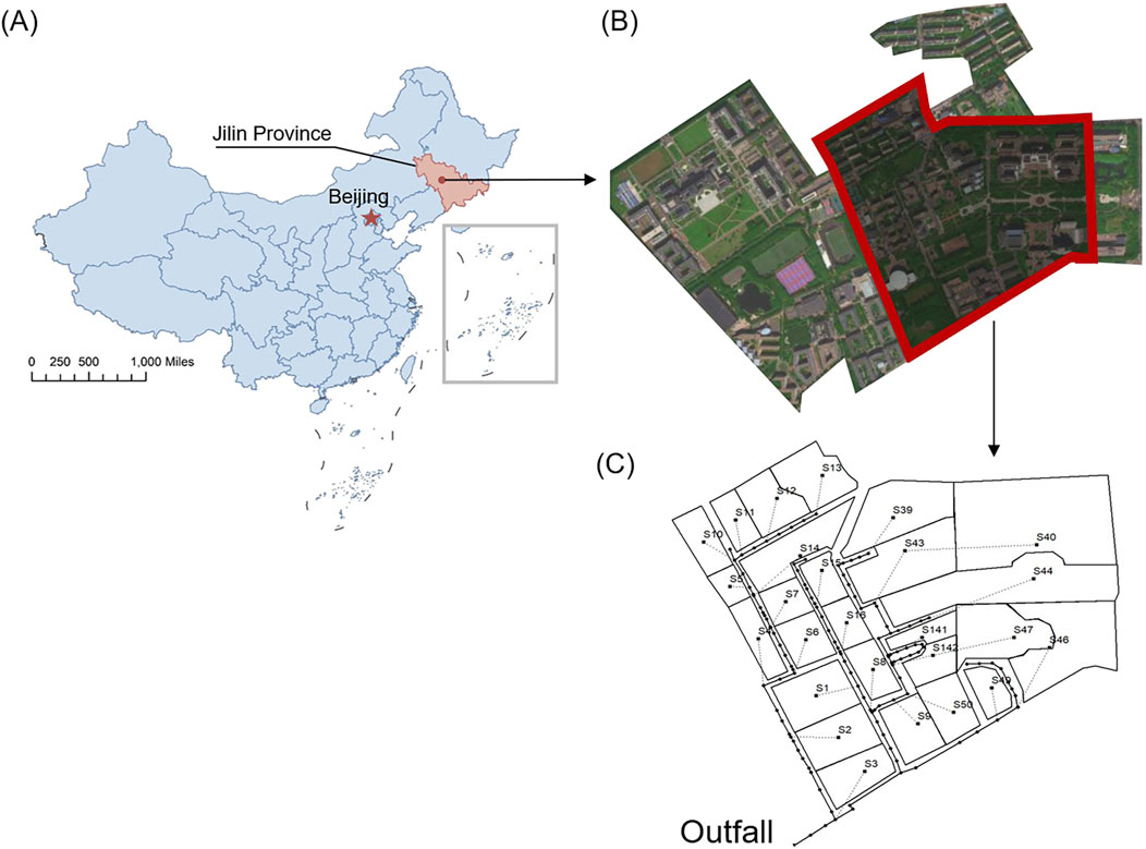
Figure 1. Study area overview (A) central campus of jilin university (B) sub-catchment delineation (C) drainage network layout.

The study area covers approximately 647,300 m² and has a complete drainage network. Based on the terrain and watershed network layout, the study area is divided into 26 sub-catchment areas (Figure 1; Table 1), with the underlying surface morphology identified using regional remote sensing data. The rain event of August 14 to 15, 2023 was selected for calibration (Figure 2A) with a return period of 0.11 years. The model validation was based on the rain event on 25 August 2023 (Figure 2B) with a return period of 0.13 years. Both rainfall events occurred during the flood season (June to September) in northern China. According to SWMM’s generalization requirements, better forecasting accuracy is achieved when the future application environment aligns with the model’s calibration period (Choi et al., 2002).

Table 1

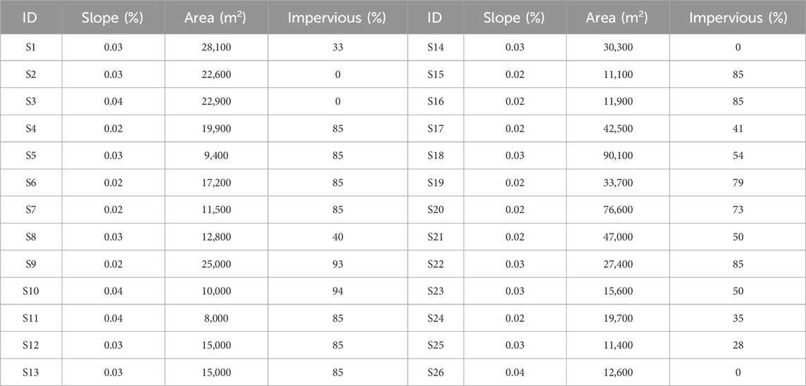
Table 1. Sub-catchments properties.

Figure 2

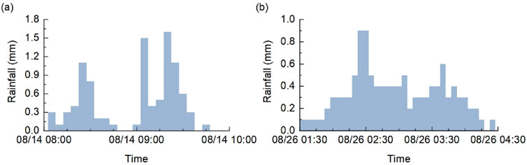
Figure 2. Rainfall process (a) August 14 to 15, 2023 (b) 25 August 2023.

1.2 Method

1.2.1 Latin hypercube sampling algorithm

McKay et al. proposed LHS algorithm in 1979, which was a stratified sampling method of taking approximately random samples from a multivariate distribution (Mckay et al., 1979).

For a random variable $X$, with its sample denoted as $x_i$, $i=1,2,\dots \dots ,I$, where $I$ is the dimension of the random variable $X$, the values $x_i$ are uniformly sampled from each value range ${∆}_i$, resulting in $J$ groups, This can be expressed as: $x_{i,j}=\left\{x_{1,j}\in {∆}_1,x_{2,j}\in {∆}_2,\dots ,x_{i,j}\in {∆}_i,\dots ,x_{I,j}\in {∆}_I\right\}$ and $p_{i,j}=\left\{x_{i,j}\in {\mathrm{\Omega }}_i,i=1,2,\dots \dots ,I,j=1,2,\dots \dots ,J\right\}$. In this paper, LHS algorithm was used to generate the sample set of model parameters.

1.2.2 Sensitivity analysis-back propagation method

In this paper, sensitivity analysis was used for key parameter identification to determine the main runoff generation pattern (Xie et al., 2021). Sensitivity analysis is an analytical technique to quantify the extent to which changes in independent variables lead to changes in dependent variables (Pan et al., 2021).

When the independent variable is $x_1,x_2,\dots ,x_n$ and the dependent variable is $y$, the mapping relationship between them is $y=f\left(x_1,x_2,\dots ,x_n\right)$. Each independent variable $x_i$ changes within its range, and the impact of these changes on the dependent variable $y$ is analyzed. This is referred to as the sensitivity of $y$ to the independent variable $x_i$. In this study, the SA-BP method, a global sensitivity analysis technique based on backpropagation neural networks, is used to simulate the complex nonlinear mapping relationship between rainfall and runoff in SWMM, considering the coupling effects of other model parameters (Li et al., 2014; Li et al., 2012).

1.2.3 Self-organizing map

In this paper, the SOM algorithm was used for optimizing the parameter range. The SOM was developed by the Finnish scientist T. Kohonen (Kohonen, 1998). The SOM algorithm is a neural network algorithm based on unsupervised learning that can achieve intelligent clustering of data through self-organizing competitive learning without understanding the interrelationships between sample data. The algorithm evaluates the similarity of input patterns using Euclidean distance, where a smaller distance indicates higher similarity, and clustering analysis can be performed based on a constant distance threshold.

The SOM process involves several key steps: First, the weight vectors of neurons are unitized. Then, the neuron most similar to the input vector is identified. Afterward, the weight vector of the winning neuron is adjusted using either the summation or subtraction method, where the weight vectors of other neurons remain unchanged. The adjustment is made using a learning rate that decreases over time. Through multiple adjustments, the winning neuron’s weight vector moves closer to the input vector.

1.2.4 Generalized likelihood uncertainty estimation and evaluation index

GLUE was used to analyze the parameter uncertainty of SWMM. The model calibration was essentially updating the parameters to reduce the model error to meet the design requirements. GLUE, a method of assessing the overall uncertainty of a model, was developed by the British hydrologist Beven based on the Generalized Sensitivity Analysis (RSA) method of Beven and Freer (2001), Hornberger and Spear (1980).

1.2.5 SWMM principle and structure

There are two types of surface runoff generation patterns used in the SWMM model, the permeable generation pattern and the impermeable generation pattern, as shown in Figure 3 The two types of runoff generation patterns are similar in principle. Each sub-catchment is treated as a non-linear “reservoir,” with rainfall and surface runoff from the upstream sub-catchment as the water input. The outflow consists of evaporation and surface runoff, with the presence or absence of infiltration determined by the sub-catchments underlying surface permeability. Surface runoff $Q$ will only occur if the reservoir depth $d$ exceeds the maximum depression storage depth $d_p$.

Figure 3

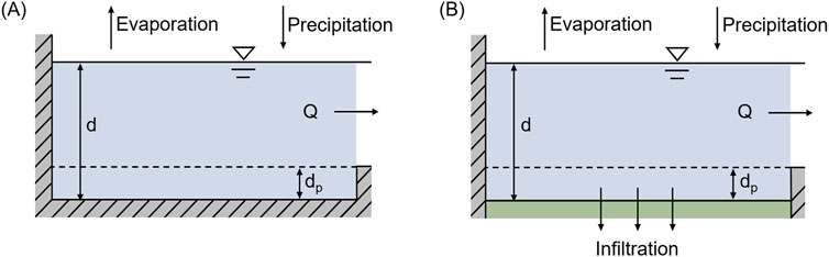
Figure 3. Conceptual view of surface runoff (A) impervious area (B) pervious area.

The parameters that dominate various land covers would be different, as they acted on different runoff generation patterns. To investigate the effect of each parameter on different runoff generation patterns, the simulation results were analyzed and discussed in different scenarios of varying impervious percentages.

2 SWMM parametric intelligent calibration method

2.1 Optimization of SWMM parameter ranges

In this study, 9 SWMM model parameters for the investigated watershed were optimized, denoted as $P$ (Figure 4). The LHS algorithm was employed to generate a sample set of 500 model parameters, denoted as $p_{i,j}$, where $p_{i,j}=\left\{p_{i,j}\in {\mathrm{\Omega }}_i;i=1,2,\dots \dots ,9;j=1,2,\dots \dots ,500\right\}$. SWMM was run to simulate the runoff process set based on $p_{i,j}$ groups parameter set. The parameters were randomly sampled within their respective value ranges ${\mathrm{\Omega }}_i$ (Rossman, 2015). The Nash-Sutcliffe efficiency (NSE) coefficient was chosen as the evaluation index of the model accuracy. The P-factor and R-factor were selected for evaluating the model uncertainty. The P-factor represents the ratio of the number of observation data points within the 95% confidence interval of the simulated values to the total number of observation data points, and the R-factor represents the ratio of the mean difference between the results corresponding to the 97.5% and 2.5% percentiles, i.e., expanding the upper and lower limits of the 95% confidence interval by 2.5%, to the standard deviation of the observation values (Narsimlu et al., 2013).

Figure 4

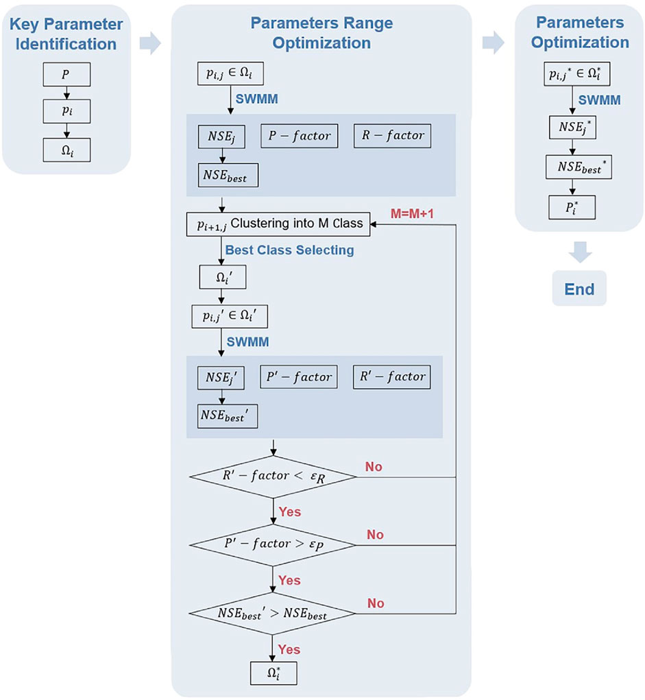
Figure 4. Framework flowchart.

To optimize the parameter ranges and improve the accuracy of the model simulation, the SOM was used as an intelligent clustering algorithm to perform a clustering analysis of the parameter values. The sampling set $p_{i+1,j}$ (10 dimensions) consisting of 500 parameter sets (9 dimensions) and corresponding simulation results, denoted as ${NSE}_j$. The highest ${NSE}_j$ is represented as ${NSE}_{best}$ (${NSE}_{best}=\mathit{max}\left\{{NSE}_j\right\}$). The SOM model classifies $p_{i+1,j}$ into 4, 5, and 6 clusters based on the corresponding NSE values (Figures 5–7).

Figure 5

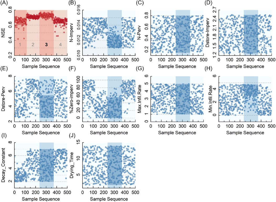
Figure 5. SOM 4-class clustering (A) NSE (B) N-Imperv (C) N-Perv (D) Dstore-Imperv (E) Dstore-Perv (F) %Zero-imperv (G) Max.Infil.Rate (H) Min.Infil.Rate (I) Decay_Constantv (J) Drying_Time.

Figure 6

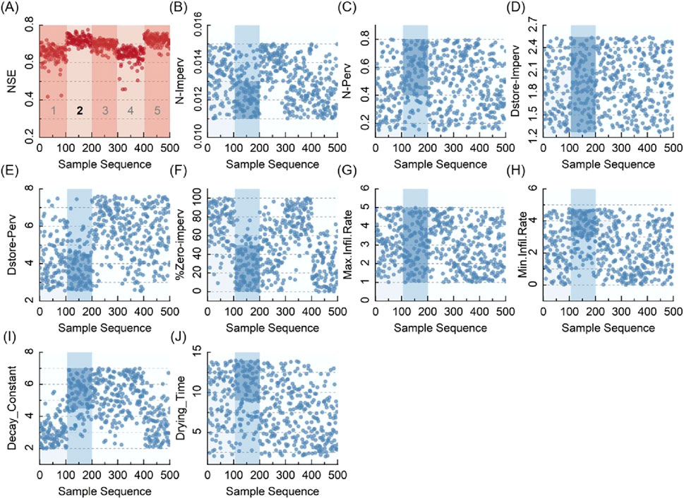
Figure 6. SOM 5-class clustering (A) NSE (B) N-Imperv (C) N-Perv (D) Dstore-Imperv (E) Dstore-Perv (F) %Zero-imperv (G) Max.Infil.Rate (H) Min.Infil.Rate (I) Decay_Constantv (J) Drying_Time.

Figure 7

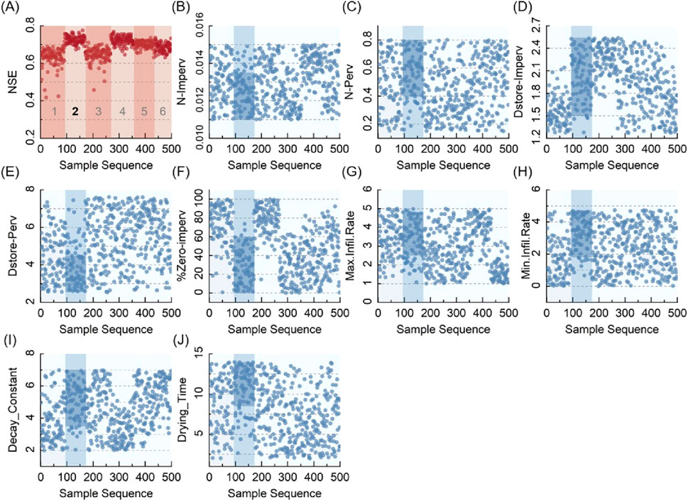
Figure 7. SOM 6-class clustering (A) NSE (B) N-Imperv (C) N-Perv (D) Dstore-Imperv (E) Dstore-Perv (F) %Zero-imperv (G) Max.Infil.Rate (H) Min.Infil.Rate (I) Decay_Constantv (J) Drying_Time.

The best class in terms of the high NSE coefficient and the low standard deviation was picked. The range of each parameter within this class was then considered to be optimized. As the number of clustering classes increased (e.g., from 4 to 6), the ranges of the parameter value were continuously narrowed down and then optimized. By comparing the NSE coefficients of the 4 classes in Figure 5A, the third class with the high NSE coefficients and the low standard deviation was chosen as the optimal one. The parameter ranges corresponding to the optimal class were extracted as the new ranges for the next round of optimization (Figures 5B–J). The N-Imperv in Figure 5B could be used as an example; The parameter values of the third class were concentrated to the optimal range of [0.011, 0.0125] after the 4-class clustering. Similarly, the ranges of values for the parameters Dstore-Perv (Figure 5E), %Zero-imperv (Figure 5F), and Min. Infil.Rate (Figure 5H) can be reduced. The remaining parameters (Figures 5C, D, G, I, J) had no narrower concentration so the initial ranges of their values were still used. The value ranges of each parameter after the clustering according to 4, 5, and 6 classes were shown in Table 2, and the optimized parameter ranges were the intersection of the three clustering results.

Table 2

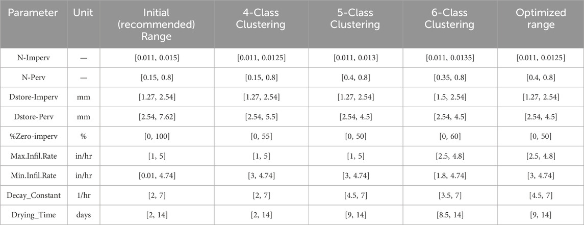
Table 2. The parameters range under clustering of groups.

Figure 8 shows the degrees to which the parameter ranges were reduced. Except for Dstore-Imperv, all parameters have been reduced significantly, with the largest reduction of 63.2% for Max. Infil.Rate and an average reduction of 47.4% for all parameters.

Figure 8

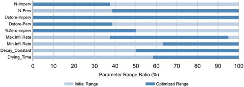
Figure 8. Comparison of parameter ranges before and after the optimization.

In the next iteration, the LHS algorithm is used again to generate 500 parameter sets, denoted as ${p_{i,j}}^{\prime }$, from the optimized parameter ranges ${{\mathrm{\Omega }}_i}^{\prime }$ to drive the SWMM simulation.

In the next iteration, the LHS algorithm is used again to generate 500 parameter sets from the optimized parameter range ${{\mathrm{\Omega }}_i}^{\prime }$ denoted as ${p_{i,j}}^{\prime }$ to drive the SWMM simulation. This process yields a new ${{NSE}_j}^{\prime }$, ${{NSE}_{best}}^{\prime }$ (${{NSE}_{best}}^{\prime }=\mathit{max}\left\{{{NSE}_j}^{\prime }\right\}$), $P’-factor$ and $R’-factor$.

This cycle will be only ended until the optimal parameter ranges ${\mathrm{\Omega }}_i^{*}$ were found when the $P’-factor$, $R’-factor$, and the ${{NSE}_{best}}^{\prime }$ reached better values than the design requirements; otherwise, the SOM clustering algorithm would be repeated. After confirming ${{\mathrm{\Omega }}_i}^{*}$, the final optimal parameter set ${p_i}^{*}$ can be determined through computation.

2.2 Uncertainty analysis of model

Compared to the original 95% confidence interval (Figure 9), the updated 95% confidence interval became significantly narrower through the class clustering. There were also significant reductions in the standard deviation (by 49.39% on average), discrete coefficient (SD/Mean) (by 48.77% on average), and the R-factor from 0.396 to 0.226 of the optimized parameters set (Table 3). Although the NSE coefficients did not significantly improve (from 0.776 to 0.777), the effect of parameter uncertainty on the accuracy of model results was effectively mitigated.

Figure 9

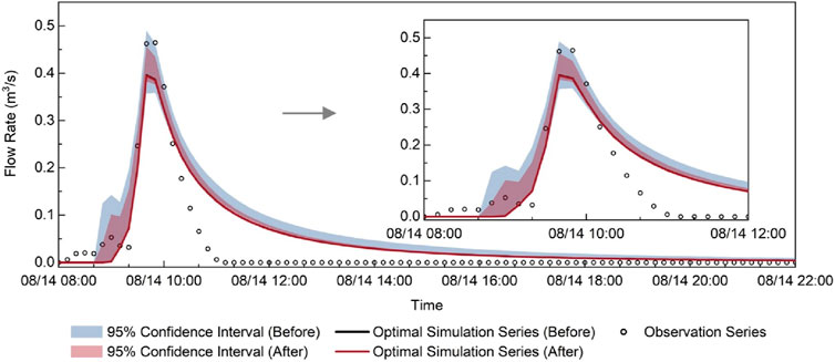
Figure 9. Confidence intervals for flow hydrograph before and after parameters range optimization.

Table 3

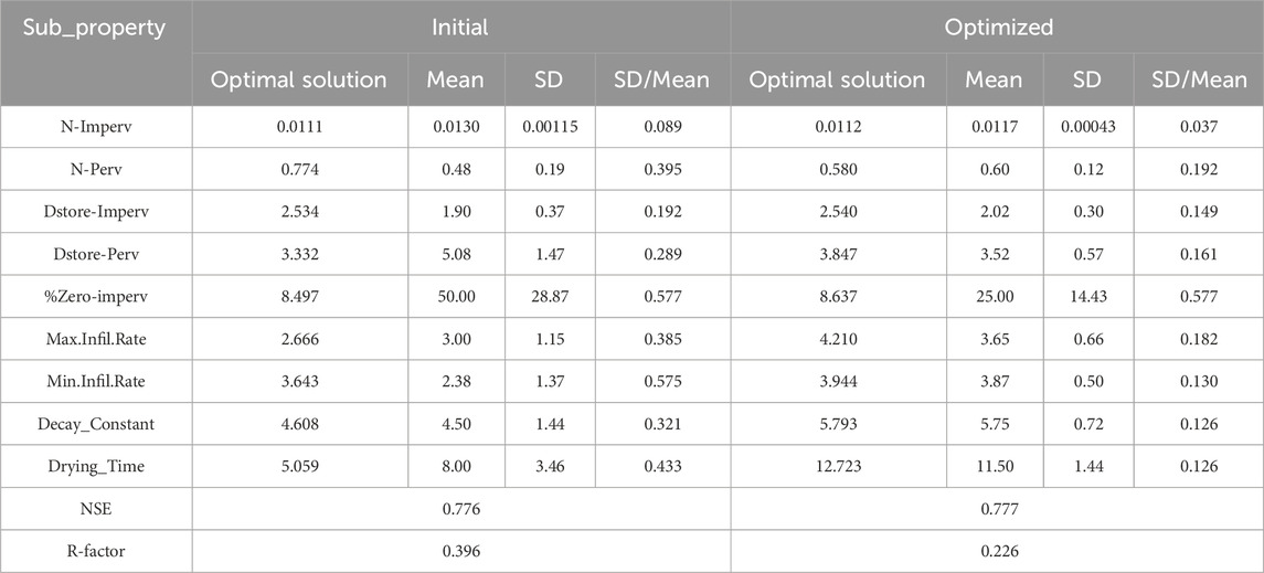
Table 3. Statistical characteristics and optimal solution of parameters set before and after parameters range optimization.

2.3 Evaluation of optimization accuracy

Evaluation of the accuracy of the simulation and validation results was carried out based on the above parameter optimization results. The results (see Table 3, the Optimal Solution) were validated by selecting the return period of 0.13 years of rainfall on 25 August 2023 (Figure 10). It can be seen that the NSE coefficient remained high after the parameter optimization, indicating that the parameter optimization method was effective and feasible.

Figure 10

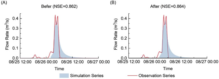
Figure 10. Validation period flow hydrograph (A) Before parameter optimization (B) After parameter optimization.

3 Factors controlling the runoff generation patterns

As can be seen from Table 3, although the optimization of parameter range was effective in abating the model uncertainty, there was no significant improvement in the model accuracy. According to the SWMM model runoff analysis, the impermeable area and its runoff generation patterns were likely to be the main cause controlling the runoff simulation. The runoff pattern was only related to the three parameters in this study: N-Imperv, Dstore-Imperv, and %Zero-imperv, which were relatively easy to determine. In order to verify this assumption, the key parameters were identified according to the land covers, while the runoff generation patterns were analyzed with various surface characteristics such as impervious percentages of subcatchments.

3.1 Identification of runoff generation patterns

The SA-BP Sensitivity Analysis was used to identify the key parameters that controlled the runoff generation patterns (Chen et al., 2009; Jenkins, 2006). The LHS algorithm was used to generate 500 sets of samples as the model inputs, and the NSE coefficients corresponding to the simulation results were used as the outputs. Three runs were performed and the results of each run, i.e., the sensitivity of these parameter sets, were normalized separately, shown in Figure 11. The influence of the parameters %Zero-imperv on the simulation results was greater than the other parameters with the current surface conditions. It can be inferred that the impermeable runoff generation pattern was the major factor controlling the runoff generation pattern due to the greater proportion of impermeable area (55.8%).

Figure 11

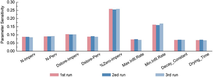
Figure 11. Parameter sensitivity analysis under current surface conditions.

3.2 Urban runoff generation mechanisms

The above analysis shows that when the impermeable area was 55.8%, the parameters controlling the impermeable surface played a predominant role in determining the runoff generation process, which needed to be further studied to fully understand the underlying relationship between the imperviousness of the catchment and the SWMM accuracy.

3.2.1 Impervious scenarios

The model impervious percentages of 0%, 10%, 20%, 90%, and 100% were studied separately to investigate their roles in affecting the runoff generation patterns. The rain event on August 14 to 15, 2023 was selected as the model input to simulate the corresponding hydrographs at the outfall (Figure 12). As the percentage of impervious area increased, the peak and total runoff significantly increased as expected, and the magnitude of change decreased with the increase of impervious area.

Figure 12

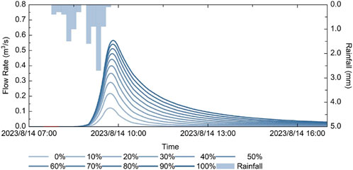
Figure 12. Hydrographs at the outfall for different impermeable percentages.

3.2.2 Identification of the control parameters

To identify the key parameters controlling the runoff generation patterns, the sensitivity analysis based on the SA-BP method was performed for the parameters in each impermeable scenario. The results were normalized (Figure 13A) and sorted (Figure 13B). When all the catchment surface was permeable, the parameter Min. Infil.Rate was the key parameter affecting the runoff generation, followed by N.Perv and Decay_Constant. these three parameters were all acting on the permeable generation pattern, i.e., the runoff generation process of the catchment was mainly controlled by the permeable pattern. When the entire catchment was covered by the impermeable surface, the parameter %Zero.Imperv was the key parameter, followed by N. Imperv and Dstore-Imperv; all three parameters were acting on the impermeable surface, i.e., the impermeable pattern was dominant in determining the runoff generation.

Figure 13

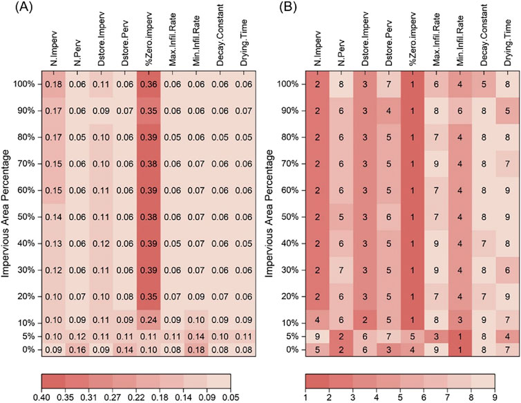
Figure 13. Parameter sensitivity at different impervious area percentages (A) normalized indicators (B) indicators sorting.

As the percentages of impervious area in the study area increased, the sensitivity of parameters representing the impervious surface increased according and vice versa for the parameters controlling the permeable surface (Figure 13A), which indicates that the runoff generation mechanism gradually shifted from the permeable pattern to the impermeable pattern. Notably, 20% of the impermeable percentage was the threshold of determining the surface runoff generation pattern; when the impervious percentage became less than 10%, Min. Infil.Rate became the key parameter and the runoff generation process was controlled by the permeable pattern; when the impervious percentage was greater than 10%, the key parameter became %Zero.imperv and the runoff generation process was impermeable pattern.

The value of this study was to qualitatively estimate the simulation and forecasting accuracy of the model based on the percentage of the impermeable area, so that the requirements of the simulation accuracy could be reasonably proposed. When the impervious percentage exceeded a certain critical value such as 10% in this study, the SWMM could have a good simulation accuracy; conversely, the accuracy may not be too good, so the accuracy requirement should be set relatively lower in practical application.

4 Conclusion

This study used the SOM and GLUE algorithms for the clustering analysis to optimize the parameter range and effectively reduce the model uncertainty. This method was used for the 9 parameters of SWMM and the ranges of the 8 parameters were significantly reduced, except for the parameter Dstore-Imperv. The largest reduction in the value range by 63.2% was achieved for the parameter Max. Infil.Rate, with an average reduction rate of 47.4% for all parameters.

This work provided a feasible 3-step workflow for SWMM calibration consisting of identifying key parameters by the SA-BP method, optimizing the parameter ranges by the SOM method, and optimizing the parameter values based on the LHS method.

The SWMM runoff generation pattern was found to be controlled by the ratio of permeable area to the impermeable area of the underlying surface based on this study. When the impervious area accounted for over 10%, the corresponding parameters of the impervious surface controlled the runoff generation pattern of the catchment, and the accuracy of SWMM results tended to be relatively higher; on the contrary, if the overall impervious percentage was below 10%, the runoff generation was controlled by the permeable pattern, and the accuracy of SWMM results was comparatively lower.

Given that a universal parameter calibration tool for SWMM has not yet been developed, the parameter range optimization and calibration method based on the SOM algorithm proposed in this paper not only improves the accuracy of SWMM simulation and prediction but also provides additional value in the following aspects: Firstly, by establishing reasonable value ranges for each parameter and gradually increasing the number of parameters set classifications (e.g., dividing the parameter set into 4, 5, and 6 categories in this study), the parameter ranges are continuously narrowed to achieve parameter optimization, thereby reducing the uncertainty in parameter values and their combinations. Secondly, by identifying key parameters, the dominant runoff generation pattern can be determined, which further allows the quantification of the critical impervious area ratio at which the “impermeable generation pattern” becomes the dominant runoff generation pattern (e.g., 10% in this study). At this point, SWMM tends to achieve higher simulation and prediction accuracy, and most urban rainfall-runoff patterns fall into this category. Conversely, when the “permeable generation pattern” is the dominant runoff generation pattern, the simulation and prediction accuracy of SWMM tends to be relatively lower. This often occurs in catchments with significant spatial variability in underlying surface conditions.

The SWMM parameter calibration in this study was conducted based on measured historical rainfall and runoff data. The Python-based SWMM batch computation program, combined with LHS, was used to generate SWMM accuracy indicators such as NSE. The SOM clustering algorithm was then applied to optimize parameter value ranges and obtain the optimal parameter combination. The complete execution of the case study in this paper takes approximately within 2 h. If this algorithm were embedded into an urban flood control system for real-time simulation and forecasting, it would involve system integration and other related aspects. This will be the focus of the authors’ future work.

The results of this study have significant potential applications in urban hydrology and flood risk management. The proposed workflow improves both the calibration efficiency and accuracy of SWMM, thereby enhancing its suitability for urban stormwater simulation. Furthermore, a deeper understanding of runoff generation mechanisms contributes to optimizing urban drainage system design and improving the accuracy of flood predictions. Looking ahead, this approach can be extended to real-time flood control, urban hydrological digital twin modeling, and integrated water resource management.

Data availability statement

The datasets presented in this study can be found in online repositories. The names of the repository/repositories and accession number(s) can be found in the article/supplementary material.

Author contributions

ZY: Conceptualization, Data curation, Formal Analysis, Investigation, Methodology, Resources, Validation, Visualization, Writing–original draft, Writing–review and editing. JL: Methodology, Writing–review and editing. YF: Conceptualization, Methodology, Writing–original draft, Writing–review and editing. JW: Methodology, Writing–review and editing. HW: Methodology, Writing–review and editing. CL: Formal Analysis, Writing–review and editing.

Funding

The author(s) declare that financial support was received for the research and/or publication of this article. This study was supported by Chinese National Key Research and Development Program (No. 2022YFC3090600), the Research Fund of the State Key Laboratory of Simulation and Regulation of Water Cycle in River Basin (Grant No. SKL2022TS11) and the Open Research Fund of Key Laboratory of River Basin Digital Twinning of Ministry of Water Resources.

Conflict of interest

The authors declare that the research was conducted in the absence of any commercial or financial relationships that could be construed as a potential conflict of interest.

Generative AI statement

The author(s) declare that no Generative AI was used in the creation of this manuscript.

Publisher’s note

All claims expressed in this article are solely those of the authors and do not necessarily represent those of their affiliated organizations, or those of the publisher, the editors and the reviewers. Any product that may be evaluated in this article, or claim that may be made by its manufacturer, is not guaranteed or endorsed by the publisher.

References

Abbaspour, K. C., Yang, J., Maximov, I., Siber, R., Bogner, K., Mieleitner, J., et al. (2007). Modelling hydrology and water quality in the pre-alpine/alpine Thur watershed using SWAT. J. Hydrology 333, 413–430. doi:10.1016/j.jhydrol.2006.09.014

CrossRef Full Text | Google Scholar

Ajami, N. K., Gupta, H., Wagener, T., and Sorooshian, S. (2004). Calibration of a semi-distributed hydrologic model for streamflow estimation along a river system. J. Hydrology 298, 112–135. doi:10.1016/j.jhydrol.2004.03.033

CrossRef Full Text | Google Scholar

Bellos, V., Kourtis, I. M., Moreno-Rodenas, A., and Tsihrintzis, V. A. (2017). Quantifying roughness coefficient uncertainty in urban flooding simulations through a simplified methodology. Water 9, 944. doi:10.3390/w9120944

CrossRef Full Text | Google Scholar

Beven, K., and Freer, J. (2001). A dynamic TOPMODEL. Hydrol. Process. 15, 1993–2011. doi:10.1002/hyp.252

CrossRef Full Text | Google Scholar

Chen, Q., Guo, W., and Li, C. (2009). “Railway passenger volume forecast by GA-SA-BP neural network,” in International workshop on intelligent systems and applications, ISA 2009.

Google Scholar

Chen, R., Wang, Y., Li, G., Yan, D., and Cao, H. (2023). “Pre-training models based knowledge graph multi-hop reasoning for smart grid technology,” in Lecture notes in electrical engineering. Editors Z. REN, Y. HUA, and M. WANG (Springer Science and Business Media Deutschland GmbH), 1866–1875.

Google Scholar

Choi, K.-S., and Ball, J. E. (2002). “A generic calibration approach: monitoring the calibration,” in Water challenge: balancing the risks: hydrology and water resources symposium 2002. Editor A. C. T. Barton (Australia: Institution of Engineers).

Google Scholar

GarzóN, A., Kapelan, Z., Langeveld, J., and Taormina, R. (2022). Machine learning-based surrogate modeling for urban water networks: review and future research directions. Water Resour. Res. 58, e2021WR031808. doi:10.1029/2021wr031808

CrossRef Full Text | Google Scholar

Hornberger, G. M., and Spear, R. C. (1980). Eutrophication in peel inlet—I. The problem-defining behavior and a mathematical model for the phosphorus scenario. Water Res. 14 (1), 29–42. doi:10.1016/0043-1354(80)90039-1

CrossRef Full Text | Google Scholar

Huang, C.-L., Hsu, N.-S., Wei, C.-C., and Luo, W.-J. (2015). Optimal spatial design of capacity and quantity of rainwater harvesting systems for urban flood mitigation. Water 7, 5173–5202. doi:10.3390/w7095173

CrossRef Full Text | Google Scholar

Jafari, F., Mousavi, S. J., Yazdi, J., and Kim, J. H. (2018). Real-time operation of pumping systems for urban flood mitigation: single-period vs. Multi-period optimization. Water Resour. Manag. 32, 4643–4660. doi:10.1007/s11269-018-2076-4

CrossRef Full Text | Google Scholar

Jenkins, W. M. (2006). Neural network weight training by mutation. Comput. Struct. 84, 2107–2112. doi:10.1016/j.compstruc.2006.08.066

CrossRef Full Text | Google Scholar

Kohonen, T. (1998). The self-organizing map. Neurocomputing 21, 1–6. doi:10.1016/s0925-2312(98)00030-7

CrossRef Full Text | Google Scholar

Li, H., Tian, Q., Wang, X., and Wu, Y. N. (2014). Multivariate coupling sensitivity analysis method based on a back-propagation network and its application. J. Hydrologic Eng. 20, 06014013. doi:10.1061/(asce)he.1943-5584.0001131

CrossRef Full Text | Google Scholar

Li, H., Xie, M., and Jiang, S. (2012). Recognition method for mid-to long-term runoff forecasting factors based on global sensitivity analysis in the Nenjiang River Basin. Hydrol. Process. 26, 2827–2837. doi:10.1002/hyp.9211

CrossRef Full Text | Google Scholar

Li, H., Zhang, C., Chen, M., Shen, D., and Niu, Y. (2023). Data-driven surrogate modeling: introducing spatial lag to consider spatial autocorrelation of flooding within urban drainage systems. Environ. Model. and Softw. 161, 105623. doi:10.1016/j.envsoft.2023.105623

CrossRef Full Text | Google Scholar

Mckay, M. D., Beckman, R. J., and Conover, W. J. (1979). Comparison of three methods for selecting values of input variables in the analysis of output from a computer code. Technometrics 21, 239–245. doi:10.1080/00401706.1979.10489755

CrossRef Full Text | Google Scholar

Narsimlu, B., Gosain, A. K., and Chahar, B. R. (2013). “Model calibration and uncertainty analysis for runoff in the upper sind River Basin, India, using sequential uncertainty fitting,” in World environmental and water resources congress 2013: showcasing the future.

Google Scholar

Pan, L., NováK, L., Lehký, D., NováK, D., and Cao, M. (2021). Neural network ensemble-based sensitivity analysis in structural engineering: Comparison of selected methods and the influence of statistical correlation. Comput. and Struct. 242, 106376. doi:10.1016/j.compstruc.2020.106376

CrossRef Full Text | Google Scholar

Rossman, L. A. (2015). Storm water management model (SWMM) version 5.1 user's manual. The United States of America: United States Environmental Protection Agency.

Google Scholar

Serban, R., and Freeman, J. S. (2001). Identification and identifiability of unknown parameters in multibody dynamic systems. Multibody Syst. Dyn. 5, 335–350. doi:10.1023/A:1011434711375

CrossRef Full Text | Google Scholar

Snieder, E., and Khan, U. T. (2022). “Investigating event selection for GA-based SWMM rainfall-runoff model calibration,” in Lecture notes in civil engineering. Editors S. Walbridge, M. Nik-Bakht, K. T. Ng, M. Shome, M. S. Alam, A. El Damattyet al. (Springer Science and Business Media Deutschland GmbH), 429–441.

Google Scholar

Sun, H., Dong, Y., Lai, Y., Li, X., Ge, X., and Li, C. (2022). The multi-objective optimization of low-impact development facilities in shallow mountainous areas using genetic algorithms. Water 14, 2986. doi:10.3390/w14192986

CrossRef Full Text | Google Scholar

Wagner, B., Reyes-Silva, J. D., FöRSTER, C., Benisch, J., Helm, B., and Krebs, P. (2019). “Automatic calibration approach for multiple rain events in SWMM using Latin Hypercube sampling,” in New trends in urban drainage modelling.

Google Scholar

Xie, K., Liu, P., Zhang, J., Wang, G., Zhang, X., and Zhou, L. (2021). Identification of spatially distributed parameters of hydrological models using the dimension-adaptive key grid calibration strategy. J. Hydrology 598, 125772. doi:10.1016/j.jhydrol.2020.125772

CrossRef Full Text | Google Scholar

Yang, Y., Li, Y., Huang, Q., Xia, J., and Li, J. (2023). Surrogate-based multiobjective optimization to rapidly size low impact development practices for outflow capture. J. Hydrology 616, 128848. doi:10.1016/j.jhydrol.2022.128848

CrossRef Full Text | Google Scholar

Zhao, L. X., Li, H. Y., Li, C. H., Zhao, Y. L., Du, X. Q., Ye, X. Y., et al. (2024). Enhanced SWAT calibration through intelligent range-based parameter optimization. J. Environ. Manag. 367, 121933. doi:10.1016/j.jenvman.2024.121933

PubMed Abstract | CrossRef Full Text | Google Scholar

Zhong, B., Wang, Z., Yang, H., Xu, H., Gao, M., and Liang, Q. (2022). Parameter optimization of SWMM model using integrated morris and GLUE methods. Water 15, 149. doi:10.3390/w15010149

CrossRef Full Text | Google Scholar