 Harry D. Kambezidis
- 1Institute of Environmental Research and Sustainable Development, National Observatory of Athens, Lofos Nymphon, Athens, Greece
- 2Laboratory of Soft Energioes Applications and Environmental Protection, Department of Mechanical Engineering, University of West Attica, Aigaleo, Greece
Solar radiation comprises the primary renewable source of energy on Earth and has so been exploited in the last 20 years. Despite this, solar radiation measurements are scarce worldwide, thus giving space to modelling. Nevertheless, modelling solar radiation at an hourly level is nowadays required for a short-term output forecast from solar installations. The daily global solar radiation decomposition models are one category of solar models that convert daily solar radiation values to hourly ones. The Collares-Pereira and Rabl (CPR) and Collares-Repeira, Rabl and Gueymard (CPRG) models have shown to provide a better performance than others at individual sites without exhibiting any sign of universality on the other hand. The current study looks at this gap. In this regard, twelve sites are selected around the world. To estimate hourly values, the CPR and CPRG models are applied to daily solar radiation estimates for each site in particular years. Hourly data sets that are openly accessible provide the daily values. Additionally, daily and monthly values are derived from the estimated and observed hourly values. The hourly, daily, and monthly scales are used to compare the two models’ performances. The CPR model outperforms the CPRG model across all sites and time scales. A universal coefficient of correction is used to further enhance the CPR performance, bringing the CPR-estimated solar radiation very close to the observed one.
1 Introduction
Solar energy is the primary source on Earth for controlling various fields such as the atmospheric environment (Giesen et al., 2008), terrestrial climate (Larsen et al., 2007), and terrestrial ecosystems (Bojinski et al., 2014). The abundance of solar radiation on Earth also makes it the most significant renewable energy source. As a result, it has been used in a variety of solar energy applications, primarily in the form of photovoltaic (PV) energy, such as (Kambezidis, 2021; Kambezidis, 2022). The substantial contribution that solar radiation makes to the Earth’s thermal (energetic) balance is another crucial function. The hydrological cycles employed for irrigation, agriculture, and water-resource management are impacted by this equilibrium in terms of evapotranspiration (Boscaini et al., 2020). For these reasons, the knowledge of solar radiation availability at a location is important. Furthermore, using solar energy requires this kind of understanding (Khatib et al., 2012). However, even now, there is a lack of data based on surface solar radiation measurement stations (Kambezidis, 2022). This disadvantage has long since made the creation of models of solar radiation necessary.
The models may be statistical procedures (e.g., heuristic, fuzzy logic), mathematical formulations (e.g., linear, polynomial), or artificial intelligence (e.g., artificial neural networks, generalised regression, feedback-back forward, cascade-forward back-propagation, neuro-fuzzy, and optimised ANNs) (Kambezidis, 2022; Khatib et al., 2012). The purpose of the models is to synthesise solar radiation time series in locations without solar data availability. Predicting the short-term (few hours ahead) solar radiation at a place is another goal, particularly for the AI-based models. This short-term knowledge is highly significant for the market of renewable energy (Nwokolo et al., 2022).
Hourly readings are crucial for solar modelling assessments or in-depth analyses of the solar availability at the site of interest, even though many meteorological stations worldwide now record horizontal solar radiation on a daily basis (Kambezidis, 2022). With the intention of providing hourly values of global horizontal solar radiation in conjunction with meteorological records or to fill in gaps, the so-called daily global solar radiation decomposition (DGSRD) models (Yao et al., 2015) were developed back in the 1950s, for example Whillier (1956). Depending on the input parameters that are employed, the DGSRD models are separated into two groups. Solar geometry (i.e., solar hour angle, solar declination, day length, and time, either local or solar) is used in the first category. Whillier’s work is a typical example (Whillier, 1956). Liu and Jordan (1960), Collares-Pereira and Rabl (1979), Gueymard (1986), which is a modification of the CPR, although this latter researcher later developed an own model (Gueymard, 2000), Garg and Garg (1987), and Newell (1983) are other models of this type. The second group comprises models that utilise the Gaussian function, including representative models created by Jain (1984), Jain (1988), Baig et al. (1991), El shazly (1996).
Using data from specific sites, the accuracy of the aforementioned DGSRD models has been demonstrated. These sites include four in South Africa (Whillier, 1956), one in the United States (Liu and Jordan, 1960), five in the United States (Collares-Pereira and Rabl, 1979), one in Canada (Gueymard, 1986; Gueymard, 2000), four in India (Garg and Garg, 1987), one in the United States (Newell, 1983), one in Italy (Jain, 1984), one in Canada (Jain, 1988), one in Pakistan (Baig et al., 1991), and one in Egypt (El shazly, 1996). All of these studies have looked at data from one or more sites in a single country, with the exception of the work by Gueymard (2000), which collected data from 135 locations worldwide to develop and assess his own model. However, none of these studies have assessed the most popular DGSRD models of categories 1 and 2 using global data and drawn conclusions regarding their effectiveness. Therefore, bridging this gap is the goal of the current work. Only models that have demonstrated accuracy in the majority of research have been selected here for simplicity’s sake; the CPR and CPRG models satisfy the requirements, as demonstrated by Yao et al. (2015). Thus, these two DGSRD models have been considered in the current work.
The article is divided into sections. Section 2 deploys the data and methodologies used. Section 3 provides the results of the study. Section 4 gives the conclusions of the work and discusses its main achievements, while it refers to future work in order to expand the efficiency of the models. A nomenclature is also deployed to provide a summary of the abbreviations and main symbols used in the study. Acknowledgements and references follow.
2 Materials and methods
2.1 Data collection
To implement the goals of the study, the same 12 sites around the world with those selected by Kambezidis et al. (2024) were used. The selection criteria were: different environmental characteristics (i.e., different climatological conditions), different terrain features (i.e., different topographical characteristics), and distribution across the continents (provided that available measurements exist). This way, all the climatological, terrain and distribution patterns are reflected in the solar radiation data. Table 1 shows the selected sites in alphabetical order together with their geographical coordinates, environmental description, climatological classification, and period of usable data, while Figure 1 provides a world map indicating the location of the 12 sites.
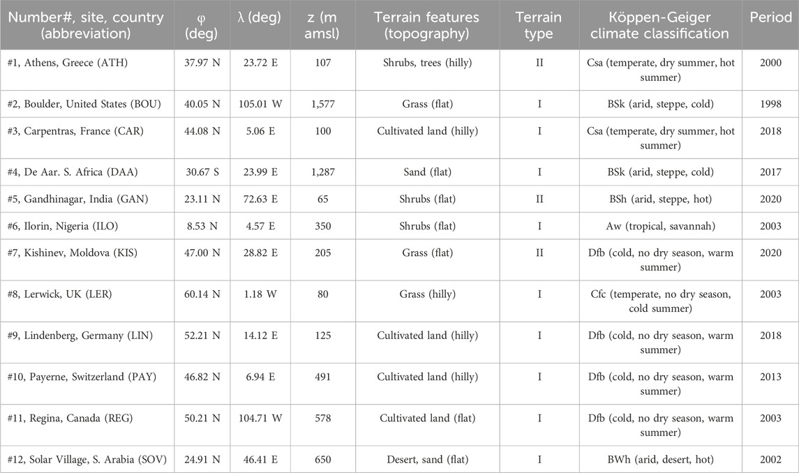
Table 1. The 12 selected sites of the present study in alphabetical order. The symbols φ, λ, and z denote the geographical latitude (positive degrees north of the Equator), the geographical longitude (positive degrees east of the Greenwich meridian), and the altitude of the site (amsl = above mean sea level), respectively. In column 6, I denotes rural, and II denotes urban environment. N = north, S = south, E = east, W = west. All geographical coordinates have been rounded to the second decimal digit.
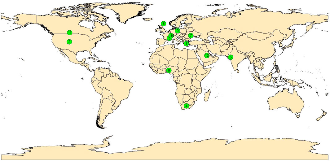
Figure 1. Location of the 12 selected sites (green circles). The circled numbers correspond to those in column 1 of Table 1. For the reader’s ease, 1 = ATH, 2 = BOU, 3 = CAR, 4 = DAA, 5 = GAN, 6 = ILO, 7 = KIS, 8 = LER, 9 = LIN, 10 = PAY, 11 = REG, and 12 = SOV.
For the purpose of the study, the global horizontal irradiance, Hg (in Wm-2), included in the data sets of Kambezidis et al. (2024) for the 12 sites, was also used. The selection of the sites and their solar radiation data were based on the BSRN (Baseline Surface Radiation Network), except for Athens (ATH); in this case, data from the Actinometric Station of the National Observatory of Athens (ASNOA) not belonging to BSRN was used. The abbreviations of the sites (except for Athens) are those provided by the BSRN typology. A description of the BSRN operation can be found in Driemel et al. (2018). All data was downloaded from the BSRN network on permission, except for the Athens data, which is part of the solar radiation components measured at ASNOA, Greece, in continuous operation since 1952.
As shown in Table 1, single years were selected for analysis at each site instead of a period of years. As mentioned in Kambezidis et al. (2024)“…That was performed on the rationale that no climatological analysis was intended to be conducted within the scope of this study … For this reason, the year for each site was selected in the period 1999 to 2020 from the BSRN list of stations, with an additional restriction that the individual years cover the mentioned period as broadly as possible. This way, any weather peculiarities occurring over an extended area within a specific year would be avoided.”
All data values are hourly averages. The BSRN network provides its data in UTC (universal time coordinated), while the data from ASNOA is in LST (local standard time). Therefore, a transformation of all UTC data into LST ones for the 12 sites, except ATH, took place in the data elaboration phase. In this stage, the corresponding solar hour angle, ω (positive degrees after solar noon, −180o ≤ ω ≤ 180o), solar altitude, γ (positive degrees above the local horizon, −90o ≤ γ ≤ 90o), solar azimuth, ψ (positive degrees after solar noon, −180o ≤ ψ ≤ 180o), and solar declination, δ (in degrees, −23.5o ≤ δ ≤ 23.5o) values over the selected year for each station were calculated by using the XRONOS.bas code (Kambezidis and Papanikolaou, 1990; Kambezidis and Tsangrassoulis, 1993), (xronos means time in Greek with x being spelled as ch). XRONOS.bas is an improvement to the original SUNAE code (Walraven, 1978). A discontinuity in the estimation of ψ at the sunrise and sunset moments was recently discovered and solved by providing an update version of XRONOS [XRONOS.ma in the Matlab environment (Kambezidis et al., 2022)]. For the purpose of the present work, the latest version of XRONOS was used to calculate the γ, ψ, and δ values at the 12 sites halfway between two consecutive hours (i.e., at n:30′ between hours n and n+1). Then, these values were assigned to the Hg value at the n+1 h. After completing these steps, a quality-control procedure took place over all the 12 data sets: values of Hg,h ≤ 0 Wm-2 were rejected; also no calculation was made for γ < 5o. The remaining hourly values on each day were summed up to give the daily ones in Whm-2.
2.2 Methodology
As mentioned in the Introduction, two specific DGSRD models are considered in the present analysis, i.e., the CPR and CPRG ones. Their mathematical formulations are the following.
2.2.1 The CPR model
where Hg,h and Hg,d are the hourly and daily solar radiation values in Wm-2 and Whm-2, respectively; rCPR is the ratio of hourly to daily global horizontal solar radiation (in h-1); ωss is the sunset solar hour angle (in degrees); φ is the geographical latitude of the site (positive degrees in the northern hemisphere); a, b are the constants of Equation 2.
2.2.2 The CPRG model
where rCPRG is the ratio of hourly to daily global horizontal solar radiation (in h-1); ωsr is the sunrise solar hour angle (in degrees); a, b are the constants of Equation 7.
2.2.3 Data processing
For each of the 12 sites, the hourly ratios rCPR and rCPRG were calculated from the expressions (Equations 2, 7) for the CPR and CPRG models, respectively. Then, the criteria mentioned in Section 2.1 were applied to the 12 data sets, which left 4527, 4757, 4858, 4719, 4547, 4540, 4831, 4964, 4852, 4910, 4724, and 4771 h free of errors on annual basis for the ATH, BOU, CAR, DAA, GAN, ILO, KIS, LER, LIN, PAY, REG, and SOV sites, respectively. After cleaning the data sets, a summation of the Hg,h hourly values for each day in the year corresponding to each site took place to derive the daily Hg,d values. The daily Hg,d values were afterwards multiplied by the hourly rCPR or rCPRG values of the same day to produce the estimated Hg,h values for the CPR and CPRG models, respectively. Annual and monthly values were also calculated for the observed and modelled Hg values at all the 12 sites. The same averaging process was applied to the rCPR and rCPRG hourly values; these monthly and annual r values in association with the corresponding Hg values were used to see if a better performance of the CPR and CPRG models could be achieved in terms of the statistical metrics discussed in the following Section. All solar radiation values refer to all-sky conditions.
2.2.4 Model performance
To evaluate the model-estimated values (i.e., the performance of the CPR and CPRG models) the following statistical metrics were considered: the root mean-square error (RMSE), the mean-bias error (MBE), the mean-absolute error (MAE), the coefficient of determination (R2), and the index of agreement (d). Further, a linear (or non-linear in some cases) regression analysis took place between the observed and estimated hourly, daily and monthly Hg values at the 99.9% confidence interval (CI). The formulations of the metrics are given below.
where Ei and Oi are the ith estimated and observed value, respectively; N is the total number of data points as deployed in Section 2.2.3 for the 12 sites. The RMSE is a measure of the average difference between the predicted values from a model and the actual ones and provides information on the short-term performance of the model. Mathematically, it is the standard deviation of the residuals, which represent the distance between the regression line and the data points. The RMSE, therefore, quantifies how dispersed these residuals are, revealing how tightly the observed data is around the predicted values. The closer the data points to the regression line, the lower the RMSE value and the more errorless the model. This way, a model with less error produces more precise estimations.
The MBE serves as a metric to identify the average bias in the estimations of a model as it provides information on the long-term performance of the model. A negative MBE value gives the average amount of underestimation in the calculated value. So, one drawback of this statistical metric is that overestimation of an individual observation may cancel underestimation in a separate one. Nevertheless, the lower the MBE, the higher the model’s accuracy.
The MAE is a measure of the errors between the estimations from a model and the actual values. It is used to measure how close the estimated values are to the observed ones. It is a simple but powerful metric used to evaluate the accuracy of regression models. It measures the average absolute difference between the predicted and actual values. The lower the MAE, the better the performance of the model.
The R2 shows the proportion of the variation in the estimated variable from the observed one. It is a statistical measure that indicates how well a model predicts an outcome. It varies between 0 and 1. A higher R2 value indicates a better fit of the model to the data, meaning that the model can explain a larger proportion of the variation in the observed variable. The overbar over O indicates the average of the observed variable.
The d is a statistical measure that assesses the level of agreement between the observed and modelled values. It ranges between 0 and 1, where 1 indicates perfect agreement and 0 indicates no agreement at all. It is often used in fields like hydrology, meteorology, and environmental science to evaluate the accuracy of models and predictions. Therefore, the closer the d to 1, the higher the model’s accuracy.
Further to the above statistical indicators, the percent error (PE) and the standard error (SE) were also adopted for the error analysis discussed in Section 3.4. These statistics are defined as follows.
The PE is the relative size of the difference between an estimated value, and the true (observed) value. It compares the difference in values to the expected actual value and tells how far off the estimated value is. The overbar over E indicates the average of the estimated variable. PE values up to ±5% are acceptable and the modelled-estimated values are then considered satisfactory; values of PE ≥ |10%| indicate failure of the estimated values (Christie et al., 2005).
where σ is the standard deviation of the population (data points of the variable). The SE refers to the standard deviation of the distribution of the sample average taken from a population. The smaller the SE, the more representative the sample is of the overall population. And the more data points involved in the calculations of the mean, the smaller the SE tends to be. In cases where the SE is large, the data may have some notable irregularities. If the mean of the estimated values of the variable x is
In the propagation of errors theory (Taylor, 1982), if two time series of data, A and B, are independent of each other with errors ΔA and ΔB, respectively, the error of a third time series C of the same variable will have error
3 Results
3.1 Evaluation of the CPR and CPRG models at the hourly scale
To perform this evaluation, the observed and estimated hourly Hg,h values were subjected to the selected statistical metrics of Section 2.2.4. Tables 2, 4 give the outcomes of the statistical indicators for all the sites and for the CPR and CPRG models, respectively. In both cases the CI has been set to 99.9% (α = 0.001), while the null hypothesis is that the estimated hourly Hg,h values are not related significantly with the observed ones. However, the p-values are seen to be close to zero (and definitely less than α) at all the sites and both types of the DGSRD models; this rejects the null hypothesis and concludes that all the regression models are significant at the set CI. Despite this general remark, several specific issues can attract attention.
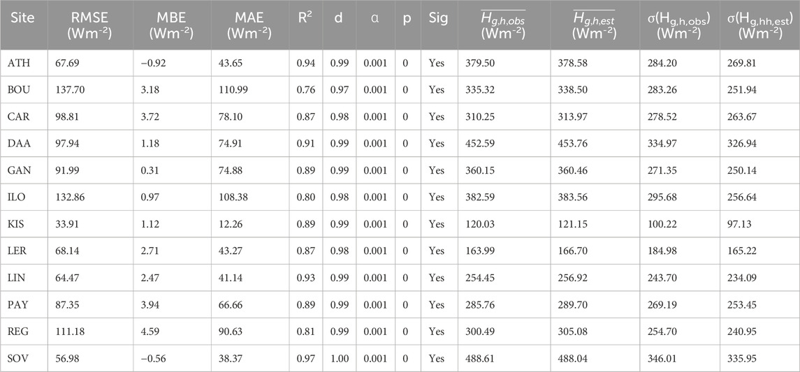
Table 2. Statistical estimators per site for the evaluation of the CPR-estimated hourly Hg,h values with the observed ones by using linear regression analysis. All regression analyses were derived at the 99.9% CI (α = 0.001). The overbars and σ() denote the annual average and standard deviation, respectively, while the subscripts obs and est refer to the corresponding observed and estimated values. All numbers have been rounded to the second decimal digit except for p, which is integer.
The CPR models (Table 2) at 8 (namely BOU, CAR, GAN, ILO, KIS, LER, PAY, and REG) out of the 12 sites provide R2 < 0.90; the lowest accuracy is shown at the BOU site (R2 = 0.76). Nevertheless, this is not the only criterion to decide about the CPR’s performance. These 8 models (especially BOU, ILO, and REG) show higher values of RMSE and MAE than the remaining 4 sites (i.e., ATH, DAA, LIN, SOV), while the MBE values of the 8 sites are not that greater than those for the remaining 4 sites. The higher RMSE values of the 8 sites conclude that there is a great dispersion of the residuals (estimated hourly values − observed hourly values) and, therefore, the observed data is not tightly deployed around the predicted values. Along the same line, the great MAE values of the same sites imply that the estimated values are not so close to the observed ones. On the contrary, their MBE values do not follow the high values of the RMSE and MAE; this means that the models at these sites overestimate the actual data so many times as they underestimate them; the result is that the overestimations are cancelled out by the underestimations. Nevertheless, for all the 12 stations d ≈ 1, which indicates perfect agreement between the estimated and the observed hourly values; this may seem awkward in relation to the previous statistical indicators, but it can be taken as a close follow-up of the estimated to the observed hourly values, i.e., very similar patterns in the solar radiation variability. In conclusion, the CPR methodology seems to be quite successful for the ATH, DAA, LIN, and SOV sites at the hourly level and less successful, but acceptable, at the other 8 locations. This is a differentiation to the conclusion drawn by Yao et al. (2015) who found that the CPR model is accurate for just one location in China (i.e., Jiading). To prove the truth of the above statistical results, Figure 2 shows the variation of the estimated versus the observed hourly Hg,h values for all the sites. The linear regression equations for the scatter plots in Figure 2 are given in Table 3. These findings corroborate the overall significance of the regression models. In general, the CPR models seem to have a good performance at 11 sites and an inferior one for 1 site (BOU).
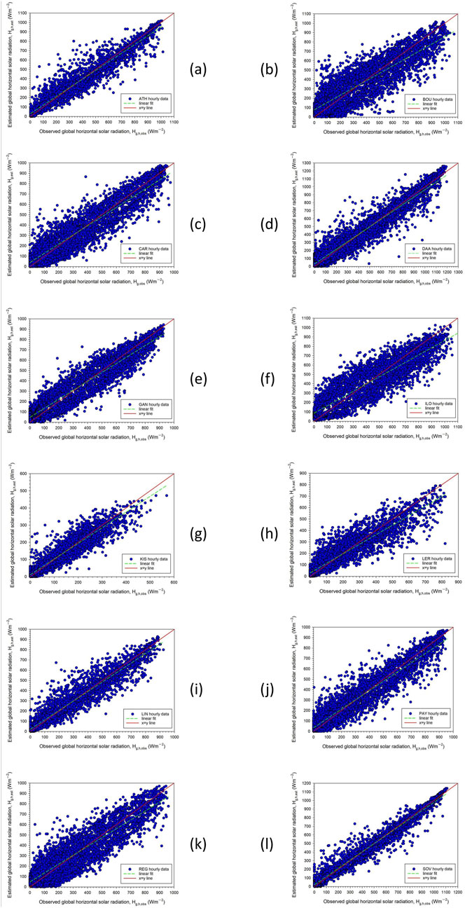
Figure 2. Scatter plots of the hourly mean Hg,h,est estimated values from the CPR model versus the Hg,h,obs observed ones for the 12 sites (panels (A-L), respectively) during the year for each of them. The solid red lines indicate the 1:1 lines and the green dotted ones the linear fits to the Hg,h,est - Hg,h,obs data pairs. All the linear regressions are significant at the 99.9% CI.
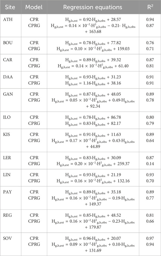
Table 3. Regression equations for the observed versus the estimated solar radiation hourly data at all the 12 sites at the 99.9% CI by using the CPR-model expressions (1)–(5) and the CPRG-model ones (6)–(12); the corresponding R2 values have been taken from Tables 2, 4, respectively. All numbers have been rounded to the second decimal digit.
The CPRG models (Table 4) at only 2 (namely DAA, and SOV) out of the 12 sites provide R2 > 0.90. Though a non-linear regression has been applied to the estimated-observed hourly pairs, this does not prove so successful for the majority of the sites as in the case of the CPR model. The values of the RMSE, MBE, MAE, and R2 statistical indices are now worse than those for the same sites and the CPR models. Nevertheless, d ≈ 1 at all the sites (except for LER with d = 0.53), a result that is interpreted in the same way as for the CPR models. The lowest accuracy is shown at the LER site (R2 = 0.14, Table 3). In conclusion, the CPRG methodology seems to be less successful for all the sites at the hourly level. This is again a contradiction to the conclusion drawn by Yao et al. (2015) who found that the CPRG model is quite accurate for Jiading, China.
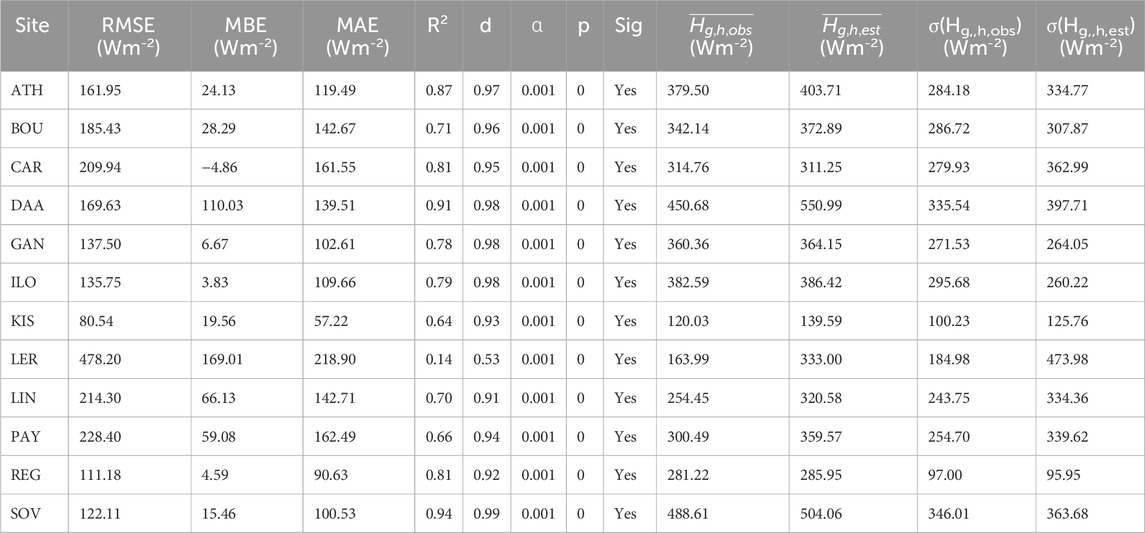
Table 4. Statistical estimators per site for the evaluation of the CPRG-estimated hourly Hg,h values with the observed ones by using non-linear regression analysis. All regression analyses were derived at the 99.9% (α = 0.001) CI. The overbars and σ() denote the annual average and standard deviation, respectively, while the subscripts obs and est refer to the corresponding observed and estimated values. All numbers have been rounded to the second decimal digit except for p, which is integer.
To provide a visual inspection of the statistical results, Figure 3 shows the variation of the estimated versus the observed hourly Hg,h values. The linear regression equations (CPR models) for the scatter plots of Figure 2 are given in Table 3, and the non-linear regression expressions (CPRG models) of Figure 3 in Table 3. One should note that in many sites the quadratic expressions for the CPRG models miss some coefficients; this comes from the regression analysis, which revealed their p values to be greater than 0.001, thereby non-significant coefficients; nevertheless, after removing these coefficients, the regression expressions satisfy the significance test. In general, the CPRG models seem not to have as a good performance as the CPR models at all the sites at the hourly level.
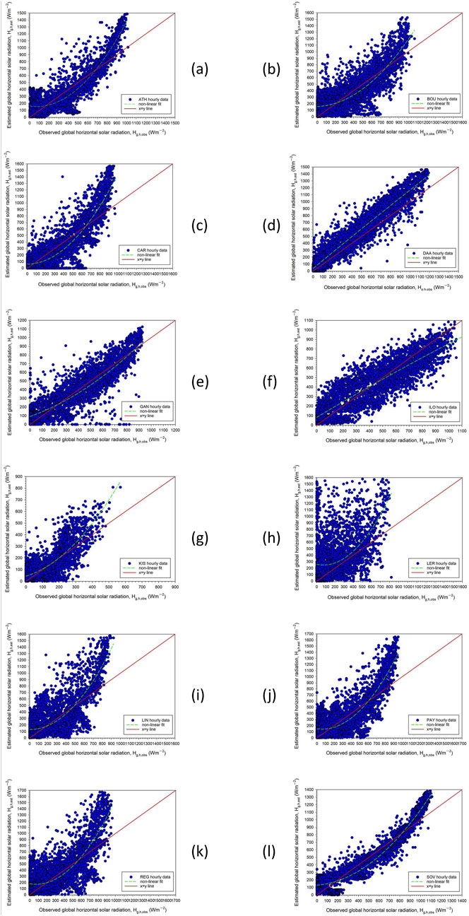
Figure 3. Scatter plots of the hourly mean Hg,h,est estimated values from the CPRG model versus the Hg,h,obs observed ones for the 12 sites (panels (A-L), respectively) during the year for each of them. The solid red lines indicate the 1:1 lines and the green dotted ones the linear fits to the Hg,h,est - Hg,h,obs data pairs. All the non-linear regressions are significant at the 99.9% CI.
3.2 Evaluation of the CPR and CPRG models at the daily scale
After examining the efficiency of the CPR and CPRG models at the hourly level, it would be interesting to see whether the models can reproduce the daily Hg,d values. To do this, the observed and estimated hourly mean Hg,h values at all the sites were converted into daily mean ones. Figure 4 provides the results for the CPG and CPRG models together for space saving. The statistical indicators used in Section 3.1 have been omitted here, because the graphs in Figure 4 speak for themselves. One can easily conclude that the CPR models perform almost ideally, since the estimated-observed daily pairs coincide with the 1:1 line and their R2 values are practically equal to 1. The CPRG models fail to reproduce the daily solar radiation values, especially in the case of the BOU and LER sites.
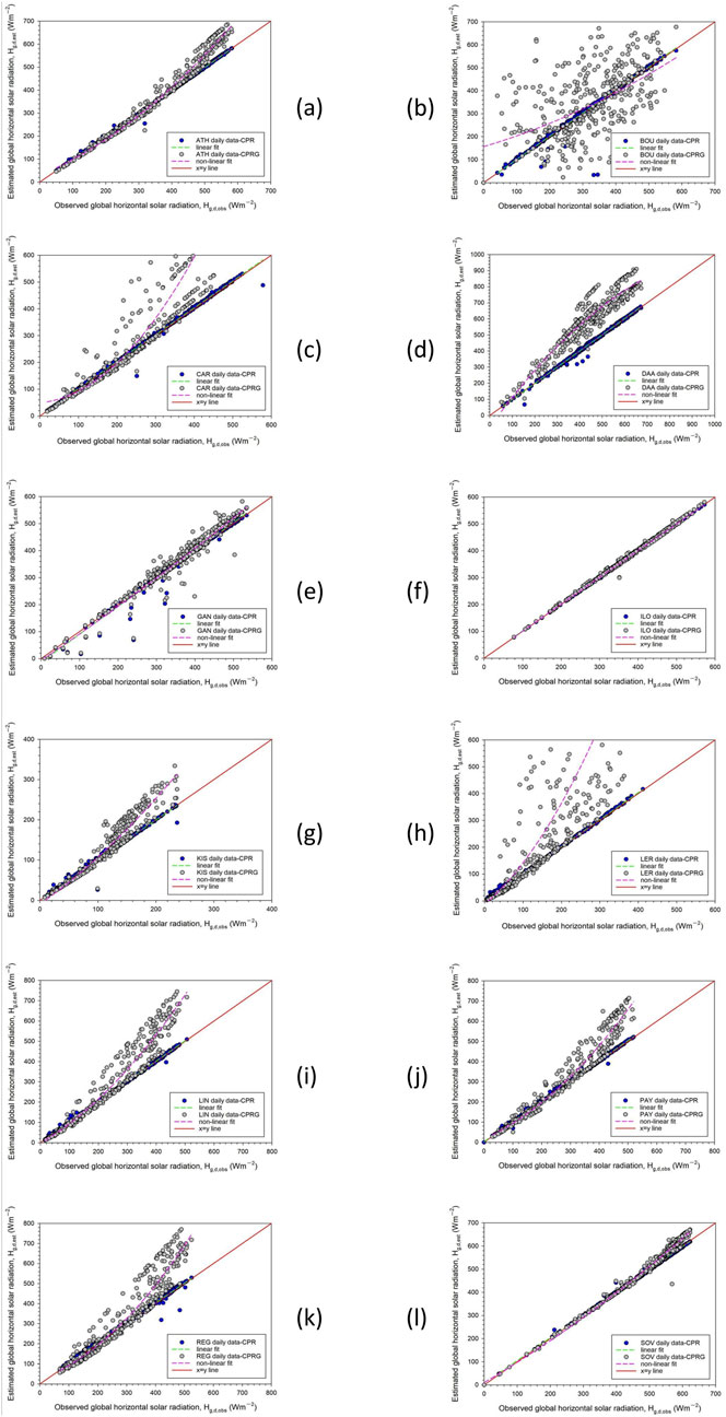
Figure 4. Scatter plots of the daily mean Hg,d,est estimated values from the CPR and CPRG models versus the Hg,d,obs observed ones for the 12 sites (panels (A-L), respectively) during the year for each of them. The solid red lines indicate the 1:1 lines, the green dotted ones the linear fits to the Hg,d,est - Hg,d,obs data pairs for the CPR and the pink dotted lines for the CPRG model. The R2 values are as follows. CPR model: ATH (1.00), BOU (0.95), CAR (1.00), DAA (1.00), GAN (0.98), ILO (1.00), KIS (0.99), LER (1.00), LIN (1.00), PAY (1.00), REG (0.99), and SOV (0.99). CPRG model: ATH (0.98), BOU (0.29), CAR (0.88), DAA (0.89), GAN (0.92), ILO (1.00), KIS (0.93), LER (0.59), LIN (0.94), PAY (0.96), REG (0.92), and SOV (0.99). All the linear and non-linear regressions are significant at the 99.9% CI.
3.3 Evaluation of the CPR and CPRG models at the monthly scale
The last evaluation of the selected DGSRD models concerns the monthly level. As in Section 3.2, the hourly mean Hg,h values at all the sites were converted into monthly mean ones in both models. The results are shown graphically in Figure 5 for the CPR and CPRG models together for space saving. It is evident to conclude that the CPR models are superior to the CPRG ones, because they lie along the 1:1 lines at all the sites.
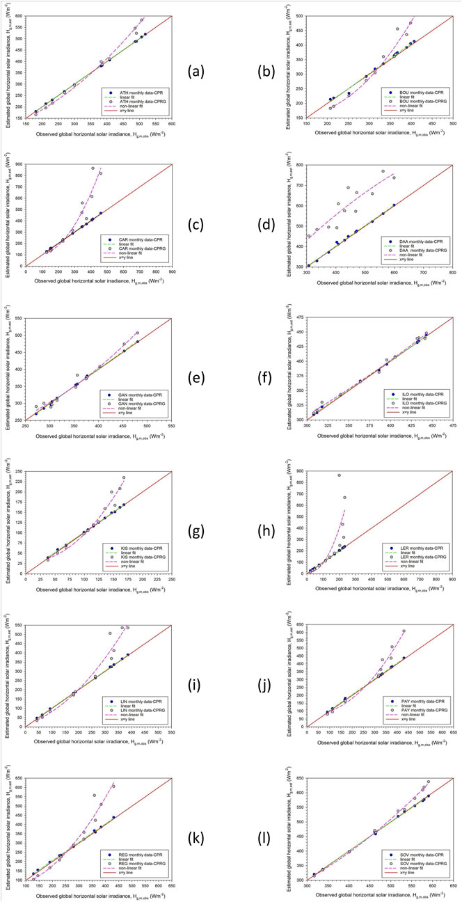
Figure 5. Scatter plots of the monthly mean Hg,m,est estimated values from the CPR and CPRG models versus the Hg,m,obs observed ones for the 12 sites (panels (A-L), respectively) during the year for each of them. The solid red lines indicate the 1:1 lines, the green dotted ones the linear fits to the Hg,m,est - Hg,m,obs data pairs for the CPR and the pink dotted lines for the CPRG model. The R2 values are as follows. CPR model: ATH (1.00), BOU (0.99), CAR (1.00), DAA (1.00), GAN (1.00), ILO (1.00), KIS (1.00), LER (1.00), LIN (1.00), PAY (1.00), REG (1.00), and SOV (1.00). CPRG model: ATH (0.99), BOU (0.96), CAR (0.92), DAA (0.81), GAN (0.98), ILO (0.99), KIS (0.97), LER (0.61), LIN (0.96), PAY (0.98), REG (0.95), and SOV (1.00). All the linear and non-linear regressions are significant at the 99.9% CI.
3.4 Error analysis
This Section is devoted to the errors derived from the modelled data in relation to the observed one. The statistics used here refer to the PE and SE described in Section 2.2.4. Now,
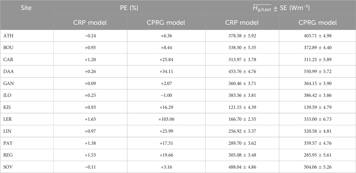
Table 5. Statistical indices of percent error (PE) and standard error (SE) for the error analysis of both DGSRD models at the 12 sites. The SE values were combined with the solar radiation estimated averages at each site for both models; the averages of Hg,h,est have been taken from Tables 2, 4 for the CPR and CPRG models, respectively.
The SE was calculated by taking into account the entire Hg,h,est time series at each site. The SE values were found to lie in the range [1.81, 7.30] for the CPR and in the range [1.19, 6.31] for the CPRG model. It is noticed that the SE values are contained in comparable ranges for both models; this is quite reasonable as this statistic refers to the representativeness of the Hg,h,est time series to another repeated estimations for the same site and model. In other words, the mean value of any future Hg,h,est data set will have a 68% probability to lie in the range
To find the propagation error in the Hg,h,est data for each site and model, the error in the mean value was considered as follows. For each site and model the annual Hg,h,est mean was taken into account from Tables 2, 4. New averages A and B were then derived as
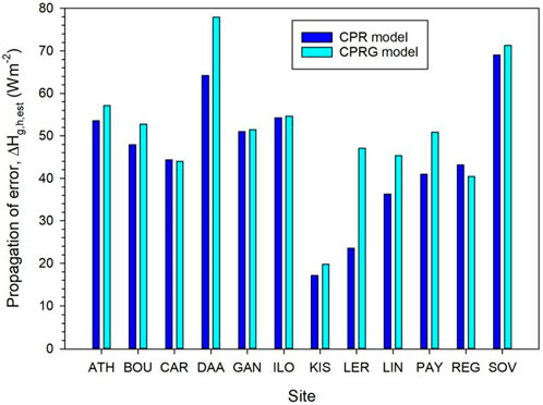
Figure 6. Propagation error, ΔHg,h,est (Wm-2), for both DGSRD models at the 12 sites.
The possible source of extra errors in the CPRG models in comparison with that for the CPR ones may be the non-linear factor fc introduced in the CPRG formulation (see Equation 7). Indeed, if fc is taken equal to 1 for a moment, the CPRG expression coincides with the CPR one. Therefore, a probable improvement for the CPRG model’s performance would be the re-definition or modification of the fc factor.
3.5 Coefficient of correction
In Sections 3.1–3.3 the superiority of the CPR model to the CPRG one was shown. This fact comes from the linearity (along the 1:1 line) of the former and the quadratic behaviour (away from the 1:1 line) of the latter model. Therefore, the present Section deals with the CPR model only.
At this stage, a question may be raised about how to improve further the performance of the CPR model universally. For this reason, the ratios of the monthly averages of Hg,m,obs to the Hg,m,est values were considered for each site. These monthly ratios, named coefficients of correction (CoC), are shown in Figure 7 for all the 12 sites. It is seen that almost all CoC curves fall within the monthly standard deviations except for the BOU and LER sites, which were found in the previous sections not to perform equally well to those of the other 10 sites; indeed, the CoC values of January, November and December for the BOU and LER sites fall outside of the standard deviation limits in these 3 months. Nevertheless, this may not mean a catastrophe, and, therefore, the universal CoCs can be adopted as are.
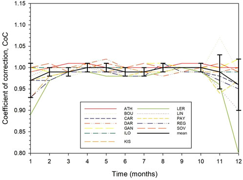
Figure 7. Intra-annual variation of the monthly mean CoC values calculated via the CPR model at all the 12 sites. The solid black line represents the monthly average CoC values and the vertical black bars its standard deviations around the mean.
The CoC values for all the sites were afterwards used in three ways: (i) by multiplying the estimated hourly Hg,h,est values by the annual average CoC = 0.99 calculated from all sites, (ii) by multiplying the estimated hourly Hg,h,est values by the particular monthly averages of CoC (0.97, 0.99, 0.99, 1, 1, 0.99, 0.99, 1, 1, 1, 0.99, 0.96, respectively for January to December) calculated from all sites, and (iii) by multiplying the estimated hourly Hg,h,est values by using the individual monthly averages of CoC for each site. New Hg,h,est values were then derived. The outcome of this process is presented in Figure 8, which shows the annual mean Hg,a (subscript a implies annual) values for the observed, the before-correction-estimated and the after-corrections-estimated values.
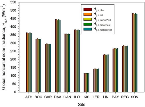
Figure 8. Annual mean values of Hg,a (a = annual) for the observed (obs), estimated (est), estimated corrected with an annual CoC (aaCoC*est), an individual monthly average CoC (mCoC*est), and an overall monthly average CoC (maCoC*est).
The differences in the annual means upon the various estimated values at the sites in comparing them to the observed values are seen to be almost negligible (see Figure 8). To quantify these differences, Table 6 shows them in both Wm-2 and in %. The highest precision in the estimated values is provided by the application of the individual monthly mean CoC values for each site. This gives estimated values equal to the observed ones (column 4, Table 6). Nevertheless, the calculation of the monthly CoC values for every site becomes a tedious work and, in many aspects, not so wise. An acceptable accuracy is given by the application of an annual universal value of CoC = 0.99 (column 3, Table 6), which gives very comparable results to the application of monthly mean universal CoC values (column 5, Table 6). This last conclusion is considered acceptable and may be used worldwide.
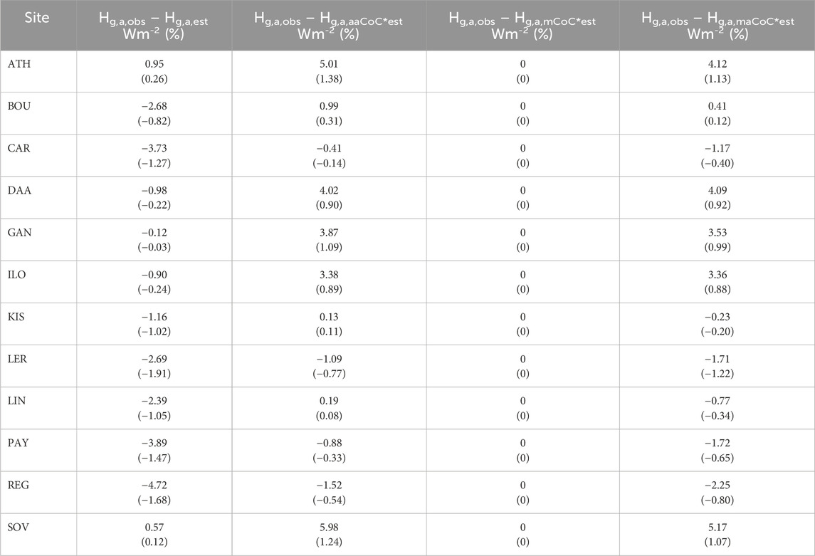
Table 6. Annual differences in Wm-2 and % between the Hg,a,obs values and the Hg,a,est, Hg,a,aaCoC*est, Hg,a,mCoC*est and Hg,a,maCoC*est ones. All numbers have been rounded to the second decimal digit.
A last issue concerning the variation of the annual mean and standard deviation values of CoC for all the sites as function of the absolute geographical latitude (meaning that the − southern latitude of DAA becomes positive) are shown in Figures 9, 10, respectively. Non-linear fits to the data points in both plots have been introduced. There is, though, a guess that these fits may become flat in the range 0o < |φ| < 23.5o if more sites are added in this zone. This conclusion is in line with a similar recent finding by Kambezidis et al. (2023) for the correction factor (CF), as function of |φ|; the CF has been defined as the ratio of energy received on an inclined plane by taking into account a near-real ground albedo to that under the constant albedo value of 0.2. It is interesting to note that the zone [−23.5o, +23.5o] lies between the Tropic of Capricorn in the southern hemisphere and the Tropic of Cancer in the northern one. The average CoCs in Figure 9 show a decline after the latitude of |φ| > 23.5o; this can be interpreted as a lesser need to correct the CPR-estimated solar radiation values as an increase in |φ| is associated with fewer clear-sky (CS) days and, therefore, lower CS solar radiation levels. On the contrary, the decrease in CS events with an increase in |φ| results in a higher dispersion of the CS and non-CS events, thereby increasing σ(CoC).
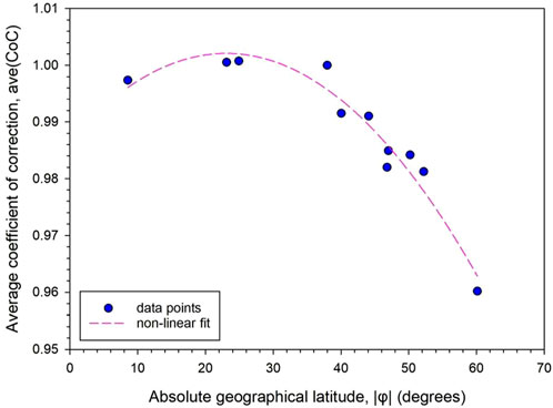
Figure 9. Annual mean CoC values, ave(CoC), as function of the absolute geographical latitude, |φ|, of the 12 sites.

Figure 10. Annual standard deviation values of CoC, σ(CoC), as function of the absolute geographical latitude, |φ|, of the 12 sites.
4 Discussion
The performance of two DGRSD models that can generate hourly global horizontal solar radiation (Hg,h) values at a site from recorded daily values under all-sky conditions was thoroughly investigated in this work. The CPR (Collares-Pereira and Rabl) and the CPRG (Collares-Pereira, Rabl and Gueymard) were the two models chosen. Twelve global locations were chosen for this purpose in order to demonstrate whether or not both models are applicable everywhere. Since the goal was to demonstrate the effectiveness of the models rather than to provide climatological results, specific years for each place were utilised rather than a range of years.
Several statistical indices, including RMSE, MBE, MAE, R2, and d, at the 99.9% CI, were employed to assess the models’ performance. The hourly Hg,h ratios were calculated by multiplying the hourly rCPR and rCPRG ratios (Equations 1, 6, respectively) by the daily Hg,d values.
The observed and calculated hourly Hg,h values were contrasted. The CPR models produced R2 < 0.90 for 8 of the 12 sites (BOU, CAR, GAN, ILO, KIS, LER, PAY, and REG). However, while the MBEs of the 8 sites were not significantly higher than those of the other 4, the RMSE and MAE values of the aforementioned 8 models (particularly BOU, ILO, and REG) were higher. The BOU site had the lowest accuracy (R2 = 0.76). However, the result of d ≈ 1 for every site showed perfect agreement between the estimated and observed values. In summary, the CPR methodology appears to be quite effective for the ATH, DAA, LIN, and SOV locations at the hourly level. Overall, the CPR models appear to perform well across all locations, with BOU showing a lower performance. Out of the 12 sites, only 2 (DAA and REG) have CPRG models that yielded R2 > 0.90. These two sites’ RMSE, MBE, MAE, and R2 statistical index values were found lower than those of the CPR models and the identical sites. However, d ≈ 1 at every site, which is comparable to the CPR models’ outcome. The LER site had the lowest accuracy (R2 = 0.14). In summary, the CPR modelling appears to be more effective than the CPRG methodology at the hourly level for all sites.
At every site and in both models, the hourly Hg,h values that were observed and calculated were transformed into daily Hg,d values. For the 12 locations and both models, twelve scatter plots were created for the Hg,m,est–Hg,m,obs pairs. For the CPR and CPRG models, linear and quadratic fits were obtained, respectively. Only the data pairs pertaining to CPR were discovered to be along the 1:1 line, despite the fact that both regression fits had extremely high R2 values. In summary, it was discovered that the CPR models performed nearly flawlessly; however, the CPRG models were unable to replicate the daily values, particularly for the BOU and LER sites.
The monthly level was the focus of the most recent assessment of the chosen DGSRD models. For both models, the hourly mean Hg,h data at each site was transformed into monthly mean Hg,m values. Regression fits were derived to the Hg,m,est – Hg,m,obs data pairs, and scatter plots were created similarly to the daily-scale case. Finding that the data at every site falls along the 1:1 lines confirmed once more that the CPR model outperforms the CPRG one.
The following was shown by an error analysis of the Hg,h,est hourly values at each site and in both DGSRD models. While the PE for the CPRG model was found to be higher, indicating a poorer performance compared to the CPR model, the percent error for the CPR model fell within the acceptable range of ±5% about the individual annual Hg,h,est average. The standard error analysis of the Hg,h,est data set revealed that, for the same location and model, the mean value of any subsequent Hg,h,est data set will probably fall within the range
The coefficient of correction (CoC) was defined as the ratio between the observed to the estimated solar radiation values. This was carried out to look into the potential for further enhancing the CPR models’ performance. CoCs were determined using 3 methods: (i) an overall annual average for all sites, (ii) monthly averages for each site, and (iii) overall monthly averages for all sites. For the 3 CoC methods, the differences between the yearly mean values of Hg,a,obs and Hg,a,est were computed in both Wm-2 and %. The differences were found negligible, thus concluding that the overall annual average of CoC = 0.99 can be used universally to bring the hourly CPR-derived values closer to the observed ones. In practical terms, the universal CoC value is useful in the transformation of hourly, daily or monthly global horizontal solar radiation data that can be obtained via satellite observations, solar modelling or data re-analysis at regions that do not have access to these types of measurements. Naturally, even though this CoC value is universal, it could change if other sites are added in a future study.
Ultimately, the current study showed that the CPR model is highly practical and applicable globally. However, in order to confirm its universality, the methodology created in this work should be applied to more locations worldwide in future research. Particularly, if new sites are chosen in the zone 0o < |φ| < 30o, this could improve the effectiveness of the CPR models and validate the conclusion made in Section 3.5 with a potential explanation of the significance of this occurrence using machine-learning techniques.
Data availability statement
Publicly available datasets were analysed in this study. This data can be found at: Baseline Solar Radiation Network (https://bsrn.awi.de/data/data-retrieval-via-pangaea/) and National Observatory of Athens (https://www.iersd.noa.gr/en/services/parochi-klimatikon-dedomenon/, upon request).
Author contributions
HDK: Conceptualisation, Data curation, Methodology, Validation, Visualisation, Writing–original draft, Writing–review and editing.
Funding
The author declares that no financial support was received for the research, authorship, and/or publication of this article.
Acknowledgments
The author is especially grateful to the following scientists: (i) S. Wacker (LIN) and A. Aculinin (KIS) for providing formulated data from their BSRN stations for years 2018 and 2020, respectively; (ii) A. Driemel (World Radiation Monitoring Centre) for providing access to the PANGAEA website (https://bsrn.awi.de/data-retrieval-via-pangaea, accessed on 1 July 2021) and downloading data from 10 BSRN stations. Data from the ATH station has been possessed by the author as member of the Institute where the station belongs to and as the responsible scientist for the station’s smooth operation until 2014. Also acknowledged are the following scientists who are/were responsible for their BSRN stations used in this study: S. Morris BOU; J.F. Morel CAR; J. Botai DAA; P. Kumar GAN; T.O. Aro ILO; G. Hodgetts LER; L. Vuilleumier PAY; D. Halliwell REG; M. Olefs SON; N. Al-Abbadi SOV.
Conflict of interest
The author declares that the research was conducted in the absence of any commercial or financial relationships that could be construed as a potential conflict of interest.
Generative AI statement
The author(s) declare that no Generative AI was used in the creation of this manuscript.
Publisher’s note
All claims expressed in this article are solely those of the authors and do not necessarily represent those of their affiliated organizations, or those of the publisher, the editors and the reviewers. Any product that may be evaluated in this article, or claim that may be made by its manufacturer, is not guaranteed or endorsed by the publisher.
References
Baig, A., Akhter, P., and Mufti, A. (1991). A novel approach to estimate the clear day global radiation. Renew. Energy 1 (1), 119–123. doi:10.1016/0960-1481(91)90112-3
Bojinski, S., Verstraete, M., Peterson, T. C., Richter, C., Simmons, A., and Zemp, M. (2014). The concept of essential climate variables in support of climate research, applications, and policy. Bull. Am. Meteorological Soc. 95 (9), 1431–1443. doi:10.1175/BAMS-D-13-00047.1
Boscaini, R., Robaina, A. D., Peiter, M. X., Bruning, J., Rodrigues, S. A., da Silva, J. G., et al. (2020). Performance of solar radiation models for obtaining reference evapotranspiration to Santa Maria-RS, Brazil. Rev. Bras. Ciencias Agrar. 15 (1), 1–8. doi:10.5039/AGRARIA.V15I1A7661
Christie, M. A., Glimm, J., Grove, J. W., Higdon, D. M., Sharp, D. H., and Wood-Schultz, M. M. (2005). Error analysis and simulations of complex phenomena. Los Alamos Sci. 29, 6–25.
Collares-Pereira, M., and Rabl, A. (1979). The average distribution of solar radiation-correlations between diffuse and hemispherical and between daily and hourly insolation values. Sol. Energy 22 (2), 155–164. doi:10.1016/0038-092X(79)90100-2
Driemel, A., Augustine, J., Behrens, K., Colle, S., Cox, C., Cuevas-Agulló, E., et al. (2018). Baseline surface radiation network (BSRN): structure and data description (1992–2017). Earth Syst. Sci. Data 10 (3), 1491–1501. doi:10.5194/essd-10-1491-2018
El shazly, S. M. (1996). Estimation of hourly and daily global solar radiation at clear days using an approach based on modified version of Gaussian distribution. Adv. Atmos. Sci. 13, 349–358. doi:10.1007/bf02656852
Garg, H. P., and Garg, S. N. (1987). Improved correlation of daily and hourly diffuse radiation with global radiation for Indian stations. Sol. Wind Technol. 4 (2), 113–126. doi:10.1016/0741-983X(87)90037-3
Giesen, R. H., van den Broeke, M. R., Oerlemans, J., and Andreassen, L. M. (2008). Surface energy balance in the ablation zone of Midtdalsbreen, a glacier in southern Norway: interannual variability and the effect of clouds. J. Geophys. Res. 113 (D21), D21111. doi:10.1029/2008JD010390
Gueymard, C. (1986). Mean daily averages of beam radiation received by tilted surfaces as affected by the atmosphere. Sol. Energy 37 (4), 261–267. doi:10.1016/0038-092X(86)90043-5
Gueymard, C. (2000). Prediction and performance assessment of mean hourly global radiation. Sol. Energy 68 (3), 285–303. doi:10.1016/S0038-092X(99)00070-5
Jain, P. C. (1984). Comparison of techniques for the estimation of daily global irradiation and a new technique for the estimation of hourly global irradiation. Sol. Wind Technol. 1 (2), 123–134. doi:10.1016/0741-983X(84)90014-6
Jain, P. C. (1988). Estimation of monthly average hourly global and diffuse irradiation. Sol. Wind Technol. 5 (1), 7–14. doi:10.1016/0741-983X(88)90085-9
Kambezidis, H. D. (2021). The solar radiation climate of Greece. Climate 9 (12), 183. doi:10.3390/cli9120183
Kambezidis, H. D. (2022). “The solar resource,”Compr. Renew. Energy Editor T. M. Letcher, 26–117. doi:10.1016/B978-0-12-819727-1.00002-9
Kambezidis, H. D., Kavadias, K. A., and Farahat, A. M. (2024). Solar energy received on flat-plate collectors fixed on 2-Axis trackers: effect of ground albedo and clouds. Energies 17, 3721–3727. doi:10.3390/en17153721
Kambezidis, H. D., Mimidis, K., and Kavadias, K. A. (2022). Correction of the solar azimuth discontinuity at sunrise and sunset. Sun Geosph. 15 (1), 39–44. doi:10.31401/SunGeo.2022.01.04
Kambezidis, H. D., Mimidis, K., and Kavadias, K. A. (2023). The solar energy potential of Greece for flat-plate solar panels mounted on double-Axis systems. Energies 16 (13), 5067. doi:10.3390/en16135067
Kambezidis, H. D., and Tsangrassoulis, A. E. (1993). Solar position and right ascension. Sol. Energy 50 (5), 415–416. doi:10.1016/0038-092X(93)90062-S
Kambezidis, H. D. D., and Papanikolaou, N. S. S. (1990). Solar position and atmospheric refraction. Sol. Energy 44 (3), 143–144. doi:10.1016/0038-092X(90)90076-O
Khatib, T., Mohamed, A., and Sopian, K. (2012). A review of solar energy modeling techniques. Renew. Sustain. Energy Rev. 16 (5), 2864–2869. doi:10.1016/j.rser.2012.01.064
Larsen, K. S., Ibrom, A., Beier, C., Jonasson, S., and Michelsen, A. (2007). Ecosystem respiration depends strongly on photosynthesis in a temperate heath. Biogeochemistry 85 (2), 201–213. doi:10.1007/s10533-007-9129-8
Liu, B. Y. H., and Jordan, R. C. (1960). The interrelationship and characteristic distribution of direct, diffuse and total solar radiation. Sol. Energy 4 (3), 1–19. doi:10.1016/0038-092X(60)90062-1
Newell, T. A. (1983). Simple models for hourly to daily radiation ratio correlations. Sol. Energy 31 (3), 339–342. doi:10.1016/0038-092X(83)90024-5
Nwokolo, S. C., Amadi, S. O., Obiwulu, A. U., Ogbulezie, J. C., and Eyibio, E. E. (2022). Prediction of global solar radiation potential for sustainable and cleaner energy generation using improved Angstrom-Prescott and Gumbel probabilistic models. Clean. Eng. Technol. 6 (May 2021), 100416. doi:10.1016/j.clet.2022.100416
Taylor, J. R. (1982). An introduction to error analysis. 2nd edition, Vol. 101. Sausalito, CA: University Science Books.
Walraven, R. (1978). Calculating the position of the sun. Sol. Energy 20 (5), 393–397. doi:10.1016/0038-092X(78)90155-X
Whillier, A. (1956). The determination of hourly values of total solar radiation from daily summations. Arch. Für Meteorol. Geophys. Und Bioklimatol. Ser. B 7 (2), 197–204. doi:10.1007/BF02243322
Yao, W., Li, Z., Xiu, T., Lu, Y., and Li, X. (2015). New decomposition models to estimate hourly global solar radiation from the daily value. Sol. Energy 120, 87–99. doi:10.1016/j.solener.2015.05.038
Nomenclature
Abbreviations
AI artificial intelligence
amsl above mean sea level
ANN artificial neural network
ASNOA actinometric station of the National Observatory of Athens
BSRN baseline surface radiation network
CI confidence interval
CoC coefficient of correction
CPR model Collares-Pereira and Rabl model
CPRG model Collares-Pereira, Rabl and Gueymard model
CS clear skies
DGSRD model daily global solar radiation decomposition model
LST local standard time
MAE mean-absolute error
MBE mean-bias error
PE percent error
RMSE root mean-square error
SE standard error
UTC universal time coordinated
Symbology
γ solar altitude (degrees)
δ solar declination (degrees)
λ geographical longitude (degrees)
σ standard deviation
φ geographical latitude (degrees)
ψ solar azimuth (degrees)
ω solar hour angle (degrees)
d index of agreement
Hg global horizontal solar irradiance (Wm-2)
R2 coefficient of determination
N number of data points
z altitude (m)
Keywords: solar radiation, decomposition models, hourly values, daily values, monthly values, universal applicability
Citation: Kambezidis HD (2025) An in-depth analysis of two common methodologies used to derive hourly solar radiation values from daily ones: pros and cons. Front. Environ. Sci. 13:1528355. doi: 10.3389/fenvs.2025.1528355
Received: 14 November 2024; Accepted: 08 January 2025;
Published: 29 January 2025.
Edited by:
Georgios E. Arnaoutakis, Hellenic Mediterranean University, GreeceReviewed by:
Nikolaos Savvakis, Technical University of Crete, GreeceItyona Amber, Robert Gordon University, United Kingdom
Copyright © 2025 Kambezidis. This is an open-access article distributed under the terms of the Creative Commons Attribution License (CC BY). The use, distribution or reproduction in other forums is permitted, provided the original author(s) and the copyright owner(s) are credited and that the original publication in this journal is cited, in accordance with accepted academic practice. No use, distribution or reproduction is permitted which does not comply with these terms.
*Correspondence: Harry D. Kambezidis, aGFycnlAbm9hLmdy, aGFycnlAdW5pd2EuZ3I=