Short-term PM2.5 forecasting using a unique ensemble technique for proactive environmental management initiatives

Particulate matter with a diameter of 2.5 microns or less (${\text{PM}}_{2.5}$) is a significant type of air pollution that affects human health due to its ability to persist in the atmosphere and penetrate the respiratory system. Accurate forecasting of particulate matter is crucial for the healthcare sector of any country. To achieve this, in the current work, a new time series ensemble approach is proposed based on various linear (autoregressive, simple exponential smoothing, autoregressive moving average, and theta) and nonlinear (nonparametric autoregressive and neural network autoregressive) models. Three ensemble models are also developed, each employing distinct weighting strategies: equal distribution of weight among all single models (ESME), weight assignment based on training average accuracy errors (ESMT), and weight assignment based on validation mean accuracy measures (ESMV). This technique was applied to daily ${\text{PM}}_{2.5}$ concentration data from 1 January 2019, to 31 May 2023, in Pakistan’s main cities, including Lahore, Karachi, Peshawar, and Islamabad, to forecast short-term ${\text{PM}}_{2.5}$ concentrations. When compared to other models, the best ensemble model (ESMV) demonstrated mean errors ranging from 3.60% to 25.79% in Islamabad, 0.81%–13.52% in Lahore, 1.08%–7.06% in Karachi, and 1.09%–12.11% in Peshawar. These results indicate that the proposed ensemble approach is more efficient and accurate for short-term ${\text{PM}}_{2.5}$ forecasting than existing models. Furthermore, using the best ensemble model, a forecast was made for the next 15 days (June 1 to 15 June 2023). The forecast showed that in Lahore, the highest ${\text{PM}}_{2.5}$ value (236.00 $\mu g/m^3$) was observed on 8 June 2023. Other days also displayed higher and poor air quality throughout the 15 days. Conversely, Karachi experienced moderate ${\text{PM}}_{2.5}$ concentration levels between 50 $\mu g/m^3$ and 80 $\mu g/m^3$. In Peshawar, the ${\text{PM}}_{2.5}$ concentration levels were consistently unhealthy, with the highest peak (153.00 $\mu g/m^3$) observed on 9 June 2023. This forecasting experience can assist environmental monitoring organizations in implementing cost-effective planning to minimize air pollution.

1 Introduction

Maintaining a healthy atmosphere is vital for both humans and other living creatures. Air quality refers to the absence of harmful pollutants in the air. However, there are several deadly and fatal contaminants in the air nowadays, including ${\text{PM}}_{2.5}$, nitrogen dioxides (${\text{NO}}_2$), carbon monoxides (CO), sulfur dioxides (${\text{SO}}_2$), ozone (${\text{O}}_3$), and ${\text{PM}}_{10}$ are the most hazardous pollutants, and these and several more contaminants cause air pollution (Donahue, 2018; Quispe et al., 2024; Yin et al., 2023; Shang and Luo, 2021). Currently, air pollution is increasing rapidly due to urbanization, industrialization, and overcrowding, and this leads to a significant increase in respiratory problems, premature birth, premature death, and lung disease, which cause death. The World Health Organization estimates that air contamination claims the lives of about ten million people each year. As discussed above, air pollutants contribute significantly to air quality degradation and affect human health and the environment due to increased industrial and human activity and the continuous use of fossil fuels (Manisalidis et al., 2020; Luo et al., 2024; Qiu et al., 2024; Shang et al., 2023). Currently, air pollution is Pakistan’s most significant and alarming challenge, continuously being mentioned by social media and other platforms. This air pollution in Pakistan causes different health-related problems, mainly cardiac and respiratory. Thus, particular actions must be taken to prevent or reduce air pollution (Ullah et al., 2021; Iftikhar et al., 2024c; Du and Wang, 2013; Chen et al., 2024).

In the past, many researchers have developed solutions to this problematic air pollution issue. In this context, many researchers have applied classical regression, time series, machine learning, and hybrid models to find the optimum solution according to the nature of the data (Zhan et al., 2017; Xu et al., 2018; Abdullah et al., 2019; Dutta and Jinsart, 2021). For instance, the work (Geetha and Prasika, 2019) provides an LSTM in addition to two conventional forecasting models for estimating the levels of air pollutants (NO₂, NOx, CO, SO₂, O3, PM2.5, and PM10) in metropolises. The outcomes demonstrated that LSTM outperformed LR and ARIMA. Zaman et al. (2024) attempt intends to create machine learning models that are computationally efficient and simpler than those found in earlier studies. Findings indicated that the RF methodology performed marginally better than the XG-Boost and SVR techniques. In another research work, Zaman et al. (2021) predict $P{M}_{2.5}$ concentrations throughout Malaysia by utilizing satellite-based AOD data to drive machine learning (ML) models such as (RF) and (SVR). Seven models were created for $P{M}_{2.5}$ prediction. The testing analysis shows that the RF framework (R2 = 0.53–0.76) performs somewhat superior to SVR. On the other hand, using the most recent data on diseases and smog degree of severity, this study (Chen et al., 2017) designed an ANN-based model to forecast health hazards associated with smog. The outcomes demonstrated that empirical insights can aid researchers in getting the nonlinear correlations between the health risk the following day and present-day smog observations.

This work (Freeman et al., 2018), a forecast model for ozone levels averaged over 8 hours, was trained using novel deep learning techniques. A new technique for imputation was used to replace missing data and outliers in the collected data set. This method produced computed values based on the time and season closer to the predicted value. (Carbo-Bustinza et al., 2023). Using a comparison of numerous hybrid varieties of time series models, this work extensively studies projecting ozone concentrations. According to the study, the suggested models perform noticeably superior to the standard models that were considered. However, this research (Xie et al., 2021) aims to apply the Hausdorff distance method to huge data to improve future cyclone effect predictions (Rakholia et al., 2023). Analyzed to develop a multi-step-ahead with multi-output type multivariate statistical model (NBEATS) to estimate the air quality with the auxiliary information. The data set was collected from six healthcare air quality centers in Vietnam. To compare the results and efficiency with the existing model, accuracy indices such as MAPE and RMSE were used. The result indicated that the developed (d-BEATS) multi-dimensional co-variate model outperforms the existing models. In the work Bhatti et al. (2021), the researcher conducted a comparative study to estimate the air quality index for Pakistan. They used the SARIMA and factor analysis approaches to achieve this end. The study found that the SARIMA model outperforms others in attaining better estimation accuracy for Pakistan’s air quality index. In another work, Ashraf et al. (2022) conducted an analysis based on the comparative study of machine learning and classical forecasting models to forecast air pollution data. This article uses the metrics, i.e., RMSE, MAE, and MAPE, to compare the classical and traditional models. The study suggested that the machine learning model performed more efficiently than the existing time series methods.

In the same way, Lin et al. (2019) performed an analysis based on machine learning and integrated assimilation data techniques to expand the air quality prediction for the Netherlands. The findings disclosed that the developed approach, which incorporates data-driven machine learning and a physics-based model, significantly improved the air quality forecast statistically. However, Kleine Deters et al. (2017) modeled ${\text{PM}}_{2.5}$ urban pollution (Cotocollao and Belisario) using machine learning techniques. Based on the proposed machine learning model concentrations of ${\text{PM}}_{2.5}$, the classifier accurately predicted ${\text{PM}}_{2.5}$. Moreover, it was also observed that regression highlights better prediction when there are extreme conditions in the climate. This article shows that statistical approaches to machine learning techniques are relevant and significant in modeling ${\text{PM}}_{2.5}$. Also, Borse (2020) highlighted the systematic review based on different statistical and machine learning techniques to forecast air quality. This systematic review concludes that data mining and machine learning approaches are highly used in forecasting and predicting air pollution. In another research, the author in Liu et al. (2020) analyzed the air quality index using machine learning algorithms. In this research work, the authors developed a novel machine-learning model based on the LSTM method and compared it with existing models. The results indicated that the developed model outputs were superior to the existing machine learning models in forecasting ${\text{PM}}_{2.5}$. Garg and Jindal (2021) conducted a comparative study between machine learning and classical time series models to estimate ${\text{PM}}_{2.5}$. The study found that the LSTM model outputs better and superior accuracy than the existing approaches. However, Ameer et al. (2019) conducted a comparative analysis based on advanced regression methods to predict the air quality index of smart cities. This article used RMSE and MAE to evaluate the underlying models. The study found that the random forest model outperformed the existing methods.

On the other hand, Wang et al. (2019) proposed a hybrid model for air quality variables forecasting. This proposed method is a hybridization of the Long Short-Term Memory Neural Network and Gated Recurrent Unit (LSTM and GRU), an enhancement of ordinary LSTM. This work uses the data set of 74 cities in China for a comparative study. The outcomes disclosed that the proposed hybrid model outperformed the existing approaches. In the same way, Ejohwomu et al. (2022) conducted a comprehensive study to model the ${\text{PM}}_{2.5}$ using hybrid machine learning methods. The finding showed that the hybrid machine-learning model outperformed the existing techniques. Also, Bai et al. (2019) for forecasting the hourly ${\text{PM}}_{2.5}$ concentration, an ensemble neural network (E-LSTM) is proposed. The results show that the E-LSTM model, which comprises multiple LSTMs in different modes, outperforms the single LSTM regarding MAPE, RMSE, and correlation. Thus, different authors used various methods and models to find the optimum solution according to the nature of the data.

In contrast to the research mentioned earlier, this study introduces a comparatively simple and easily implemented new time series ensemble technique based on various linear (autoregressive, simple exponential smoothing, autoregressive moving average, and theta) and nonlinear (nonparametric autoregressive and neural network autoregressive) models to accurately and efficiently forecast short-term ${\text{PM}}_{2.5}$ concentration in highly populated cities of Pakistan, including Lahore, Peshawar, Karachi, and Islamabad. Three ensemble models are developed, each using different weighting strategies: equal distribution of weight among all single models (ESME), weight assignment based on training average accuracy errors (ESMT), and weight assignment based on validation mean accuracy measures (ESMV). In this proposed time series ensemble approach, the ${\text{PM}}_{2.5}$ time series is first preprocessed by addressing missing values, stabilizing variance, ensuring normality, considering deterministic features, and addressing stationarity concerns. Then, six single time series and three ensemble models are used to forecast the preprocessed ${\text{PM}}_{2.5}$ concentration time series. Six different accuracy metrics—the Diebold and Mariano tests and the correlation plot—are employed to assess the performance of this novel time series ensemble forecasting approach. The main contribution of this study is evaluating the performance of different single time series models and their proposed three novel ensemble models within the time series forecasting approach. The short-term forecasting performance for a whole year for air pollution (${\text{PM}}_{2.5}$) is evaluated, and the significance analysis of the differences in prediction accuracy is also investigated. To confirm the performance of the proposed time series ensemble technique, six different average accuracy metrics, an equal forecast statistical test, and a graphical assessment are used for comparison. This methodological proposal applies to the environmental management system to mitigate ozone pollution and is aimed at the stakeholders of the national air quality program. Unlike previous studies, which have been conducted from various perspectives globally, this analysis uses ensemble time series modeling and forecasting for short-term ${\text{PM}}_{2.5}$ levels in the Pakistan megacities. Finally, this approach could be extended to other cities in Pakistan and worldwide.

2 The proposed time series ensemble forecasting technique

This section elucidates the proposed time series ensemble technique for short-term (one-day-ahead) ${\text{PM}}_{2.5}$ concentration forecasting in the megacities of Pakistan. In the proposed time series ensemble technique, the ${\text{PM}}_{2.5}$ time series is first preprocessed by missing value, variance stabilization, and stationary concerns. Second, six different single time series models: the autoregressive, the simple exponential smoothing, the autoregressive moving averages, the theta, the nonlinear autoregressive, and the neural network autoregressive, and also three proposed ensemble models anticipate the cleaned ${\text{PM}}_{2.5}$ concentration time series. The details about these steps are in the following subsections.

2.1 Preparation of raw data

This work uses daily ${\text{PM}}_{2.5}$ concentration datasets from four monitoring megacities in Pakistan, Islamabad, Lahore, Karachi, and Peshawar, for five consecutive years: 2019, 2020, 2021, 2022, and 2023, respectively. Before starting modeling and estimating a time series of data, it should make sense to prepare the data. The goal of preprocessing is usually to simplify the modeling of the database. The ${\text{PM}}_{2.5}$ concentration time series case involves missing values, high volatility, a nonconstant mean, a long-run secular trend component, and specific seasonality. To achieve these, we first treated the missing values using the multivariate imputation by chained equations (MICE) method (Van Buuren and Oudshoorn, 2011; Zhou et al., 2023). The MICE is a robust, informative method of dealing with missing data in datasets. The procedure imputes missing data in a dataset through an iterative series of predictive models. In each iteration, each specified variable in the dataset is imputed using the other variables. These iterations should be run until convergence has been met. Second, after getting the free missing values ${\text{PM}}_{2.5}$ concentration time series, we get stabilized variance and standard deviation by taking the natural logarithm of each series. Third, the deterministic characteristics containing a linear long-run trend component and yearly seasonality are removed. To accomplish this, model these deterministic components using the following procedure: Let the time series of the ${\text{PM}}_{2.5}$ concentration series be donated by $log(P_d^k)$; the super subscript k $(k=\mathrm{1,2,3,4})$ shows the city series, while d shows the ${\text{d}}^{th}$ day data point. Thus, the dynamics of the log daily ${\text{PM}}_{2.5}$ concentration times series, log$(P_d^k)$, may be described as:

$log\left(P_d^k\right)={\tau }_d^k+a_d^k+p_d^k(1)$

That is, the log$(P_d^k)$ in Equation 1 is divided into these components: a long-run linear trend component $({\tau }_d^k)$, a yearly seasonality component $(a_d^k)$, and a residual component $(p_d^k)$. The $({\tau }_d^k)$ component is a function of the series $(\mathrm{1,2,3},\dots ,d)$, is estimated by the regression splines method, and dummies capture the annual periodicity: $a_{d,j}^k={\displaystyle \sum _{\text{j}=1}^5}{\zeta }_j{I}_{d,j}$. The variable $I_{d,j}$ is assigned a value of 1 when h refers to the ${\text{i}}^{\text{t}h}$ year and 0 otherwise. The regression coefficients $({\zeta }_j)$ associated with these components are determined using the ordinary least square method. It is worth mentioning that many authors in the literature capture the long-run trend and yearly in a time series using regression splines (Shah et al., 2020; Iftikhar et al., 2023c; Shah et al., 2022; Zhu, 2023; Xu et al., 2022). On the other hand, once the estimated deterministic component (long-run trend and annual periodicity) is obtained, the residual or stochastic component can be derived by using Equation 2:

$p_d^k=log\left(P_d^k\right)-\left({\widehat{\tau }}_d^k+{\widehat{a}}_d^k\right)(2)$

Thus, once the air pollutant (${\text{PM}}_{2.5}$) concentration time series is preprocessed (to address the issue of missing values and its imputation, stabilize the variance and standard deviation, and remove the deterministic properties), the next step is to model the remaining residual $p_d^k$ series; the current work considers six single-time series models and three proposed ensemble models. Hence, all forecasting models are described in the coming subsection.

2.2 Forecasting models

This section briefly overviews the forecasting models and their proposed ensemble models: the autoregressive, the simple exponential smoothing, the autoregressive moving average, the Theta, the nonparametric autoregressive, and the neural network autoregressive models.

2.2.1 The auto-regressive model

A linear autoregressive (AR) model is used to understand the short-term dynamics of $p_d$ by using a linear combination of $p$ past observations. The model can be expressed as:

$p_d=\text{I}+{\beta }_1{p}_1+{\beta }_2{p}_2+\cdots .+{\beta }_p{p}_d+{ϵ}_d(3)$

In Equation 3, $p_i$($i=\mathrm{1,2},\dots ,d$) are observed and past values of ${\text{PM}}_{2.5}$, $\beta$ AR parameters, and ${ϵ}_m$ is the white noise process. In this study, we estimated the parameters using maximum likelihood estimation. After analyzing the series’s auto-correlation function (ACF) and partial auto-correlation function (PACF), we concluded that lags 1, 2, 3, and 7 are significant and, therefore, included in the model (Jenkins and Box, 1976; Box et al., 2015).

2.2.2 The exponential smoothing model

The Exponential Smoothing Model (ESM) is a group of forecasting models that apply exponentially decreasing weights to previous observations. It is a time-series forecasting model that uses a weighted average of past observations to predict the future value of a variable. The ES model assumes that a variable’s future value depends on its past values, with greater emphasis placed on recent values than on older ones. The ESM model can be expressed as follows:

$p_{d+1}=\alpha \cdot p_d+\left(1-\alpha \right)\cdot p_{d-1}(4)$

In the given Equation 4, $p_{d+1}$, $p_d$, and $p_{d-1}$ are the actual values of the ${\text{PM}}_{2.5}$ concentration time series at times d+1, d, and d-1. At the same time, $\alpha$ is the smoothing parameter determining the weight assigned to the most recent observation (Brown, 1956; Holt, 2004).

2.2.3 The autoregressive moving average model

The autoregressive moving average (ARMA) models incorporate lagged values from a time series and factor in error terms passed into the model. This study utilized a model representing the residual series $(p_d)$ as a linear combination of $d$ past observations and a delay error term. The model equation can be expressed as:

$\begin{array}{c}\hfill p_d=u+{\beta }_1{p}_1+{\beta }_2{p}_2+\cdots .+{\beta }_d{p}_d+{ϵ}_n\\ \hfill +{\xi }_1{ϵ}_1+{\xi }_2{ϵ}_2+\cdots .+\\ \hfill x{i}_s{ϵ}_s,\end{array}(5)$

In Equation 5, where $u$ is the intercept, ${\beta }_i(i=\mathrm{1,2},\dots ,d)$ and ${\xi }_j$, $(j=\mathrm{1,2},\dots ,s)$ are the AR and MA parameters, respectively, and ${ϵ}_d\sim N(0,{\sigma }_{ϵ}^2)$. After conducting graphical analyses (the ACF and PACF plots), this study found that the first two lags are significant in the MA part, while only lags 1, 2, and 7 are significant in the AR part (Jenkins and Box, 1976; Box et al., 2015).

2.2.4 The neural network autoregressive model

The Neural Network Autoregressive (NNA) model is a machine learning approach that uses historical observations to predict future values in a time series. It does this by analyzing a mathematical function that considers the previous values, denoted by $p_{d-1},p_{d-2},\dots ,p_{d-n}$, where n is the time delay parameter. Training involves the backpropagation method and the steepest descent approach to minimize the difference between predicted and actual values. During the forecasting process, the autoregression order is determined. This order indicates the number of preceding values needed to predict the current time series value. The NNA is then trained using a dataset that reflects the autoregression order, and the number of input nodes is determined based on this order. These inputs represent previous lagged observations in univariate time series forecasting. The NNA’s output provides predicted values. However, selecting the number of hidden nodes often involves trial and error and lacks a theoretical basis. Careful consideration is necessary to prevent overfitting when choosing the number of iterations (Taskaya-Temizel and Casey, 2005; Alshanbari et al., 2023). In this study, an NNA design of (4, 2) is utilized, expressed as $p_d=f(p_{d-1})$, where $p_d=(p_{d-1},p_{d-2},p_{d-3},p_{d-4})$ represents past values of the time series of the cleaned daily ${\text{PM}}_{2.5}$ concentration time series $(p_d)$, and f denotes a neural network with four hidden nodes in a single layer.

2.2.5 The nonparametric autoregressive model

The nonparametric autoregressive model (NPAR) presents an alternative to the conventional parametric AR model, departing from the latter’s reliance on specific mathematical equations to elucidate the relationship between past and future values. In contrast, NPAR models employ flexible and adaptive techniques, such as kernel regression or spline functions, to capture dynamic patterns in the data without explicit parameter estimation. These models are distinguished by their flexibility, absence of predefined parameters, emphasis on local relationships, and reliance on data-driven structures to address intricate and nonlinear dependencies within time series data. This model’s association between $p_d$ and its previous terms lacks a specific parametric form, allowing for potential non-linearities. This relationship is expressed as:

$p_d=u_1\left(p_{d-1}\right)+u_2\left(p_{d-2}\right)+\cdots +u_n\left(p_{d-n}\right)+{\epsilon }_d(6)$

here in Equation 6, $u_j$ $(j=\mathrm{1,2},\dots ,n)$ denotes smoothing functions describing the association between $p_d$ and its previous values. In this study, cubic regression splines represent the functions $u_i$, and lags 1, 2, 3, and 7 are employed for NPAR modeling (Álvarez-Díaz, 2020; Iftikhar et al., 2023d).

2.2.6 The theta model

The Theta Model is a forecasting method that predicts future values based on the average change in the time series data. It involves calculating the average change between consecutive time points and extrapolating it into the future. The equation for the Theta Model is given by in Equation 7:

$p_{d+1}=\frac{1}{m}\left(p_d+p_{d-1}+\cdots +p_{d-m+1}\right)(7)$

2.2.7 The proposed ensemble models

At its core, an ensemble technique integrates outcomes from various models, each meticulously calibrated before unity. This approach capitalizes on the inherent strengths of individual models while compensating for their inherent limitations. Within the scope of this study, ensemble techniques are initially employed to compute weights for the results derived from individual models (Iftikhar et al., 2024a; Gonzales et al., 2024). Consequently, the proposed ensemble encompasses three distinct weighting strategies: a) equitable distribution of weight among all single models, denoted as ESME; b) weight assignment based on training average accuracy errors (1), designated as ESMT; and c) weight assignment based on validation mean accuracy measures, denoted as ESMV. The model allocates greater weight to the ensemble model for training and validation datasets with lower mean accuracy errors, while models exhibiting higher mean accuracy errors contribute comparatively less weight to the ensemble. Notably, the model weights assume small positive values, and their accumulation equates to one, signifying the percentage of reliance or anticipated performance from each model.

Thus, after estimating the linear trend component and annual periodicity using the multiple regression model discussed above, the next step is forecasting the remaining part $(p_d^k)$ using six single and three proposed ensemble models as discussed above. Thus, this work can obtain the daily ${\text{PM}}_{2.5}$ concentration for the next day forecast as follows by Equation 8:

${\widehat{P}}_d^k=exp\left({\widehat{\tau }}_d^k+{\widehat{a}}_d^k+{\widehat{p}}_d^k\right)(8)$

2.3 Evaluation criteria

This study examines two evaluation criteria for the proposed time series ensemble forecasting technique: accuracy average errors and an equal forecast accuracy test.

2.3.1 Accuracy average errors

Primarily, Table 1 presents the accuracy average errors, outlining the formulas for computing each metric. The metrics encompass the mean absolute error (MAE), an indicator of errors within pair samples reflecting the same phenomena. The mean absolute percent error (MAPE) is a metric used to assess how accurate a forecasting system is in making predictions. The mean scaled absolute error (MASE), it is calculated by dividing the mean absolute error of the prediction values by the mean absolute error of the one-step naive forecast made in the sample. The root mean squared error (RMSE) calculates the average disparity between the values a statistical model predicts and the observed values. The root relative squared error (RRSE) root of the squared prediction error in comparison to a simple model that predicts the mean. After applying the log to both, the root mean log squared error (RMSLE) is computed by considering the differences between the actual and anticipated values, Iftikhar et al. (2024b).

Table 1

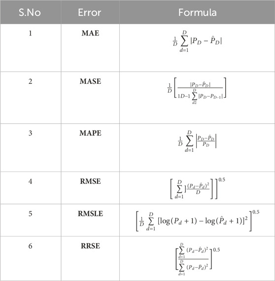
Table 1. Mean evaluation errors.

The table presents the actual $(P_d)$ and forecasted $({\widehat{P}}_d)$ value of ${\text{PM}}_2.5$. Consequently, diminishing values for MAE, MASE, MAPE, RMSE, RRSE, and RMSLE generally signify heightened predictive accuracy of the model.

2.3.2 Equal forecast accuracy test

Second, a statistically equal forecast test, the Diebold–Marino (DM) test (Diebold, 2015), is performed to evaluate the forecasting ensemble time series proposed approach. In the literature, It is used to evaluate time series forecasting models, determining whether the forecast errors from one model are statistically different from another model’s forecast errors (Iftikhar et al., 2023a; Shah et al., 2019; Iftikhar et al., 2023b). To perform the DM test, the forecast errors of each model are calculated using a loss function. Then, a statistical value is computed by comparing the errors of each model. The test statistic is based on the difference between the mean squared errors of the two models. Suppose the test statistic is above a certain threshold and the p-value is below a significance level $(\alpha =0.05)$. In that case, the forecasts from one model are significantly better than the other model. For instance, calculate the forecast errors for both models. Forecast errors $(e_d=P_d-{\widehat{P}}_d)$ are the differences between the observed values $(P_d)$ and the forecasted values $({\widehat{P}}_d)$. Compute the mean difference $(\bar{w})$ of the forecast errors: $\bar{w}=\frac{1}{D}{\sum }_{d=1}^D(e_{1d}-e_{2d})$. Where: $e_{1d}$ and $e_{2d}$ are the forecast errors from Model 1 and Model 2 at time d, respectively, and D is the number of observations. Next, calculate the variance of the differences, such as ${\sigma }_d^2=\frac{1}{D}{\sum }_{d=1}^D{(e_{1d}-e_{2d}-\bar{w})}^2$. Thus, the Diebold-Mariano test statistic DM = $\frac{\bar{w}}{\sqrt{{\sigma }_d^2}}$. Finally, the Null and alternative hypothesized generally state as ${\text{H}}_0$: There is no difference in forecast accuracy between the two models (${\text{H}}_0$: $\bar{w}$ = 0) Vs. ${\text{H}}_A$: The two models differ in forecast accuracy (${\text{H}}_A$: $\bar{w}\ne 0$). Hence, the null hypothesis implies that there is not a statistically significant difference in forecast accuracy between the models. In contrast, the alternative hypothesis suggests a significant difference in forecast accuracy between the two models.

To complete this section, the main steps, including the introduced time series ensemble forecasting approach in bullet form, are listed below, and the flowchart is presented in Figure 1.

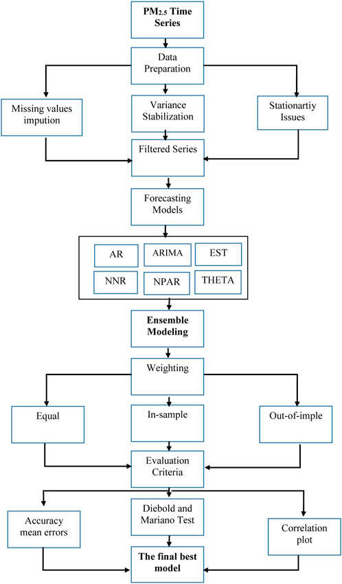
$•$ In the first step, we divide the clean ${\text{PM}}_{2.5}$ time series data into three parts: training (in-sample), validation (evaluation), and testing (out-of-sample) datasets. Let $P_d$; $p=\mathrm{1,2},\cdot ,D$ (1826) is the ${\text{PM}}_{2.5}$ time series. The training (60%, in-sample) dataset is $P_m;m=\mathrm{1,2},\cdot ,M(1096)$, the validation (20%, evaluation) dataset is $P_l;l=\mathrm{1,2},\cdot ,L(365)$, and the testing (20%, out-of-sample) dataset is $P_t;t=\mathrm{1,2},\cdot ,T(365)$ where D (D = M + L + T) is the total data points.

$•$ In the second step, model the train data using single models, i.e., the AR, the ARMA, the ESM, the NPAR, the NNA, and the Theta model.

$•$ In the third step, calculate the one-day-ahead ${\text{PM}}_{2.5}$ forecast using the expanding window technique. The forecast values, ${\widehat{P}}_{D-(M+L+T)}^j$ for $j=\mathrm{1,2},\cdot ,6$, are obtained by the models listed in step 2.

$•$ In the fourth step, the output of a basic ensemble method is mathematically described by Equation 9.

${\widehat{P}}_{D-\left(M+L+T\right)}^j={\displaystyle \sum _{j=1}^6}{\text{W}}_i{\widehat{P}}_{D-\left(M+L+T\right)}^j(9)$

Figure 1

Figure 1. ${\text{PM}}_{2.5}$ modeling and forecasting: A complete proposed time series ensemble approach Layout.

Where ${\text{W}}_i$, are obtained by three weighting strategies: a) equal weight to all single models and denoted by (ESME); b) weight assigned based on training mean accuracy measures (MAPE, MASE, MAE, RMSE, RMSLE, and RRSE) and denoted by (ESMT); c) weight assigned based on validation mean accuracy measures and denoted by (ESMV). The lower accuracy mean errors model assigns more weight to the ensemble model in training and validation data sets. In contrast, the model with the model with the highest accuracy has fewer errors than the ensemble model. However, the model weights are small positive values, and the sum of all weights equals one, indicating the percentage of trust or expected performance from each model. Thus, obtain the day-ahead forecast values using Equation 9 for the ESME, ESMT, and ESMV models.

$•$ In the fifth step, evaluate the model based on average accuracy errors, an equal forecast statistical test, and a graphical assessment (see details in 2.3).

3 Case study results

In order to obtain short-term ${\text{PM}}_{2.5}$ concentration day-ahead forecasts, this study uses the proposed time series ensemble approach to the ${\text{PM}}_{2.5}$ time series data from major cities in Pakistan, including Karachi, Lahore, Peshawar, and Islamabad. The data in this study was collected primarily from air quality data from sensors located at United States embassies across Pakistan (Pakistan, 2021). The datasets for all four cities (Karachi, Lahore, Peshawar, and Islamabad) were recorded daily for 5 years, from 1 June 2019 to 31 May 2023. The considered datasets are described in Table 2, and the location of each city on the Pakistan map has been shown in Figure 2. However, the ${\text{PM}}_{2.5}$ concentration time series generally comprises missing values, high variance, non-normal, and non-stationary. Before modeling and forecasting, these irregularities must be addressed. To tackle these issues, this work first treated the missing values. Multiple imputations imputed the missing data that were considered using the fully conditionally specified. The imputation was done separately for each series (Lahore, Karachi, Peshawar, and Islamabad). The percentage of missing data was between 1.90% and 3.00%, shown in Table 2. However, after getting the imputed ${\text{PM}}_{2.5}$ concentration time series (free of missing data), Figure 3A depicts a graphical representation of all four cities’ imputed daily time series. This figure confirms a long-run linear trend component and an annual seasonality in all four megacities’ time series data.

Table 2

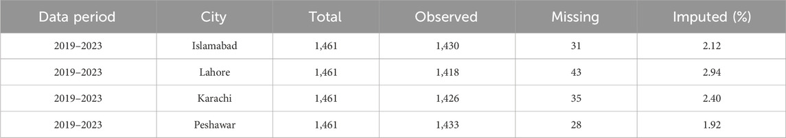
Table 2. Details about the considered original, missing, and imputed datasets are provided in this work.

Figure 2

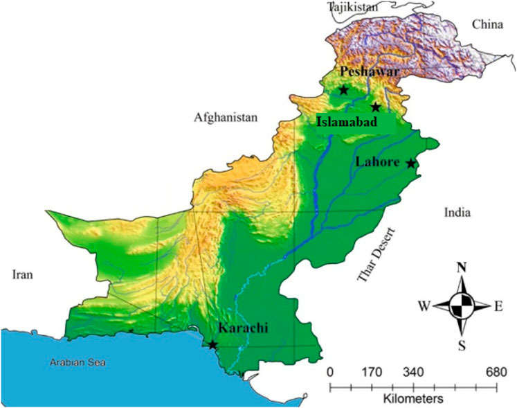
Figure 2. The location of each study city (black star) on the Pakistan map.

Figure 3

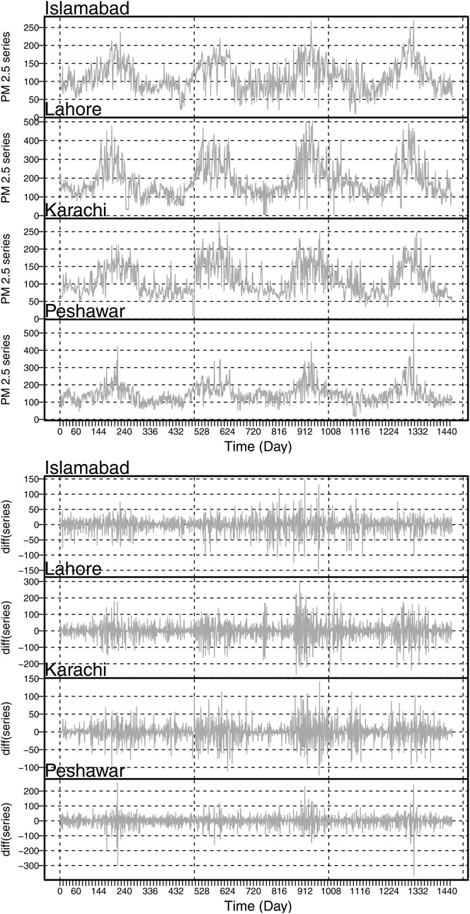
Figure 3. Time Series Plot: Original time series (top) and the first ordered difference time series for all four megacities (bottom).

3.1 Data description

On the other hand, Table 3 represents a comprehensive overview of the statistical properties (with and without log descriptive statistics) for ${\text{PM}}_{2.5}$ concentrations of four cities such as Lahore, Peshawar, Karachi, and Islamabad. As a result, these statistics provide valuable insights into the central tendency, spread, symmetry, and stationarity of the data associated with each city. For instance, as seen in this table, the variance and standard deviation are stabilized by taking the logarithm of each city’s time series. Conversely, the measures of central tendency (mean, median, and mode) indicate that the data is non-normal because the mean, median, and mode are unequal. However, the log series in each case shows the same central tendency, indicating that the series is normal by taking the log to the original series in each case. For example, the mean, median, and model for Islamabad city are approximately the same, taking the log of the ${\text{PM}}_{2.5}$ concentration series. The same experience is experienced in other cities (Lahore, Karachi, and Peshawar). Next, the Augmented Dickey-Fuller (ADF) test is performed to check the non-stationarity issues. The results (the ADF statistic values), listed in Table 3, suggest that both the log-filtered imputed daily ${\text{PM}}_{2.5}$ time series and the log-imputed daily ${\text{PM}}_{2.5}$ time series have a negative statistic value, which indicates that the series is stationary. In addition, the graphical look of all stationary series is plotted in Figure 3B. It can be seen that there is no evidence of nonstationary use in all four megacity time series cases. Once the database addresses all the essential treatments (missing values, variance and standard deviation stabilization, normality, and stationary issues), we proceed further for modeling and forecasting purposes. The dataset was divided into training, validation, and testing datasets. For the daily ${\text{PM}}_{2.5}$ concentration forecast, the training dataset (fitting model) was 3 years (60%) from 1 June 2019 to 31 May 2021, while the validation (validation model, 20%) and testing (testing model, 20%) datasets were one complete year from 1 June 2021 to 31 May 2022 and 1 June 2022 to 31 May 2023, respectively.

Table 3

Table 3. Descriptive statistics.

3.2 ${\text{PM}}_{2.5}$ forecasting outcomes

The given steps must be followed to obtain the forecast for ${\text{PM}}_{2.5}$ concentration one step ahead of a day using the proposed time series ensemble forecasting technique presented in Section 2. First, the time series of ${\text{PM}}_{2.5}$ is preprocessed by missing values and their imputation, variance and standard deviation stabilization, deterministic properties (trend and seasonality), and stationary concerns are addressed. Then, six single time series and three ensemble models anticipate the cleaned ${\text{PM}}_{2.5}$ concentration time series. Therefore, the forecast of a day ahead was obtained using the expanding window technique for 365, and the models were estimated accordingly. Finally, the ${\text{PM}}_{2.5}$ concentration forecasts were achieved through Equation 9. The performance measures, including MAE, MASE, MAPE, RMSE, RRSE, and RMSLE, are then used for the evaluation and comparative performance of the models. Hence, this work uses six single time series models, including the autoregressive model, the exponential smoothing model, the autoregressive moving averages, the nonlinear autoregressive, the neural network autoregressive, and the theta model, and three proposed ensemble models (the ESME, the ESMT, and the ESMV). Thus, the proposed time series ensemble forecasting approach compares nine total models within the two contexts, such as comparing single model performance, the proposed ensemble models, and single verse ensemble models.

Hence, for all nine models for the four monitoring megacities, including Lahore, Islamabad, Karachi, and Peshawar, one-day-ahead out-of-sample forecast outcomes (MAE, MASE, MAPE, RMSE, RRSE, and RMSLE) are listed in Table 4. Table 4 shows that the ESMV produced the best forecasting results compared to all nine forecasting models within the proposed time series ensemble forecasting approach in all four monitoring megacities. For instance, the average accuracy errors for these magacities are the following: Islamabad (MAPE = 0.1739, MAE = 15.2718, MASE = 0.9237, RMSE = 20.3203, RRSE = 0.4830, and RMLSE = 0.2354); Lahore (MAPE = 0.2167, MAE = 34.1786, MASE = 0.9207, RMSE = 48.3090, RRSE = 0.5837, and RMLSE = 0.2701); Karachi (MAPE = 0.1679, MAE = 16.0982, MASE = 0.9122, RMSE = 22.9913, RRSE = 0.5464, and RMLSE = 0.2215); and Peshawar (MAPE = 0.1973, MAE = 24.1188, MASE = 0.8858, RMSE = 35.0552, RRSE = 0.5998, and RMLSE = 0.2594). However, the ESMT model shows the second-best forecasting results among all nine forecasting models in all four monitoring megacities, while the third-best forecasting accuracy average error results are given in the following manner: Islamabad (the Theta model; MAPE = 0.1835, MAE = 16.3457, MASE = 0.9887, RMSE = 21.2335, RRSE = 0.5047, and RMLSE = 0.2370); Lahore (the Theta model; MAPE = 0.2179, MAE = 35.0539, MASE = 0.9442, RMSE = 49.9617, RRSE = 0.6037, and RMLSE = 0.2723); Karachi (the ARMA model; MAPE = 0.1702, MAE = 16.3909, MASE = 0.9287, RMSE = 23.3728, RRSE = 0.5555, RMSLE = 0.2226); and Peshawar (the NPAR model; MAPE = 0.2010, MAE = 25.0597, MASE = 0.9204, RMSE = 36.1912, RRSE = 0.6037, and RMLSE = 0.2723); Karachi (the ARMA model; MAPE = 0.1702, MAE = 16.3909, MASE = 0.9287, RMSE = 23.3728, RRSE = 0.5555, RMSLE = 0.2226); and Peshawar (the NPAR model; MAPE = 0.2010, MAE = 25.0597, MASE = 0.9204, RMSE = 36.1912, RRSE = 0.6192, RMSLE = 0.2610). Therefore, it is seen that within all nine forecasting models, the proposed ensemble models (the ESMV and the ESMT models) generally perform better than single models; however, within the single models, different cities have different single best models, as mentioned previously. Note that the best model is an ESMV or equivalent for all four mountaineering megacities. Also, using the proposed ensemble learning leads to marked error reduction (see Table 4). The proposed ensemble learning approach, thus, proves to be particularly effective in forecasting short-term ${\text{PM}}_{2.5}$ concentration.Once the best models are achieved by average accuracy errors, they are processed to confirm their superiority using a statistical test; for this purpose, this work performs the Diebold and Mariano test (DM). This test is used to check whether two different models performed in the same way or vice versa, and the following hypotheses are tested: the null hypothesis, ${\text{H}}_0$: There is equal accuracy between the models on the rows and columns; the alternative, ${\text{H}}_A$: Compared to the models on the rows, the models on the columns are more accurate. In this way, the hypothesis’s testing is statistically evaluated with the p-value. The models assessed by this test can be interpreted as indicating that the higher the p-value, the better the performance of the specific model. The results (p-values) are demonstrated in Table 5, and the evaluation of these results is based on the row and column in each case. For example, for the Islamabad city in Table 5, it can be noticed that the proposed ensemble model ESMV outperforms the existing models with a value of 0.9120; additionally, for the Lahore station in Table 5, it can be observed that the proposed ensemble model ESMV outputs a significant p-value of 0.900, which shows that the proposed ensemble model is more efficient than others. Furthermore, for the Karachi station in Table 5, it is noticed that the proposed ensemble model shows a significant value of 0.908. In addition to this, for the Peshawar station in Table 5, it can be noticed that the proposed ensemble model results in a p-value of 0.908, which is more significant than other models. Hence, again, it is confirmed by the statistical test that the proposed ensemble model performed better in the prediction of ${\text{PM}}_{2.5}$ than the existing models for all four megacities.

Table 4

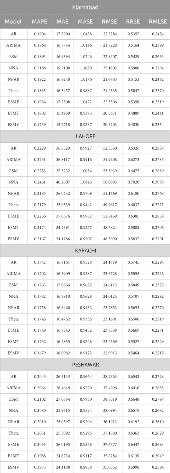
Table 4. The average accuracy errors for all six single models and three proposed ensemble models.

Table 5

Table 5. The DM test outcomes for all six single models and three proposed ensemble models.

On the other hand, after the evaluation of the proposed time series ensemble modeling and forecasting technique by the average mean errors and the DM test, another check can be made to evaluate the accuracy of the selected best ensemble models by the graphical representation of the observed data and the predicted data. To do this, each city’s scatter plot (correlation) is drawn, and the correlation coefficient is calculated. Figures 4A–D shows the graph for each megacity. In Figure 5A for Islamabad city, it is noticed that the correlation coefficient value between the forecasted and actual data set is 0.97, indicating a strong and positive correlation. Moreover, from Figure 4B for Lahore city, the coefficient value between forecasted and actual data is 0.86, which shows a strong positive correlation between forecasted and actual data. Figure 4C for Karachi city and Figure 4D for Peshawar city, the coefficient values are 0.85 and 0.94, which shows a strong positive correlation between forecasted and actual data. In addition, the diagnostic checking (final residuals) plays an essential role in model selection, and this is tracked by the auto-correlation (ACF) plot and the partial auto-correlation plot (PACF), also known as the correlogram plot. As stated earlier, the proposed ensemble model is significant and efficient in forecasting the ${\text{PM}}_{2.5}$ concentration, so the proposed ensemble model ESMV residuals are plotted using correlograms (ACF and PACF plots). In Figure 5, the Figure 5A, C, E, G and Figure 5B, D, F, H plots of four megacities, namely, Islamabad, Lahore, Karachi, and Peshawar, are demonstrated, and the 95% of the confidence interval is calculated, which is shown by the dashed (—) lines for the upcoming lags. This Figure 5 shows that no spike is out of the 95% of the C.I. for all four cities, indicating that the residuals are white noise and the selected model is best for the further statistical perspective, i.e., prediction and forecast.Hence, to sum up this section, based on the evaluation criteria (average mean errors, the statistical test, and the graphical assessment), the proposed time series ensemble forecasting approach is best for efficient and accurate short-term forecasts for ${\text{PM}}_{2.5}$ concentration forecasting. In addition, within the proposed time series ensemble learning approach, the proposed ESMV model produces more precise forecasts when compared with the alternative ensemble models and single time series models.

Figure 4

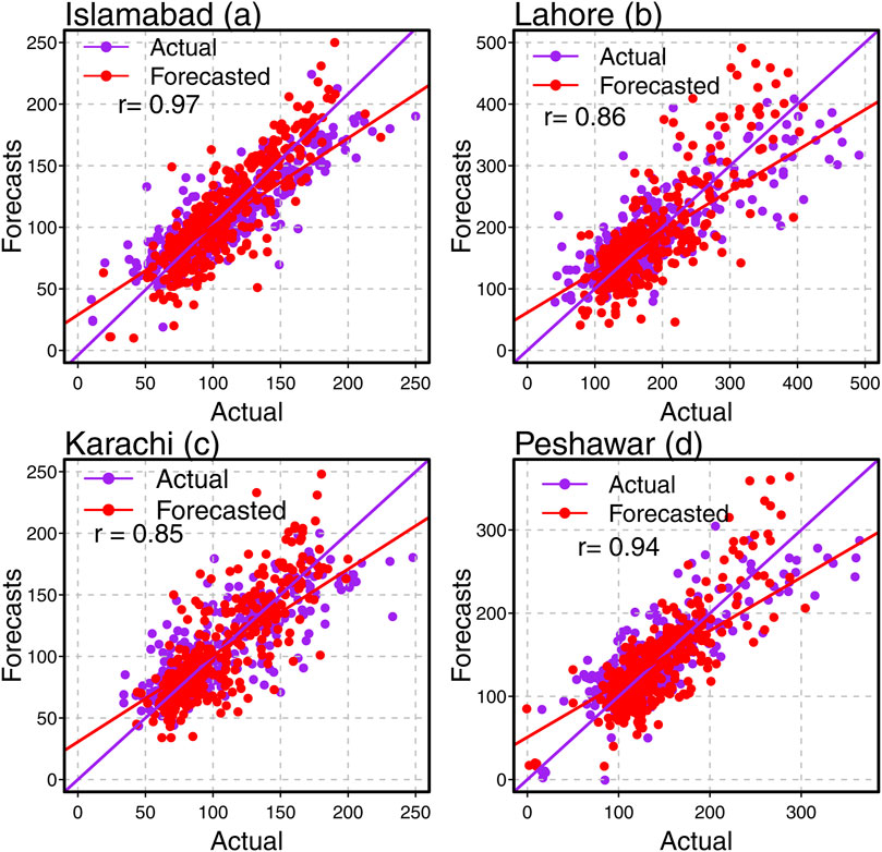
Figure 4. The correlation plots for the best models among all nine considered models in each city: Islamabad (a), Lahore (b), Karachi (c), and Peshawar (d).

Figure 5

Figure 5. The autocorrelation function and partial autocorrelation plots for the best models among all nine considered models in each megacity case: (A, B) Islamabad, (C, D) Lahore, (E, F) Karachi, (G, H) Peshawar.

4 Discussion

This section elaborates an overview of comparing the proposed best model of this work versus the literature that found the best forecasting models. On the other hand, it also explains the future ${\text{PM}}_{2.5}$ forecasting results and directions for the policymaker and health sector precautions.

4.1 Comparatively study resutls

In this subsection, we compared the results of our best ensemble model with those reported in the literature models. Our model showed high comparability with the other methods. Our best (ESMV) model produced the most negligible mean errors and the highest correlation coefficient (MAPE = 0.1679, MAE = 16.0982, MASE = 0.9122, RMSE = 22.9913, RRSE = 0.5464, and RMLSE = 0.2215) compared to the best models reported in the literature. For example, the best autoregressive distributed lag model (the ARDL model) proposed in Qayyum et al. (2021) was applied to the dataset used in our study and showed accuracy measures (MAPE = 0.1835, MAE = 21.3457, MASE = 0.9887, RMSE = 21.2335, RRSE = 0.5047, and RMLSE = 0.2370) that were significantly greater than those of our best (ESMV) model. The best model proposed in another study (see Bhatti et al., 2021) - the seasonal autoregressive moving average factor analysis approach - was also applied to our dataset and obtained average mean errors (MAPE = 0.1823, MAE = 20.1038, MASE = 0.9483, RMSE = 36.1853, RRSE = 0.7214, and RMLSE = 0.2901) that were higher than those of our best (ESMV) model. Similarly, in reference Waseem et al. (2022), the best proposed LSTM encoder-decoder applied to our dataset obtained performance metrics (MAPE = 0.2010, MAE = 25.0597, MASE = 0.9204, RMSE = 36.1912, RRSE = 0.6192, RMSLE = 0.2610) worse than those obtained with our best combination model (ESMV). In conclusion, our study’s best final model (ESMV) showed high efficacy and accuracy compared to the best models reported in the literature.

4.2 Future short-term forecasting using the superior model

On the other hand, once the best models were assessed through average accuracy errors (MAPE, MAE, MASE, RMSLE, RRSE, and RMSE), an equal forecast statistical test (the DM test), graphical evaluation (the ACF, PCAF, and correlogram plots), and comparing with the literature best models this work proceeded to future short-term forecasting with the superior model (the ESMV). In this regard, the current work used the ESMV for the ${\text{PM}}_{2.5}$ concentration and forecast from June 1 to 15 June 2023 (15 days) for the daily ${\text{PM}}_{2.5}$ concentration. The forecasted and actual values of the daily ${\text{PM}}_{2.5}$ concentration are tabulated in Table 5. As seen from this table, the daily ${\text{PM}}_{2.5}$ concentration gradually increased, and the first peak (123.12 $(\mu g/m^3)$) was attained on 9 June 2023; however, after this peak, the forecasts were between 65 $(\mu g/m^3)$ and 110 $(\mu g/m^3)$. In Lahore city’s case, the highest value (236.00 $(\mu g/m^3)$) of ${\text{PM}}_{2.5}$ was observed on 8 June 2023, while the other days also showed higher and worse air quality throughout the 15 days. Conversely, Karachi City has observed moderate ${\text{PM}}_{2.5}$ concentration levels between 50 $(\mu g/m^3)$ and 80 $(\mu g/m^3)$ throughout the next 15 days. In the case of Peshawar City, the ${\text{PM}}_{2.5}$ concentration level was not healthy, and the highest peak was observed on 9 June 2023; however, the other 14 days also showed significant polluted air in the city. As the proposed ensemble model passes all the necessary statistical tests to prove its efficiency over the other existing models that are being compared, the final step is to move towards daily forecasted ${\text{PM}}_{2.5}$ concentration values versus the original ${\text{PM}}_{2.5}$ concentration values of the 15 days (June 1 to 15 June 2023). Table 6 presents the forecasted values for the next 15 days for all four megacities using the proposed model. The percentage forecast error (PFE) is calculated, while the PFE can be defined as PFE = ($\widehat{\text{P}}$ - P/P) * 100. where P is the actual value and $\widehat{P}$ stands for forecasted values. Table 6 gives PFE for each city for the next 15 days. It is found that, on average, the PFE for Islamabad station is 1.04, which is negligible, or stated differently, that this error lies in a 95% confidence interval. Also, for the Karachi station, the PFE on average is 1.12. Moreover, the PFE on average for Lahore station is 0.58, and lastly, for Peshawar station, the PFE on average is 0.51. These, on average, errors prove that the proposed ensemble model forecasts the ${\text{PM}}_{2.5}$ efficiently with the lowest forecast errors.

Table 6

Table 6. Forecasted values exercise for all megacities for the next 15 days using the best model in each case.

As per the Air Quality Index by the Environment Protection Agency, US, the following ranges and their health level concerns: 0–12 $(\mu g/m^3)$, good; 12.1–34.5 $(\mu g/m^3)$, moderate; 34.6–55.4 $(\mu g/m^3)$, unhealthy for sensitive groups; 55.5–150.4 $(\mu g/m^3)$, unhealthy; 150.5–250.4 $(\mu g/m^3)$, very unhealthy; 250.5–350.4 $(\mu g/m^3)$, and hazardous; 350.5–450.4 $(\mu g/m^3)$. In this way, the air quality is classified into different categories for the four megacities of Pakistan based on actual and forecasted values. Islamabad city found that most of the predicted values lie in the fourth class, i.e., $\geqq$ 55.5, which indicates that the air in Islamabad is unhealthy and needs severe precautions for the citizen’s health. Moreover, for Karachi, it is found from the forecasted table that the most values lie in the third class, i.e., $\leqq$ 55.5 $(\mu g/m^3)$, which highlights that the air of the Karachi district is sensitive to some specific groups of people. In addition to this, for Lahore city, the majority of forecasted values lie in the, i.e.,$\leqq$ 55.5 $(\mu g/m^3)$ unhealthy and, i.e., $\leqq$ 150.5 $(\mu g/m^3)$ very unhealthy class of air quality, and lastly, for Peshawar city, the majority of predicted values lie in the suffering class of air quality. Therefore, given that the study demonstrated that ensemble-based time series models could reliably simulate and forecast ${\text{PM}}_{2.5}$ levels, it is suggested that these models be used in real-world scenarios. These models can help decision-making about pollution control and public health by offering insight into future ${\text{PM}}_{2.5}$ levels. Policymakers can benefit from precise ${\text{PM}}_{2.5}$ forecasts when creating efficient pollution management strategies and regulations. To detect trends and patterns and implement timely measures to alleviate pollution and its detrimental impacts on public health, regular monitoring of ${\text{PM}}_{2.5}$ levels in Pakistan’s main cities might be helpful. The study’s findings can be utilized to educate the public about the dangers increased ${\text{PM}}_{2.5}$ levels pose to their health. Public awareness efforts concerning ${\text{PM}}_{2.5}$ pollution can help people decrease their exposure by encouraging them to use air purifiers indoors and stay indoors during high pollution. In summary, this study offers a significant understanding of the modeling and forecasting of ${\text{PM}}_{2.5}$ levels in Pakistan’s main cities, which may guide policy decisions and measures to lower air pollution and safeguard public health.

5 Conclusion

This work proposes a novel time series ensemble approach using the daily ${\text{PM}}_{2.5}$ concentration data from 1 January 2019 to 31 May 2023 from Pakistan’s megacities, including Lahore, Karachi, Peshawar, and Islamabad, to forecast short-term ${\text{PM}}_{2.5}$ concentrations. First, the proposed ensemble approach preprocesses the ${\text{PM}}_{2.5}$ time series by missing value, variance stabilization, normality, deterministic features, and stationary concerns. Second, six single forecasting models: four linear (autoregressive, simple exponential smoothing, autoregressive moving average, and theta) and two nonlinear (nonparametric autoregressive and neural network autoregressive) time series models and three of their ensemble models forecast the cleaned ${\text{PM}}_{2.5}$ concentration time series. The results of six accuracy metrics, the Diebold and Mariano test, and the correlation plot show that the proposed ensemble approach, ESMV, was accurate and efficient for day-ahead ${\text{PM}}_{2.5}$ concentration forecasting. For instance, when the performance of the best ensemble model (ESMV) was compared to all the competitor models (six single models and two other proposed ensemble models) in the four monitoring cities, it was discovered that the model performance had mean errors ranging from 3.60% to 25.79%, 0.81%–13.52%, 1.08%–7.06%, and 1.09%–12.11% in Islamabad, Lahore, Karachi, and Peshawar.

In addition, using the best ensemble model in this work, a forecast was made for the next 15 days (1 June to 15 June 2023); the forecast exercise shows that the elevated levels of ${\text{PM}}_{2.5}$ in major megacities of Pakistan, including Islamabad, Lahore, Karachi, and Peshawar, are suffering from severe air pollution issues. The capital city of Pakistan, Islamabad, is significantly affected by the problem of air pollution, with exceptionally high ${\text{PM}}_{2.5}$ levels, and the leading cause of this pollution belongs to multiple sources, including industrial processes, natural sources, and vehicle emissions. Another significant city in Pakistan, Lahore, has frequently experienced considerable trouble with its air quality, notably in the winter season when variables like temperature inversions and crop burning increase pollution levels. Being a major metropolis and an industrial center, Karachi also suffers from air pollution. The reasons behind this air pollution are the city’s industrial operations, heavy traffic, and trash burning. Peshawar, a capital city in the province of Khyber Pakhtunkhwa, also has air pollution problems, and the same factors, like automobile emissions, manufacturing, and farming practices, cause air pollution. It was found that the factors that pollute the air and make it unhealthy are similar in every city in Pakistan. This polluted air caused smog and irregular moments like accidents and holidays at educational institutions.

However, the study’s main limitation is that it only incorporates ${\text{PM}}_{2.5}$ concentration data and does not include additional exogenous parameters such as temperature, ${\text{PM}}_{10}$, wind speed, ozone concentration, meteorological data, and gas concentrations, which might improve ${\text{PM}}_{2.5}$ forecasting accuracy. On the other hand, the current study employed only data from Pakistani megacities. It may be used in different countries to assess the utility of the proposed time series ensemble modeling and forecasting approach. Furthermore, while this study only employed univariate time series models, machine learning techniques like deep learning and artificial neural networks might be explored within the proposed forecasting framework.

Data availability statement

The original contributions presented in the study are included in the article/supplementary material, further inquiries can be directed to the corresponding author.

Author contributions

HI: Conceptualization, Data curation, Formal Analysis, Investigation, Methodology, Project administration, Resources, Software, Supervision, Validation, Visualization, Writing–original draft, Writing–review and editing. MQ: Data curation, Formal Analysis, Investigation, Writing–review and editing. JZ: Funding acquisition, Project administration, Supervision, Writing–review and editing. JL-G: Investigation, Project administration, Resources, Supervision, Writing–review and editing. OA: Investigation, Resources, Supervision, Writing–review and editing.

Funding

The author(s) declare that no financial support was received for the research, authorship, and/or publication of this article.

Conflict of interest

The authors declare that the research was conducted in the absence of any commercial or financial relationships that could be construed as a potential conflict of interest.

Publisher’s note

All claims expressed in this article are solely those of the authors and do not necessarily represent those of their affiliated organizations, or those of the publisher, the editors and the reviewers. Any product that may be evaluated in this article, or claim that may be made by its manufacturer, is not guaranteed or endorsed by the publisher.

References

Abdullah, S., Ismail, M., Ahmed, A. N., and Abdullah, A. M. (2019). Forecasting particulate matter concentration using linear and non-linear approaches for air quality decision support. Atmosphere 10, 667. doi:10.3390/atmos10110667

CrossRef Full Text | Google Scholar

Alshanbari, H. M., Iftikhar, H., Khan, F., Rind, M., Ahmad, Z., and El-Bagoury, A. A.-A. H. (2023). On the implementation of the artificial neural network approach for forecasting different healthcare events. Diagnostics 13, 1310. doi:10.3390/diagnostics13071310

PubMed Abstract | CrossRef Full Text | Google Scholar

Álvarez-Díaz, M. (2020). Is it possible to accurately forecast the evolution of brent crude oil prices? an answer based on parametric and nonparametric forecasting methods. Empir. Econ. 59, 1285–1305. doi:10.1007/s00181-019-01665-w

CrossRef Full Text | Google Scholar

Ameer, S., Shah, M. A., Khan, A., Song, H., Maple, C., Islam, S. U., et al. (2019). Comparative analysis of machine learning techniques for predicting air quality in smart cities. IEEE Access 7, 128325–128338. doi:10.1109/access.2019.2925082

CrossRef Full Text | Google Scholar

Ashraf, M. U., Akram, F., and Usman, S. (2022). Comparative analysis of machine learning techniques for predicting air pollution. Lahore Garrison Univ. Res. J. Comput. Sci. Inf. Technol. 6, 40–54. doi:10.54692/lgurjcsit.2022.0602270

CrossRef Full Text | Google Scholar

Bai, Y., Zeng, B., Li, C., and Zhang, J. (2019). An ensemble long short-term memory neural network for hourly pm2. 5 concentration forecasting. Chemosphere 222, 286–294. doi:10.1016/j.chemosphere.2019.01.121

PubMed Abstract | CrossRef Full Text | Google Scholar

Bhatti, U. A., Yan, Y., Zhou, M., Ali, S., Hussain, A., Qingsong, H., et al. (2021). Time series analysis and forecasting of air pollution particulate matter (pm 2.5): an sarima and factor analysis approach. Ieee Access 9, 41019–41031. doi:10.1109/access.2021.3060744

CrossRef Full Text | Google Scholar

Borse, S. K. (2020). A review: predicting air quality using different technique. Acta Tech. Corviniensis-Bulletin Eng. 13, 153–157.

Google Scholar

Box, G. E. P., Jenkins, G. M., Reinsel, G. C., and Ljung, G. M. (2015). Time series analysis: forecasting and control. John Wiley and Sons.

Google Scholar

Brown, R. G. (1956). Exponential smoothing for predicting demand. cambridge, mass. NBER Cambridge, MA, United States: arthur d. little. Book exponential smoothing for predicting demand.

Google Scholar

Carbo-Bustinza, N., Iftikhar, H., Belmonte, M., Cabello-Torres, R. J., De La Cruz, A. R. H., and López-Gonzales, J. L. (2023). Short-term forecasting of ozone concentration in metropolitan lima using hybrid combinations of time series models. Appl. Sci. 13, 10514. doi:10.3390/app131810514

CrossRef Full Text | Google Scholar

Chen, G., Kuang, R., Li, W., Cui, K., Fu, D., Yang, Z., et al. (2024). Numerical study on efficiency and robustness of wave energy converter-power take-off system for compressed air energy storage. Renew. Energy 121080.

CrossRef Full Text | Google Scholar

Chen, J., Chen, H., Wu, Z., Hu, D., and Pan, J. Z. (2017). Forecasting smog-related health hazard based on social media and physical sensor. Inf. Syst. 64, 281–291. doi:10.1016/j.is.2016.03.011

PubMed Abstract | CrossRef Full Text | Google Scholar

Diebold, F. X. (2015). Comparing predictive accuracy, twenty years later: a personal perspective on the use and abuse of diebold–mariano tests. J. Bus. and Econ. Statistics 33, 1. doi:10.1080/07350015.2014.983236

CrossRef Full Text | Google Scholar

Donahue, N. M. (2018). “Air pollution and air quality,” in Green chemistry (Elsevier), 151–176.

CrossRef Full Text | Google Scholar

Du, W., and Wang, G. (2013). Intra-event spatial correlations for cumulative absolute velocity, arias intensity, and spectral accelerations based on regional site conditions. Bull. Seismol. Soc. Am. 103, 1117–1129. doi:10.1785/0120120185

CrossRef Full Text | Google Scholar

Dutta, A., and Jinsart, W. (2021). Air pollution in indian cities and comparison of mlr, ann and cart models for predicting pm10 concentrations in guwahati, India. Asian J. Atmos. Environ. 15, 2020131. doi:10.5572/ajae.2020.131

CrossRef Full Text | Google Scholar

Ejohwomu, O. A., Shamsideen Oshodi, O., Oladokun, M., Bukoye, O. T., Emekwuru, N., Sotunbo, A., et al. (2022). Modelling and forecasting temporal pm2. 5 concentration using ensemble machine learning methods. Buildings 12, 46. doi:10.3390/buildings12010046

CrossRef Full Text | Google Scholar

Freeman, B. S., Taylor, G., Gharabaghi, B., and Thé, J. (2018). Forecasting air quality time series using deep learning. J. Air and Waste Manag. Assoc. 68, 866–886. doi:10.1080/10962247.2018.1459956

PubMed Abstract | CrossRef Full Text | Google Scholar

Garg, S., and Jindal, H. (2021). “Evaluation of time series forecasting models for estimation of pm2. 5 levels in air,” in 2021 6th international conference for convergence in technology I2CT (IEEE), 1–8.

CrossRef Full Text | Google Scholar

Geetha, S., and Prasika, L. (2019). Smog prediction model using time series with long-short term memory. Int. J. Mech. Eng. Technol. 10, 1026–1032.

Google Scholar

Gonzales, S. M., Iftikhar, H., and López-Gonzales, J. L. (2024). Analysis and forecasting of electricity prices using an improved time series ensemble approach: an application to the peruvian electricity market. AIMS Math. 9, 21952–21971. doi:10.3934/math.20241067

CrossRef Full Text | Google Scholar

Holt, C. C. (2004). Forecasting seasonals and trends by exponentially weighted moving averages. Int. J. Forecast. 20, 5–10. doi:10.1016/j.ijforecast.2003.09.015

CrossRef Full Text | Google Scholar

Iftikhar, H., Bibi, N., Canas Rodrigues, P., and López-Gonzales, J. L. (2023a). Multiple novel decomposition techniques for time series forecasting: application to monthly forecasting of electricity consumption in Pakistan. Energies 16, 2579. doi:10.3390/en16062579

CrossRef Full Text | Google Scholar

Iftikhar, H., Gonzales, S. M., Zywiołek, J., and López-Gonzales, J. L. (2024a). Electricity demand forecasting using a novel time series ensemble technique. IEEE Access 12, 88963–88975. doi:10.1109/access.2024.3419551

CrossRef Full Text | Google Scholar

Iftikhar, H., Khan, M., Turpo-Chaparro, J. E., Rodrigues, P. C., and López-Gonzales, J. L. (2024b). Forecasting stock prices using a novel filtering-combination technique: application to the Pakistan stock exchange. AIMS Math. 9, 3264–3288. doi:10.3934/math.2024159

CrossRef Full Text | Google Scholar

Iftikhar, H., Khan, M., Żywiołek, J., Khan, M., and López-Gonzales, J. L. (2024c). Modeling and forecasting carbon dioxide emission in Pakistan using a hybrid combination of regression and time series models. Heliyon 10, e33148. doi:10.1016/j.heliyon.2024.e33148

CrossRef Full Text | Google Scholar

Iftikhar, H., Turpo-Chaparro, J. E., Canas Rodrigues, P., and López-Gonzales, J. L. (2023b). Day-ahead electricity demand forecasting using a novel decomposition combination method. Energies 16, 6675. doi:10.3390/en16186675

CrossRef Full Text | Google Scholar

Iftikhar, H., Turpo-Chaparro, J. E., Canas Rodrigues, P., and López-Gonzales, J. L. (2023c). Forecasting day-ahead electricity prices for the Italian electricity market using a new decomposition—combination technique. Energies 16, 6669. doi:10.3390/en16186669

CrossRef Full Text | Google Scholar

Iftikhar, H., Zafar, A., Turpo-Chaparro, J. E., Canas Rodrigues, P., and López-Gonzales, J. L. (2023d). Forecasting day-ahead brent crude oil prices using hybrid combinations of time series models. Mathematics 11, 3548. doi:10.3390/math11163548

CrossRef Full Text | Google Scholar

Jenkins, G. M., and Box, G. E. P. (1976). Time series analysis: forecasting and control. Hoboken, New Jersey, United States: Prentice Hall.

Google Scholar

Kleine Deters, J., Zalakeviciute, R., Gonzalez, M., and Rybarczyk, Y. (2017). Modeling pm 2.5 urban pollution using machine learning and selected meteorological parameters. J. Electr. Comput. Eng. 2017, 1–14. doi:10.1155/2017/5106045

CrossRef Full Text | Google Scholar

Lin, H.-X., Jin, J., and van den Herik, H. J. (2019). Air quality forecast through integrated data assimilation and machine learning. ICAART 2, 787–793.

CrossRef Full Text | Google Scholar

Liu, D.-R., Lee, S.-J., Huang, Y., and Chiu, C.-J. (2020). Air pollution forecasting based on attention-based lsm neural network and ensemble learning. Expert Syst. 37, e12511. doi:10.1111/exsy.12511

CrossRef Full Text | Google Scholar

Luo, J., Zhuo, W., Liu, S., and Xu, B. (2024). The optimization of carbon emission prediction in low carbon energy economy under big data. IEEE Access 12, 14690–14702. doi:10.1109/access.2024.3351468

CrossRef Full Text | Google Scholar

Manisalidis, I., Stavropoulou, E., Stavropoulos, A., and Bezirtzoglou, E. (2020). Environmental and health impacts of air pollution: a review. Front. public health 8, 14. doi:10.3389/fpubh.2020.00014

PubMed Abstract | CrossRef Full Text | Google Scholar

Pakistan, U. C. (2021). Air quality data. The U.S. Environmental Protection Agency, Washington, D.C.: US Consulate Pakistan.

Google Scholar

Qayyum, F., Mehmood, U., Tariq, S., Haq, Z. u., and Nawaz, H. (2021). Particulate matter (pm2. 5) and diseases: an autoregressive distributed lag (ardl) technique. Environ. Sci. Pollut. Res. 28, 67511–67518. doi:10.1007/s11356-021-15178-6

CrossRef Full Text | Google Scholar

Qiu, L., Xia, W., Wei, S., Hu, H., Yang, L., Chen, Y., et al. (2024). Collaborative management of environmental pollution and carbon emissions drives local green growth: an analysis based on spatial effects. Environ. Res. 259, 119546. doi:10.1016/j.envres.2024.119546

PubMed Abstract | CrossRef Full Text | Google Scholar

Quispe, F., Salcedo, E., Iftikhar, H., Zafar, A., Khan, M., Turpo-Chaparro, J. E., et al. (2024). Multi-step ahead ozone level forecasting using a component-based technique: a case study in lima, Peru. AIMS Environ. Sci. 11, 401–425. doi:10.3934/environsci.2024020

CrossRef Full Text | Google Scholar

Rakholia, R., Le, Q., Ho, B. Q., Vu, K., and Carbajo, R. S. (2023). Multi-output machine learning model for regional air pollution forecasting in ho chi min city, vietnam. Environ. Int. 173, 107848. doi:10.1016/j.envint.2023.107848

PubMed Abstract | CrossRef Full Text | Google Scholar

Shah, I., Iftikhar, H., and Ali, S. (2020). Modeling and forecasting medium-term electricity consumption using component estimation technique. Forecasting 2, 163–179. doi:10.3390/forecast2020009

CrossRef Full Text | Google Scholar

Shah, I., Iftikhar, H., and Ali, S. (2022). Modeling and forecasting electricity demand and prices: a comparison of alternative approaches. J. Math. 2022, 3581037. doi:10.1155/2022/3581037

CrossRef Full Text | Google Scholar

Shah, I., Iftikhar, H., Ali, S., and Wang, D. (2019). Short-term electricity demand forecasting using components estimation technique. Energies 12, 2532. doi:10.3390/en12132532

CrossRef Full Text | Google Scholar

Shang, K., Xu, L., Liu, X., Yin, Z., Liu, Z., Li, X., et al. (2023). Study of urban heat island effect in Hangzhou metropolitan area based on sw-tes algorithm and image dichotomous model. Sage Open 13, 21582440231208851. doi:10.1177/21582440231208851

CrossRef Full Text | Google Scholar

Shang, M., and Luo, J. (2021). The tapio decoupling principle and key strategies for changing factors of Chinese urban carbon footprint based on cloud computing. Int. J. Environ. Res. Public Health 18, 2101. doi:10.3390/ijerph18042101

PubMed Abstract | CrossRef Full Text | Google Scholar

Taskaya-Temizel, T., and Casey, M. C. (2005). A comparative study of autoregressive neural network hybrids. Neural Netw. 18, 781–789. doi:10.1016/j.neunet.2005.06.003

PubMed Abstract | CrossRef Full Text | Google Scholar

Ullah, S., Ullah, N., Rajper, S. A., Ahmad, I., and Li, Z. (2021). Air pollution and associated self-reported effects on the exposed students at malakand division, Pakistan. Environ. Monit. Assess. 193, 708–717. doi:10.1007/s10661-021-09484-2

PubMed Abstract | CrossRef Full Text | Google Scholar

Van Buuren, S., and Oudshoorn, C. G. M. (2011). Mice: multivariate imputation by chained equations inR. J. Stat. Softw. 45, 1–67. doi:10.18637/jss.v045.i03

CrossRef Full Text | Google Scholar

Wang, B., Kong, W., Guan, H., and Xiong, N. N. (2019). Air quality forecasting based on gated recurrent long short term memory model in internet of things. IEEE Access 7, 69524–69534. doi:10.1109/access.2019.2917277

CrossRef Full Text | Google Scholar

Waseem, K. H., Mushtaq, H., Abid, F., Abu-Mahfouz, A. M., Shaikh, A., Turan, M., et al. (2022). Forecasting of air quality using an optimized recurrent neural network. Processes 10, 2117. doi:10.3390/pr10102117

CrossRef Full Text | Google Scholar

Xie, X., Xie, B., Cheng, J., Chu, Q., and Dooling, T. (2021). A simple Monte Carlo method for estimating the chance of a cyclone impact. Nat. Hazards 107, 2573–2582. doi:10.1007/s11069-021-04505-2

CrossRef Full Text | Google Scholar

Xu, J., Zhou, G., Su, S., Cao, Q., and Tian, Z. (2022). The development of a rigorous model for bathymetric mapping from multispectral satellite-images. Remote Sens. 14, 2495. doi:10.3390/rs14102495

CrossRef Full Text | Google Scholar

Xu, Y., Ho, H. C., Wong, M. S., Deng, C., Shi, Y., Chan, T.-C., et al. (2018). Evaluation of machine learning techniques with multiple remote sensing datasets in estimating monthly concentrations of ground-level pm2. 5. Environ. Pollut. 242, 1417–1426. doi:10.1016/j.envpol.2018.08.029

PubMed Abstract | CrossRef Full Text | Google Scholar

Yin, Z., Liu, Z., Liu, X., Zheng, W., and Yin, L. (2023). Urban heat islands and their effects on thermal comfort in the us: New york and New Jersey. Ecol. Indic. 154, 110765. doi:10.1016/j.ecolind.2023.110765

CrossRef Full Text | Google Scholar

Zaman, N. A. F. K., Kanniah, K. D., Kaskaoutis, D. G., and Latif, M. T. (2021). Evaluation of machine learning models for estimating pm2. 5 concentrations across Malaysia. Appl. Sci. 11, 7326. doi:10.3390/app11167326

CrossRef Full Text | Google Scholar

Zaman, N. A. F. K., Kanniah, K. D., Kaskaoutis, D. G., and Latif, M. T. (2024). Improving the quantification of fine particulates (pm2. 5) concentrations in Malaysia using simplified and computationally efficient models. J. Clean. Prod. 448, 141559. doi:10.1016/j.jclepro.2024.141559

CrossRef Full Text | Google Scholar

Zhan, Y., Luo, Y., Deng, X., Chen, H., Grieneisen, M. L., Shen, X., et al. (2017). Spatiotemporal prediction of continuous daily pm2. 5 concentrations across China using a spatially explicit machine learning algorithm. Atmos. Environ. 155, 129–139. doi:10.1016/j.atmosenv.2017.02.023

CrossRef Full Text | Google Scholar

Zhou, G., Lin, G., Liu, Z., Zhou, X., Li, W., Li, X., et al. (2023). An optical system for suppression of laser echo energy from the water surface on single-band bathymetric lidar. Opt. Lasers Eng. 163, 107468. doi:10.1016/j.optlaseng.2022.107468

CrossRef Full Text | Google Scholar

Zhu, C. (2023). An adaptive agent decision model based on deep reinforcement learning and autonomous learning. J. Logist. Inf. Serv. Sci. 10 (3).

Google Scholar