
95% of researchers rate our articles as excellent or good
Learn more about the work of our research integrity team to safeguard the quality of each article we publish.
Find out more
ORIGINAL RESEARCH article
Front. Environ. Sci. , 08 August 2024
Sec. Toxicology, Pollution and the Environment
Volume 12 - 2024 | https://doi.org/10.3389/fenvs.2024.1440296
 Yajie Liang1,2*
 Jieyu Zhao1,2Yiting Zhang1,2Jisheng Li3Jieran Ding1,2Changyong Jing1,2Jiukun Ji1Dongtan Wu1
Introduction: Soil pollution, which includes a variety of contaminants such as heavy metals and organic compounds, poses significant environmental and health risks, making effective prediction and assessment techniques essential. Current predictive models often struggle with the complexity and diversity of soil contaminant behaviors, leading to limitations in their accuracy and applicability.
Methods: Recognizing the importance of capturing the temporal dynamics influenced by seasonal variations and agricultural practices, our study introduces an SSA-optimized Attention-ConvGRU model. This model integrates convolutional neural networks, gated recurrent units, and attention mechanisms, enhanced through optimization with the Sparrow Search Algorithm to improve predictive performance.
Results: Experimental results confirm that our model significantly outperforms traditional methods, demonstrating over 30% improvement in prediction accuracy across multiple datasets.
Discussion: This research underscores the potential of advanced machine learning techniques to revolutionize the assessment of soil pollution, providing substantial benefits for environmental management and public health protection.
Soil is an essential component of the Earth’s system, providing support for human production and life through its production, regulation, cycling, and habitat functions. It plays a critical role in environmental regulation by purifying pollutants to protect the environment Gautam et al. (2023); Raimi et al. (2022). However, rapid industrialization and urbanization have led to severe soil pollution, threatening ecosystems and human health. Soil pollutants include various chemicals such as heavy metals, organic pollutants, and pesticide residues, originating from industrial production, agricultural activities, urbanization processes, and other human activities Wu et al. (2022); Ren and Wang (2024). Soil pollution has a wide range and a broad impact, and its consequences may include declining soil quality, inhibited plant growth, groundwater pollution, and human health issues. Therefore, effectively predicting and assessing the distribution and diffusion of soil pollutants has become an important task for environmental protection and human health. Despite extensive research in the field of soil pollution, the diversity in the nature and behavior of soil pollutants, along with the complexity of the soil environment, poses significant challenges in predicting and assessing soil pollution Wang et al. (2022, 2024). Different pollutants interact and diffuse in soil in various ways, and factors such as soil heterogeneity, seasonal variations, and topographic features further complicate the development of effective prediction models Liu et al. (2023). With the development of deep learning technology, researchers have begun to utilize deep learning methods to study soil pollution issues. Compared to traditional statistical methods and machine learning methods, deep learning has stronger modeling capabilities and better generalization abilities, allowing it to learn complex nonlinear relationships from large amounts of data Gao et al. (2022); Janga et al. (2023). Therefore, deep learning has shown tremendous potential in the prediction and assessment of soil pollutants. Researchers have proposed numerous deep learning-based models to predict the distribution, diffusion, and risk assessment of soil pollutants. These models not only enhance the accuracy of predictions but also speed up the prediction process, providing crucial support for the management and remediation of soil pollution issues Tao et al. (2022); Jiang et al. (2022).
Researchers have proposed various deep learning-based models for predicting analysis and risk assessment of soil pollutants. One of these is based on Convolutional Neural Networks (CNN), which extracts features from spatiotemporal data of soil pollutants through convolutional operations for prediction Mei et al. (2022). While CNNs have certain advantages in feature extraction, their structural characteristics may overlook temporal information in the data, thereby limiting the accuracy of predictions to some extent. Another study employs Long Short-Term Memory networks (LSTM) as the foundational model Zheng et al. (2022). LSTMs play a crucial role in enhancing predictions of the spatiotemporal distribution of soil pollutants by effectively capturing long-term dependencies in time series data. However, despite partially addressing temporal dependencies, LSTM’s modeling capability for long-term dependencies may still be insufficient, resulting in certain limitations in predictions. Another approach involves using Variational Autoencoders (VAE) for soil pollutant prediction Shin et al. (2023). VAEs learn the latent representation of data and generate new samples with similar distributions. While this model has advantages in capturing data distributions, its performance in handling soil pollutants may be affected by data sparsity and noise, leading to decreased prediction accuracy. The last study combines attention mechanisms and Gated Recurrent Units (GRU) Mirzavand Borujeni et al. (2023). This model dynamically weights input data using attention mechanisms and captures long-term dependencies in sequence data using GRU. While this model improves prediction performance to some extent, its modeling of complex relationships between different types of pollutants still requires improvement.
In summary, these studies have made progress in predicting soil pollutants, but there are still some shortcomings. Models may overlook crucial temporal information in spatiotemporal data, and there is room for improvement in modeling long-term dependencies and the complex relationships between different types of pollutants Cui et al. (2023). Therefore, further research and improvement of deep learning models are needed to accurately predict the spatiotemporal distribution of soil pollutants and provide more effective support for environmental protection and soil remediation.
Although these studies have made some progress in predicting soil pollutants, there are still some shortcomings. Current models may overlook critical temporal information when handling spatiotemporal data, have limited capability in modeling long-term dependencies, and need improvement in capturing the complex relationships between different types of pollutants. Therefore, further research and refinement of deep learning models are needed to more accurately predict the spatiotemporal distribution of soil pollutants and provide more effective support for environmental protection and soil remediation.
Based on the identified shortcomings, we propose an attention-ConvGRU model optimized with the Sparrow Search Algorithm (SSA). This model utilizes SSA to optimize parameter settings, aiming to enhance model performance and convergence speed. Additionally, the model integrates attention mechanisms, convolutional Gated Recurrent Unit (ConvGRU) to address challenges in soil pollutant prediction. Within this model, attention mechanisms dynamically weight input data, allowing the model to focus on information relevant to the prediction target, thus improving prediction accuracy. CNNs are employed to extract spatiotemporal features from input data, aiding in capturing spatial distributions and temporal variations of soil pollutants. GRUs handle time-series data, proficiently capturing long-term dependencies among data points and enhancing the model’s ability to model temporal dynamics.
The introduction of our model holds significant importance. By leveraging the SSA algorithm to optimize model parameters, we are able to accelerate the model’s convergence process, thereby enhancing training efficiency. Moreover, the integration of attention mechanisms, convolutional neural networks, and gated recurrent units enables the model to fully exploit the spatiotemporal information of soil pollutant data, leading to improved prediction accuracy and stability. Consequently, our model shows promising prospects for applications in soil pollutant prediction and risk assessment, offering more effective support for environmental protection and soil remediation efforts.
The SSA-optimized attention-ConvGRU model contributes significantly to three aspects in the field of soil pollutant prediction and risk assessment.
In terms of traditional methods for predicting soil pollutants, previous scholars have employed various approaches for research and prediction. These methods often rely on empirical models Zeng et al. (2022), statistical techniques Baragaño et al. (2022), and Geographic Information System (GIS) technology Khan et al. (2022)to forecast the distribution and diffusion of soil pollutants. Empirical models are a common approach, which are based on historical data and expert knowledge to predict future soil pollution scenarios by summarizing and generalizing past experiences. However, empirical models often lack adaptability and precision when dealing with complex, non-linear interactions among multiple soil pollutants and environmental factors. Statistical methods are also widely used, including regression analysis Bijitha and Nath (2022); Zhao et al. (2023), variance analysis, cluster analysis, etc., to establish mathematical models describing the distribution patterns and influencing factors of soil pollutants through statistical analysis of existing data. Despite their usefulness, statistical methods can be limited by the quality and quantity of available data and may not fully capture the dynamic and heterogeneous nature of soil pollution. Furthermore, Geographic Information System (GIS) technology plays a crucial role in soil pollutant prediction, integrating spatial data, topographic information, soil properties, and other multi-source data to build spatial databases and conduct spatial analysis, thereby revealing distribution patterns and spatial correlations of soil pollutants Xu and Zhang (2023); Liu et al. (2022). GIS-based models, while powerful in spatial analysis, often require extensive and high-quality spatial data, which can be challenging to obtain and maintain. Additionally, geostatistical methods combine principles of geology and statistics to model and predict the spatial distribution of soil pollutants Yao and Liu (2024). These methods utilize statistical analysis of geological data to explore the spatial variations of soil pollutants and make spatial predictions Chelabi et al. (2022). However, geostatistical methods may struggle with the spatial autocorrelation and non-stationarity often present in soil pollution data.
In summary, traditional methods for predicting soil pollutants encompass various techniques, including empirical models, statistical methods, GIS technology, and geostatistical methods. While these methods play an important role in revealing distribution patterns of soil pollutants and forecasting future trends, they each have inherent limitations that can affect their accuracy and applicability. These limitations include issues with adaptability, data quality requirements, and the ability to capture complex interactions and dynamics in soil pollution. Therefore, there is a need for more advanced and flexible modeling approaches that can address these challenges and provide more reliable predictions for soil environmental management and protection.
In past research, soil pollutant prediction based on Convolutional Neural Networks (CNNs) has garnered widespread attention Li et al. (2022). CNNs, as powerful deep learning models, have achieved significant success in fields such as image processing and spatial data analysis Pisal and Vidyarthi (2023). When applied to soil pollutant prediction, CNNs excel at effectively extracting features from spatiotemporal soil data, enabling precise prediction of soil pollutants.
CNN models firstly leverage multiple layers of convolution and pooling operations to automatically learn features from spatiotemporal soil data Zhang et al. (2023). These features, including soil properties, topographical features, and environmental factors, help the model better understand the distribution patterns of soil pollutants Siddthan and Shanthi (2022); Liu et al. (2023). By extracting these features, CNNs can uncover hidden patterns and trends within large-scale soil data, thereby improving prediction accuracy and reliability. However, CNNs primarily focus on local spatial features and may struggle to capture long-range dependencies in the data. This limitation can reduce the accuracy of predictions in complex soil environments where such dependencies are significant. Secondly, CNN models possess strong spatial awareness and local connectivity, allowing them to fully consider the spatial distribution characteristics of soil data Nadiri et al. (2022). This enables CNNs to better capture spatial variations of soil pollutants, leading to more accurate predictions of soil pollution under different regional and terrain conditions. Nonetheless, the performance of CNNs can be highly dependent on the quality and quantity of training data, which might not always be available, potentially leading to overfitting or underfitting issues. Moreover, CNNs can be combined with other deep learning models such as Recurrent Neural Networks (RNNs) or Gated Recurrent Units (GRUs) to further enhance model performance Gonzalez et al. (2022); Duan et al. (2022). By integrating multiple deep learning models, their respective strengths can be fully utilized, enabling more precise prediction and comprehensive analysis of soil pollutants.
In conclusion, while soil pollutant prediction based on Convolutional Neural Networks holds significant potential and practical value, it is important to address the inherent limitations of CNNs. These include challenges in capturing long-range dependencies, dependency on high-quality data, and computational complexity. By leveraging information from spatiotemporal soil data and combining powerful feature extraction and spatial awareness capabilities, CNN models can provide more effective methods and tools for predicting and evaluating soil pollutants, thus offering crucial support for environmental protection and soil remediation efforts. Future research should focus on overcoming these limitations to fully realize the potential of CNN-based models in this domain.
This study proposes an attention-ConvGRU model optimized with the Sparrow Search Algorithm (SSA) for predicting and assessing the risk of soil pollutants. This model integrates attention mechanisms, Convolutional Gated Recurrent Units (ConvGRU), and the Sparrow Search Algorithm (SSA). The attention mechanism enables the model to focus more on features relevant to soil pollution prediction, thereby enhancing accuracy and generalization. ConvGRU captures the spatiotemporal characteristics of soil pollution data, aiding the model in effectively analyzing the spatial distribution and temporal changes of soil pollution. The Sparrow Search Algorithm is employed for optimizing model parameters, improving training efficiency and prediction accuracy. In the process of network construction, soil data is first processed through the attention mechanism to extract important features. These characteristics are subsequently input into the ConvGRU unit to capture temporal connections and spatial interdependencies within the data. Subsequently, SSA is employed to optimize the weights and biases of the entire network, ensuring that the model achieves optimal prediction performance after multiple iterations of training. Through this approach, the model not only enhances its ability to identify existing pollution levels but also improves its capability to predict future pollution trends. The overall flowchart is illustrated in Figure 1.
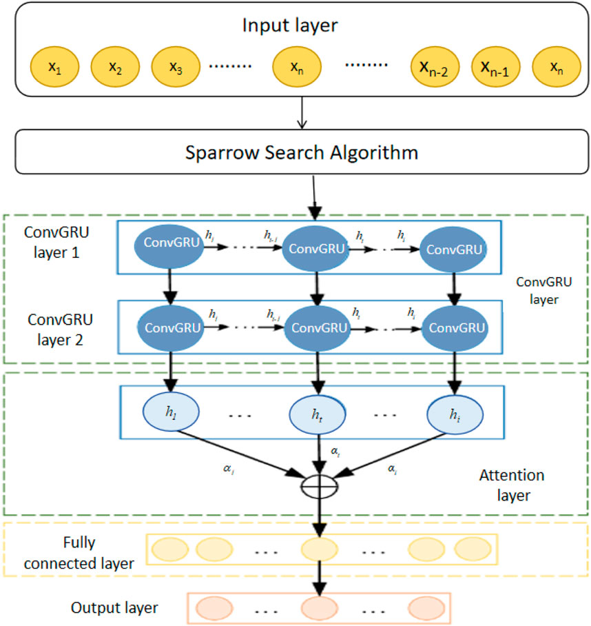
Figure 1. Overall flow chart of the SSA based attention-ConvGRU.
The application of this model is significant for soil pollutant detection as it accurately predicts the concentration changes of various pollutants in soil. This aids environmental scientists and policymakers in more effectively assessing soil pollution risks and formulating corresponding prevention and control measures. By deeply analyzing the spatial distribution and temporal trends of soil pollution, this model contributes to more accurately guiding the implementation of soil remediation and pollution prevention strategies.
The Sparrow Search Algorithm (SSA) is a heuristic optimization algorithm inspired by the foraging behavior of sparrows. In this algorithm, sparrows represent candidate solutions, and the sparrows within a population collectively search the solution space of a problem. SSA achieves efficient global search and parameter optimization by simulating both individual behaviors and collective cooperation among sparrows during foraging Gharehchopogh et al. (2023). The foraging process in SSA consists of four stages: searching, pursuing, tracking, and scouting. During the searching stage, sparrows select food sources based on their own experience and information from neighboring sparrows, adjusting their search direction according to the richness of the food Awadallah et al. (2023). In the pursuing stage, sparrows follow companions that discover more food and attempt to find additional food in the same direction. During the tracking stage, sparrows adjust their flight speed and direction to better follow other sparrows. Finally, in the scouting stage, sparrows explore new food sources through random flights to ensure diversity and exploration within the entire population. By simulating these behaviors, SSA efficiently conducts global search and parameter optimization. In optimization problems, SSA effectively explores the solution space and finds better solutions in shorter timeframes. The algorithmic flowchart for SSA is depicted in Figure 2. The core mathematical formulas related to SSA are presented in Table1 below.
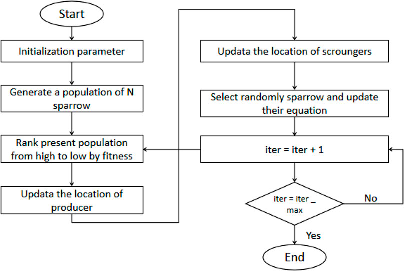
Figure 2. Flow chart of the SSA.

Table 1. Core mathematical formulas related to SSA.
These formulas outline the key components and operations of the SSA algorithm, including the objective function, position update, fitness calculation, leader sparrow update, and stopping criterion.
In our model, the SSA algorithm is utilized to optimize the parameters of the entire model, including the weights of CNN, GRU, and attention mechanisms, as well as the selection of hyperparameters. Through optimization with the SSA algorithm, we can quickly find the optimal parameter configuration for the model, thereby improving both training speed and performance. Moreover, the SSA algorithm aids in better exploration of the parameter space, leading to more stable and reliable models. This enhances the accuracy and robustness of our model in detecting soil pollutants. Thus, the SSA algorithm plays a crucial role in our model, providing an effective means for optimization and performance enhancement.
Attention is a pivotal mechanism designed to enhance the capacity of neural networks in processing sequential data. This mechanism allows the network to selectively focus on the most relevant segments of the input sequence, which in turn significantly improves the model’s performance and accuracy. The fundamental principle of the attention mechanism involves calculating a set of weights for each position in the input sequence Guo et al. (2022). These weights reflect the importance of each part of the sequence in relation to the task at hand. By dynamically adjusting its focus based on these learned weights, the model can prioritize more critical information while disregarding less relevant data. This selective focus enables the model to better capture and understand complex patterns within the sequence, thereby enhancing its overall effectiveness in tasks such as language translation, image captioning, and time-series prediction. The attention mechanism operates by computing a weighted sum of all positions in the input sequence, where the weights are determined by the similarity between a query vector (representing the current position) and key vectors (representing all positions in the sequence). This approach allows the model to flexibly integrate contextual information from the entire sequence, leading to more informed and accurate predictions.
Query-Attention Score: The query-attention score measures the similarity between a query vector and a key vector.
where:
Softmax Attention Weights: The softmax attention weights determine the importance of each key based on their attention scores.
where:
Weighted Sum of Values: The weighted sum of values combines the values with their corresponding softmax attention weights.
where:
Scaled dot-product attention: Scaled dot-product attention is a specific type of attention mechanism that computes the attention scores using the dot product of query and key vectors, scaled by a factor to prevent extremely large values that can hinder the softmax function’s performance. It is formulated as follows:
where
where
Multi-Head Attention: Multi-head attention computes multiple attention heads in parallel, allowing the model to focus on different parts of the input.
where:
In our model, Attention is applied to the task of predicting soil pollutants. By incorporating the Attention mechanism, our model can more flexibly identify and utilize key information within the input data, thereby boosting prediction accuracy and robustness. Particularly, Attention enables the model to prioritize regions of the input sequence that have a significant impact on the prediction of soil pollutants while effectively suppressing irrelevant information. As a result, the model can more accurately capture the distribution patterns and trends of soil pollutants, contributing to a more precise understanding of their spatial and temporal variations.
The Convolutional Gated Recurrent Unit (ConvGRU) is a model that integrates Convolutional Neural Networks (CNNs) and Gated Recurrent Units (GRUs). Its basic principle involves using CNN’s convolutional operations to extract spatial features from sequential data and combining GRU’s gated mechanism to capture temporal features, enabling effective modeling and prediction of sequential data Zhou et al. (2024). In the ConvGRU model, convolutional layers are utilized to extract spatial features from the input data. Convolutional operations enable the model to capture local features and spatial relationships within the data efficiently. These operations are particularly effective for processing data with spatial structures, such as images or spatially organized sequences. On the other hand, GRUs are employed to manage temporal information within the sequential data. GRUs use a gated mechanism to learn and retain long-term dependencies between data points. This mechanism involves reset and update gates that control the flow of information, allowing the model to maintain relevant historical information and discard irrelevant data, thus enhancing the model’s ability to predict future trends in the sequential data. Figure 3 provides a visual representation of the flowchart outlining the ConvGRU procedure.
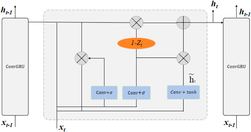
Figure 3. The ConvGRU model’s flowchart delineates its process.
The equations presented below outline the key components and operations of the ConvGRU model, elucidating its mechanism for processing sequential data. Each equation contributes to the understanding of how information flows through the model, culminating in the generation of output predictions.
Input Convolution: For each time step
where
Reset Gate: Controls the degree to which the previous hidden state
where
Update Gate: Regulates the amount of information from the previous hidden state
where
Candidate Hidden State: Represents the proposed new hidden state value at time step
where
Hidden State Update: Combines information from the previous hidden state and the candidate hidden state to generate the updated hidden state at time step
where
Layer Normalization: Layer normalization is applied to stabilize the training process and improve the model’s performance. It normalizes the hidden states across the feature dimension.
where
Output Computation: Computes the output at time step
where
In our model, the Convolutional Gated Recurrent Unit (ConvGRU) is applied to the task of predicting soil pollutants. By incorporating the ConvGRU model, we can effectively utilize the spatiotemporal information present in soil pollutant data. Through the combination of convolutional operations and gated mechanisms, the ConvGRU model enables precise prediction and assessment of soil pollutants. Specifically, the ConvGRU model excels in capturing the spatial distribution patterns and temporal trends within soil pollutant data. This enhances the model’s prediction accuracy and robustness, providing valuable technical support for soil environmental monitoring and management.
In conducting our deep learning experiments for this study, we selected four datasets:
The United States Environmental Protection Agency (EPA) dataset Mitra et al. (2023) provides extensive soil pollution datasets covering soil quality information nationwide. These datasets include concentrations of organic and inorganic compounds, heavy metal contents, volatile organic compounds (VOCs), and persistent organic pollutants (POPs), among others. EPA datasets typically contain detailed geographical coordinates, soil sampling information, and pollutant concentrations, which can be utilized for analyses of soil pollution distribution patterns, risk assessments, and environmental monitoring applications. The EPA dataset consists of approximately 10,000 sampling points, with each point providing concentrations for over 50 different pollutants. The dataset includes metadata such as sampling depth, soil type, and land use, which are essential for comprehensive soil quality analysis. These datasets serve as valuable references for researchers and policymakers to better understand soil pollution issues and develop corresponding management measures.
The SoilGrids dataset is a global soil property dataset Dinamarca et al. (2023) developed by the International Soil Reference and Information Centre (ISRIC). It provides spatially explicit information on various soil properties, including soil organic carbon content, pH, texture, and other key attributes, at different depths and resolutions. The dataset is generated through machine learning techniques and soil observations from various sources, offering valuable insights into soil variability and distribution patterns worldwide. SoilGrids facilitates a wide range of applications, such as soil mapping, environmental modeling, agricultural management, and land use planning. It covers different soil depths (0–5 cm, 5–15 cm, 15–30 cm, 30–60 cm, 60–100 cm, and 100–200 cm) with a spatial resolution of 250 m. The dataset is generated through machine learning techniques and soil observations from various sources, offering valuable insights into soil variability and distribution patterns worldwide. SoilGrids facilitates a wide range of applications, such as soil mapping, environmental modeling, agricultural management, and land use planning, contributing to improved soil management practices and sustainable land use strategies on a global scale.
The European Soil Data Centre (ESDAC) dataset Panagos et al. (2022) is a resource supported by the European Union (EU), aimed at providing comprehensive information about soils across Europe. This dataset contains soil sample data from various locations in Europe, covering key soil properties such as soil texture, soil type, organic carbon content, pH value, and more. These data are collected from diverse sources including ground observations, satellite remote sensing, field surveys, and soil monitoring projects in different countries and regions. The dataset includes detailed metadata for each sample point, such as geographical coordinates, sampling methods, and analysis techniques. These data are collected from diverse sources including ground observations, satellite remote sensing, field surveys, and soil monitoring projects in different countries and regions. The ESDAC dataset serves as a valuable resource of soil information for researchers, policymakers, and decision-makers, facilitating applications in soil management, environmental protection, agricultural production, and land planning.
The National Soil Inventory (NSI) dataset Prout et al. (2022) is a comprehensive collection of soil data compiled as part of a national-level soil survey initiative. It typically includes detailed information on soil properties, chemical composition, and contaminant concentrations from soil samples collected across various regions within a country. The NSI dataset encompasses data from thousands of sampling locations, providing extensive coverage of different soil types and land uses. It includes metadata such as sampling dates, depths, and methods, which are crucial for accurate analysis and interpretation. The NSI dataset serves as a valuable resource for soil research, environmental management, agricultural planning, and policy-making. It provides essential insights into soil quality, pollution levels, and spatial distribution patterns, supporting diverse applications in soil conservation, land use planning, and pollution mitigation efforts.
Step1: Data Preprocessing
Step2: Model Training
Before diving into model training, it is essential to meticulously configure network parameters, design an optimal architecture, and implement an effective training process.
Network Parameter Settings: Setting the parameters of the neural network architecture is crucial for effective model training. We configured parameters such as the learning rate, batch size, and number of epochs. We set the learning rate to 0.001, the batch size to 32, and conducted training for 100 epochs to optimize the model’s performance.
Model Architecture Design: Designing the architecture of the neural network involves determining the number of layers, types of activation functions, and the size of hidden units. We designed a deep learning architecture with three convolutional layers followed by two GRU layers, each with a ReLU activation function. The convolutional layers had 64, 128, and 256 filters, respectively, while the GRU layers had 128 hidden units.
Model Training Process: The model training process involves feeding the preprocessed data into the neural network and iteratively updating the model parameters to minimize the loss function. We utilized the Adam optimizer with a categorical cross-entropy loss function to train the model. The training process involved forward and backward propagation of data batches through the network, adjusting the weights and biases using gradient descent. We monitored the training progress by evaluating the model’s performance on the validation set after each epoch, ensuring convergence and preventing overfitting.
Algorithm 1 outlines the algorithmic process for training the SSA based attention-ConvGRU network.
Algorithm 1.Training procedure for SSA based attention-ConvGRU network.
Data: EPA dataset, SoilGrids dataset, ESDAC dataset, NSI dataset
Result: Trained SSA based attention-ConvGRU network
Initialize network parameters: learning rate, batch size, number of epochs;
for each epoch do
for each mini-batch in training data do
Perform data augmentation if necessary;
Forward pass through the network to compute predicted outputs;
Compute loss function using predicted outputs and ground truth labels;
Backpropagate gradients through the network;
Update network weights using optimization algorithm (e.g., Adam);
end
Evaluate model performance on validation set using MAE, RMSE, etc.,;
if early stopping criterion is met then
break;
end
end
Step3: Model Evaluation
where:
where:
where:
In Table 2, it is evident that our model outperforms other benchmark models across various datasets, showcasing its notable superiority in performance. On the EPA dataset, our model achieves an average absolute error (MAE) of 11.01, a root mean square error (RMSE) of 13.77, and an average absolute percentage error (MAPE) of 27.62. Compared to other models such as ARIMA-WOA-LSTM and CNN-BiLSTM, our model reduces MAE and RMSE by over 45% and 50% respectively. This significant reduction can be attributed to the enhanced ability of our model to capture complex spatiotemporal dependencies through the integration of the attention mechanism and ConvGRU, as well as the optimization provided by SSA. Our model’s remarkable enhancement is further evident in other datasets. For instance, on the SoilGrids dataset, our model achieves an MAE of 12.29 and an RMSE of 20.46, marking an improvement of at least 15% and 10%, respectively, compared to other models. The improvement in SoilGrids dataset performance highlights the robustness of our model in handling high-resolution global soil data, benefiting from the effective feature extraction and sequence modeling capabilities of ConvGRU combined with the selective focus of the attention mechanism. On the ESDAC dataset, although all models show similar performance in terms of MAPE, our model still demonstrates superior performance in MAE and RMSE, with values of 13.25 and 13.96 respectively, significantly lower than other models. Similarly, on the NSI dataset, our model achieves MAE and RMSE of 16.91 and 17.65 respectively, indicating significant advantages in prediction accuracy and stability. The lower error rates on the NSI dataset suggest that our model is highly effective in managing national-level soil data, which often involves diverse soil types and contamination levels. The adaptability of our model to various scales and types of data is a testament to the robust framework of SSA optimization and the attention-ConvGRU combination. Overall, these results not only validate the efficiency of our model in managing diverse types and scales of datasets but also highlight the adaptability and superiority of the SSA optimization and attention-ConvGRU combination. For soil pollutant prediction tasks, this model architecture evidently provides a more precise and reliable approach. The integration of SSA helps in fine-tuning the model parameters for optimal performance, while the attention mechanism ensures that the model focuses on the most relevant features within the data, enhancing its predictive capabilities. Figure 4 visually depicts the table contents, further showcasing the outstanding performance of our model across various datasets, aiding in the intuitive understanding of performance differences across different metrics.
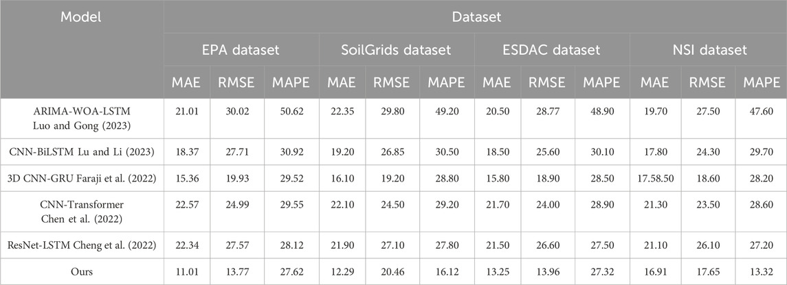
Table 2. Comparison of MAE, RMSE, and MAPE across different datasets and models.
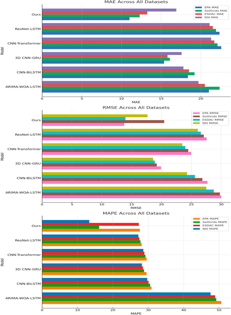
Figure 4. Comparison of MAE, RMSE, and MAPE across different datasets and models.
As depicted in Table 3, our model outperforms existing techniques across various datasets. Specifically, on the EPA dataset, our model comprises only 119.71 million parameters and 164.14 billion floating-point operations (Flops), significantly lower than ARIMA-WOA-LSTM’s 244.11 million parameters and 244.94 billion Flops, as well as CNN-BiLSTM’s 302.01 million parameters and 232.96 billion Flops. In terms of inference time and training time, our model requires only 110.01 milliseconds and 149.93 s respectively, reducing the inference time by over 60% compared to the ARIMA-WOA-LSTM model and halving the training time. On the SoilGrids dataset, our model also performs admirably, with 110.66 million parameters and 155.1 billion Flops, while 3D CNN-GRU has 371.48 million parameters and 332.89 billion Flops. Additionally, our model significantly reduces both inference and training times. For the ESDAC dataset, our model achieves efficient inference (170.7 milliseconds) and training (228.63 s) with lower parameter count (140.04 million) and computational load (149.32 billion Flops). On the NSI dataset, our model not only maintains low parameter count (212.11 million) and computational load (197.37 billion Flops) but also leads significantly in inference time (186.9 milliseconds) and training time (194.2 s) compared to other models, such as CNN-Transformer, which requires 336.42 s for training. Overall, our model not only demonstrates significant advantages in parameter efficiency and computational efficiency but also exhibits significantly faster execution speeds than other methods, proving the practicality and efficiency of our model. Figure 5 visualizes the table contents, providing a more intuitive demonstration of our model’s significant advantages in computational resources and performance. These graphical representations facilitate easier understanding and communication of the results analysis.
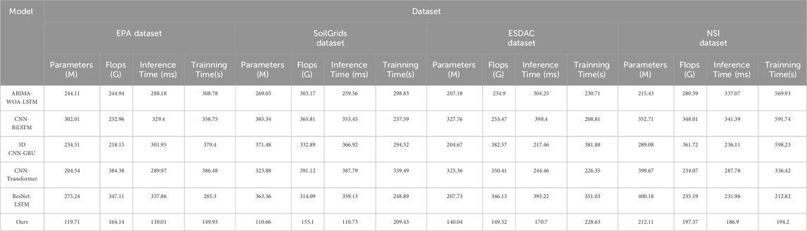
Table 3. Comparison of model performance metrics and computational efficiency across datasets and models.
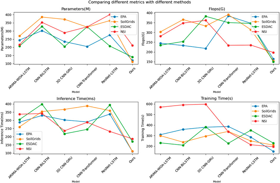
Figure 5. Comparison of model performance metrics and computational efficiency across datasets and models.
As illustrated in Table 4, our model achieved superior performance in predicting various types of soil pollutants in the EPA dataset. Specifically, our model excelled in predicting lead (Pb) and polycyclic aromatic hydrocarbons (PAHs), with RMSE values of 16.01 and 12.29, respectively, significantly outperforming other models. In the prediction of copper (Cu) and pollutants with carbon chain lengths of
Table 4. Comparison of RMSE of pollutant predictions by different models under the EPA dataset.
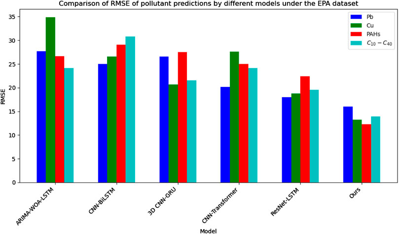
Figure 6. Comparison of RMSE of pollutant predictions by different models under the EPA dataset.
In Table 4, our model shows the performance in predicting various soil pollutants, especially lead (Pb), copper (Cu), polycyclic aromatic hydrocarbons (PAHs), and
As shown in Table 5, the ablation study results reveal that each component (SSA optimization, Attention mechanism, and ConvGRU) significantly contributes to the model’s performance. Specifically, the full model achieves the lowest errors across all datasets. For instance, on the EPA dataset, the full model achieves an MAE of 11.01 and an RMSE of 13.77. Removing SSA optimization increases the MAE to 14.85 and the RMSE to 23.89. Similarly, removing the Attention mechanism leads to an MAE of 15.62 and an RMSE of 25.13. The most significant degradation occurs when ConvGRU is removed, resulting in an MAE of 16.34 and an RMSE of 26.47. This trend is consistent across the other datasets as well. On the SoilGrids dataset, the full model outperforms all ablated versions, with noticeable increases in error metrics when any component is removed. Specifically, removing SSA optimization, Attention mechanism, and ConvGRU results in MAE increases to 13.92, 14.45, and 15.15, respectively, and RMSE increases to 21.34, 21.78, and 22.89. For the ESDAC dataset, the full model again shows the best performance, with removing SSA optimization, Attention mechanism, and ConvGRU leading to MAE increases to 14.97, 15.54, and 16.28, and RMSE increases to 21.89, 22.67, and 23.56, respectively. On the NSI dataset, removing SSA optimization, Attention mechanism, and ConvGRU results in MAE increases to 17.01, 18.21, and 18.32, and RMSE increases to 24.78, 25.43, and 26.89, respectively. These results validate the effectiveness and necessity of each component in the SSA-optimized Attention-ConvGRU model. SSA optimization significantly enhances the model’s parameter optimization efficiency and predictive accuracy, as evidenced by the substantial error increases upon its removal. The Attention mechanism plays a crucial role in capturing important spatiotemporal features, and its absence leads to notable performance degradation. ConvGRU is essential for handling complex spatiotemporal data, with its removal causing the most significant drop in performance, highlighting its importance in integrating spatiotemporal features for accurate and stable predictions.
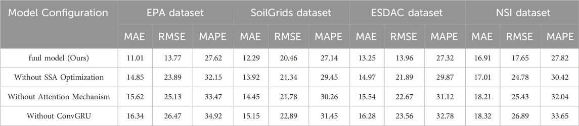
Table 5. Ablation experiment of SSA-optimized Attention-ConvGRU model.
The full model consistently outperforms its ablated versions, confirming that the combination of SSA optimization, Attention mechanism, and ConvGRU is critical for achieving high predictive performance. This comprehensive analysis underscores the robustness and superiority of our proposed model in predicting soil pollutants. Figure 7 visualizes the table content, further illustrating the impact of each component on the model’s performance.
Figure 7. Ablation experiment of ConvGRU module.
In this study, we proposed an SSA-optimized Attention-ConvGRU model for predicting soil contaminants and assessing risk. Although experimental results demonstrated that this model significantly outperforms traditional methods and other deep learning models across multiple datasets, we recognize several limitations and areas for potential improvement.
One limitation is that while the SSA algorithm effectively optimizes model parameters, the model’s convergence speed and prediction accuracy need further enhancement when dealing with highly nonlinear and high-dimensional data. Future research could explore the integration of other optimization algorithms, such as Genetic Algorithms (GA) or Particle Swarm Optimization (PSO), to further improve optimization efficiency and predictive performance. Additionally, the model’s computational resource consumption is relatively high, particularly when processing large-scale data. This could limit its application in resource-constrained environments. Future studies might investigate more efficient computational methods or model compression techniques, such as pruning and quantization, to reduce computational costs and accelerate prediction speed. Moreover, although our model exhibits strong adaptability across various types and scales of datasets, its generalizability requires further validation. Future research could incorporate more diverse soil pollution data and cross-regional validation to enhance the model’s adaptability and accuracy under different environmental conditions. Finally, while this study primarily focuses on predicting soil contaminants, the complexity of soil environments necessitates considering other relevant factors, such as soil moisture, temperature, and vegetation cover. Future research could explore multimodal data fusion techniques to incorporate more environmental factors into the model, providing a more comprehensive and accurate assessment of soil pollution.
This study introduced and validated an SSA-optimized Attention-ConvGRU model aimed at improving the accuracy and stability of soil contaminant prediction and risk assessment. Experimental results indicated that the proposed model performs exceptionally well across multiple datasets, significantly surpassing traditional methods and other deep learning models. Specifically, the SSA algorithm effectively optimized model parameters, and the integration of the attention mechanism with ConvGRU significantly enhanced the model’s ability to handle complex spatiotemporal data, leading to more accurate predictions of soil contaminant distribution and trends. The primary contributions of this research include the development of a novel model architecture that combines SSA, attention mechanisms, and ConvGRU, which markedly improves the accuracy and stability of soil contaminant predictions. Additionally, the model’s superior performance was validated across multiple datasets, demonstrating its robustness and adaptability to different types and scales of soil data. Despite the significant advancements achieved, this study acknowledges certain limitations. Future research will focus on enhancing the model’s convergence speed and prediction accuracy, reducing computational resource consumption, improving generalizability, and incorporating additional environmental factors for a more comprehensive soil pollution assessment.
In summary, this research demonstrates the substantial potential of deep learning technology in the field of soil pollution prediction, offering new technological pathways and theoretical support for environmental monitoring and pollution control. We believe that with continuous improvement and optimization, this research direction will have broad application prospects and significant practical implications.
The original contributions presented in the study are included in the article/Supplementary Material, further inquiries can be directed to the corresponding author.
YL: Data curation, Formal Analysis, Investigation, Resources, Writing–original draft. JZ: Investigation, Resources, Validation, Writing–review and editing. YZ: Software, Supervision, Validation, Visualization, Writing–review and editing. JL: Investigation, Methodology, Project administration, Resources, Writing–original draft. JD: Data curation, Formal Analysis, Funding acquisition, Investigation, Writing–review and editing. CJ: Conceptualization, Data curation, Formal Analysis, Funding acquisition, Writing–original draft. JJ: Formal Analysis, Funding acquisition, Software, Supervision, Writing–original draft. DW: Investigation, Methodology, Project administration, Resources, Writing–original draft.
The author(s) declare that financial support was received for the research, authorship, and/or publication of this article. This work was sponsored in part by Science and Technology Project of Hebei Education Department (BJK2022058). Science and Technology Support Plan of Qinhuangdao Science and Technology Bureau (202301A168). Doctoral Foundation of Hebei University of Environmental Engineering (2023BSJJ05). Science and Technology Project of Hebei Education Department (ZD2021038).
JL was employed by Central Control Technology (Xi’an) Co., Ltd.
The remaining authors declare that the research was conducted in the absence of any commercial or financial relationships that could be construed as a potential conflict of interest.
All claims expressed in this article are solely those of the authors and do not necessarily represent those of their affiliated organizations, or those of the publisher, the editors, and the reviewers. Any product that may be evaluated in this article, or claim that may be made by its manufacturer, is not guaranteed or endorsed by the publisher.
Awadallah, M. A., Al-Betar, M. A., Doush, I. A., Makhadmeh, S. N., and Al-Naymat, G. (2023). Recent versions and applications of sparrow search algorithm. Archives Comput. Methods Eng. 30, 2831–2858. doi:10.1007/s11831-023-09887-z
Baragaño, D., Ratié, G., Sierra, C., Chrastnỳ, V., Komárek, M., and Gallego, J. (2022). Multiple pollution sources unravelled by environmental forensics techniques and multivariate statistics. J. Hazard. Mater. 424, 127413. doi:10.1016/j.jhazmat.2021.127413
Bijitha, C., and Nath, H. V. (2022). On the effectiveness of image processing based malware detection techniques. Cybern. Syst. 53, 615–640. doi:10.1080/01969722.2021.2020471
Chelabi, H., Khadir, M. T., Chikhaoui, B., and Telmoudi, A. J. (2022). Comparison of deep learning architectures for short-term electrical load forecasting based on multi-modal data. Cybern. Syst. 53, 186–207. doi:10.1080/01969722.2021.2008679
Chen, Y., Chen, X., Xu, A., Sun, Q., and Peng, X. (2022). A hybrid cnn-transformer model for ozone concentration prediction. Air Qual. Atmos. Health 15, 1533–1546. doi:10.1007/s11869-022-01197-w
Cheng, X., Zhang, W., Wenzel, A., and Chen, J. (2022). Stacked resnet-lstm and coral model for multi-site air quality prediction. Neural Comput. Appl. 34, 13849–13866. doi:10.1007/s00521-022-07175-8
Cui, S., Gao, Y., Huang, Y., Shen, L., Zhao, Q., Pan, Y., et al. (2023). Advances and applications of machine learning and deep learning in environmental ecology and health. Environ. Pollut. 122358. doi:10.1016/j.envpol.2023.122358
Dinamarca, D. I., Galleguillos, M., Seguel, O., and Faúndez Urbina, C. (2023). Clsoilmaps: a national soil gridded database of physical and hydraulic soil properties for Chile. Sci. Data 10, 630. doi:10.1038/s41597-023-02536-x
Duan, C., Wang, B., and Li, J. (2022). Prediction model of soil heavy metal content based on particle swarm algorithm optimized neural network. Comput. Intell. Neurosci. 2022, 1–10. doi:10.1155/2022/9693175
Faraji, M., Nadi, S., Ghaffarpasand, O., Homayoni, S., and Downey, K. (2022). An integrated 3d cnn-gru deep learning method for short-term prediction of pm2. 5 concentration in urban environment. Sci. Total Environ. 834, 155324. doi:10.1016/j.scitotenv.2022.155324
Gao, B., Stein, A., and Wang, J. (2022). A two-point machine learning method for the spatial prediction of soil pollution. Int. J. Appl. Earth Observation Geoinformation 108, 102742. doi:10.1016/j.jag.2022.102742
Gautam, K., Sharma, P., Dwivedi, S., Singh, A., Gaur, V. K., Varjani, S., et al. (2023). A review on control and abatement of soil pollution by heavy metals: emphasis on artificial intelligence in recovery of contaminated soil. Environ. Res. 225, 115592. doi:10.1016/j.envres.2023.115592
Gharehchopogh, F. S., Namazi, M., Ebrahimi, L., and Abdollahzadeh, B. (2023). Advances in sparrow search algorithm: a comprehensive survey. Archives Comput. Methods Eng. 30, 427–455. doi:10.1007/s11831-022-09804-w
Gonzalez, J., Yu, W., and Telesca, L. (2022). Gated recurrent units based recurrent neural network for forecasting the characteristics of the next earthquake. Cybern. Syst. 53, 209–222. doi:10.1080/01969722.2021.1981637
Guo, M.-H., Xu, T.-X., Liu, J.-J., Liu, Z.-N., Jiang, P.-T., Mu, T.-J., et al. (2022). Attention mechanisms in computer vision: a survey. Comput. Vis. media 8, 331–368. doi:10.1007/s41095-022-0271-y
Janga, J. K., Reddy, K. R., and Kvns, R. (2023). Integrating artificial intelligence, machine learning, and deep learning approaches into remediation of contaminated sites: a review. Chemosphere 345, 140476. doi:10.1016/j.chemosphere.2023.140476
Jiang, Y., Li, C., Song, H., and Wang, W. (2022). Deep learning model based on urban multi-source data for predicting heavy metals (cu, zn, ni, cr) in industrial sewer networks. J. Hazard. Mater. 432, 128732. doi:10.1016/j.jhazmat.2022.128732
Khan, J., Singh, R., Upreti, P., and Yadav, R. K. (2022). Geo-statistical assessment of soil quality and identification of heavy metal contamination using integrated gis and multivariate statistical analysis in industrial region of western India. Environ. Technol. Innovation 28, 102646. doi:10.1016/j.eti.2022.102646
Li, P., Hao, H., Bai, Y., Li, Y., Mao, X., Xu, J., et al. (2022). Convolutional neural networks-based health risk modelling of some heavy metals in a soil-rice system. Sci. Total Environ. 838, 156466. doi:10.1016/j.scitotenv.2022.156466
Liu, C., Li, H., Xu, J., Gao, W., Shen, X., and Miao, S. (2023a). Applying convolutional neural network to predict soil erosion: a case study of coastal areas. Int. J. Environ. Res. Public Health 20, 2513. doi:10.3390/ijerph20032513
Liu, J., Kang, H., Tao, W., Li, H., He, D., Ma, L., et al. (2023b). A spatial distribution–principal component analysis (sd-pca) model to assess pollution of heavy metals in soil. Sci. Total Environ. 859, 160112. doi:10.1016/j.scitotenv.2022.160112
Liu, Z., Fei, Y., Shi, H., Mo, L., and Qi, J. (2022). Prediction of high-risk areas of soil heavy metal pollution with multiple factors on a large scale in industrial agglomeration areas. Sci. Total Environ. 808, 151874. doi:10.1016/j.scitotenv.2021.151874
Lu, Y., and Li, K. (2023). Multistation collaborative prediction of air pollutants based on the cnn-bilstm model. Environ. Sci. Pollut. Res. 30, 92417–92435. doi:10.1007/s11356-023-28877-z
Luo, J., and Gong, Y. (2023). Air pollutant prediction based on arima-woa-lstm model. Atmos. Pollut. Res. 14, 101761. doi:10.1016/j.apr.2023.101761
Mei, P., Li, M., Zhang, Q., Li, G., and song, L. (2022). Prediction model of drinking water source quality with potential industrial-agricultural pollution based on cnn-gru-attention. J. Hydrology 610, 127934. doi:10.1016/j.jhydrol.2022.127934
Mirzavand Borujeni, S., Arras, L., Srinivasan, V., and Samek, W. (2023). Explainable sequence-to-sequence gru neural network for pollution forecasting. Sci. Rep. 13, 9940. doi:10.1038/s41598-023-35963-2
Mitra, S., Young, M., Breidt, J., Pallickara, S., and Pallickara, S. (2023). “Rubiks: rapid explorations and summarization over high dimensional spatiotemporal datasets,” in Proceedings of the IEEE/ACM 10th international conference on big data computing, applications and technologies, 1–11.
Nadiri, A. A., Moazamnia, M., Sadeghfam, S., Gnanachandrasamy, G., and Venkatramanan, S. (2022). Formulating convolutional neural network for mapping total aquifer vulnerability to pollution. Environ. Pollut. 304, 119208. doi:10.1016/j.envpol.2022.119208
Panagos, P., Van Liedekerke, M., Borrelli, P., Köninger, J., Ballabio, C., Orgiazzi, A., et al. (2022). European soil data centre 2.0: soil data and knowledge in support of the eu policies. Eur. J. Soil Sci. 73, e13315. doi:10.1111/ejss.13315
Pisal, P. S., and Vidyarthi, A. (2023). Adaptive aquila optimization controlled deep convolutional neural network for power management in supercapacitors/battery of electric vehicles. Cybern. Syst. 54, 1062–1085. doi:10.1080/01969722.2022.2157606
Prout, J. M., Shepherd, K. D., McGrath, S. P., Kirk, G. J., Hassall, K. L., and Haefele, S. M. (2022). Changes in organic carbon to clay ratios in different soils and land uses in england and wales over time. Sci. Rep. 12, 5162. doi:10.1038/s41598-022-09101-3
Raimi, M. O., Iyingiala, A.-A., Sawyerr, O. H., Saliu, A. O., Ebuete, A. W., Emberru, R. E., et al. (2022). “Leaving no one behind: impact of soil pollution on biodiversity in the global south: a global call for action,” in Biodiversity in Africa: potentials, threats and conservation (Springer), 205–237.
Ren, B., and Wang, Z. (2024). Strategic priorities, tasks, and pathways for advancing new productivity in the Chinese-style modernization. J. Xi’an Univ. Finance Econ. 37, 3–11. doi:10.19331/j.cnki.jxufe.20240008.002
Shin, J., Yu, J., Wang, L., Seo, J., Huynh, H. H., and Jeong, G. (2023). Spectral indices to assess pollution level in soils: case-adaptive and universal detection models for multiple heavy metal pollution under laboratory conditions. IEEE Trans. Geoscience Remote Sens. 61, 1–16. doi:10.1109/tgrs.2023.3297126
Siddthan, R., and Shanthi, P. (2022). “A comprehensive survey on cnn models on assessment of nitrate contamination in groundwater,” in 2022 6th international Conference on electronics, Communication and aerospace technology (IEEE), 1250–1254.
Tao, H., Liao, X., Cao, H., Zhao, D., and Hou, Y. (2022). Three-dimensional delineation of soil pollutants at contaminated sites: progress and prospects. J. Geogr. Sci. 32, 1615–1634. doi:10.1007/s11442-022-2013-6
Wang, J., Li, F., An, Y., Zhang, X., and Sun, H. (2024). Toward robust LiDAR-camera fusion in BEV space via mutual deformable attention and temporal aggregation. IEEE Trans. Circuits Syst. Video Technol. 34, 5753–5764. doi:10.1109/tcsvt.2024.3366664
Wang, X., Wang, L., Zhang, Q., Liang, T., Li, J., Hansen, H. C. B., et al. (2022). Integrated assessment of the impact of land use types on soil pollution by potentially toxic elements and the associated ecological and human health risk. Environ. Pollut. 299, 118911. doi:10.1016/j.envpol.2022.118911
Wu, C., Chao, Y., Shu, L., and Qiu, R. (2022). Interactions between soil protists and pollutants: an unsolved puzzle. J. Hazard. Mater. 429, 128297. doi:10.1016/j.jhazmat.2022.128297
Xu, H., and Zhang, C. (2023). Development and applications of gis-based spatial analysis in environmental geochemistry in the big data era. Environ. Geochem. Health 45, 1079–1090. doi:10.1007/s10653-021-01183-8
Yao, Y., and Liu, Z. (2024). The new development concept helps accelerate the formation of new quality productivity: theoretical logic and implementation paths. J. Xi’an Univ. Finance Econ. 37, 3–14. doi:10.19331/j.cnki.jxufe.20240202.002
Zeng, W., Wan, X., Lei, M., Gu, G., and Chen, T. (2022). Influencing factors and prediction of arsenic concentration in pteris vittata: a combination of geodetector and empirical models. Environ. Pollut. 292, 118240. doi:10.1016/j.envpol.2021.118240
Zhang, H., Wang, C., Tian, S., Lu, B., Zhang, L., Ning, X., et al. (2023). Deep learning-based 3d point cloud classification: a systematic survey and outlook. Displays 79, 102456. doi:10.1016/j.displa.2023.102456
Zhao, W., Ma, J., Liu, Q., Dou, L., Qu, Y., Shi, H., et al. (2023). Accurate prediction of soil heavy metal pollution using an improved machine learning method: a case study in the pearl river delta, China. Environ. Sci. Technol. 57, 17751–17761. doi:10.1021/acs.est.2c07561
Zheng, S., Wang, J., Zhuo, Y., Yang, D., and Liu, R. (2022). Spatial distribution model of dehp contamination categories in soil based on bi-lstm and sparse sampling. Ecotoxicol. Environ. Saf. 229, 113092. doi:10.1016/j.ecoenv.2021.113092
Keywords: soil pollution, deep learning, sparrow search algorithm, ConvGRU, attention mechanisms, attention-ConvGRU
Citation: Liang Y, Zhao J, Zhang Y, Li J, Ding J, Jing C, Ji J and Wu D (2024) Developing an SSA-optimized attention-ConvGRU model for predicting and assessing soil contaminant distribution. Front. Environ. Sci. 12:1440296. doi: 10.3389/fenvs.2024.1440296
Received: 29 May 2024; Accepted: 15 July 2024;
Published: 08 August 2024.
Edited by:
Arindam Malakar, University of Nebraska-Lincoln, United StatesReviewed by:
Alakananda Mitra, University of Nebraska-Lincoln, United StatesCopyright © 2024 Liang, Zhao, Zhang, Li, Ding, Jing, Ji and Wu. This is an open-access article distributed under the terms of the Creative Commons Attribution License (CC BY). The use, distribution or reproduction in other forums is permitted, provided the original author(s) and the copyright owner(s) are credited and that the original publication in this journal is cited, in accordance with accepted academic practice. No use, distribution or reproduction is permitted which does not comply with these terms.
*Correspondence: Yajie Liang, bGlhbmd5YWppZTIwMjQwNEAxNjMuY29t
Disclaimer: All claims expressed in this article are solely those of the authors and do not necessarily represent those of their affiliated organizations, or those of the publisher, the editors and the reviewers. Any product that may be evaluated in this article or claim that may be made by its manufacturer is not guaranteed or endorsed by the publisher.
Research integrity at Frontiers
Learn more about the work of our research integrity team to safeguard the quality of each article we publish.