Estimation of water quality in Korattur Lake, Chennai, India, using Bayesian optimization and machine learning

Assessing water quality becomes imperative to facilitate informed decision-making concerning the availability and accessibility of water resources in Korattur Lake, Chennai, India, which has been adversely affected by human actions. Although numerous state-of-the-art studies have made significant advancements in water quality classification, conventional methods for training machine learning model parameters still require substantial human and material resources. Hence, this study employs stochastic gradient descent (SGD), adaptive boosting (AdaBoosting), Perceptron, and artificial neural network algorithms to classify water quality categories as these well-established methods, combined with Bayesian optimization for hyperparameter tuning, provide a robust framework to demonstrate significant performance enhancements in water quality classification. The input features for model training from 2010 to 2019 comprise water parameters such as pH, phosphate, total dissolved solids (TDS), turbidity, nitrate, iron, chlorides, sodium, and chemical oxygen demand (COD). Bayesian optimization is employed to dynamically tune the hyperparameters of different machine learning algorithms and select the optimal algorithms with the best performance. Comparing the performance of different algorithms, AdaBoosting exhibits the highest performance in water quality level classification, as indicated by its superior accuracy (100%), precision (100%), recall (100%), and F1 score (100%). The top four important factors for water quality level classification are COD (0.684), phosphate (0.119), iron (0.112), and TDS (0.084). Additionally, variations or changes in phosphate levels are likely to coincide with similar variations in TDS levels.

1 Introduction

Ensuring water quality is a critical environmental challenge worldwide. The accurate assessment and management of water quality are essential for safeguarding public health, preserving ecosystems, and supporting sustainable development (Uddin et al., 2024b). Traditional methods, such as the water quality index (WQI), provide useful metrics for assessing water quality but have limitations, including a simplified approach, subjective parameter selection, and a lack of consideration for specific pollutants and health risks (Bhateria and Jain, 2016; Shams et al., 2023). Complementary approaches and a broader understanding of water quality are necessary for a comprehensive and accurate evaluation (Uddin et al., 2023b; Chen et al., 2023; Ehteram et al., 2024).

In recent years, machine learning has gained significant attention in the environmental field due to its capacity to extract underlying patterns from vast amounts of data (Lin et al., 2022a; Granata et al., 2024). Machine learning techniques have been introduced to predict various WQI values, leveraging their ability to address nonlinear regression and classification challenges (Shams et al., 2023; Yan et al., 2023). Several approaches, such as the adaptive neuro-fuzzy inference system (ANFIS), radial basis function neural network (RBF-ANN), and multi-layer perceptron neural network (MLP-ANN), have been employed to forecast water quality in different contexts (Najah Ahmed et al., 2019). However, there is still room for improvement, particularly in terms of considering additional relevant parameters and optimizing the model performance (Ahmed et al., 2019).

One significant challenge in machine learning applications is the efficient tuning of the model parameters. Traditional methods such as grid search and random search are often resource-intensive (Lin et al., 2022a). For instance, in the context of water quality prediction, researchers have applied 16 novel hybrid data-mining algorithms and conducted a series of experiments to optimize the models (Bui et al., 2020). Lin et al. also confronted this problem when using machine learning to estimate the amount of municipal solid waste (Lin et al., 2021). Fortunately, the method of grid search, random search, and Bayesian optimization can effectively solve this problem. Bayesian optimization offers higher efficiency, a better exploration–exploitation balance, adaptability, and suitability for high-dimensional parameter spaces compared to grid search and random search in machine learning parameter optimization (González and Zavala, 2023; Zhu et al., 2024). In addition, despite these advancements, the interpretability of machine learning models remains a significant challenge, especially in complex environmental applications (Lin et al., 2022a).

Given these considerations, our study addresses the gap by employing machine learning models optimized through Bayesian optimization to classify the water quality categories in Korattur Lake, Chennai. Specifically, stochastic gradient descent (SGD), adaptive boosting (AdaBoosting), Perceptron, and artificial neural network (ANN) algorithms are utilized. Water parameters such as pH, phosphate (P), total dissolved solids (TDS), turbidity, nitrate, iron, chlorides, sodium, and chemical oxygen demand (COD) were selected as input features for the model training from 2010 to 2019. The performance of the models is evaluated using metrics such as confusion matrix, accuracy, precision, and the F1 score. In addition, the important features from the best models were visualized to provide valuable references for the efficient prediction of future water quality levels and preservation of the overall environmental health of Korattur Lake.

Although this study focuses on Korattur Lake in Chennai, India, the methodology and findings have broader implications. The integration of Bayesian optimization with machine learning can be applied to other water bodies worldwide, enhancing water quality assessment and management practices globally. This approach provides a robust framework for environmental scientists and policymakers to develop more effective water management strategies, ensuring the sustainable use and conservation of vital water resources.

2 Materials and methods

2.1 Data collection

The dataset was collected from the open-source dataset (https://github.com/JahnaviSrividya/Korattur-Lake-Water-Quality-Dataset). This dataset consists of nine pollution indicators, pH, P, TDS, turbidity, nitrate, iron, chlorides, sodium, and COD, and more than 5,000 records from 2010 to 2019. Figure 1 shows the distribution of various indicators.

Figure 1

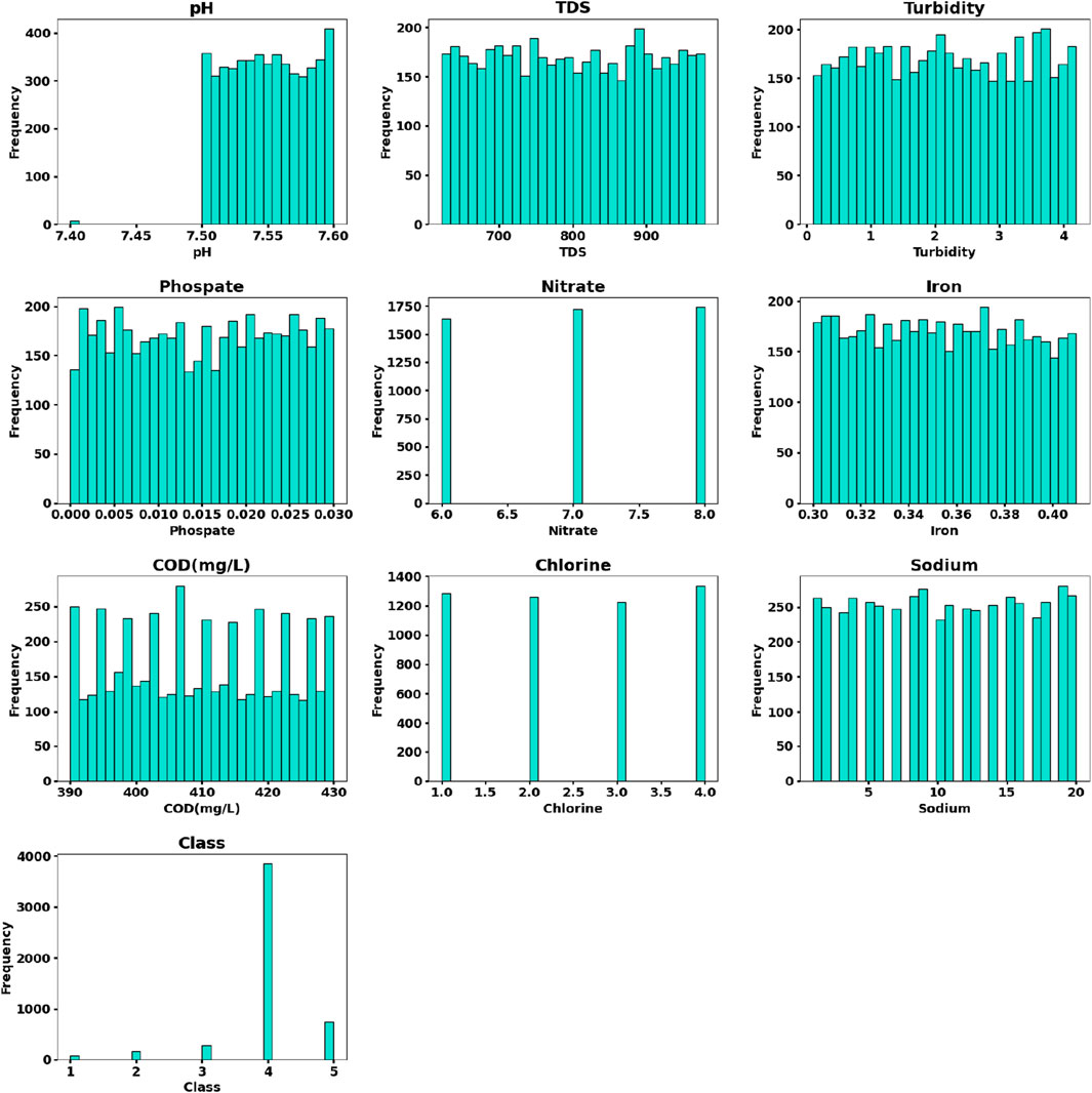
Figure 1. Distribution of various pollution indicators in the dataset.

2.2 Water quality level

The water quality level Q_i for the ith parameter can be calculated using Eq. 2–1:

${\mathrm{Q}}_{\mathrm{i}}=\frac{\left({\mathrm{V}}_{\mathrm{i}}-{\mathrm{V}}_{\mathrm{i}0}\right)}{\left({\mathrm{S}}_{\mathrm{i}}-{\mathrm{V}}_{\mathrm{i}0}\right)}\times 100,(\mathrm{2–1})$

where $V_i$, $S_i$, and $V_{i0}$ represented the estimated value of the nth parameter, the desirable or permissible range, and the ideal value of the nth parameter in pure water. All ideal values are taken as zero, except pH = 7.0.

WQI can be calculated as the following Eq. 2-2:

$\text{WQI}=\frac{\sum \left({\mathrm{W}}_{\mathrm{i}}\times {\mathrm{Q}}_{\mathrm{i}}\right)}{{\displaystyle {\sum }_{\mathrm{i}=1}^9}{\mathrm{W}}_{\mathrm{i}}},(\mathrm{2–2})$

where ${\mathrm{W}}_{\mathrm{i}}$ is the weight allocated to each parameter; Q_i is the quality index of each parameter, which is calculated using Eq. 2–1.

Based on the WQI, the classes are classified as shown in Table 1.

Table 1

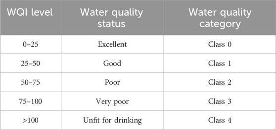
Table 1. Quality of water based on WQI.

2.3 Machine learning model

2.3.1 SGD

Taylor discovered that any function can be expressed as a polynomial in terms of its Nth order derivatives, as the following Eq. 2-3:

$\mathrm{f}\left(x\right)={\sum }_{n=0}^N\frac{f^{\left(n\right)}\left(a\right)}{n!}{\left(x-a\right)}^n+R_n\left(x\right).(\mathrm{2–3})$

Therefore, for any function that is (n + 1)-times differentiable, it can be approximated near a point (denoted as x₀) by the following Eq. 2-4:

$\mathrm{f}\left(x\right)=f\left(x_0\right)+f^{\prime }\left(x_0\right)\left(x-x_0\right)+\frac{f^{″}\left(x_0\right)}{2!}{\left(x-x_0\right)}^2+\dots +\frac{f^n\left(x_0\right)}{n!}{\left(x-x_0\right)}^n.(\mathrm{2–4})$

The Taylor series can be expanded to the first-order as the following Eq. 2-5:

$\mathrm{f}\left(x\right)\approx f\left(x_0\right)+f^{\prime }\left(x_0\right)\left(x-x_0\right).(\mathrm{2–5})$

In the context of gradient descent, the first-order expansion can be expressed as follows Eq. 2-6:

$\mathrm{J}\left(\theta \right)\approx J\left({\theta }_0\right)+f^{\prime }\left({\theta }_0\right)\left(\theta -{\theta }_0\right).(\mathrm{2–6})$

The essence of gradient descent can be summarized that it approximates the loss function through a first-order Taylor expansion and then seeks the minimum value of this approximation (Andrychowicz et al., 2016). The minimum value is considered the next iteration value for the iterative process.

2.3.2 AdaBoosting

AdaBoost is a prominent ensemble learning method renowned for its capability to create a robust classifier by effectively combining multiple weak classifiers (RATSCH et al., 2001; Belghit et al., 2023). When applied to the task of water quality level classification, AdaBoost begins with the preparation of a labeled dataset consisting of input features and corresponding multi-class labels specifically encoded for the prediction of water quality levels. In the initialization phase, equal weights are assigned to all samples within the training set, setting the foundation for the subsequent steps.

The AdaBoost iterations commence by training weak classifiers, evaluating their performance, updating sample weights, and constructing a weighted combination. This iterative process continues by training additional weak classifiers, wherein subsequent classifiers primarily focus on samples that were misclassified or possess higher weights. The ultimate culmination involves the fusion of these trained weak classifiers into a potent ensemble classifier utilizing a weighted voting scheme. The influence of each weak classifier in the final classification decision is determined by the assigned weights.

The trained AdaBoost model effectively predicts the labels of new, unseen data by aggregating the predictions of individual weak classifiers based on their assigned weights. AdaBoost iteratively enhances classification performance by assigning higher weights to challenging samples and leveraging the knowledge gained from errors made by previous weak classifiers. This iterative process empowers the ensemble model to proficiently tackle complex multi-class classification tasks by prioritizing the difficult instances.

It is noteworthy that AdaBoost can be deployed alongside diverse weak classifiers, and the number of iterations and the weighting scheme can be tailored to suit the characteristics of the dataset and performance evaluation. The strength of AdaBoost lies in its ability to harness the strengths of weak classifiers, allowing them to synergistically form a powerful and accurate classifier.

2.3.3 Perceptron

Figure 2 illustrates the structure of the Perceptron algorithm utilized for predicting water quality levels based on nine water quality indicators. It is essential to acknowledge that the Perceptron algorithm functions as a simple linear binary classifier and may not directly support multi-class classification (Zhang et al., 2023). To address this limitation, the one-vs-all strategy is employed, wherein multiple perceptions are trained for each water quality level class.

Figure 2

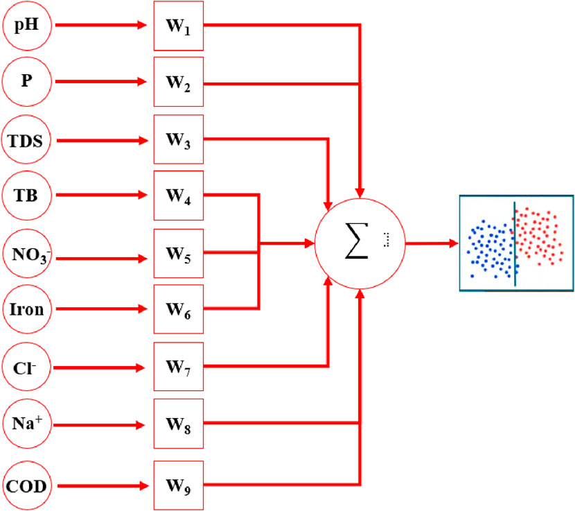
Figure 2. Structure of Perceptron units.

The outlined process involves several key steps. First, the weights and threshold are initialized to commence the training process. Next, the input features and corresponding labels are prepared to create a suitable dataset. Subsequently, training iterations are initiated, wherein each iteration includes the adjustment of weights and updating the threshold based on the Perceptron update rule. These updates are determined by comparing the predicted output with the expected label and multiplying the difference by a predefined learning rate.

The training iterations are repeated until the Perceptron achieves a satisfactory level of accuracy or converges to a solution, indicating an optimal classification model for water quality levels based on the given indicators. Once the Perceptron has been trained, predictions on new water samples can be made by applying the learned weights and threshold to the input features. The water quality level would be determined by the Perceptron’s output, which is based on the activation function (e.g., positive or negative classification).

2.3.4 ANN

ANN is a computational model inspired by the structure and functioning of biological neural networks in the human brain (Lin et al., 2022a; Zhu et al., 2023). ANN consists of interconnected artificial neurons, also known as nodes or units, organized in layers. The structure of an ANN typically comprises three main types of layers, namely, the input layer, hidden layer(s), and output layer, as shown in Figure 3. The nine water quality indicators were used as input features in the input layer. Hidden layers are intermediate layers between the input and output layers. They perform complex computations and transform the input data through a series of weighted connections. The hidden layers help the network learn and extract relevant features and patterns from the input data. As for the output layer, the number of neurons in the output layer was set as five water quality levels. It is worth noting that each neuron in the output layer represents the probability of belonging to a different class.

Figure 3

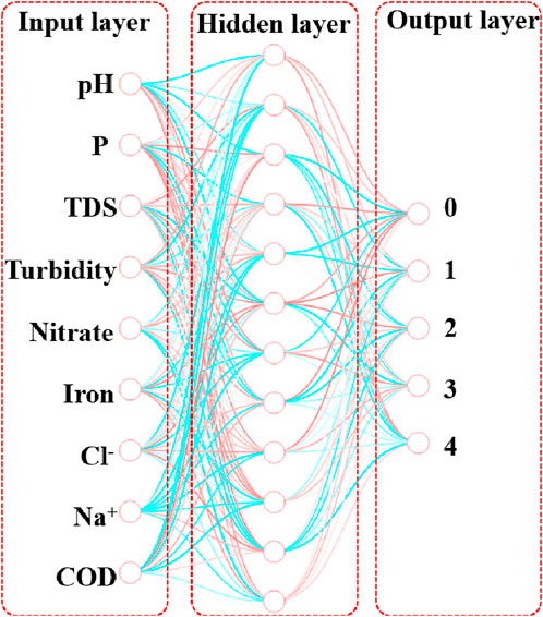
Figure 3. Structure of ANN.

2.4 Evaluation of the model performance

Accuracy, precision, recall, and F1 score were used to evaluate the performance of various models (Lin et al., 2023). They can be calculated as the following Eqs 2-7–2-10:

$\text{Accuracy}=\frac{\text{TP}+\text{TN}}{\text{TP}+\text{FN}+\text{TN}+\text{FP}},(\mathrm{2–7})$

$\text{Precision}=\frac{\text{TP}}{\text{TP}+\text{FP}},(\mathrm{2–8})$

$\text{Recall}=\frac{\text{TP}}{\text{TP}+\text{FN}},(\mathrm{2–9})$

$\text{Accuracy}=\frac{2\times \text{TP}}{2\times \text{TP}+\text{FN}+\text{FP}}.(\mathrm{2–10})$

Here, TP, TN, FN, and FP are the numbers of true positives, true negatives, false negatives, and false positives, respectively.

2.5 Bayesian optimization

Bayesian optimization is a sequential model-based optimization technique that is particularly useful for optimizing black-box functions that are expensive to evaluate (Khatamsaz et al., 2023). It combines the principles of Bayesian inference and optimization to efficiently search for the optimal solution within a given search space (Eq 2-11).

${\mathrm{x}}^{*}=\underset{\mathrm{x}\in \mathrm{X}}{\mathrm{argmin}}\mathrm{f}\left(\mathrm{x}\right),(\mathrm{2–11})$

where f(x) is the objective function to be optimized, x is a vector of input variables in the search space, and X is the search space, which represents the feasible region for the input variables. As for Eq. 2-12:

$\mathrm{D}=\left\{\left({\mathrm{x}}_{\mathrm{i}},{\mathrm{y}}_{\mathrm{i}}\right)\right\},(\mathrm{2–12})$

where x_i is a vector of input variables and y_i = f(xi) is the corresponding observed objective value. As for Eq. 2-13,

$\mathrm{P}\left(\mathrm{y}|\mathrm{x},\mathrm{D}\right)=\text{Fitmodel}\left(\mathrm{M},\mathrm{D}\right).(\mathrm{2–13})$

P is defined a probabilistic surrogate model that captures the uncertainty of the objective function, while it is assumed that the model M follows a Gaussian distribution.

A Gaussian process is an extension of multivariate Gaussian distribution to infinite dimensions. Although Gaussian distribution represents the distribution of random variables, the Gaussian process represents the distribution of functions. It can be characterized by a mean function and a covariance function, as the following Eq. 2-14:

$\mathrm{f}\left(\mathrm{x}\right)\sim \text{GP}\left(\mathrm{m}\left(\mathrm{x}\right),\mathrm{k}\left(\mathrm{x},{\mathrm{x}}^{\prime }\right)\right),(\mathrm{2–14})$

where m(x) is the mean function and k(x, x') is the kernel function.

After the tth experiment, the joint distribution between any point on the Gaussian process and the previously observed data follows a Gaussian distribution. Consequently, the predictive distribution can be derived as follows Eq. 2-15:

$\mathrm{P}\left({\mathrm{f}}_{\mathrm{t}+1}|{\mathrm{D}}_{1:\mathrm{t}},{\mathrm{x}}_{\mathrm{t}+1}\right)=\mathrm{N}\left({\mathrm{u}}_{\mathrm{t}}\left({\mathrm{x}}_{\mathrm{t}+1}\right),{{\mathrm{\sigma }}_{\mathrm{t}}}^2\left({\mathrm{x}}_{\mathrm{t}+1}\right)\right).(\mathrm{2–15})$

Typically, acquisition functions are defined such that high acquisition corresponds to potentially high values of the objective function because the prediction is high, the uncertainty is great, or both. Therefore, it can be expressed as the following Eq. 2-16:

$\text{PI}\left(\mathrm{x}\right)=\mathrm{P}\left(\mathrm{f}\left(x\right)\ge \mathrm{f}\left(x^{+}\right)+\mathrm{\xi }\right)=\mathrm{\Phi }\left(\frac{\mu \left(x\right)-f\left(x^{+}\right)-\xi }{\sigma \left(x\right)}\right).(\mathrm{2–16})$

In addition, improvement (I) is used to evaluate maximizing the expected improvement, as follows Eq. 2-17:

$\text{EI}\left(\mathrm{x}\right)=\left[\left(\mathrm{\mu }\left(\mathrm{x}\right)-\mathrm{f}\left({\mathrm{x}}^{+}\right)-\mathrm{\xi }\right)\mathrm{\Phi }\left(\mathrm{Z}\right)+\mathrm{\sigma }\left(\mathrm{x}\right)\mathrm{\varphi }\left(\mathrm{Z}\right)\right]\text{\hspace{0.17em}if\hspace{0.17em}}\mathrm{\sigma }\left(\mathrm{x}\right)>0\text{\hspace{0.17em}else\hspace{0.17em}}0.(\mathrm{2–17})$

Bayesian optimization is efficient in handling expensive and noisy objective functions by iteratively updating the surrogate model, actively exploring promising regions of the search space, and exploiting areas with potential high performance. This approach helps in finding optimal solutions with a minimal number of function evaluations.

3 Results

3.1 Impact of various water quality indicators on the WQI level

Figure 4 shows the heatmap about various water quality indicators with the water quality level by the method of Pearson correlation coefficient. It can be found that phosphate has a positive relationship with the level of water quality, with an R² value of 18%. In the context of water, “phosphate” refers to the phosphate ion (PO₄^3-), which is an important chemical species present in water. Phosphate is a compound that contains phosphorus and oxygen. It is commonly found in various forms, including orthophosphate (H₂PO₄⁻ and HPO₄^2-), which is the most prevalent form in natural water bodies (Venkata et al., 2020). Phosphate levels in water are monitored as part of water quality assessments because excessive phosphate concentrations can lead to environmental issues such as eutrophication. Eutrophication occurs when an excess of nutrients, including phosphates, stimulates the excessive growth of algae and aquatic plants, leading to oxygen depletion and negative impacts on aquatic life (Suresh et al., 2023).

Figure 4

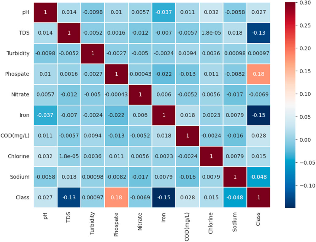
Figure 4. Heatmap about various water quality indicators with the water quality level.

Iron and TDS have a negative relationship with the water quality level, with R² of −15% and −13%, respectively. Iron exists primarily in two forms: dissolved iron (Fe²⁺ and Fe³⁺) and suspended iron. It is important to note that the concentration and distribution of iron in water can be influenced by various factors, including geological characteristics, soil types, water flow dynamics, and other environmental factors. Therefore, the predominant forms of iron may vary in different water bodies (Gao et al., 2023).

3.2 Model optimization by the method of Bayesian optimization

Figure 5 and Table 2 show the optimized hyper-parameters for SGD, AdaBoosting, Perceptron, and ANN by the method of Bayesian optimization. Figure 5A shows the value of the optimized parameters in terms of learning rate, regularization, penalty, alpha, and loss for the algorithm of SGD. As for the learning rate, it determines the step size or the rate at which the SGD parameters are updated during the optimization process (Zhang and Zhou, 2023). The result indicated that the optimized learning rate is 0.0862. Regularization is a technique used to prevent overfitting. The regularization parameter is set to 0.0161 in this study. The penalty parameter determines the type of regularization penalty to apply. The options for this were “huber,” “epsilon insensitive,” and “squared hinge.” “Huber” is a smooth penalty that combines the characteristics of both L1 and L2 penalties. However, the alpha parameter controls the weight of the regularization term in the loss function. It determines the trade-off between fitting the training data well and keeping the model parameters small. The optimized parameter of alpha is set to “l1.” In addition, the loss function measures the discrepancy between the predicted values and the actual values. It quantifies how well the model is performing during training. The value, 0.0112, represents the loss achieved by the model.

Figure 5

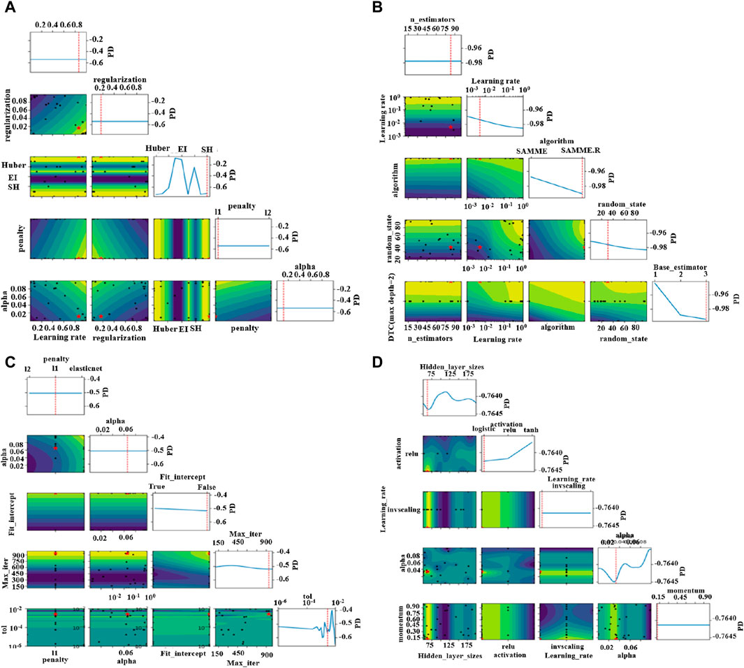
Figure 5. (A) SGD; (B) AdaBoosting; (C) Perceptron; (D) ANN. Note: DTC and PD stands for DecisionTreeClassifier and partial dependence, respectively.

Table 2

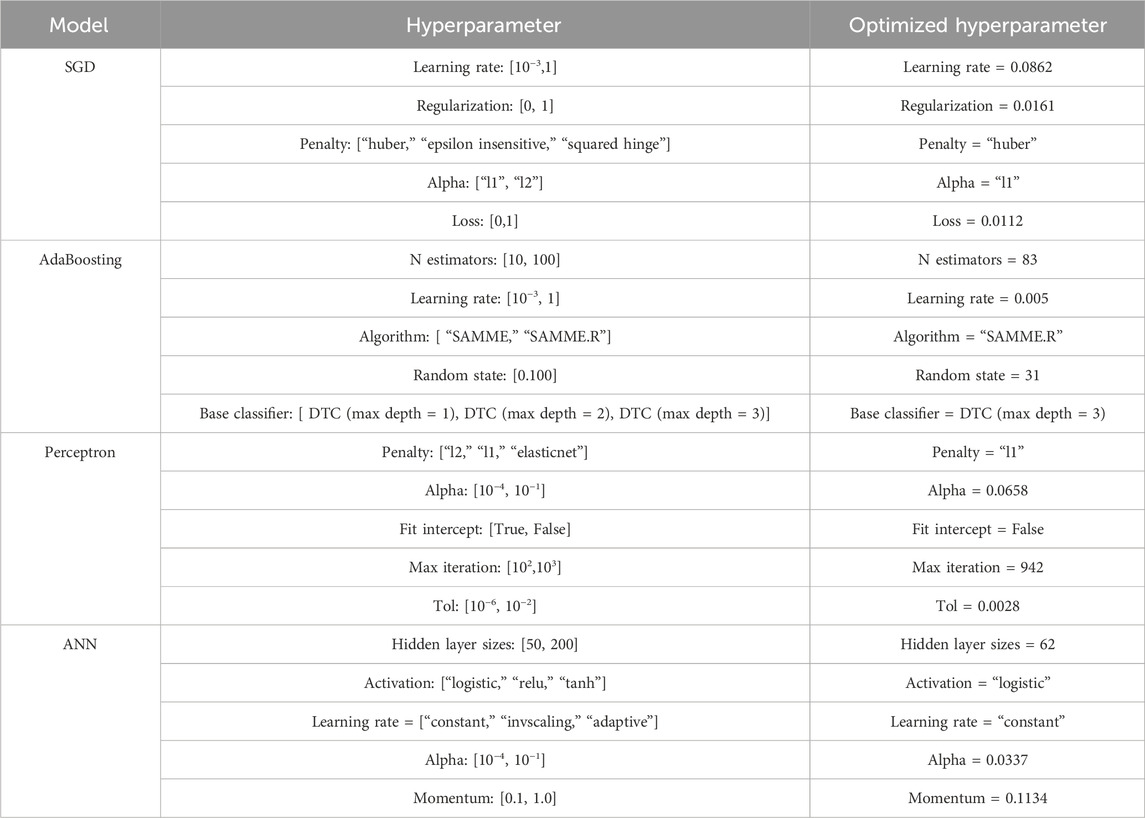
Table 2. Optimized hyperparameters for four algorithms by the method of Bayesian optimization.

Figure 5B shows the process of various hyper-parameters for the AdaBoosting algorithm. N estimators represent the number of weak classifiers or base estimators used in the AdaBoost algorithm. Weak classifiers are iteratively trained to build a strong classifier. In this case, the initial range for N estimators is 10–100, and the optimized result is 83. The learning rate controls the weight scaling of each weak classifier in the AdaBoost algorithm. It influences the contribution of each weak classifier. A smaller learning rate improves the robustness of the model but may require more weak classifiers to achieve higher performance. In this case, the initial range for the learning rate is [10⁻³, 1], and the optimized result is 0.005. The algorithm specifies the multi-class classification algorithm used in the AdaBoost algorithm. The options provided are “SAMME” and “SAMME.R.” “SAMME” is the original discrete AdaBoost algorithm with weight updates, while “SAMME.R” is a variant that incorporates class probability estimates. In this case, the optimized result is “SAMME.R.” As for the random state, this parameter determines the random seed used by the random number generator in the algorithm, controlling the randomness and reproducibility of the results. In this case, the initial range for the random state is 0–100, and the optimized result is 31. In addition, the base classifier specifies the base classifier used in the AdaBoost algorithm. The options provided are decision tree classifiers with different maximum depths: “DTC (max depth = one),” “DTC (max depth = two),” and ‘DTC (max depth = three)’. In this case, the optimized result is a decision tree classifier with a maximum depth of three.

Figure 5C shows the results of various optimized hyper-parameters for the Perceptron algorithm. Penalty determines the type of regularization penalty applied to the Perceptron algorithm. The options provided are “l2,” “l1,” and “elasticnet.” “L2” refers to ridge regularization, “l1” refers to lasso regularization, and “elasticnet” combines both the penalties. In this case, the optimized result is the “l1” penalty. The alpha parameter controls the regularization strength in the Perceptron algorithm. It represents the constant that multiplies the regularization term. The initial range for alpha is [10⁻⁴, 10⁻¹], and the optimized result is 0.0658. Fit intercept determines whether to calculate the intercept for the Perceptron algorithm. If set to true, an additional feature with a constant value 1 is added to the input data. If set to false, no intercept is calculated. In this case, the optimized result is Fit intercept = False. The max iteration parameter defines the maximum number of iterations for the Perceptron algorithm to converge. It represents the maximum number of passes over the training data. The initial range for max iteration is [10², 10³], and the optimized result is 942. The “tol” parameter specifies the tolerance for convergence in the Perceptron algorithm. It determines the criterion for early stopping when the change in the model’s coefficients is below the tolerance value. The initial range for tolerance is [10⁻⁶, 10⁻²], and the optimized result is 0.0028.

The results for the optimized parameters in the ANN model by the method of Bayesian optimization are shown in Figure 5D. The hidden layer sizes define the number of neurons in each hidden layer of the artificial neural network. The range provided is [50, 200]. The result indicated that the optimal number of neurons in the hidden layer is 62. The activation parameter specifies the activation function used in the artificial neural network. The options provided are “logistic,” “relu,” and “tanh.” “Logistic” refers to the logistic sigmoid function, “relu” refers to the rectified linear unit function, and “tanh” refers to the hyperbolic tangent function. In this case, the logistic sigmoid function is chosen as the activation function. The learning rate determines the learning rate schedule for updating the weights of the neural network during training. The options provided are “constant,” “invscaling,” and “adaptive.” “Constant” keeps the learning rate constant throughout the training process, “invscaling” decreases the learning rate gradually over time, and “adaptive” adjusts the learning rate automatically based on the validation score. In this case, the optimized learning rate is constant. The alpha parameter represents the L2 regularization term’s strength in the neural network’s cost function. It controls the amount of weight decay applied to prevent overfitting. The initial range for alpha is [10⁻⁴, 10⁻¹], and the optimized result is Alpha = 0.0337. The momentum parameter is used to accelerate the optimization process by adding a fraction of the previous weight update to the current update. It helps the model overcome local minima and converge faster. The initial range for momentum is [0.1, 1.0], and the value of the optimized momentum result is 0.1134.

3.3 Comparison of various models for the performance of the classification of the water quality level

3.3.1 Confusion matrix

Figure 6A ∼ Figure 6D show the confusion matrix on the test dataset from the algorithm of SGD, AdaBoosting, Perceptron, and ANN, respectively. A confusion matrix is a table that summarizes the performance of a classification model on a test dataset (Lin et al., 2022b). It shows the predicted labels versus the actual labels and provides valuable insights into the model’s accuracy and errors. Taking SGD algorithms as the example in Figure 6A, the confusion matrix for SGD consists of diagonal values, lower-left values, and upper-right values. As for the diagonal values, the values on the diagonal represent the number of correctly classified instances for each class. For example, 749 points were correctly classified to class 3. In other words, these values indicate the true positives (TP), where the predicted class matches the actual class.

Figure 6

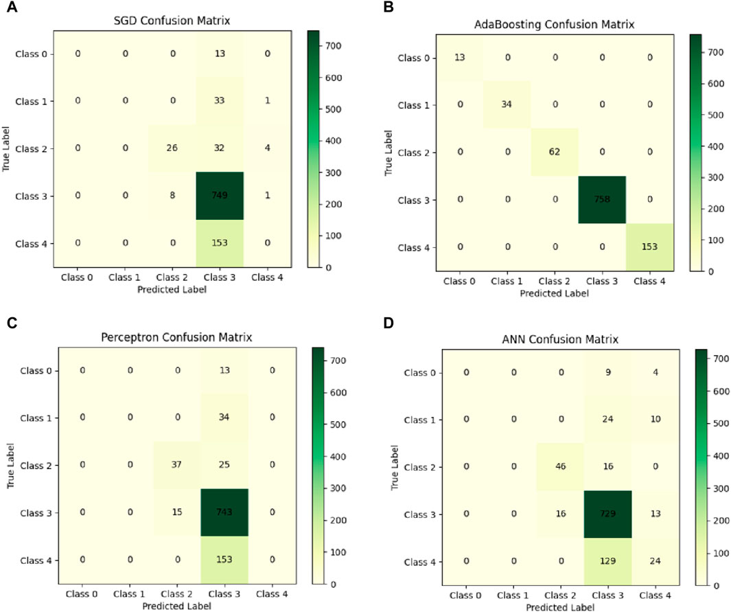
Figure 6. Confusion matrix on the test dataset: (A) SGD; (B) AdaBoosting; (C) Perceptron; (D) ANN.

The values in the lower-left portion of the matrix represent the number of instances that were incorrectly classified as negative (false negatives, FN). To be accurate, eight points and 153 points were incorrectly classified as class 3 and class 4, respectively. These are cases where the model predicted the instance as negative, but it actually belonged to a positive class (class 2 and class 3, respectively). Finally, the values in the upper-right portion of the matrix represent the number of instances that were incorrectly classified as positive (false positives, FP). For example, 13 points were wrongly recognized as class 0, which actually belonged to class 3.

Compared with Figure 6A, Figure 6C, and Figure 6D, the diagonal values in Figure 6B were higher than that in the others’ confusion matric, which indicated that AdaBoosting may have best the performance compared to other algorithms for the classification of the water quality level. To quantitatively evaluate the performance of various algorithms, indexes like accuracy, precision, recall, and F1 score were employed.

3.3.2 Accuracy, precision, recall, and F1 score

Figure 7 presents the performance evaluation of various algorithms on the test dataset, focusing on the accuracy, precision, recall, and F1 scores. Accuracy quantifies the overall correctness of model predictions by assessing the ratio of correctly classified instances to the total number of instances (Lin et al., 2022c). The results in Figure 7A demonstrate that AdaBoosting achieves the highest accuracy (100%) among the models, followed by ANN (78.33%), Perceptron (76.47%), and SGD (76.37%). The perfect accuracy achieved by AdaBoosting showcases its exceptional performance on the given dataset.

Figure 7

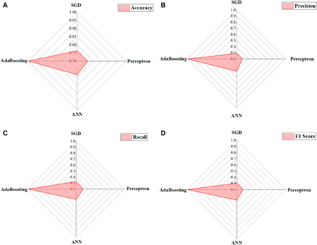
Figure 7. Performance of various algorithms on the test dataset in terms of (A) accuracy; (B) precision; (C) recall; (D) F1 scores.

Precision evaluates a model’s ability to accurately identify positive instances among those predicted as positive (Lin et al., 2022c). It emphasizes the quality of positive predictions. As shown in Figure 7B, AdaBoosting exhibits the highest precision, followed by ANN, Perceptron, and SGD. Specifically, SGD achieves a precision of 28.98%, indicating that only 28.98% of instances predicted as positive by the SGD model are truly positive. Perceptron displays a slightly higher precision of 29.58%, outperforming SGD, with 29.58% of instances predicted as positive being true positives. ANN demonstrates further improvement, achieving a precision of 40.33%, surpassing both SGD and Perceptron. Remarkably, AdaBoosting achieves a perfect precision score of 100%, accurately classifying all positive instances with no false positives.

Recall, also known as sensitivity or true positive rate, measures a model’s ability to correctly identify positive instances out of the actual positive instances. It focuses on capturing all positive instances (Lin et al., 2022c). As shown in Figure 7C, Perceptron achieves a recall of 31.54%, indicating its ability to correctly identify 31.54% of the actual positive instances in the test dataset. SGD shows a slightly higher recall of 32.70%, performing slightly better by correctly identifying approximately 32.70% of the actual positive instances. On the other hand, ANN exhibits significant improvement with a recall of 37.21%, outperforming both SGD and Perceptron by correctly identifying approximately 37.21% of the actual positive instances. AdaBoosting achieves a perfect recall value of 1, indicating its ability to correctly identify all positive instances, resulting in 100% recall. Overall, AdaBoosting achieves the highest recall among the models, followed by ANN, Perceptron, and SGD. The perfect recall achieved by AdaBoosting emphasizes its capability to identify all positive instances in the test dataset. SGD and Perceptron exhibit lower recall values, suggesting the potential for missing a significant number of actual positive instances. Conversely, ANN demonstrates improved recall, reflecting its enhanced overall performance in capturing positive instances.

The F1 score serves as a comprehensive metric by harmonizing precision and recall, making it particularly valuable in cases of data imbalance or when both precision and recall carry equal importance (Lin et al., 2022c). As shown in Figure 7D, SGD achieves an F1 score of 30.62%, denoting a balanced performance in correctly classifying positive instances. This score represents the harmonic mean of precision and recall and reflects the SGD model’s overall capability in accurately identifying positive instances. Similarly, the Perceptron model demonstrates an F1 score of 30.20%, signifying comparable performance to SGD, with a similar harmonic mean of precision and recall. Conversely, the ANN model exhibits notable improvement with an F1 score of 37.06%, surpassing both SGD and Perceptron. This higher F1 score signifies the ANN model’s superior balance between precision and recall. Consequently, the ANN model displays enhanced overall performance and effectiveness in classification. Impressively, AdaBoosting achieves a perfect F1 score of 1, signifying its exceptional ability to accurately classify positive instances. This score indicates the optimal balance achieved between precision and recall by the AdaBoosting model, resulting in unparalleled classification performance. Overall, AdaBoosting attains the highest F1 score among the evaluated models, followed by ANN, Perceptron, and SGD. The perfect F1 score achieved by AdaBoosting underscores its remarkable precision and recall balance, further emphasizing its accurate classification of positive instances. Although SGD and Perceptron exhibit lower F1 scores, they present opportunities for improvement in achieving a better balance between precision and recall. Conversely, the ANN model showcases an improved F1 score, highlighting its superior overall performance and effectiveness in classification.

In conclusion, compared with the other algorithms, AdaBoosting achieves the best performance for water quality level classification, as evidenced by its superior accuracy (100%), precision (100%), recall (100%), and F1 score (100%).

3.4 Identification of key water quality indicators

Figure 8 presents the feature importance analysis conducted using the AdaBoosting model on various water quality indicators. The results reveal the top four important factors for water quality level classification: COD (0.684), phosphate (0.119), iron (0.112), and TDS (0.084), as depicted in Figure 8A.

Figure 8

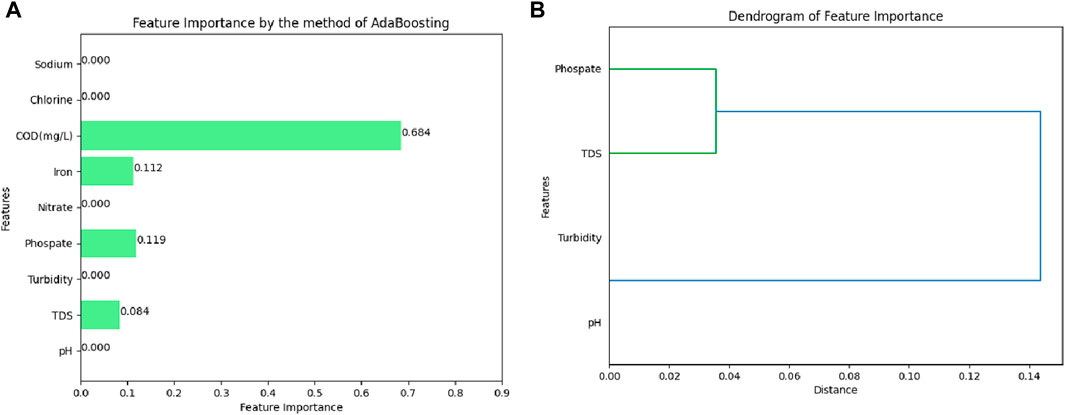
Figure 8. Identification of key water quality indicators in terms of features importance from the model of AdaBoosting: (A) bar chart; (B) dendrogram.

COD is a crucial parameter in assessing the water quality, representing the amount of oxygen required to chemically oxidize the organic and inorganic compounds in water. Higher COD values indicate elevated concentrations of organic and inorganic pollutants, suggesting poorer water quality. The significant importance of COD in the AdaBoosting model highlights its pivotal role in classifying water quality levels. This finding aligns with the existing literature, which emphasizes COD as a primary indicator of water pollution (Ehteram et al., 2024).

Phosphate is a common nutrient found in water bodies that can lead to eutrophication and water quality degradation when present at excessive levels due to pollution sources such as agricultural runoff or wastewater discharge. The inclusion of phosphate as an important feature in the AdaBoosting model signifies its significance in determining water quality levels. Phosphate levels are monitored closely in many water bodies’ quality studies due to their impact on aquatic ecosystems (Uddin et al., 2024a).

Iron is a naturally occurring element in water from geological sources or human activities. It can impact the water quality and taste and cause discoloration. Its relevance as an important feature in the AdaBoosting model underlines its influence on water quality classification. The presence of iron in water, particularly in high concentrations, is often associated with industrial pollution and natural leaching processes (Uddin et al., 2023a).

TDS refers to the concentration of inorganic salts, minerals, and other dissolved substances in water. High TDS levels may indicate water pollution, excessive mineral content, or contamination. The incorporation of TDS as an important feature in the AdaBoosting model underscores its influence on water quality level classification. TDS is a widely used parameter in water quality assessments to evaluate the salinity and overall chemical content of water (Uddin et al., 2023b).

Collectively, these four features—COD, phosphate, iron, and TDS—provide valuable information for the AdaBoosting model in accurately classifying water quality levels. Their respective importance signifies their contribution to the model’s predictive power in determining the quality of water samples.

Dendrograms, hierarchical tree-like structures, serve as valuable tools for illustrating the relationships and similarities between features or samples. In Figure 8B, the dendrogram depicts the feature importance, specifically showcasing the grouping of phosphate and TDS in one branch and pH and turbidity in another branch. The distance between these branches signifies the dissimilarity or separation between these groups of features. The grouping of phosphate and TDS within the same branch implies a higher level of correlation between these two features, suggesting that variations or changes in phosphate levels are likely to coincide with similar variations in TDS levels. Consequently, there exists a potential relationship or co-occurrence between these two parameters regarding their impact on water quality. Similarly, the grouping of pH and turbidity in the same branch suggests a correlation or similarity between these two features, indicating their combined influence on water quality.

By identifying and discussing these key water quality indicators, our study provides a comprehensive understanding of the factors that are most influential in determining water quality levels, offering valuable insights for water resource management and policy-making.

4 Discussion

4.1 Novelty and contributions

This study offers several novel contributions compared to the existing literature. First, it uniquely integrates Bayesian optimization to dynamically tune hyperparameters in different machine learning algorithms, addressing the challenge of parameter optimization more effectively than the traditional methods. Additionally, unlike previous studies, this research considers a broader range of water quality parameters, providing a more holistic evaluation of water quality. By employing AdaBoosting with optimized hyperparameters, the study achieves outstanding performance metrics (100% accuracy, precision, recall, and F1 score) that surpass the existing models in the literature.

Moreover, this is the first study to apply these advanced machine learning techniques specifically to Korattur Lake, offering valuable insights for local water quality management and conservation efforts. Compared to previous studies that utilized models like ANFIS, RBF-ANN, and MLP-ANN, our approach with AdaBoosting shows superior performance in terms of accuracy and other evaluation metrics (Uddin et al., 2024a; Sajib et al., 2024). The use of Bayesian optimization further enhances the model’s efficiency and effectiveness, addressing limitations found in grid search and random search methods.

4.2 Advantages and limitations in terms of methodology

Bayesian optimization offers higher efficiency and better performance compared to traditional grid search and random search methods, significantly enhancing the hyperparameter tuning process (Uddin et al., 2023a; Uddin et al., 2023b). The AdaBoosting model achieves perfect scores in accuracy, precision, recall, and F1, demonstrating its robustness and reliability. Additionally, the comprehensive feature importance analysis identifies key water quality indicators, providing actionable insights for water resource management.

Despite these advantages, there are limitations to consider. Although the models achieve a high performance, their interpretability can be challenging. Efforts to enhance model interpretability, such as using SHAP (SHapley Additive exPlanation) values, could be beneficial in future studies. Furthermore, although the model performs exceptionally well for Korattur Lake, its generalizability to other water bodies needs further investigation. Future work should focus on validating the model in different geographical locations with varying water quality parameters.

4.3 Perspective of the future application

Future applications of this study include the integration of the optimized AdaBoosting algorithm into real-time water quality monitoring systems to provide accurate and timely classifications of water quality. This can enable quick responses to changes or deterioration in water conditions. Additionally, by identifying key factors such as COD, phosphate, iron, and TDS, the model can be used in predictive maintenance to anticipate and mitigate issues, thereby enhancing water resource management. The findings can also inform policymakers and regulatory bodies to develop targeted regulations and policies for water quality management based on the important factors identified. Furthermore, the methodology and results can serve as a reference for further research in environmental science and engineering and as a teaching resource for related courses. Lastly, this approach can be adapted and applied to classify the water quality in other lakes or water bodies, aiding in the broader assessment and management of water resources in various geographical locations.

5 Conclusion

This study used different machine learning models integrated with Bayesian optimization to classify the water quality in Korattur Lake. The results show that that the optimized hyperparameters of N_estimators, learning rate, algorithms, random state, and base classifier for the AdaBoosting algorithm by the method of Bayesian optimization are 83, 0.005, SAMME. R, 31, and DTC with a maximum depth of 3, respectively. Compared with the other algorithms, AdaBoosting achieves the best performance for water quality level classification, as evidenced by its superior accuracy (100%), precision (100%), recall (100%), and F1 score (100%). The top four important factors for water quality level classification are COD (0.684), phosphate (0.119), iron (0.112), and TDS (0.084). In addition, variations or changes in phosphate levels are likely to coincide with similar variations in TDS levels. Future applications of this study include the integration of the optimized AdaBoosting algorithm into real-time water quality monitoring systems to provide accurate and timely classifications of water quality. The findings can also inform policymakers and regulatory bodies to develop targeted regulations and policies for water quality management based on the important factors identified. Furthermore, the methodology and results can serve as a reference for further research in environmental science and engineering and as a teaching resource for related courses. Lastly, this approach can be adapted and applied to classify the water quality in other lakes or water bodies, aiding in the broader assessment and management of water resources in various geographical locations.

Data availability statement

The raw data supporting the conclusion of this article will be made available by the author, without undue reservation.

Author contributions

LZ: writing–original draft and writing–review and editing.

Funding

The author declares that no financial support was received for the research, authorship, and/or publication of this article.

Conflict of interest

Author LZ was employed by Guangzhou Wosu Environmental Technology Co., Ltd.

Publisher’s note

All claims expressed in this article are solely those of the authors and do not necessarily represent those of their affiliated organizations, or those of the publisher, the editors, and the reviewers. Any product that may be evaluated in this article, or claim that may be made by its manufacturer, is not guaranteed or endorsed by the publisher.

References

Ahmed, U., Mumtaz, R., Anwar, H., Shah, A. A., Irfan, R., and García-Nieto, J. (2019). Efficient water quality prediction using supervised machine learning. Water 11, 2210. doi:10.3390/w11112210

CrossRef Full Text | Google Scholar

Andrychowicz, M., Misha, D., Sergio, G. C., Mattew, W. H., David, P., Tom, S., et al. (2016). “Learning to learn by gradient descent by gradient descent,” in 30th conference on neural information processing system (Spain: Barcelona).

Google Scholar

Belghit, A., Lazri, M., Ouallouche, F., Labadi, K., and Ameur, S. (2023). Optimization of One versus All-SVM using AdaBoost algorithm for rainfall classification and estimation from multispectral MSG data. Adv. Space Res. 71, 946–963. doi:10.1016/j.asr.2022.08.075

CrossRef Full Text | Google Scholar

Bhateria, R., and Jain, D. (2016). Water quality assessment of lake water: a review. Sustain. Water Resour. Manag. 2, 161–173. doi:10.1007/s40899-015-0014-7

CrossRef Full Text | Google Scholar

Bui, D. T., Khosravi, K., Tiefenbacher, J., Nguyen, H., and Kazakis, N. (2020). Improving prediction of water quality indices using novel hybrid machine-learning algorithms. Sci. Total Environ. 721, 137612. doi:10.1016/j.scitotenv.2020.137612

PubMed Abstract | CrossRef Full Text | Google Scholar

Chen, L., Wu, T., Wang, Z., Lin, X., and Cai, Y. (2023). A novel hybrid BPNN model based on adaptive evolutionary Artificial Bee Colony Algorithm for water quality index prediction. Ecol. Indic. 146, 109882. doi:10.1016/j.ecolind.2023.109882

CrossRef Full Text | Google Scholar

Ehteram, M., Ahmed, A. N., Sherif, M., and El-Shafie, A. (2024). An advanced deep learning model for predicting water quality index. Ecol. Indic. 160, 111806. doi:10.1016/j.ecolind.2024.111806

CrossRef Full Text | Google Scholar

Gao, Y., Zhuang, Y., Wu, S., Qi, Z., Li, P., and Shi, B. (2023). Enhanced disinfection byproducts formation by fine iron particles intercepted in household point-of-use facilities. Water Res. 243, 120320. doi:10.1016/j.watres.2023.120320

PubMed Abstract | CrossRef Full Text | Google Scholar

González, L. D., and Zavala, V. M. (2023). New paradigms for exploiting parallel experiments in Bayesian optimization. Comput. Chem. Eng. 170, 108110. doi:10.1016/j.compchemeng.2022.108110

CrossRef Full Text | Google Scholar

Granata, F., Di Nunno, F., and Pham, Q. B. (2024). A novel additive regression model for streamflow forecasting in German rivers. Results Eng. 22, 102104. doi:10.1016/j.rineng.2024.102104

CrossRef Full Text | Google Scholar

Khatamsaz, D., Vela, B., Singh, P., Johnson, D. D., Allaire, D., and Arróyave, R. (2023). Bayesian optimization with active learning of design constraints using an entropy-based approach. npj Comput. Mater. 9 (1), 49. doi:10.1038/s41524-023-01006-7

CrossRef Full Text | Google Scholar

Lin, K., Zhao, Y., and Kuo, J. H. (2023). Data-driven models applying in household hazardous waste: amount prediction and classification in Shanghai. Ecotoxicol. Environ. Saf. 263, 115249. doi:10.1016/j.ecoenv.2023.115249

PubMed Abstract | CrossRef Full Text | Google Scholar

Lin, K., Zhao, Y., Kuo, J.-H., Deng, H., Cui, F., Zhang, Z., et al. (2022a). Toward smarter management and recovery of municipal solid waste: a critical review on deep learning approaches. J. Clean. Prod. 346, 130943. doi:10.1016/j.jclepro.2022.130943

CrossRef Full Text | Google Scholar

Lin, K., Zhao, Y., Tian, L., Zhao, C., Zhang, M., and Zhou, T. (2021). Estimation of municipal solid waste amount based on one-dimension convolutional neural network and long short-term memory with attention mechanism model: a case study of Shanghai. Sci. Total Environ. 791, 148088. doi:10.1016/j.scitotenv.2021.148088

PubMed Abstract | CrossRef Full Text | Google Scholar

Lin, K., Zhao, Y., Zhang, M., Shi, W., and Kuo, J. H. (2022b). Data-driven models employed to waste plastic in China: generation, classification, and environmental assessment. J. Industrial Ecol. 27, 170–181. doi:10.1111/jiec.13340

CrossRef Full Text | Google Scholar

Lin, K., Zhou, T., Gao, X., Li, Z., Duan, H., Wu, H., et al. (2022c). Deep convolutional neural networks for construction and demolition waste classification: VGGNet structures, cyclical learning rate, and knowledge transfer. J. Environ. Manag. 318, 115501. doi:10.1016/j.jenvman.2022.115501

CrossRef Full Text | Google Scholar

Najah Ahmed, A., Binti Othman, F., Abdulmohsin Afan, H., Khaleel Ibrahim, R., Ming Fai, C., Shabbir Hossain, M., et al. (2019). Machine learning methods for better water quality prediction. J. Hydrology 578, 124084. doi:10.1016/j.jhydrol.2019.124084

CrossRef Full Text | Google Scholar

Ratsch, G., Onoda, T., and Muller, K.-R. (2001). Soft margins for AdaBoost. Mach. Learn. 42, 287–320. doi:10.1023/a:1007618119488

CrossRef Full Text | Google Scholar

Sajib, A. M., Diganta, M. T. M., Moniruzzaman, M., Rahman, A., Dabrowski, T., Uddin, M. G., et al. (2024). Assessing water quality of an ecologically critical urban canal incorporating machine learning approaches. Ecol. Inf. 80, 102514. doi:10.1016/j.ecoinf.2024.102514

CrossRef Full Text | Google Scholar

Shams, M. Y., Elshewey, A. M., El-kenawy, E.-S. M., Ibrahim, A., Talaat, F. M., and Tarek, Z. (2023). Water quality prediction using machine learning models based on grid search method. Multimedia Tools Appl. 83, 35307–35334. doi:10.1007/s11042-023-16737-4

CrossRef Full Text | Google Scholar

Suresh, K., Tang, T., van Vliet, M. T. H., Bierkens, M. F. P., Strokal, M., Sorger-Domenigg, F., et al. (2023). Recent advancement in water quality indicators for eutrophication in global freshwater lakes. Environ. Res. Lett. 18, 063004. doi:10.1088/1748-9326/acd071

CrossRef Full Text | Google Scholar

Uddin, M. G., Nash, S., Rahman, A., Dabrowski, T., and Olbert, A. I. (2024a). Data-driven modelling for assessing trophic status in marine ecosystems using machine learning approaches. Environ. Res. 242, 117755. doi:10.1016/j.envres.2023.117755

PubMed Abstract | CrossRef Full Text | Google Scholar

Uddin, M. G., Nash, S., Rahman, A., and Olbert, A. I. (2023a). Assessing optimization techniques for improving water quality model. J. Clean. Prod. 385, 135671. doi:10.1016/j.jclepro.2022.135671

CrossRef Full Text | Google Scholar

Uddin, M. G., Nash, S., Rahman, A., and Olbert, A. I. (2023b). A novel approach for estimating and predicting uncertainty in water quality index model using machine learning approaches. Water Res. 229, 119422. doi:10.1016/j.watres.2022.119422

PubMed Abstract | CrossRef Full Text | Google Scholar

Uddin, M. G., Rahman, A., Rosa Taghikhah, F., and Olbert, A. I. (2024b). Data-driven evolution of water quality models: an in-depth investigation of innovative outlier detection approaches-A case study of Irish Water Quality Index (IEWQI) model. Water Reseach 255, 121499. doi:10.1016/j.watres.2024.121499

CrossRef Full Text | Google Scholar

Venkata, V. P. D., Y Venkataramana, L., Kumar, P. S., Prasannamedha, G., Soumya, K., and A.j., P. (2020). Water quality analysis in a lake using deep learning methodology: prediction and validation. Int. J. Environ. Anal. Chem. 102, 5641–5656. doi:10.1080/03067319.2020.1801665

CrossRef Full Text | Google Scholar

Yan, T., Zhou, A., and Shen, S. L. (2023). Prediction of long-term water quality using machine learning enhanced by Bayesian optimisation. Environ. Pollut. 318, 120870. doi:10.1016/j.envpol.2022.120870

PubMed Abstract | CrossRef Full Text | Google Scholar

Zhang, J., Li, C., Yin, Y., Zhang, J., and Grzegorzek, M. (2023). Applications of artificial neural networks in microorganism image analysis: a comprehensive review from conventional multilayer perceptron to popular convolutional neural network and potential visual transformer. Artif. Intell. Rev. 56, 1013–1070. doi:10.1007/s10462-022-10192-7

PubMed Abstract | CrossRef Full Text | Google Scholar

Zhang, Z., and Zhou, S. (2023). Adaptive proximal SGD based on new estimating sequences for sparser ERM. Inf. Sci. 638, 118965. doi:10.1016/j.ins.2023.118965

CrossRef Full Text | Google Scholar

Zhu, S., Di Nunno, F., Ptak, M., Sojka, M., and Granata, F. (2023). A novel optimized model based on NARX networks for predicting thermal anomalies in Polish lakes during heatwaves, with special reference to the 2018 heatwave. Sci. Total Environ. 905, 167121. doi:10.1016/j.scitotenv.2023.167121

PubMed Abstract | CrossRef Full Text | Google Scholar

Zhu, S., Di Nunno, F., Sun, J., Sojka, M., Ptak, M., and Granata, F. (2024). An optimized NARX-based model for predicting thermal dynamics and heatwaves in rivers. Sci. Total Environ. 926, 171954. doi:10.1016/j.scitotenv.2024.171954

PubMed Abstract | CrossRef Full Text | Google Scholar