 Zhang Jianmin
 Yang Yang
 Kao Xiaoxuan
94% of researchers rate our articles as excellent or good
Learn more about the work of our research integrity team to safeguard the quality of each article we publish.
Find out more
ORIGINAL RESEARCH article
Front. Environ. Sci., 15 July 2024
Sec. Environmental Economics and Management
Volume 12 - 2024 | https://doi.org/10.3389/fenvs.2024.1431324
This article is part of the Research TopicUrban Carbon Emissions and Anthropogenic ActivitiesView all 19 articles
Cities are the core carriers and key positions to achieve the dual carbon goals. It is of great significance to explore whether promoting urbanization can improve carbon emission performance, which is of great significance to comprehensively promote the goal of carbon neutrality. Based on the panel data from 2006 to 2021, this paper analyzes the spatial autocorrelation of carbon emission performance per unit space and the impact mechanism of urbanization process on it. The fixed-effect model was further used to identify the influencing factors of spatial carbon emission performance. The results show that: 1) China’s carbon emission performance per unit space is declining year by year. 2) There is a strong positive spatial correlation and stable path dependence on the performance of carbon emissions per unit space in each region. 3) To a certain extent, increasing the level of urbanization will reduce the carbon emission performance per unit space. 4) The urbanization process has a spatial spillover effect on the carbon emission performance per unit space of surrounding provinces, and the spatial spillover effect of industrial structure and energy consumption structure is more obvious than that of economic level, population density and urbanization rate. Based on the conclusions, this paper puts forward specific policy suggestions to reduce the carbon emission performance per unit space to help the low-carbon development of cities.
With the acceleration of urbanization and the increasing population on a global scale, regional development is facing more and more challenges, one of which is environmental problems. Studies have shown that cities are the main source of the highest energy consumption and greenhouse gas emissions. The process of urbanization is directly related to environmental indicators such as urban land use efficiency, traffic congestion, energy consumption and carbon emissions (Ishii et al., 2009). In 2020, China put forward the goal of carbon peak and carbon neutrality, that is, China is committed to achieving carbon emission peak before 2030 and carbon neutrality before 2060 (Zhuang, 2021). As an important indicator of urban planning and management, urbanization plays an important role in the sustainable development and environmental protection of cities and regions. Therefore, building low-carbon cities has become an inevitable choice for China to embrace climate change and promote the development of a low-carbon economy.
At present, the discussion on carbon emissions mainly focuses on the influencing factors of carbon emissions (Song and Lu, 2009; Lin and Liu, 2010; Chen et al., 2014), characteristics (Hu et al., 2008), and estimation methods (Feng, 2011; Wang, 2012; Jing et al., 2019), among which carbon emission performance has become the focus of the discussion. Liu Guoping (Liu and Zhu, 2013) proposed that carbon emission welfare performance is the economic and social welfare output per unit of carbon emissions based on the ecological welfare performance theory and the steady-state economic theory of Herman Daly (Daly, 1974). Yan Wentao et al. further expanded carbon performance into energy utilization performance, air environment performance, water environment performance, biodiversity performance, and soil environmental performance. It is also applied to the study of environmental performance, root causes of environmental problems, and optimal spatial structure (Yan et al., 2012). Hua Jian et al. define carbon emission performance as two meanings based on reality and expectation. Reality: Carbon performance refers to the ratio between the actual expected output per unit of carbon emissions and the expected output of the optimal production technology. Expectation: Carbon emission performance is the ratio of the theoretical carbon emission boundary to the actual carbon emission (Hua et al., 2013).
Studies have shown that about 50% of CO2 emissions from residential transportation can be attributed to urban morphological factors such as urban form, land structure, building type, and transportation network, and urbanization has a non-negligible impact on carbon emissions (Zuo et al., 2022). Based on the quantitative relationship between urban spatial form and carbon emissions, Ewing pointed out that urban spatial structure indirectly affects residents’ emissions through intermediate factors (Ewing and Rong, 2008). Ou et al. analyzed the relationship between carbon emissions and spatial structure and morphology, and showed that single-center cities have higher LPIs and are more prone to congestion and high carbon emissions (Ou et al., 2013). Zahabi, et al. showed that improving the urbanization process and land use mix can reduce greenhouse gas emissions (Zahabi et al., 2012). Hilber et al. pointed out that increasing population density and increasing the number of automobiles can lead to a proportional decrease in CO2 emissions (Hilber and Palmer, 2014). In fact, carbon emissions are not only affected by the local urbanization process, but also by the spatial spillover effects brought by the surrounding areas. Du Huibin pointed out that China’s regional carbon emission performance shows an obvious regional cluster phenomenon, and there is a strong spatial positive correlation (Du et al., 2013).
The above studies focus on the impact and mechanism of local urbanization on carbon emissions, but lack of in-depth discussion on spatial externalities. There is still insufficient research on the positive and negative effects of regional spillover on carbon emissions. The central problem of Spatial Economics is to explain the agglomeration of economic activities in geographic space (Liang, 2005). Ecological Geography the laws and mechanisms of the relationship between various components of the ecosystem and the geospatial distribution pattern of ecological processes (Fu and Fu, 2019). In order to introduce the land scale factor, this paper proposes the carbon emission performance per unit space from the perspective of Spatial Economics and Ecological Geography, and defines it as the ratio of carbon emissions or environmental load to GDP within a certain spatial range. At the same time, the positive effects of economic and welfare output per unit of carbon emissions and the negative effects of environmental load per unit space are considered, and the relationship between land resource input and environmental impact targets is studied. It includes the control of the scale of carbon emissions in a certain space, as well as the restrictions on resource input and emission output intensity targets, which more comprehensively reflects the dimensions and complexity of carbon emission performance. Based on the theory of ecological economics and the perspective of spatial interaction, the Spatial Dubin Model is constructed by using econometric methods to study the logical relationship between urbanization process and carbon emission performance per unit space. At the same time, this paper explores the impact mechanism of spatial spillover effects between regions on the carbon emission performance per unit space, aiming to put forward spatial planning and policy suggestions for regional environmental constraint indicators, help China achieve the dual carbon goals in an orderly and efficient manner, promote the coordination of economy, society and environment, and achieve sustainable development.
The impact of urbanization on the performance of carbon emissions per unit space mainly comes from the changes and fluctuations in economy, population, energy, and industrial structure (Li and Zhou, 2012; Sun et al., 2013; Shen et al., 2023). Both the theory of ecological modernization and the theory of urban environmental transformation believe that with the evolution of urban development, the quality of urban environment will deteriorate first and then improve (Zhang et al., 2016). The growth of GDP is usually accompanied by an increase in energy consumption, including an increase in energy demand for industrial production, transportation, and residential life. The consumption of these energy sources is often accompanied by large amounts of greenhouse gas emissions, especially carbon dioxide. However, when the level of economic agglomeration and urbanization reach a certain threshold, it will show the dual effects of energy conservation and emission reduction at the same time, and can have a direct impact on carbon emissions through various positive externalities (Shao et al., 2019). With the improvement of economic level and technical level, the industrial production mode has undergone intelligent changes. Under the process of urbanization, changes in residents’ lifestyles, such as the increase in the level of electrification, have a certain negative impact on the performance of spatial carbon emissions. That is, it can reduce the level of carbon emission performance per unit space. At the same time, the development of China’s three industries also has a certain impact on carbon emissions. An increase in the number of employees and capital stock in the primary and tertiary sectors leads to a reduction in carbon emissions. The GDP, capital stock, and employees of the secondary industry have a positive effect on carbon emissions (Zheng and Liu, 2011), so reducing the proportion of the secondary industry structure can effectively reduce the carbon emission performance level of urban space.
However, Population growth will lead to an increase in greenhouse gas emissions, on the one hand, a large total population will increase the demand for energy, which in turn will lead to more and more greenhouse gas emissions from energy consumption. On the other hand, the population is growing rapidly, the supply of existing resources is likely to exceed demand, the environment such as forests are destroyed, and the use of land is changing, resulting in an increase in carbon dioxide emissions (Zhu et al., 2010). With the evolution of urbanization, changes in energy consumption structure, the spread of urban civilization and the improvement of technological level will have a restraining effect on carbon emissions. However, China’s coal-dominated energy consumption structure makes coal account for a major share of energy consumption. Even if the energy structure is changed through energy substitution, it is mainly the substitution of oil for coal. The proportion of non-fossil energy use is still low, and oil is a carbonaceous fossil fuel second only to coal, and still has a high level of carbon emissions (Sun, 2010). Therefore, with the advancement of urbanization, the growth of population density and the adjustment of energy structure will still increase the overall carbon emission level, which will have a positive impact on the carbon emission performance level per unit space.
Hypothesis. H1: Increasing the level of urbanization to a certain extent will reduce the carbon emission performance per unit space. Specifically, economic level, industrial structure, and urbanization rate have a negative impact on the carbon emission performance per unit space, while population density and energy consumption structure have a positive impact on the carbon emission performance per unit space.
Carbon emissions are not only affected by the local urbanization process, but also by the spatial spillover effect brought by the surrounding areas. Adjacent areas have similar cultural environments, social conditions, and economic levels. The frequent flow of transportation, population, technology, etc., creates an agglomeration effect between regions, resulting in interactions. In this process, carbon emissions will be diffused and transferred to the surrounding areas along with the atmospheric circulation and various production activities, which may cause transboundary pollution.
Hypothesis. H2: There is a spatial spillover effect on the carbon emission performance per unit space of neighboring provinces in the process of urbanization. The theoretical block diagram of the impact of urbanization on carbon emission performance per unit space is shown in Figure 1.
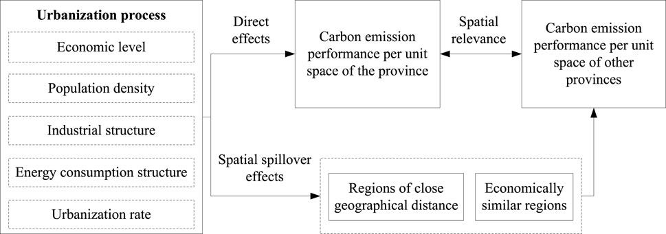
Figure 1. Theoretical framework of the impact of urbanization on carbon emission performance per unit space.
Using the carbon emission performance per unit space as the explanatory variable, the carbon emission is combined with GDP and built-up area, and the carbon emission effect of the city in the whole geographical space is considered, and the sustainability performance of different regions is compared. The provincial carbon emission data is derived from the Carbon Emission Accounts and Datasets (CEADs). The formula is as follows:
Where: CE is the total carbon emissions, Ck is the carbon emissions of fossil fuels, n is the type of fossil energy, ADi refers to the consumption of fossil fuels, and EFi is the emission coefficient of the fuel.
The formula for carbon emission performance per unit space is as follows:
where: Q(CO2)i,t represents the carbon emission performance per unit space of province i in year t, CEi,t represents the carbon emission of province i in year t, GDPi,t denotes the GDP of province i in year t, BUAi,t denotes the built-up area of province i in year t.
In this paper, the regression imputation method is used to deal with the missing values of the intermediate years. The average growth rate combined with adjacent time points was used to fill in the missing values of the years at both ends to improve the integrity and reliability of the data (Jin, 2001). Due to the differences in regional factors, historical development, industrialization and urbanization processes, if carbon emissions are only used as the explanatory variables, the error of the research results is large, and the conclusions do not have realistic reference value. In order to facilitate the study of the inter-regional carbon emission impact mechanism and draw the conclusion of effective emission reduction, the carbon emission performance per unit space was selected as the explanatory variable.
In this paper, economic level, population density, industrial structure, energy consumption structure, and urbanization rate are used as the criteria for measuring the urbanization process (Gan et al., 2011; Li et al., 2016; Shao et al., 2022). The definitions of indicators are shown in Table 1.
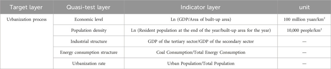
Table 1. Measurement system of urbanization process.
Due to the interdependence of economic activities at multiple levels such as trade, investment, and industrial chains, economic fluctuations or policy adjustments in one region often affect other regions, forming a strong macroeconomic correlation. At the same time, environmental protection policies and carbon emission reduction policies in various regions will have mutual influences, and regions tend to learn from and imitate each other, so macroeconomic variables such as carbon emissions have obvious spatial spillover effects. In this paper, a spatial Durbin model is constructed. The formula is as follows:
Where: k and j correspond to the cross-sectional units of each province; w is the element in the spatial weight matrix W; t represents the year; φ is the random perturbation term. lngdp is the vector of economic level variables; lnpop is the vector of population density; is the vector of industrial structure variables; es is the vector of energy consumption structure variables; urb is the vector of urbanization rate variables; X is the vector of other control variables.
Spatial autocorrelation is based on the spatial correlation measure, which describes and visualizes the spatial distribution pattern of things or phenomena to discover the degree of spatial agglomeration or dispersion, so as to reveal the spatial interaction mechanism between research objects (Gan et al., 2011). Spatial autocorrelation can be divided into global spatial autocorrelation and local spatial autocorrelation.
In the spatial econometric model, the weight matrix is exogenous, and the spatial weight matrix can be constructed as needed. In order to systematically investigate and flexibly respond to different spatial correlation patterns, so as to better understand the correlation between urban density and carbon emission performance per unit space, the following four spatial weight matrices are constructed, including geographic adjacency weight matrix, geographic distance weight matrix, economic distance weight matrix and economic geography weight matrix.
Geographic adjacency weight matrix: W1. It represents the connection between adjacent units in geographic space, for each geographic unit, the units directly adjacent to it are given a non-zero weight, and the units that are not directly adjacent are given a zero weight. The distance between regions i and j is expressed by dij, W1 = 1 when dij < d, and W1 = 0 when dij ≥ d.
Geo-distance weight matrix: W2. It represents the spatial distance relationship between geographic units, i.e., the reciprocal of the nearest road mileage between provinces. The surface distance of the provincial capital city calculated by latitude and longitude location is expressed by dij, W2ij = 0 when i = j, and W2ij = 1/dij when i≠j.
Economic distance weight matrix: W3. Due to the spatial correlation between the levels of regional economic development, in order to introduce more information of economic correlation and enhance the analysis of regional economic linkage, the weight matrix of economic distance with economic factors was constructed. The weights are the inverse of the difference in GDP between the two provinces. When i = j, Wij = 0. When i≠j, Wij = 1/|Yi-Yj|. Yi and Yj are the average regional GDP of province i and province j after GDP deflator processing from 2006 to 2021, respectively.
Economic Geography Weight Matrix: W4. Since the relationship between geography and economy may be nonlinear, relying only on geographical distance or economic distance to construct a matrix cannot fully capture the complex correlation between regions. The weight is the product of the difference in GDP between the two provinces and the reciprocal of the most recent road mileage between the two provinces. When i = j, Wij = 0. When i≠j, Wij = |Qi-Qj|/dij2. Qi and Qj are the mean regional GDP of province i and province j after GDP deflator processing from 2006 to 2021, respectively. dij2 is the square of the shortest road mileage between the two provinces. W4 takes into account both the proximity of geographical distance and the impact of economic activities on adjacent areas, which makes the understanding of the spatial correlation between cross-sectional units more comprehensive and accurate.
In order to investigate whether there is spatial autocorrelation in the whole spatial series, this paper uses the global Moran index to test the samples under each weight matrix. The global Moran index is shown below:
Where: xi is the carbon emission intensity per unit space of 29 provinces. S2 is the sample variance. wij is the (i,j) element of the spatial weight matrix. The Moran index ranges from −1 to 1. When the Moran index is close to 1 or −1, it means that there is an integer or negative spatial autocorrelation in the sample. When the Moran index is close to 0, it indicates that the spatial distribution is basically random, and there is no obvious trend of aggregation or dispersion. At the same time, it is also necessary to consider whether it is significant, and if it is significant, the null hypothesis that spatial autocorrelation does not exist is rejected, and it is believed that there is significant spatial autocorrelation between observations.
According to the results of the global spatial correlation test (Table 2), the Moran’s I index is significant under the weight matrix of W1, W2, W3 and W4, indicating that the distribution of carbon emission intensity per unit space shows spatial autocorrelation characteristics. There are not only spatial correlation characteristics of simple economic differences or geographical differences, but also comprehensive spatial correlation characteristics of geography and economy. In this paper, the empirical results of four weight matrices of W1, W2, W3 and W4 are used for spatial econometric analysis.
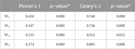
Table 2. Results of the global spatial correlation test of the weight matrix.
In this paper, 29 provincial-level administrative regions in China are taken as the research unit, including 22 provinces, four municipalities and 3 autonomous regions (Sun et al., 2015; Yang and zhang, 2024; Xu, 2024). Due to lack of data, the study area does not include Hong Kong, Macau, Taiwan, Xinjiang and Tibet. Based on the existing relevant literature, technological progress, openness to the outside world, building density, and environmental regulation were selected as the control variables in this paper (Zhang and Wei, 2014; An and Xie, 2015; Wei, 2017; SS et al., 2019). Technological progress is expressed as the inverse of energy intensity (Total energy consumption/GDP). The degree of openness to the outside world is expressed as the logarithm of the proportion of import and export trade volume in local GDP of each province. Building density refers to the ratio of the base area to the land area. The degree of environmental regulation is based on the proportion of environmental pollution control investment in each province to local GDP.
The GDP, population, output value of the secondary industry, output value of the tertiary industry, and investment in environmental pollution control are derived from the statistical yearbooks of each province and the statistical yearbook of China in each year. The population density, built-up area and urban area of the city are derived from China Urban Statistical Yearbook, China Urban and Rural Construction Statistical Yearbook, and China Urban Construction Statistical Yearbook. The total energy consumption and coal consumption are from China Energy Statistical Yearbook. Since the urban area data provided after 2006 in the China Urban Construction Statistical Yearbook is different from the city area data provided before 2006. In order to ensure the accuracy of the data, the time period of each indicator data is 2006–2021. The descriptive statistics of the indicator data are shown in Table 3.
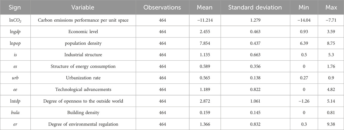
Table 3. Descriptive statistics of indicator data.
By comparing the mean, standard deviation, maximum, and minimum values of different variables, an initial understanding of their distribution and variability can be obtained. From the results of Table 1, it can be seen that the carbon emission performance per unit space varies greatly. Due to the differences in economy, technology, regional resources and other aspects, the carbon emission performance per unit space in different regions shows large differences. Among the explanatory variables, the difference in industrial structure is the most obvious, followed by population density, economic level and energy consumption structure, and the urbanization rate is the least different.
In order to better understand the annual trend and regional differences of carbon emission intensity per unit space, this paper divides the 29 provincial-level autonomous regions into four regions, namely, Eastern, Western, Central, and Northeastern, according to the interpretation of the National Development and Reform Commission, as shown in Table 4.
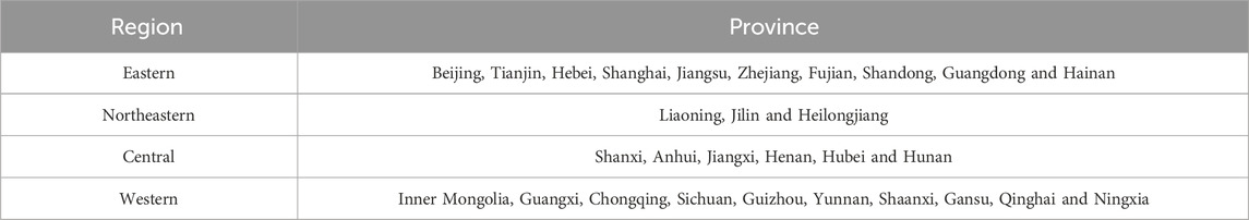
Table 4. Major provinces included in the four regions (Excluding Tibet, Xinjiang, Hong Kong, Macao and Taiwan).
According to Eqs 1 and 2, the carbon emissions of each region and the carbon emission performance per unit space in China are calculated. As can be seen from Table 5 (orange for the larger value and blue for the smaller value), China’s carbon emission performance per unit space is declining based on the time perspective. Except for the northeast, the east, west and central parts of the country showed a continuous downward trend, and the decline rate was about the same.
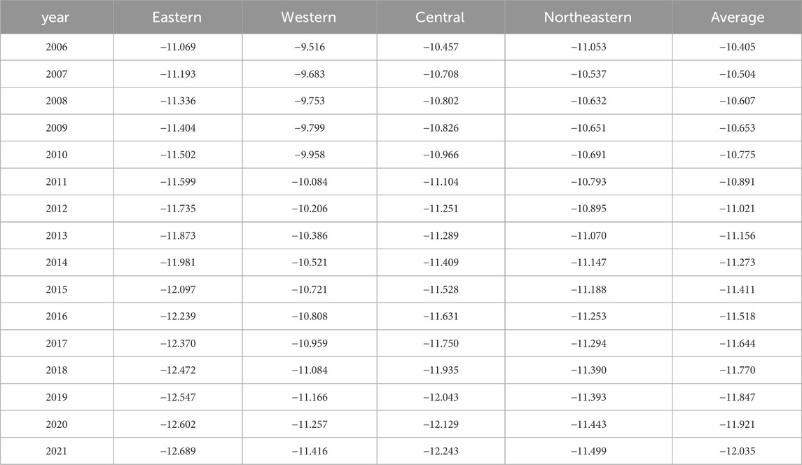
Table 5. Regional differences in carbon emission performance per unit space from 2006 to 2021.
With the increase of years, the Northeast region showed a trend of first increasing and then declining, reaching a peak in 2007 and then beginning to decline, and the decline rate was significantly lower than that in other regions. This is because China was in a relatively fast economic growth and high energy consumption in the early stage, which led to an increase in carbon performance. As the government’s attention to environmental sanitation continues to increase, a series of emission reduction measures have reduced carbon dioxide emissions. For example, in recent years, the western region has gradually formed a new pattern of large-scale protection, large-scale opening-up and high-quality development, so the carbon performance in the later period has shown a downward trend. From a spatial perspective, there are large regional differences in China’s carbon emission performance per unit space.
The lowest is in eastern China, including Beijing, Tianjin, Hebei, Shanghai, Jiangsu, Zhejiang, Fujian, Shandong, Guangdong and Hainan, followed by Northeast China, including Liaoning, Jilin and Heilongjiang, whose carbon emissions per unit space are roughly in the range of −11 to −13, all lower than the national average carbon emission performance per unit space. The carbon emission performance per unit space in the western region is higher than the national average. The performance of carbon emissions per unit space in the western provinces of Inner Mongolia, Guangxi, Chongqing, Sichuan, Guizhou, and Yunnan is about 1.35 times the national average.
The above phenomenon shows that the carbon emission performance per unit space is closely related to the level of economic development, energy consumption structure, industrial structure and other factors. The eastern region has a prosperous economy and a leading level of science and technology. The environmental capacity space is relatively sufficient, with advanced manufacturing and many cities with trillions of GDP. In particular, in recent years, China has accelerated its modernization and become a strategic highland in China’s science and technology, economy, and governance. However, due to the limitations of the geographical environment and ecological environment, the economic development level of the western region lags behind that of the eastern region. The technological level of environmental protection in the western region is relatively lagging behind, and there is a phenomenon of excessive exploitation of resources. As an economically underdeveloped and resource-endowed central region, its economic development has long relied on fossil fuels such as coal. In particular, in major coal provinces such as Shanxi and Henan, coal accounts for 80% and 76% of the energy consumption structure respectively, resulting in high carbon emissions.
As an important basis for distinguishing the traditional model from the spatial econometric model, the spatial correlation analysis can reduce the deviation in the measurement results. According to Eq. 4, 2), the global Moran’s I value and the corresponding p-value of each province from 2006 to 2021 can be obtained, as shown in Table 6.
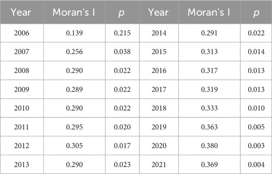
Table 6. Moran’s I value of carbon emission performance per unit space of Chinese provinces from 2006 to 2021.
As can be seen from Table 5, the Moran’s I value was below 0.05 in all years except 2006. Moran’s I values from 2007 to 2017 passed the test at the 5% significance level, and in all other years, the Moran’s I values passed the test at 1% significance. This indicates that the performance of carbon emissions per unit space of each province is not random, and there is a strong spatial positive correlation and a certain agglomeration effect. In other words, the provinces surrounding the provinces with high carbon emission performance per unit space also have high carbon emission performance per unit space, and the provinces with low carbon emission performance per unit space are clustered together. The performance level of carbon emission per unit space of each province is not only affected by its own economic activities, carbon production and consumption, but also by the carbon emissions, economic level, population density, industrial structure and other factors of surrounding provinces, such as the transfer of production activities, energy use diffusion, carbon trading market, etc.
The results of the global Moran index test show the overall situation of each province in terms of spatial carbon emissions, but cannot reflect the local spatial autocorrelation and spatial agglomeration of carbon emission performance per unit space, so the local Moran index is used for testing. The local Moran index formula is as follows:
Where: n is the total number of regions; yi is the carbon emission performance value per unit space of the 29 provinces;y is the average value of carbon emission performance per unit space, which is the (i,j) element of the spatial weight matrix.
According to Eq. 5, the Moran scatter plot is calculated and plotted. Moran scatter plots reflect the tendency of data to accumulate or disperse in space, and it divides observations into four quadrants.
First quadrant: High-High value agglomeration (HH) area. It indicates that the carbon emission performance per unit space of the observed provinces and their surroundings is high, showing a positive spatial correlation.
Second quadrant: Low-High value agglomeration (LH) region. It indicates that the carbon emission performance per unit space of the observed provinces is low, while the carbon emission performance per unit space of the surrounding provinces is high.
Third quadrant: Low- Low value agglomeration (LL) region. It indicates that the carbon emission performance per unit space of the observed province itself and its surroundings is low.
Fourth quadrant: high-low value agglomeration (HL) region. It indicates that the carbon emission performance per unit space of the observed provinces is high, while the performance per unit space of the surrounding provinces is low.
There is a positive correlation between the carbon emission performance per unit space in the first quadrant and the third quadrant. There is a negative correlation between the second quadrant and the fourth quadrant for carbon emission performance per unit space.
Based on the geographical adjacency weight matrix, the local Moran scatter plots for three representative years in 2006, 2014 and 2021 were drawn, as shown in Figure 2. The horizontal axis represents the standardized carbon emission performance value per unit space, and the vertical axis represents the spatial lag value of carbon emission performance per unit space. The figure shows that the carbon emission performance per unit space of most provinces is located in the HH and LL regions, that is, there is a positive spatial correlation. Specifically, in 2006, the provinces with HH carbon emission performance per unit space were Gansu, Ningxia, Shaanxi, Inner Mongolia, Yunnan, Shanxi, and Qinghai, which were concentrated in western China. The provinces located in the LL region include Hubei, Hunan, Anhui, Zhejiang, Shandong, Fujian, Jiangsu, Guangdong, Jiangxi, and most of them are concentrated in eastern China. In 2014, the number of HH regional provinces increased slightly, from 7 provinces in 2006 to 9, including Gansu, Ningxia, Inner Mongolia, Shaanxi, Shanxi, Hainan, Qinghai, Heilongjiang and Jilin. From 2006 to 2014, the concentration shifted from the western region to the western and northeastern regions. However, the number of LL-type provinces has changed little, from 9 districts in 2006 to 10 districts. The increase is in Guangxi, and the provinces are still concentrated in eastern China. In 2021, the HH-type region increased the number of Liaoning Province and the LL-type region increased the number of Yunnan Province, both of which were concentrated in the western, northeastern, and eastern parts of China, respectively, which were consistent with the results in 2014.
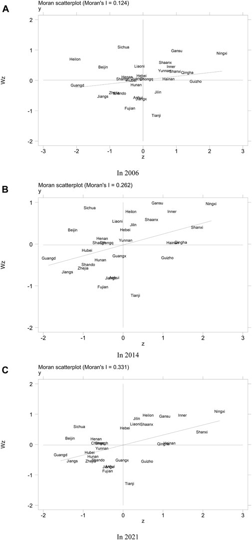
Figure 2. The performance of carbon emissions per unit space in 29 provinces in 2006 (A)-2014 (B)-2021 (C).
The above results are closely related to practical factors such as economic structure and industrial layout.
From a spatial perspective, most of the HH regions are provinces in the central and western regions. This is because the level of economic development in the central and western regions is limited and the level of urbanization is low. In addition, the western region, especially Shanxi, is more dependent on traditional energy sources, such as oil and coal, which makes the carbon emission performance per unit space of the provinces show a trend of high value agglomeration. The LL area is mostly in the eastern regions. Due to the relatively good level of economic development in the eastern region, it is easier to carry out industrial upgrading and technological innovation, and the level of urbanization is relatively high. At the same time, natural resources are relatively abundant, the climatic conditions are more suitable, and the energy utilization is more efficient. Therefore, the carbon emission performance per unit space of the provinces showed a trend of low value agglomeration. The phenomenon of high-value agglomeration in the eastern province and the low-value agglomeration in the western region are relatively stable, with strong path dependence.
From a time perspective, comparing the spatial agglomeration in 2006, 2014 and 2021, it can be seen that the number of low-value agglomeration provinces is increasing year by year, and is stable in the eastern region. The high-value agglomeration provinces are gradually concentrated in the western and northeastern regions from the western region. The number of provinces with low and high value agglomeration shows a decreasing trend year by year, while the number of provinces with high and low value agglomeration has been small or almost none.
Based on Eq. 3, a suitable spatial panel model is selected before exploring the spatial spillover effects of economic level, population density, industrial structure, energy consumption structure and urbanization rate on the performance of carbon emissions per unit space, so as to more accurately capture the possible spatial dependence and spatial spillover effects between variables. This paper uses the test idea of Elhorst (2014) to test the adaptability of the spatial panel model of the four weight matrices, and the results are shown in Table 7.
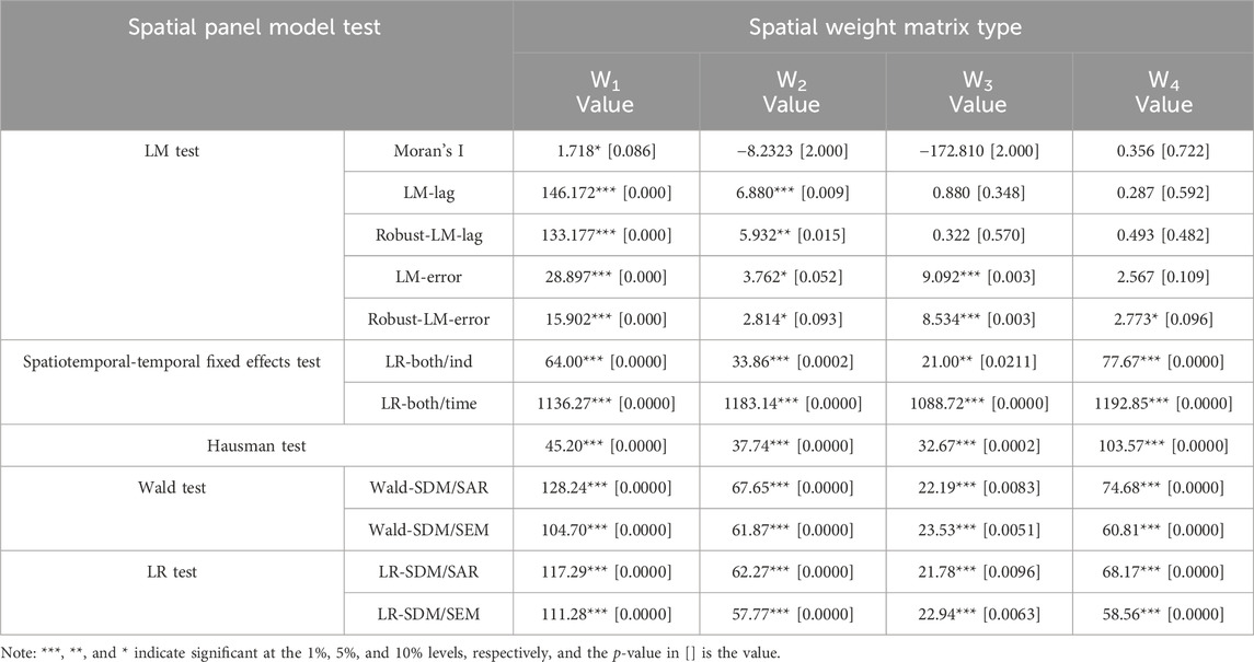
Table 7. Spatial panel model adaptation results.
The results show that when W1, W2, W3 and W4 weight matrices are used, the LM test statistics are significant, indicating that the choice of spatial econometric model is reasonable and the hybrid panel model is rejected. The spatial-temporal fixed-effect test of LR for W1, W2, and W4 all rejected the null hypothesis at the 1% level. The spatiotemporal fixed effect of W3 was significant at the 5% level and the temporal fixed effect was significant at the 1% level, indicating that the time-spatiotemporal double fixed effect model was more effective. The Hausman test of the four weight matrices was significant at the 1% level, which strongly rejected the null hypothesis and suggested that the fixed-effect model should be used. Both LR and Wald’s test were significant at the 1% level, indicating that the SDM model would not degenerate to the SEM model or the SAR model, and the SDM model was superior to the SEM model and the SAR model. Therefore, the spatial Durbin model with time-space-time double fixed effect is selected for analysis.
In order to better describe the interaction and dependence in geographic space, Stata was used to estimate the parameters of Equation 4 under the premise of considering spatial factors such as spatial correlation, spatial dependence, and spatial heterogeneity. The estimated results are shown in Table 8.
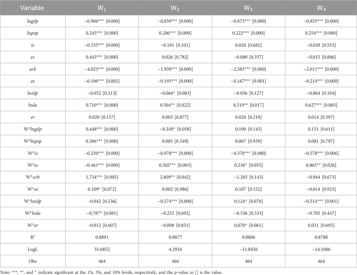
Table 8. Parameter estimation results.
As can be seen from Table 7, the values of R2 under different weight matrices are all greater than 0.87, indicating that the model fits well. On the whole, economic level, urbanization rate, technological progress, and openness to the outside world all have a negative impact on the carbon emission performance per unit space. Except for the degree of openness, it is significant at the level of 1%, and the degree of openness to the outside world is only significant at the level of 10% under the weight matrix of geographical distance. Population density, building density, and environmental regulation have a positive impact on the carbon emission performance per unit space. Population density is significant at the 1% level in all four matrices. However, the degree of environmental regulation has no significant impact on the carbon emission performance per unit space. In addition, the industrial structure and energy consumption structure have negative and positive effects on the carbon emission performance per unit space under the geographical adjacency matrix, respectively, and are significant at the 1% level, but fail the significance test in other matrices. The results of the study are as follows:
(1) Economic level. An increase in the economic level within a reasonable range can curb the increase in carbon emissions. With the development of the economy, the government has strengthened environmental awareness, enterprises have been transformed and upgraded, and cleaner and energy-saving technologies and equipment have been adopted to effectively reduce carbon emissions. However, the spatial lag term coefficient of the economic level is only significant in some spatial matrices, and some of the significance is not high. This indicates that the economic level of the province will have an impact on the carbon emission performance per unit space of neighboring provinces and geographically similar provinces, but the impact is not obvious.
(2) Population density. There is a positive correlation between population density and carbon emission intensity. It has a significant impact not only on the performance of carbon emissions per unit space of the local area, but also on the carbon emissions of neighboring regions. From the perspective of scale effect, areas with high population density have a larger scale of production, often have more enterprises and factories, and at the same time, regions need to provide more infrastructure services such as transportation, heating, and power supply, which increases overall energy consumption and carbon emissions. From the perspective of agglomeration effect, areas with high population density usually face more congested traffic, more intensive residential energy consumption, and relatively higher energy needs for residents’ lives, which in turn increases carbon emissions.
(3) Industrial structure. The regression coefficient of industrial structure to carbon emission performance per unit space is only significant at W1, but the spatial lag term coefficient is significantly negative under the four spatial matrices. This suggests that spatial proximity plays an important role in the impact between industrial structure and carbon emissions. Neighboring provinces and provinces with similar geographical distances have a strong interaction and similar economies have a significant agglomeration trend in terms of carbon emissions per unit space. With the adjustment and upgrading of industrial structure, economic development has gradually changed to the direction of high-tech and low-carbon, and the emergence of new high-tech industries, the support of green finance policies and a number of policy guidance have had a negative effect on the carbon emission performance per unit space.
(4) Energy consumption structure. The local energy consumption structure has a promoting effect on the carbon emission performance per unit space of the region and the economically similar regions. However, it has a restraining effect on carbon emissions in adjacent areas. China’s total energy consumption ranks among the top in the world, accounting for about 23% of the global total. Coal still accounts for a significant proportion of energy consumption, resulting in relatively high carbon emissions. Economically similar regions often have similar economic activities and industrial structures, and there is a certain supply and demand relationship. When local coal consumption increases, energy consumption in economically similar regions may also move in the same direction. However, due to the cross-regional balance between energy supply and demand, the surrounding areas will reduce their own coal consumption or adjust their energy structure, and stimulate technological progress and technology transfer, so that the carbon emission performance per unit space of the surrounding areas will be reduced.
(5) Urbanization rate. To a certain extent, strengthening urbanization has an inhibitory effect on the performance of carbon emissions per unit space. But too much aggregation will lead to a waste of resources. The spatial lag coefficient of urbanization rate was significantly positive in W1 and W2, and passed the test of significance of 1% and 5%, respectively. This indicates that the increase in local urbanization will have a promoting effect on carbon emissions in neighboring areas or areas with close geographical distances, but the effect is not obvious. As building traffic in cities becomes more compact and concentrated, energy losses in the transportation and supply process will gradually decrease, economic activities will become more concentrated, and resource utilization will be higher. At the same time, the mutual reinforcing effect between population and economic activity contributes to innovation and technological progress. However, due to the diffusion effect of economic activity, the number of businesses and residents in the periphery of the city has increased. This, in turn, creates more demand for energy consumption, which increases carbon emissions in the surrounding area.
For the other control variables, only technological progress and building density coefficient are significant in the four matrices, but they act in completely opposite directions. Technological progress can curb carbon emissions to a certain extent, and the increase in building density will increase carbon emissions. The spatial lag coefficients of technological progress, building density, openness to the outside world and environmental regulation are only significant in some matrices, indicating that the impact of these four variables on carbon emissions in the surrounding areas is not obvious.
In summary, economic level, industrial structure, and urbanization rate have a negative impact on carbon emissions. Population density and energy consumption structure have a positive impact on carbon emissions. The hypothesis H1 is demonstrated, that is, increasing the level of urbanization to a certain extent will reduce the carbon emission performance per unit space.
Due to the spatial spillover effect, the change of a variable will not only cause the change of carbon emission performance per unit space in the region, but also cause the change of carbon emission performance per unit space in adjacent areas. In order to accurately measure the influence of spatial effects on the relationship between variables, this paper will further decompose the impact of each variable on the performance of carbon emissions per unit space, including direct and indirect effects. Direct effects: the impact of a variable change on the carbon emission performance per unit space of the region, including the cyclic feedback effect of the variable change on the environmental factors in the surrounding neighboring areas and in turn the impact on the region. Indirect effects: the impact of a change of a variable on the performance of carbon emissions per unit space in adjacent areas and a series of chain reactions and adjustments, i.e., spatial spillover effects. In this paper, the model is decomposed according to the partial differential method, and the direct effects, indirect effects, and total effects of each variable under different weight matrices are obtained as shown in Table 9.
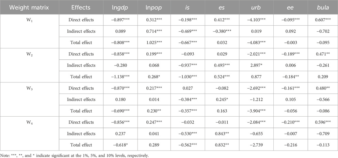
Table 9. Decomposition results of spatial effects.
Since the coefficients of the degree of openness to the outside world and the degree of environmental regulation are not significant, the spatial effect is not statistically significant, so it is not discussed here.
Overall, the total effect of the four weight matrices is basically the same. The direct effects of the geographic adjacency matrix and the geographic distance matrix affect the same direction. However, there are some differences in the direction of the direct effects of the economic distance matrix and the economic geography matrix. This is because economic factors are introduced into these two matrices, and China has a vast territory, there are obvious differences in economic development between regions, and it is affected by many factors such as history, culture, and policy, so there are differences in the direction of influence. At the same time, there are certain differences in the direction of the indirect effects of the four weight matrices. This is due to the fact that there are obvious spatial externalities in China’s economic and social activities. Moreover, the inter-regional connection network is very complex, including transportation, population flow, industrial chain and other contact methods between cities, and the interaction of multiple effects leads to the diversification of indirect effects.
At the specific level, the direct effects of economic level, population density and urbanization rate under the four matrices all passed the significance test of 1%. However, the indirect effect is only significant in some matrices. This indicates that these three factors have a certain spatial spillover effect, but it is not obvious. The indirect effects of industrial structure and energy consumption structure are significant. However, the direct effect was only significant in W1. This indicates that the impact of industrial structure and energy consumption structure on carbon emissions in geographically adjacent or economically similar regions is more significant than that on this region.
In the energy consumption structure, the order of the coefficient of indirect effect estimation of each matrix is as follows: W4(0.843)>W2(0.495)>W1(-0.380)>W3(0.245). This reflects that among the spillover factors that affect the carbon emission performance per unit space of energy consumption structure, economic geographic nesting is the main factor, and proximity is a secondary factor. This may be due to the impact of the dual carbon policy, which is prone to strategic competition among regions. Therefore, it is necessary to strengthen cooperation, consultation and experience sharing when formulating emission reduction policies to achieve greater emission reduction benefits.
Among the control variables, although the direct effects of technological progress and building density are significant in the four matrices, the total effects are only significant in some matrices, indicating that although the introduction of new technologies can reduce the carbon emission intensity of buildings, transportation and industry. But it may lead to more resource consumption and environmental pollution. Increased building density helps reduce commuting distances and traffic demands. However, it may lead to higher energy consumption. The combined effects of the two cancel each other out to a certain extent, resulting in insignificant results.
In summary, economic level, population density, industrial structure, energy consumption structure, and urbanization rate all have spatial spillover effects. That is, there is a spatial spillover effect of urbanization process on the carbon emission performance per unit space of neighboring provinces, and hypothesis H2 is demonstrated.
In order to further verify the robustness of the model, this paper uses the method of substituting explanatory variables to test. Drawing on the research ideas of Cheng et al. (2013) and Liu and Liu (2021), the per capita GDP is used to represent the economic level, and the proportion of the output value of the secondary industry in the GDP represents the industrial structure, and the model regression is carried out after substituting the explanatory variables. The regression results are shown in Table 10. The results show that there is no significant change in the main regression results, indicating that the test in this paper is robust.
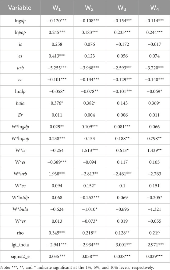
Table 10. Robustness test results.
Based on the consideration of multiple spatial factors, this paper conducts a new empirical analysis of the regional differences, spatial autocorrelation, and spatial effects of carbon emission performance per unit space. This paper studies whether promoting urbanization can help achieve the goals of carbon neutrality and carbon peaking.
(1) To a certain extent, increasing the level of urbanization will reduce the carbon emission performance per unit space. Population density has a significant effect on the performance of carbon emissions per unit space in both local and adjacent areas. Spatial proximity plays an important role in the impact between industrial structure and carbon emissions. The energy consumption structure has a promoting effect on the carbon emission performance per unit space in local and economically similar regions, but has a restraining effect on the carbon emissions in adjacent areas. From 2006 to 2021, China’s carbon emission performance per unit space showed a downward trend year by year. The decline rate was similar in the east, west and central part of the country, with the northeast rising first and then decreasing. In terms of intensity, the eastern part is the lowest, followed by the central and northeastern regions, and the western part is the highest. The level of economic development, energy consumption structure, and industrial structure are closely related to the carbon emission performance per unit space.
(2) The urbanization process has a spatial spillover effect on the carbon emission performance per unit space of neighboring provinces. Among them, the spatial spillover effects of industrial structure and energy consumption structure are more obvious than those of economic level, population density and urbanization rate. Economic geographic nesting is the main factor that affects the spillover of energy consumption structure on carbon emission performance per unit space. There is a strong positive correlation and stable path dependence on the performance of carbon emissions per unit space in each region. The number of LL agglomeration provinces is increasing year by year, and it is stable in the eastern region. The HH agglomeration provinces are gradually concentrated in the western and northeastern regions from the western region. There are few LH agglomeration provinces and HL agglomeration provinces, which show a decreasing trend year by year.
Based on the research conclusions of this paper, such as the impact of urbanization level on carbon emission performance per unit space and the spatial spillover effect, some policy suggestions are put forward for urban development.
(1) Strengthen the management of carbon emissions in densely populated areas and adjacent areas. Focus on public transportation, energy-saving buildings and green space construction, and promote low-carbon production and clean energy utilization. Strengthen the formulation and enforcement of environmental protection laws and regulations, and impose restrictions and penalties on enterprises with high carbon emissions.
(2) Promote the upgrading and optimization of industrial structure and strengthen regional cooperation. Due to the important role of spatial proximity, the government needs to continue to promote technological innovation in the process of industrial restructuring and upgrading. Realize the withdrawal of old production capacity and the construction of new production capacity. Strengthen inter-regional industrial ties and economic cooperation to promote the further reduction of carbon emissions.
(3) Adjust the energy consumption structure and promote the transformation of the energy consumption structure to clean energy. Increase investment in R&D and promotion of clean energy technologies, and encourage enterprises and residents to use clean energy. At the same time, preferential policies such as loan support and tax incentives are provided to promote the development and application of clean energy.
(4) Strengthen cross-regional cooperation mechanisms, such as building a cross-regional environmental protection information platform to share environmental protection management experience, monitoring data and technological achievements. Promote experience sharing and technology transfer to achieve greater carbon emission reduction and environmental protection benefits.
The original contributions presented in the study are included in the article/Supplementary Material, further inquiries can be directed to the corresponding author.
YY: Methodology, Supervision, Writing–review and editing, ZJ: Formal Analysis, Software, Writing–original draft, HJ: Data curation, Writing–review and editing. KX: Investigation, Resources, Writing–review and editing.
The author(s) declare that financial support was received for the research, authorship, and/or publication of this article. This work was supported by the Key Project of Beijing Social Science Foundation (Project No. 19YJA001).
The authors declare that the research was conducted in the absence of any commercial or financial relationships that could be construed as a potential conflict of interest.
All claims expressed in this article are solely those of the authors and do not necessarily represent those of their affiliated organizations, or those of the publisher, the editors and the reviewers. Any product that may be evaluated in this article, or claim that may be made by its manufacturer, is not guaranteed or endorsed by the publisher.
An, C., and Xie, J. (2015). Research on the relationship between carbon dioxide emissions, energy intensity and economic growth. J. Commer. Econ. (15), 38–39.
Chen, C. C., Liu, C. L., and Wang, H. (2014). Examining the impact factors of energy consumption related carbon footprints using the STIRPAT model and PLS model in Beijing. China Environ. Sci. 34 (6), 1622–1632. doi:10.1016/j.apenergy.2013.01.036
Cheng, Y. Q., Wang, Z. Y., and Zhang, S. Z. (2013). Spatial econometric analysis of carbon emission intensity and its driving factors from energy consumption in China. Acta Geogr. Sin. 68 (10), 1418–1431.
Daly, H. E. (1974). The world dynamics of economic growth:the economics of the steady state. Am. Econ. Rev. 64 (2), 15–23.
Du, H. B., Li, N., and Wang, Y. Y. (2013). Study on China’s carbon emission performance and influencing factors from the perspective of spatial economics. J. Tianjin Univ. Soc. Sci. 15 (05), 411–416.
Elhorst, J. P. (2014). Matlab software for spatial panels. Int. Regional Sci. Rev. 37 (3), 389–405. doi:10.1177/0160017612452429
Ewing, R., and Rong, F. (2008). The impact of urban form on U.S. residential energy use. Hous. Policy Debate 19 (1), 1–30. doi:10.1080/10511482.2008.9521624
Feng, R. (2011). Study on the methods and application of estimation of CO2 emission on urban household energy consumption [D]. Nankai University
Fu, S., and Fu, B. (2019). Concept clarification of eco-geography and analysis of related classical studies. Scien. Geogra. Sinica. 39 (1), 70–79. doi:10.13249/j.cnki.sgs.2019.01.008
Gan, C. H., Zheng, R. G., and Yu, D. F. (2011). An empirical study on the effects of industrial structure on economic growth and fluctuations in China. Econ. Res. J. 46 (05), 4–16+31.
Hilber, C. A. L., and Palmer, C. (2014). Urban development and air pollution: evidence from a global panel of cities. Social Science Electronic Publishing. doi:10.2139/ssrn.2541387
Hu, C. Z., Huang, X. J., and Zhong, T. Y. (2008). Characteristics of carbon emission in China and analysis on its cause. China Popul. Resour. Environ. 18 (03), 38–42. doi:10.1016/s1872-583x(09)60006-1
Hua, J., Ren, J., and Xu, M. (2013). Evaluation of Chinese regional carbon dioxide emissions performance based on a three-stage DEA model. Resour. Sci. 35 (07), 1447–1454.
Ishii, S., Tabushi, S., Aramaki, T., and Hanaki, K. (2009). Impact of future urban form on the potential to reduce greenhouse gas emissions from residential, commercial and public buildings in Utsunomiya, Japan. Energy Policy 38 (9), 4888–4896. doi:10.1016/j.enpol.2009.08.022
Jin, Y. J. (2001). Imputation adjustment method for missing data. J. Appl. Statistics Manag. (06), 47–53. doi:10.13860/j.cnki.sltj.2001.06.012
Jing, Q. N., Hou, H. M., and Bai, H. T. (2019). A top-bottom estimation method for city-level energy-related CO2 emissions. China Environ. Sci. 39 (01), 420–427. doi:10.19674/j.cnki.issn1000-6923.2019.0052
Li, J., and Zhou, H. (2012). Correlation analysis of carbon emission intensity and industrial structure in China. China Popul. Resour. Environ. 22 (01), 7–14.
Li, X. P., Wang, S. B., and Hao, L. L. (2016). Environmental regulation, innovation-driven and inter-provincial carbon productivity changes in China. J. China Univ. Geosciences Soc. Sci. Ed. 16 (01), 44–54.
Liang, Q. (2005). Spatial economy: past, present future -in review of the spatial economy: cities, regions and international trade. China Econ. Q. (03), 1067–1086.
Lin, B. Q., and Liu, X. Y. (2010). China’s carbon dioxide emissions under the urbanization process: influence factors and abatement policies. Econ. Res. J. 45 (08), 66–78.
Liu, G. P., and Zhu, D. J. (2013). Research on provincial wellbeing performance of carbon emissions in China. Account. Econ. Res. 27 (06), 74–81.
Liu, X. B, and Liu, Q. M. (2021). Study on the relationship between economic growth, urbanization and carbon dioxide emission intensity from spatial perspective. J. Commer. Econ. (12), 184–188.
Ou, J., Liu, X., Li, X., and Chen, Y. (2013). Quantifying the relationship between urban forms and carbon emissions using panel data analysis. Landsc. Ecol. 28 (10), 1889–1907. doi:10.1007/s10980-013-9943-4
Shao, S., Fan, M. T., Yang, L. L., and Restructuring, E. (2022). Green technical progress, and low-carbon transition development in China: an empirical investigation based on the overall technology frontier and spatial spillover effect. J. Manag. World 38 (02), 46–69+4-10. doi:10.19744/j.cnki.11-1235/f.2022.0031
Shao, S., Zhang, K., and Dou, J. M. (2019). Effects of economic agglomeration on energy saving and emission reduction: theory and empirical evidence from China. J. Manag. World 35 (01), 36–60+226. doi:10.19744/j.cnki.11-1235/f.2019.0005
Shen, Y. F., Shi, X. P., Zhao, Z. B., Sun, Y. P., and Shan, Y. L. (2023). Measuring the low-carbon energy transition in Chinese cities. iScience 26 (01), 105803. doi:10.1016/j.isci.2022.105803
Song, D. Y., and Lu, Z. B. (2009). The factor decomposition and periodic fluctuations of carbon emission in China. China Popul. Resour. Environ. 19 (03), 18–24.
SS, H., and Zhu, X. A. (2019). Spatial econometrics for influencing factors of regional green development of China. Econ. Surv. 36 (01), 10–17. doi:10.15931/j.cnki.1006-1096.20181213.011
Sun, C. L., Jin, N., and Zhang, X. L. (2013). The impact of urbanization on the CO2 emission in the various development stages. Sci. Geogr. Sin. 33 (03), 266–272. doi:10.13249/j.cnki.sgs.2013.03.006
Sun, H., Liang, H. M., and Chang, X. L. (2015). Land use patterns on carbon emission and spatial association in China. Econ. Geogr. 35 (03), 154–162. doi:10.15957/j.cnki.jjdl.2015.03.023
Sun, M. (2010). Empirical study on the effects of China’s energy consumption and carbon emissions changes. Jilin University.
Wang, D. (2012). Study on calculation and carbon emission reduction approaches in Chinese residents’ consumption in the process of urbanization. Nankai University.
Wei, G. Q. (2017). Study on the influence of population structure change and consumption pattern on carbon emission. J. Commer. Econ. (16), 37–39.
Xu, X. (2024). Multidimensional measurement, spatial differences and dynamic evolution of high-quality development of new-type urbanization. Statistics Decis. 40 (10), 100–105.
Yan, W. T., Xiao, J. H., and Hu, H. (2012). Urban spatial structure and environmental performance: review and thought. Urban Plan. Forum (05), 50–59.
Yang, C. Y., and Zhang, N. (2024). Research on the heterogeneous consumption effect of urbanization under different development models: based on the observation perspective of human urbanization and urbanization of production factors. J. Commer. Econ. (11), 60–63.
Zahabi, S. A. H., Miranda-Moreno, L., Patterson, Z., Barla, P., and Harding, C. (2012). Transportation greenhouse gas emissions and its relationship with urban form, transit accessibility and emerging green technologies: A Montreal case study. Procedia - Soc. Behav. Sci. 54 (2375), 966–978. doi:10.1016/j.sbspro.2012.09.812
Zhang, H., and Wei, X. P. (2014). Green paradox or forced emission-reduction: dual effect of environmental regulation on carbon emissions. China Popul. Resour. Environ. 24 (09), 21–29.
Zhang, T. F., Yang, J., and Sheng, P. F. (2016). The impacts and channels of urbanization on carbon dioxide emissions in China. China Popul. Resour. Environ. 26 (02), 47–57.
Zheng, C. D., and Liu, S. (2011). Industrial structure and carbon emissions: an empirical analysis based on inter-provincial panel data in China. Res. Dev. (02), 26–33. doi:10.13483/j.cnki.kfyj.2011.02.013
Zhu, Q., Peng, X. Z., and Lu, Z. M. (2010). Analysis model and empirical study of impacts from population and consumption on carbon emissions. China Popul. Resour. Environ. 20 (02), 98–102.
Zhuang, G. Y. (2021). Challenges and countermeasures for China to achieve the "dual carbon" goal. People’s Trib. (18), 50–53.
Keywords: urbanization, carbon emissions, carbon performance, spatial Dubin model, spatial spillover environment performance
Citation: Jianmin Z, Yang Y, Jingyuan H and Xiaoxuan K (2024) Can urbanization improve carbon performance?. Front. Environ. Sci. 12:1431324. doi: 10.3389/fenvs.2024.1431324
Received: 11 May 2024; Accepted: 24 June 2024;
Published: 15 July 2024.
Edited by:
Mariarosaria Lombardi, University of Foggia, ItalyReviewed by:
Gianluigi De Pascale, University of Foggia, ItalyCopyright © 2024 Jianmin, Yang, Jingyuan and Xiaoxuan. This is an open-access article distributed under the terms of the Creative Commons Attribution License (CC BY). The use, distribution or reproduction in other forums is permitted, provided the original author(s) and the copyright owner(s) are credited and that the original publication in this journal is cited, in accordance with accepted academic practice. No use, distribution or reproduction is permitted which does not comply with these terms.
*Correspondence: Yang Yang, Ynd1X3lhbmd5YW5nQDEyNi5jb20=
Disclaimer: All claims expressed in this article are solely those of the authors and do not necessarily represent those of their affiliated organizations, or those of the publisher, the editors and the reviewers. Any product that may be evaluated in this article or claim that may be made by its manufacturer is not guaranteed or endorsed by the publisher.
Research integrity at Frontiers
Learn more about the work of our research integrity team to safeguard the quality of each article we publish.