Air pollution prediction using blind source separation with Greylag Goose Optimization algorithm

Particularly, environmental pollution, such as air pollution, is still a significant issue of concern all over the world and thus requires the identification of good models for prediction to enable management. Blind Source Separation (BSS), Copula functions, and Long Short-Term Memory (LSTM) network integrated with the Greylag Goose Optimization (GGO) algorithm have been adopted in this research work to improve air pollution forecasting. The proposed model involves preprocessed data from the urban air quality monitoring dataset containing complete environmental and pollutant data. The application of Noise Reduction and Isolation techniques involves the use of methods such as Blind Source Separation (BSS). Using copula functions affords an even better estimate of the dependence structure between the variables. Both the BSS and Copula parameters are then estimated using GGO, which notably enhances the performance of these parameters. Finally, the air pollution levels are forecasted using a time series employing LSTM networks optimized by GGO. The results reveal that GGO-LSTM optimization exhibits the lowest mean squared error (MSE) compared to other optimization methods of the proposed model. The results underscore that certain aspects, such as noise reduction, dependence modeling and optimization of parameters, provide much insight into air quality. Hence, this integrated framework enables a proper approach to monitoring the environment by offering planners and policymakers information to help in articulating efficient environment air quality management strategies.

1 Introduction

Reduced accessibility to fresh air due to accelerated urbanization and the boom of the industrial sector prominently worsen the alarming problem of air pollution (Ravindra et al., 2019). These changes are more visible due to the emergence of urban areas and the establishment of new industrial plants. Appropriately tracking and predicting air pollution levels during a turning point is both a scientific challenge and an emergency need for environmental health and stability (Asamoah et al., 2020). Within this environment, the Air Quality Monitoring Dataset acts as a helpful information source, combining sensor data, weather data, and statistics on air pollution. Nevertheless, the natural power of the dataset is hidden beneath the continuous antagonizing noise—an opponent that has the power to interfere with the precision of the air pollution forecast (Al-Janabi et al., 2020). To tackle this issue, a range of advanced statistical measures are introduced, for instance, Blind Source Separation (BSS), Principal Component Analysis (PCA), Independent Component Analysis (ICA), and cluster optimization to produce well-balanced assimilation of data and contribute to the improvement of the air pollution prediction process (Pion-Tonachini et al., 2019; Ma and Zhang, 2021; Chang et al., 2022; Greenacre et al., 2022).

Environmental monitoring becomes vital and infinitive to the work, going beyond the factual evidence already used. The significance of environmental monitoring in the context of air pollution has gained broad acceptance, such that further steps can be implemented based on the data produced (Jiang et al., 2020). This anticipatory piece is the weapon to protect human health from threats and to prevent the imbalance in ecology. In addition to improving environmental monitoring processes, the paper also explores the details underlying the tightly-knit relationship between air pollution and environmental variables (Jafarzadegan et al., 2019; Mengist et al., 2020).

Our paper relies on such BSS methods as PCA and ICA as their most recognizable tools (Monakhova and Rutledge, 2020; Yang et al., 2021). Incorporating the principal component analysis into its dimensionality reduction techniques, PCA can map out the critical constituents of the dataset. ICA goes beyond PCA in this aspect since it works with components that show the complex nature of mixed data, providing more independence. The synergistic use of these methods makes the signals and the noise decompose in a more aligned way. Therefore, the depth of comprehension of the processes dictating air pollution was offered (Rizk et al., 2023).

We illustrate an analogy of noise as a puzzle and discuss how cluster optimization is an all-embracing solution. Knowing that noise in a dataset often forms clusters, cluster optimization lets us focus on the noise sources near one another. This leveling-up helps generate high-quality data and betters the accuracy of forecasts, bypassing paperwork and focusing on noise mitigation with impact precision (Rizk et al., 2024).

Consequently, the paper endeavors to address the following paper questions:

1. How effective are Blind Source Separation (BSS) techniques in isolating independent sources of air pollution from the mixed sensor data?

2. Can the Greylag Goose Optimization (GGO) algorithm significantly enhance the performance of BSS methods and improve the accuracy of air quality predictions?

3. How well do Copula functions model the dependence structure between different environmental and pollutant variables to enhance prediction accuracy?

4. What is the comparative performance of GGO-optimized Long Short-Term Memory (LSTM) networks in forecasting carbon monoxide (CO) concentrations, compared to other optimization techniques?

5. Does the predictive model maintain high accuracy across different temporal and meteorological scenarios, ensuring robust air quality forecasts?

The subsequent sections delve into the methodologies and techniques employed in this study. They begin with a detailed description of the dataset, emphasizing the environmental and pollutant parameters measured. Data preprocessing steps, including normalization, feature selection, and handling of missing data, are then discussed.

Following this, the paper explores Blind Source Separation (BSS) methods like Principal Component Analysis (PCA) and Independent Component Analysis (ICA), explaining their role in noise reduction and source isolation. The use of Copula functions to model dependence structures between variables is also examined.

The optimization of BSS and Copula parameters using the Greylag Goose Optimization (GGO) algorithm is detailed, highlighting its impact on model performance. The application of Long Short-Term Memory (LSTM) networks for predicting carbon monoxide (CO) concentrations, optimized by GGO, is then presented.

The evaluation section compares the GGO-LSTM model’s performance with other techniques across various metrics. The paper concludes with insights into the findings, the model’s robustness, and recommendations for future research and policy-making in air quality management.

2 Related works

An exhaustive Table 1 elucidates the demonstration of involvement, encapsulating diverse inquiries within the realm of BSS enhancement for effective environmental monitoring.

Table 1

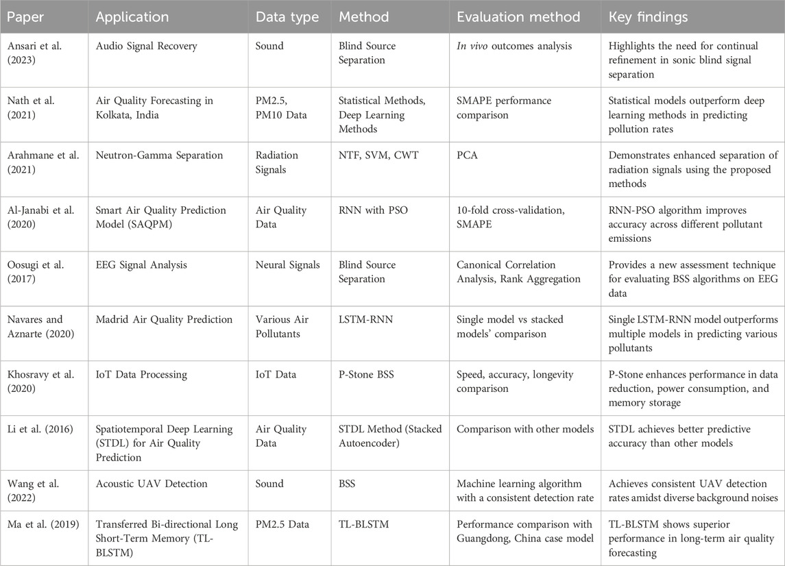
Table 1. Summary of related works for the prediction of student’s academic performance.

When these scholarly contributions are aggregated, it becomes evident that there is a pressing need to enhance the precision of Separation techniques for identifying air pollution across diverse domains. These studies pivot on distinctions in data types, methodologies, and measurements, offering a comprehensive perspective on viable security solutions.

3 Materials and methods

This paper’s material and methods show the complicated processes and methods that deal with the robustness issue in noise-plagued air pollution datasets. A practical approach to improving the accuracy of predictive models is to be equipped with a complete grasp of the tools and techniques used.

3.1 Copula

A copula function is a mathematical tool in probability theory and statistics that provides a mathematical framework for relating random variables despite the entirely different characteristics of their distributions (Zaki et al., 2023a). In a nutshell, it sketches how variables give rise to interdependence or correlation without considering the separate distribution of variables. These copula functions not only participate in different fields such as multivariate analysis, risk management, finance, and reliability engineering but also understand and model the relations structure of variables, which plays a critical role in each of these disciplines. The copula is sparse, which helps us describe a multivariate distribution with a dependent structure (Razmkhah et al., 2022). Nelsen (2007) introduced copulas as follows: a copula is a function that joins multivariate distribution functions with uniform [0, 1] margins.

Theorem 1. (Sklar theorem) Sklar (1973) considers the two random variables X and Y, with distribution functions F(x) and F(y), respectively, then the CDF and PDF for bivariate copula are respectively given as:

$F\left(x,y\right)=F\left(x,y\right)=C\left(F\left(x\right),F\left(y\right)\right),$

$f\left(x,y\right)=f\left(x\right)f\left(y\right)c\left(F\left(x\right),F\left(y\right)\right).$

The Gaussian copula is a popular and widely used method of constructing multivariate distributions that models joint dependence for random variables. It works based on the metric that the separate distributions of the variables are jointly normal, and it uses the copula function to describe their collective distribution. Through this approach, dependencies between variables that need to be captured and understood are separated from the process of creating single-variable distributions, thus providing better results in finance, risk management, and in their goals like comprehending and modeling interdependence between variables (Xiao et al., 2022).

Unlike the Gaussian copula, the PDF and CDF generally do not have a closed form in their expression. Nonetheless, for the conditional distributions of the Gaussian (standard) type, and when the correlation matrix is known, the joint distribution is calculated via the multivariate Gaussian distribution (Chen et al., 2020).

Let’s denote $\left(F_i\left(x_i\right)\right)$ as the CDF of the $\left(i\right)-$ th variable, and $\left(\mathrm{\Phi }\right)$ As the cumulative distribution function of the standard normal distribution. The joint cumulative distribution function of the Gaussian copula is given by:

$C\left(u,\rho \right)={\mathrm{\Phi }}_{\rho }\left({\mathrm{\Phi }}^{-1}\left(u_1\right),{\mathrm{\Phi }}^{-1}\left(u_2\right),\dots ,{\mathrm{\Phi }}^{-1}\left(u_n\right)\right)$

where $\left(u_i=F_i\left(x_i\right)\right)$ Are the marginal cumulative probabilities and $\left(\rho \right)$ Is the correlation matrix.

The PDF of the Gaussian copula is found by taking the derivative of the multivariate cumulative distribution function. Nevertheless, this exchange form is rather complicated and is usually not used because it is too complex.

3.2 Principal component analysis (PCA)

PCA is one of the most applied statistical methods for reducing the dimensionality and regaining understanding of the acquired data (Libório et al., 2022). It aims to transform the original data into a new dataset composed of powerful uncorrelated variables called principal components, which take the maximum variance from the data. The PCA does this by identifying the directions (principal axes) along which the data varies the most, leading to a reduced dimensionality of data representation.

PCA is based on linear algebra concepts, and the computational procedure consists of calculating eigenvectors and eigenvalues from the covariance matrix of the original data. The mathematical foundation can be expressed through the following equations: The mathematical foundation can be expressed through the following equations:

$\text{Covariance\hspace{0.17em}matrix }C=\frac{1}{m-1}{\left(X-\overline{X}\right)}^T\left(X-\overline{X}\right)$

where $X$ is the data matrix with dimensions $m\times n$ (where $m$ is the number of observations and $n$ is the number of variables), and $\overline{X}$ is the mean of each variable (Kherif and Latypova, 2020; Kahl et al., 2021).

Compute Eigenvectors and Eigenvalues: $C\cdot \text{eigenvector}=\text{eigenvalue}\cdot \text{eigenvector}$

The eigenvectors represent the principal components, and the corresponding eigenvalues indicate the variance each component captures. Sort the eigenvalues in descending order and select the top $k$ eigenvectors to form the matrix $W_k$, representing the transformation matrix.

Transform Original Data: $\text{Transformed\hspace{0.17em}data }Y=X\cdot W_k$

3.3 Blind source separation (BSS)

BSS is a powerful signal processing technique designed to unveil independent source signals from observed mixtures without prior knowledge of the sources or the mixing process (Sawada et al., 2019; Yang et al., 2019). In air pollution paper, where pollutant concentrations arise from various sources with complex interactions, BSS is a valuable tool for uncovering the underlying dynamics. The fundamental principle involves the assumption that the observed data matrix ($\mathbf{X}$) can be represented as the product of a mixing matrix ($\mathbf{A}$) and an independent source matrix ($\mathbf{S}$):

$\mathbf{X}=\mathbf{AS}$

Each column of $\mathbf{S}$ corresponds to an independent source signal, and each column of $\mathbf{X}$ represents the observed mixture. The challenge is to estimate $\mathbf{S}$ by inversely solving the mixing process, revealing the underlying independent sources contributing to the observed data.

The mathematical foundation of BSS often relies on ICA, a widely used technique. The observed data matrix $\mathbf{X}$ is assumed to be a linear combination of independent source signals, and the goal is to find a demixing matrix ($\mathbf{W}$) such that $\mathbf{S}=\text{WX}$. This process involves maximizing the statistical independence of the estimated sources. The estimated independent sources (${\mathbf{S}}_{\text{est}}$) can be expressed as:

${\mathbf{S}}_{\text{est}}=\mathbf{WX}$

ICA algorithms, including Fast ICA, Joint Approximate Diagonalization of Eigen-matrices (JADE), and Infomax, iteratively adjust the demising matrix to achieve the separation of sources.

Figure 1 illustrates the fundamental concept of BSS, a signal processing technique designed to untangle mixed signals without prior knowledge of the sources or the mixing process. This visualization provides an insightful overview of the BSS process, showcasing how the algorithm disentangles the source signals from their mixed counterparts.

Figure 1

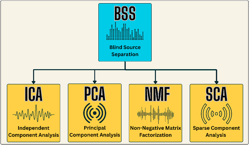
Figure 1. The blind sources separation (BSS).

3.4 Long short-term memory (LSTM)

LSTM is a Recurrent Neural Network (RNN) type that can be selected for time-series prediction applications, including air pollution because it efficiently analyzes long-term temporal patterns in data. LSTM networks use memory cells and gates to control the flow of information and are, therefore, capable of retaining information over a sequence period. When they are all connected, these are the input gate, the forget gate, the output gate, and the cell state, which are responsible for deciding when to retain and discard information.

Thus, prior to applying LSTM to predict air pollution, the input values are normalized to scale the input features to values between 0 and 1. This is then followed by the sliding window approach, which creates subsequences of the input data and the corresponding target outputs. The dataset is divided into training and test sets to assess the model’s ability to generalize to data it has not seen during training (Chang et al., 2020).

Starting with initial weights and bias and after passing the Input sequences through the LSTM network to get the predictions, the Loss can be computed using a loss function such as MSE, which represents the differences between the actual and predicted values and weights/biases can be tuned through backpropagation through time (BPTT). Stochastic gradient descent or its modifications like Adam or RMSprop are used to make incremental changes to the model parameters. To measure the accuracy of the LSTM model, MAE, RMSE, and R2 statistical measures are used, which determine the accuracy and the amount of variance in the model explained. Being a form of recurrent neural network, LSTM networks can meet the data’s temporal processing requirements and are appropriate for predicting the concentrations of pollutants.

3.5 Greylag Goose Optimization (GGO) algorithm

The best way to develop the BSS with the help of GGO is demonstrated in the paper regarding environmental cleanup and particularly noise reduction (Szipl et al., 2019; Hoarau et al., 2022; Zaki et al., 2023b). This part describes the complete recommendation on how GGO can tune BSS parameters and optimize LSTM hyperparameters.

3.5.1 GGO algorithm

The GGO algorithm starts by creating individuals that randomly generate candidate solutions to the problem. Each individual represents such candidate solutions. The term GGO ($X_i$, i = 1,2,…,n) stands for the population of the group, n, with an integer denoting the size of the population (Dokeroglu et al., 2019; Braik et al., 2021).

In Figure 2, we delve into the exploration and exploitation dynamics of the GGO algorithm. This visualization captures the essence of GGO as it navigates the solution space, striking a balance between exploration (searching for new, potentially better solutions) and exploitation (refining known solutions). The figure features a dynamic representation of GGO’s iterative process, emphasizing how the algorithm optimally combines exploration and exploitation strategies to achieve efficient and effective solutions (Halim et al., 2021).

Figure 2

Figure 2. The GGO exploration and exploitation.

3.5.1.1 Exploration operation

The exploration procedure is critical in the GGO algorithm; there is sifting through the search space for the probable optimal solution, which makes GGO escape the local optima by steering to the global optima (Khafaga D. S. et al., 2022).

Moving Towards the Best Solution: This strategy is achieved through explorers’ geese, active seekers of ideal sites near the current ones, thus reducing the possibility of earning entrapped in local optima. The GGO algorithm employs the following equations for updating vectors A and C, denoted as $A=2a\cdot r_1-a$ and $C=2.r_2$, respectively, during iterations. The parameter $a$ undergoes a linear change from 2 to 0:

$\left.X\left(t+1\right)=X^{*}\left(t\right)-A\left.\cdot \right|C.X^{*}\left(t\right)-X\left(t\right)\right|$

Here, $X\left(t\right)$ represents the position of an agent at iteration $t$, $X^{*}\left(t\right)$ denotes the position of the best solution (leader), and $r_1$ and $r_2$ are randomly changing values within [0,1].

To enhance exploration further, the algorithm incorporates the following equation, considering three randomly chosen search agents (paddings) denoted as $X_{″{\text{Paddle}}^{″}1}$, $X_{″{\text{Paddle}}^{″}2}$, and $X_{″{\text{Paddle}}^{″}3}$:

$X\left(t+1\right)=w_1{X}_{″{\text{Paddle}}^{″}1}+z{w}_2\left(X_{″{\text{Paddle}}^{″}2}-X_{″{\text{Paddle}}^{″}3}\right)+\left(1-z\right)w_3\left(X-X_{″{\text{Paddle}}^{″}1}\right)$

Here, $w_1$, $w_2$, and $w_3$ update within [0,2], $z$ decreases exponentially according to $z=1-{\left(t/t_{\max }\right)}^2$, where $t$ denotes the iteration number, and $t_{\max }$ is the maximum number of iterations.

The second updating process involves decreasing the values of $a$ and vector $A$ for $r_3\ge 0.5$:

$X\left(t+1\right)=w_4\left|X^{*}\left(t\right)-X\left(t\right)\right|e^{b\mathcal{l}}\cos \left(2\pi \mathcal{l}\right)+2w_1\left(r_4+r_5\right)X^{*}\left(t\right)$

Here, $b$ is a constant, $\mathcal{l}$ is a random value in [−1,1], $w_4$ updates within [0,2], and $r_4$ and $r_5$ update within [0,1].

3.5.1.2 Exploitation operation

The exploitative dimension of the GGO algorithm is dedicated to refining preexisting solutions (Djaafari et al., 2022). After each iteration, GGO discerns the entity exhibiting the utmost fitness and accords due acknowledgment. The pursuit of exploitation objectives is realized through two discrete strategies, explicated herein, both synergistically contributing to ameliorating the holistic solution quality (AlEisa et al., 2022).

Moving Towards the Best Solution: The algorithm employs the subsequent equation to guide individuals (X_“NonSentry”) towards the estimated position of the prey under the guidance of three sentry solutions (X_“Sentry1”, X_“Sentry2”, and X_“Sentry3”):

$\begin{array}{rr}{X}_1& =X_{″{\text{Sentry}}^{″}1}-A_1\left.\cdot \right|C_1\cdot X_{″{\text{Sentry}}^{″}1}-X\left|,\right.\\ X_2& =X_{″{\text{Sentry}}^{″}2}-A_2\left.\cdot \right|C_1\cdot X_{″{\text{Sentry}}^{″}2}-X\left|,\right.\\ X_3& =X_{″{\text{Sentry}}^{″}3}-A_3\left.\cdot \right|C_1\cdot X_{″{\text{Sentry}}^{″}3}-X\left|,\right.\end{array}$

where $A_1$, $A_2$, $A_3$ are calculated as $A=2a\cdot r_1-a$ and $C_1$, $C_2$, $C_3$ are calculated as $C=2r_2$. The updated positions for the population, $X\left(t+1\right)$, are expressed as the average of the three solutions $X_1$, $X_2$, and $X_3$ as follows:

$X\left(t+1\right)=\frac{1}{3}{\displaystyle \sum _{i=1}^3}{X}_i$

3.5.1.3 Searching the Area Around the Best Solution

In the pursuit of enhancements, individuals explore regions proximate to the optimal response (leader), denoted as $X_{″{\text{Flock}}^{″}1}$. This exploration process is formulated by the equation:

$X\left(t+1\right)=X\left(t\right)+D\left(1+z\right)w\left(X-X_{″{\text{Flock}}^{″}1}\right)$

Here, $D$, $z$, and $w$ contribute to the exploration process with $z$ calculated according to $z=1-{\left(t/t_{\max }\right)}^2$, where $t$ denotes the iteration number, and $t_{\max }$ represents the maximum number of iterations.

3.5.1.4 Selection of the optimal solution

The GGO method features a mutation technique and systematic evaluation within the search group, which is why this method has been given such good exploration ability (D. Khafaga et al., 2022b). It is the first significant step towards GGO deflecting convergence, which would act as tangible proof of its advanced exploration capabilities. A more detailed version of the program algorithm is shown in Algorithm 1.

The sequential application of steps in the GGO algorithm involves updating the positions of the exploration group ($n_1$) and the exploitation group ($n_2$). The parameter $r_1$ undergoes dynamic updating during iterations, defined as $r_1=c\left(1-t/t_{\max }\right)$, where $t$ represents the current iteration, $c$ is a constant, and $t_{\max }$ is the total number of iterations. At the conclusion of each iteration, GGO updates the agents in the search space, randomly altering their order to interchange their roles within the exploration and exploitation groups. In the final step, GGO returns the optimal solution.

Algorithm 1.GGO Algorithm.

1: Initialize GGO population X_i (i = 1,2,…,n), size n, iterations t_max, objective function F_n.

2: Initialize GGO parameters a, A, C, b, l, c, r₁, r₂, r₃, r₄, r₅, w, w₁, w₂, w₃, w₄, A₁, A₂, A₃, C₁, C₂, C₃, t = 1

3: Calculate objective function F_n for each agents X_i

4: Set P = best agent position

5: Update Solutions in exploration group (n₁) and exploitation group (n₂)

6: while t ≤ t_max do

7: for (i = 1: i < n₁ + 1) do

8: if (t%2 = = 0) then

9: if (r₃ < 0.5) then

10: if (|A| < 1) then

11: Update position of current search agent as X (t + 1) = X^∗(t)− A.|C.X^∗(t) − X(t)|

12: else

13: Select three random search agents, X_Paddle1, X_Paddle2, and X_Paddle3

14: Update (z) by the exponential form of $z=1-{\left(\frac{t}{t_{\mathit{max}}}\right)}^2$

15: Update position of current search agent as X (t + 1) = w1 ∗XPaddle1 +z∗w2 ∗(XPaddle2 −XPaddle3)+(1− z) ∗ w3 ∗ (X − XPaddle1)

16: end if

17: else

18: Update position of current search agent as X (t+1) = w₄ ∗|X^∗(t)−X(t)|.e^bl.cos (2πl)+[2w₁ (r₄ +r₅)]∗X^∗(t)

19: end if

20: else

21: Update individual positions as X (t + 1) = X(t) + D (1 + z) ∗ w ∗ (X − X_Flock1)

22: end if

23: end for

24: for (i = 1: i < n₂ + 1) do

25: if (t%2 = = 0) then

26: Calculate X1 = XSentry1−A1.|C1.XSentry1−X|, X2 = XSentry2− A2.|C2.XSentry2 − X|, X3 = XSentry3 − A3.|C3.XSentry3 − X|

27: Update individual positions as ${\left.\underset{\_}{X_i}\right|}_0^3$

28: else

29: Update position of current search agent as X (t + 1) = X(t) + D (1 + z) ∗ w ∗ (X − X_Flock1)

30: end if

31: end for

32: Calculate objective function F_n for each X_i

33: Update parameters

34: Set t = t + 1

35: Adjust beyond the search space solutions

36: if (Best F_n is same as previous two iterations) then

37: Increase solutions of exploration group (n₁)

38: Decrease solutions of exploitation group (n₂)

39: end if

40: end while

41: Return best agent P

3.6 Analysis of Variance (ANOVA)

Analysis of Variance (ANOVA) is a robust statistical difference method used to measure group differences across multiple category mean. Our project investigation particularly examines the SAR values. It involves a close perusal of how SAR has been affected at different points should the optimization algorithm in question be applied to the given dataset. With ANOVA, it turns out that the algorithms differed in their capability to create drops in SAR values.

The F-value in ANOVA is the vital factor that demonstrates the measurement of the difference in the rate of between-group variance from within-group variance. The larger the F-value, the more pronounced the difference between the optimization algorithms in terms of their performance in reducing SAR values (signal sizes around the body). In some sense, the F-value is accompanied by another statistical metric, which is known as a p-value, and it is used to measure the significance of these differences that have been observed. A p-value below the standard threshold of 0.05 shows a statistically significant change with at least one of the algorithms. This result means that this algorithm significantly stands out from the others in terms of its impact on SAR for All dataset columns (Alharbi et al., 2024).

ANOVA interpretation reveals whether there are significant differences in SAR means among all optimization algorithms. This exposes their comparative performance in effectively reducing noise using Blind Source Separation (BSS).

3.7 Wilcoxon Signed Rank Test

The Wilcoxon Signed Rank Test, a pivotal tool in non-parametric statistics, is important in the paper. It is beneficial when comparing two paired data, significantly when the difference distribution between pairs deviates from the normality assumptions. Our study focuses on SAR estimation for the polar satellite with all dataset columns, and the Wilcoxon Signed Rank Test plays a crucial role in examining the relationship between the various BSS methods under investigation.

We have undertaken a comprehensive exploration of the data collected, specifically focusing on the Wilcoxon Signed Test Results for a range of algorithms. This thorough approach provides a comprehensive overview of the reality of findings. The Wilcoxon Signed Rank Test (p-value = .002), significant at .05, shows the considerable effect of algorithmic pairs on the SAR values. “Exact” calculations that give results close to the actual p-value help the accuracy of the statistical results. This is a confidence-inspiring factor that contributes to their reliability. In the table, bold asterisks (**) sticking p-values next to the value indicate a statistically significant difference in quality.

In summary, the Wilcoxon Signed Rank test is an important element in the statistical tools kits and is useful in applying optimal BSS systems in environmental monitoring. This facilitates informed decisions for predictive modeling.

4 Proposed methodology

This paper proposes a complex framework, as shown in Figure 3, that combines the latest noise reduction techniques to meet the demanding task of greater precision in air pollution predictions. The variety of pollution sources makes the approach of accurate air quality forecasts easier for the innovative methodologies that allow them to be detected from datasets.

Figure 3

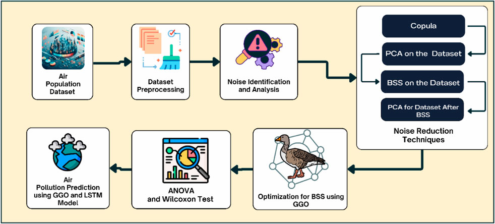
Figure 3. Proposed Framework for Air Pollution Prediction using GGO and LSTM Model.

4.1 Dataset

The dataset used in this study includes a variety of environmental and pollutant parameters collected over a period. It contains timestamps indicating the date and hour of each measurement, along with corresponding data on temperature, relative humidity, and absolute humidity. The dataset also features readings from multiple sensors that measure various environmental and pollutant levels. Additionally, it includes target values for the concentrations of key pollutants such as carbon monoxide, benzene, and nitrogen oxides. This comprehensive dataset provides a solid foundation for analyzing and predicting air pollution levels, enabling the development of effective predictive models. Key components of the dataset include:

• date_time: Timestamps indicating the specific date and hour when measurements were taken.

• deg_C: Temperature recorded in degrees Celsius.

• relative_humidity: The percentage of relative humidity in the air.

• absolute_humidity: The absolute humidity value, representing the actual amount of water vapor in the air.

• sensor_1: Measures Particulate Matter (PM), which includes particles with diameters that are generally 2.5 μm and smaller (PM_2.5).

• sensor_2: Measures Volatile Organic Compounds (VOC), which are a group of organic chemicals that can easily become vapors or gases.

• sensor_3: Measures Carbon Dioxide (CO₂), a key greenhouse gas and pollutant.

• sensor_4: Measures Ozone (O₃), a pollutant that can cause various health problems and is a component of smog.

• sensor_5: Measures Nitrogen Dioxide (NO₂), a significant air pollutant and a marker for traffic-related pollution.

• target_carbon_monoxide: The primary target variable representing the concentration of carbon monoxide (CO) in the air.

• target_benzene: The concentration of benzene (C₆H₆) in the air.

• target_nitrogen_oxides: The concentration of nitrogen oxides (NO_x) in the air.

The dataset provides detailed information on both pollutant concentrations and meteorological parameters, which are crucial for developing sophisticated models to predict air quality. The forecasting tool primarily focuses on predicting the concentration of carbon monoxide (CO), leveraging the various input features to capture the complex interactions between environmental conditions and pollutant levels.

4.2 Data preprocessing

The data preprocessing phase is discussing the core part of the proposed methodology, which aims to optimize the Air Quality Monitoring Dataset for accurate pollution forecasting. This involves multiple complicated and well-planned steps. Each adapted to deal with the specific issues and peculiarities in the given dataset. For incomplete, sporadic or sequential values, robust strategies are laid out for imputing missing observations. Emphasis is paid to sensor readings, weather information, and target variables, which could lead to a loss of accuracy in prediction if they have missing values.

Detecting and treating outliers as inliers that can be extreme values or anomalies is an integral part of the process. The uncertainty surrounding the variety of sensors’ readings and target variables could significantly throw off the predictive models. Some algorithms should require consistency in transforming variables with the same scales. This stage enhances the dataset to standardize and scale sensory readings and environmental conditions. Through these preprocessing phases, we arrive at a solid foundational position relevant to the succeeding stages (El-kenawy et al., 2022a; El-kenawy et al., 2022b).

Figure 4 Signifies a strong association of the variables in the dataset, which are displayed in the correlation matrix. The study of the correlation degree recognizes the strengthening and directional patterns. It is a guide for pointing out those variables that may have multicollinearity so that it easier to do feature selection and model building in the future.

Figure 4

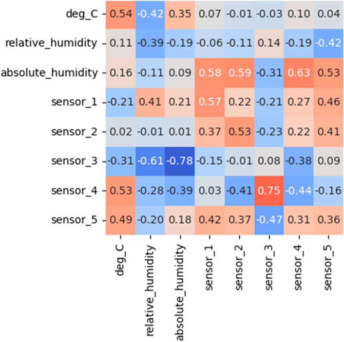
Figure 4. Correlation matrix of the dataset.

In the following stages, we expose statistics and visual representations to create a foundation for informed decision-making. Statistical parameters and graphic insights give us the necessary dictums to use the data successfully and eliminate noise more efficiently for accurate predictions.

4.3 PCA and BSS on the dataset

Our approach to accurate and reliable air pollution predictions in Section 5.3 is initiated by the PCA data applied to the original dataset, which is one of the phases of the comprehensive model. The attention now shifts to resolving noise once the Copula phase disentangled complex dependencies and correlations are reached. Such a phase is critical because it transforms the original variables into uncorrelated principal components to reduce space while retaining significant information. This part gives us a better understanding of the background, theoretical basis, steps of application, and evaluation metrics regarding PCA so that we can extend knowledge further and use this powerful tool to benefit the main goal: more accurate forecasting. Let us embark on a journey of analysis together to establish the impact of PCA on the dataset quality and also see how this stage prepares the dataset for the following stages of the noise reduction method.

PCA is a potent tool for noise reduction, capable of extracting and representing highly significant patterns within complex data. The PCA approach converts original variables into uncorrelated principal components, simplifying the dataset into its most straightforward representation. This segment delves into the reasons for choosing PCA, exploring the mathematical theory behind this technique, which effectively suppresses noise and enhances the accuracy of air pollution forecasts. PCA’s theoretical basis involves transforming the nature of the original variables into a new set of uncorrelated ones, known as principal components. These components hold the maximum information about variations, effectively filtering out noise. The mathematical principles of PCA drive essential pattern extraction and noise reduction, making it a strong contender for reducing noise in complex datasets.

BSS, a robust approach, begins its role in complex datasets by significantly enhancing the accuracy of air pollution prediction. This section delves into the theoretical foundations of BSS models and underscores their primary function as noise reduction units. It also outlines the sequential steps used in applying BSS to the dataset, providing a clear roadmap for its implementation and the evaluation metrics used to measure its impact. Understanding BSS is crucial as it forms the basis for the subsequent.

BSS is the primary problem of this paper, which is to examine and solve the different noises found in the dataset. The noise sources, like sensor errors, fluctuations, and irregular data gaps and absences, contribute to the obscuration of the actual patterns in air pollution data. Through its ability to distinguish independent sources, BSS can deliver custom paper to extract noise from genuine signals. BSS can isolate natural signals, thereby improving the quality of data, which used to develop more accurate air pollution predictions. In this regard, the BSS is expected to produce a high-quality dataset that comprises clean data, where the individual pollutant sources are classified, thus generating a new dataset with clear and precise representation. The primary effects include an increased signal-to-noise ratio, higher model interpretability, and a more refined dataset that provides a solid platform for further modeling stages.

4.4 PCA for BSS in noise reduction

The application of PCA (Principal Component Analysis) into the BSS (Blind Source Separation) process is the most important among all the other enhancements that this approach has brought, and this has been majorly demonstrated in the process of automatic transcription of music with the Air Quality Monitoring Dataset. PCA also handles issues like noise mitigation to ensure data quality and, possibly, increase the accuracy of air pollution forecasts. Theoretical underpinnings regarding PCA within the BSS framework was delineated, and steps applied to the dataset was explained (Salem and Hussein, 2019).

The application of PCA consistently as BSS gives outstanding capabilities when applied together. It can make out the primary data features in the dataset. It can also do an excellent job of reducing dimensionality, aiding signal separation and noise elimination. Orthogonalizing-based variables reduce the data into understandable amongst the complexity by retaining vital data; this, therefore, aids in the separation of independent sources in the data space. The integration of PCA within BSS offers a solution to the persistent noise problem. It facilitates better separation of independent sources, leading to a cleaner dataset for accurate air pollution prediction. The forecasted results, including a significant augmentation of signal-to-noise ratio, enhanced explanatory capabilities, and a more robust dataset for modeling, instill confidence in the effectiveness of PCA in improving data quality.

The PCA process under BSS comprises the following primary steps: preprocessing to ensure dataset quality, dimensional reduction and noise cancellation of the factorial applied by the factor-analytic method, and validation analysis to verify the statistical significance and methodological effectiveness. Evaluation metrics with insignias SDR, ISR, and SAS enable PCA performance assessment, assisting in a comparative analysis disregarding other noise models.

The effectiveness of PCA for data whitening opens avenues for further research on noise reduction in subsequent stages. The refined dataset is a crucial feature for optimization algorithms, propelling pollution prediction models to the next level with more precise and efficient performance.

4.5 BSS optimization using GGO

which concentrates on developing noise reduction techniques in air pollution prediction and provides a new hybrid method combining GGO optimization and the BSS. Greylag Goose Optimization, modeled upon the natural foraging habits of geese species Greylag, presents a specialized algorithmic paper to improve the BSS procedure. This part addresses the theoretical foundation, application procedures, and evaluation strategies utilized in GGO application towards BSS improvement in countering noise. With the help of GGO, the intended target is to make step-by-step enhancements in the accuracy of noise reduction process, which contributes to scaling up overall air pollution predictions.

Greylag Goose Optimization is an algorithm based on greylag geese’s foraging behavior. Driven by nature’s processes, geese-inspired foraging optimizes the beneficial aspects of both cooperative processes and adaptation mechanisms. Optimization technique, GGO has shown effectiveness in addressing complex problems in efficient algorithm searching algorithm path. The problem of borrowing intelligence from the greylag geese community in which collective intelligence is emulated and decentralized decision-making occurs serves as a theoretical basis for the algorithm.

The utilization of GGO in BSS optimization is meant to make source separation algorithms precise. The adaptive and collaborative nature of GGO is anticipated to be user-oriented, which can ideally facilitate the BSS process, thereby boosting the ability to determine and separate the independent sources from the whole dataset. This objective is to minimize data noise even more and thus improve the dataset to be processed further. Predicted outcomes include the possibility of better selection of sources, less interference from noise and higher quality of the given dataset. GGO-optimized BSS implementation was leading objective in accurately determining the origin of emissions, which contributes to better air pollution forecasts. The GGO optimization is successfully applied, using the technology in the process to boost the output of BSS. The power of the algorithm is deemed in its form of a collaborating search, which upgrades the process of a complete characterization of mixture components.

4.6 GGO for LSTM optimization

Greylag Goose Optimization is applied to LSTM models to optimize their hyperparameters and increase forecasts’ accuracy on air pollution rates. GGO pays homage to the foraging strategy that greylag geese use to search for food where they are less likely to be trapped in the local optimum and more likely to get the global one. The algorithm begins with generating a pool of potential solutions, known as candidate solutions. It specifies an objective, commonly the Error function, such as MSE, expected from the LSTM.

During this phase, the geese try to find the solution to the problem in the solution space. For this, they move to new positions according to their current and best-known positions. In exploitation, the geese fine-tune around the known solutions by adjusting their positions nearer to the optimum. The positions are updated by employing equations involving parameters, and an attempt is made to achieve a good balance of exploration and exploitation at the end of every round.

The fitness of every candidate solution is determined by the number of correct predictions using the LSTM model on the validation set. The fitness function is the LSTM’s error on the validation set, as shown in the equation below: The best solution is chosen according to this assessment, and the position of the geese shifts for the subsequent rounds. This continues until some stopping criteria are achieved, such as the number of iterations to be reached or the error minimum desired.

In LSTM optimization, the hyperparameters, that is, the number of layers, number of units in each layer, learning rate, batch size, and dropout rate, are set as being consistent with the solutions. The GGO algorithm modifies these hyperparameters stepwise and gradually finds the best set of hyperparameters to yield the most minor error for the prediction. The original LSTM model is improved regarding the hyperparameters, which ensure that temporal properties in the air pollution data set are better captured and, thus, better forecasts are made. Therefore, this study incorporates GGO for LSTM optimization as a robust model for enriching the prediction models in environmentally related areas.

5 Experimental results

The Results section provides a detailed explanation of the results achieved while applying different optimization algorithms in BSS to reduce noise in environmentally derived datasets. This part of the paper comprehensively appraises the optimization algorithms’ performance metrics, the statistical analyses, and the comparisons between the algorithms. The findings offered valuable insights into the capacity of these algorithms to extract essential signals with noise reduction. This enhancement can improve the overall data quality to forecast environmental variables accurately. By following a systematic analysis of the results, this section offers evaluations on the relative strengths and weaknesses of the papers to be optimized, thereby giving implications in both future papers’ development and practical methods involved in noise reduction techniques.

5.1 Copula analysis results

This chapter thoroughly considers results attained from Employing Copula as a noise reduction tool in the environmental dataset (Yang, 2020; Stork et al., 2022). The chief goal is to examine Copula for noise elimination and improve the dataset for air pollution forecast. The assessment is facilitated through a comprehensive analysis of two critical descriptive figures. This correlation matrix is illustrated in Figure 5.

Figure 5

Figure 5. Correlation matrix.

The scatter copula plot constructs further insight into how this Copula remodels the data, especially the enriched areas of clarity and the signifying signals from noise. This visual representation is significant in assessing the validity of the Copula in unmasking the actual underlying relations of the environmental variables.

We want to give a complete picture of Copula’s practical impact as a useful instrument of noise reduction in the data. The discussion not only confirm Copula’s effectiveness but also work as a basis for subsequent evaluations and comparisons with the other noise reduction methodologies to perfect the dataset for the correct predictions of air pollution status.

5.2 PCA results on the original dataset

In this context, the section is devoted to an in-depth analysis of the PCA implementation process and the results it produced on the original environmental dataset (Maier et al., 2019; Pereira et al., 2022). The main goal is to reveal PCA’s effect on smoothing the noise and further increase the dataset’s suitability for air pollution modeling.

Figure 6 presents a 3D scatter plot that visualizes the dataset after applying PCA. This plot shows data points in a reduced-dimensional space defined by the first three principal components. The primary objective of this plot is to illustrate how PCA transforms the original high-dimensional data into a more manageable form while retaining the most significant variance. In this figure, the scattered data points, which are widely dispersed, indicate noise or outliers. PCA helps in identifying these scattered points, which are less relevant for building accurate models. On the other hand, the concentrated data points form distinct clusters, representing significant patterns within the dataset. These clusters are the core information that PCA retains after dimensionality reduction. Focusing on these concentrated points improves the reliability of the subsequent models. The distinction between scattered and concentrated data highlights PCA’s effectiveness in noise reduction and pattern recognition, which are essential for creating a robust prediction model.

Figure 6

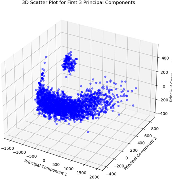
Figure 6. 3D scatter plot for first 3 principal components.

By approaching these figures, we can give a comprehensive picture of the role played by PCA in reducing the noise in the initial dataset. The discussion not only focuses on the efficacy of PCA but also prepares the reader for the second paper of the series by highlighting the follow-up evaluation, comparison with other methodologies, and the upcoming reduced noise paper for good air pollution prediction.

5.3 Original dataset’s BSS result

The importance of the BSS concept cannot be overstated in the signal processing domain, where the mixture of observations and unknown sources is being considered. This part investigates the output of different BSS approaches following the original environmental dataset, showing their excellence in noise reduction and the clearness of independent sources (Demir et al., 2020; Mushtaq and Su, 2020).

As shown in Table 2, the indicator metrics—SDR (Source-to-Distortion Ratio), ISR (Image-to-Spatial Ratio), and SAR (Source-to-Artifact Ratio)—captured the outputs from the use of BSS (Blind Source Separation) across all the variables in the dataset.

Table 2

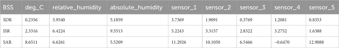
Table 2. BSS results on original dataset.

Indeed, the scatterplot in Figure 7 shows the correlation matrix depicting the linkages between the variables after the BSS. The lowering of off-diagonal elements signifies the decrease in the relationship between variables, which can indicate successful noise reduction and the separation of mixed signals.

Figure 7

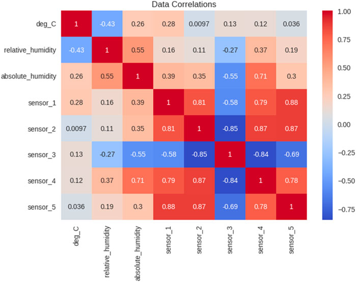
Figure 7. Correlation matrix.

Figure 8 provides a comparative visualization of the original dataset and the separated sources after applying BSS. The original data scatter plot shows mixed signals with no clear separation, indicating the presence of noise and overlapping sources. The data points in this plot are likely intermixed, making it difficult to identify distinct sources of pollution. After applying BSS, the separated sources scatter plot reveals distinct groups of data points, each representing a different source of pollution. This separation demonstrates the effectiveness of BSS in disentangling mixed signals and isolating independent sources. The clear distinction between the original and separated data underscores BSS’s capability to clean and refine the dataset, enhancing its clarity and making it more suitable for accurate air pollution prediction.

Figure 8

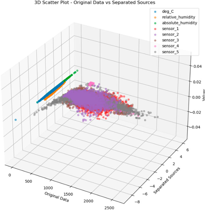
Figure 8. 3D Scatter Plot - Original Data vs. 3D Scatter Plot - Separated Sources.

To conclude, the obtained outcomes from the descriptive analysis figures reveal that BSS (Blind Source Separation) methods have a significant encouraging value. The drop in noise and the successful separation of different sources paved the way for further analyses and refinement of the data, which is essential for more accurate air pollution prediction forecasts.

5.4 Blind separated sources’ PCA

PCA is a vital technique utilized for dimensionality reduction and pattern recognition. In the BSS setting, PCA improves the dataset’s quality by extracting crucial patterns and retaining them in the data. The final paragraph highlights the PCA impact on BSS in the original dataset, including noise reduction and unmixing.

The merger of PCA and BSS is focused on combining the best possible aspects of both methodologies. BSS mainly fights with removing the signal mixture, while in PCA, the dataset is further refined by transforming it into a set of uncorrelated principal components. This section studies the consequences of PCA used in the BSS process, demonstrating the role of PCA in reducing noise and improving Source separation (Scheibler and Ono, 2020; Song et al., 2020).

In Figure 9, the original dataset’s PCA and the separated sources’ PCA results is shown. Regarding the left dependency, the scatter plot of the initial data shows that the points are scattered widely; hence, there is much noise and conflicting results. As seen on the right side of the figure, the points seem compact in the scatter plot, confirming that the BSS techniques have reduced noise and offered a suitable means of isolating the actual independent sources within the dataset.

Figure 9

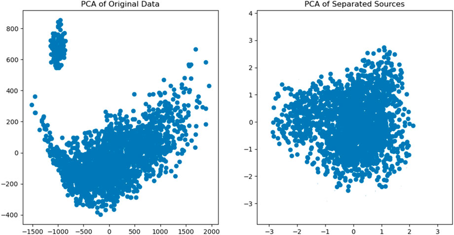
Figure 9. PCA of Original Data vs PCA of Separated Sources.

5.5 BSS optimization results

In this comprehensive comparison, we delve into the performance of BSS with various state-of-the-art optimization algorithms: Greylag Goose Optimization, Whale Optimization Algorithm (WOA), Particle Swarm Optimization (PSO), Grey Wolf Optimization (GWO) (Jinju et al., 2019; Sun et al., 2020; Zhang et al., 2020; Stergiadis et al., 2022). Table 3 shows 100 iterations each, and 10 agents for each algorithm are shown. Furthermore, those results are plotted in Table 4, Table 5, Table 6 and Table 7, as described below.

Table 3

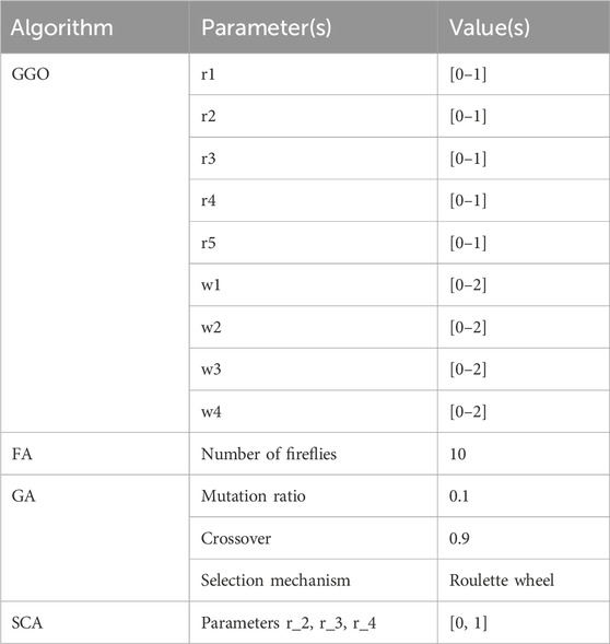
Table 3. Configuration of compared algorithms with 100 iterations and 10 agents for each one.

Table 4

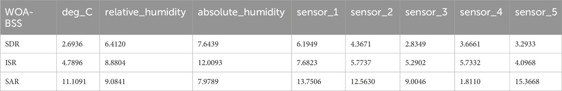
Table 4. WOA-BSS results.

Table 5

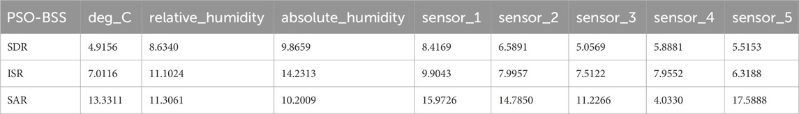
Table 5. PSO-BSS results.

Table 6

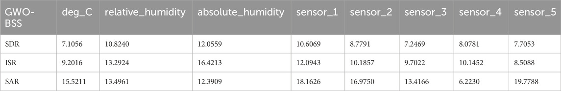
Table 6. GWO-BSS results.

Table 7

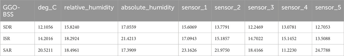
Table 7. GGO-BSS results.

As seen in Table 4, WOA-BSS results show that the polarization of the sources is an essential indicator of the performance of the Whale Optimization Algorithm. Significantly, three fundamental measures, the SDR, ISR, and SAR indices, show much higher noise reduction results for the enhanced dataset than the original (Sheeja and Sankaragomathi, 2023). For example, it inferred that the sound values of sensor 4 decreased a lot while those of sensor 5 rose sharply, showing the algorithm’s good productivity in data enhancement.

As shown in Table 5, the Particle Swarm Optimization (PSO) results are impressive and prevail for a range of sensors. The SAR values indicate this improvement for sensors 1, 4, and 5, which have different sensors to separate their sources. Furthermore, the ISR metrics demonstrate that PSO is successful at increasing the signal independence criterion, contributing significantly to the improvement of the data quality.

As shown in Table 6, GWO reflects excellent noise reduction characteristics confirmed by greater SDR, ISR, and SAR indices. GWO-BSS showcased its strength in discriminating sensors 4 and 5 for data refinement. This plays a significant role in the overall performance. The algorithm’s adaptability is demonstrated on varied datasets. It is a testimony of its efficiency in handling the noise of various complex patterns.

As shown in Table 7, the GGO Algorithm with the maximum noise reduction gets the top rank. GGO-BSS consistently scores the best SDR, ISR, and SAR values across any chosen sensor, showing its superiority in the separation task of mixed signals and improving the number of clean sources. Successfully addressing noise problems clearly expresses the asset’s robustness and efficiency. So, it is the best option when the task is to improve data quality using Blind Source Separation.

5.6 Statistical analysis for BSS optimization results

Assessing the capacity of various optimization algorithms to minimize noise by using BSS is of great importance in determining the practical utility of these algorithms. The following portion discusses the statistical analyses of tracking and evaluating the algorithm’s impact on SAR. Two main statistical methods, ANOVA (Analysis of Variance) and the Wilcoxon Signed Rank Test, are used to understand mean and median differences in SAR scores (Cai et al., 2019; Houssein et al., 2021). These analyses provide a complete explanation of the functionality of different algorithms and reveal their statistical meaning and outcomes.

As can be seen from Figure 10, variance analysis (ANOVA) was an integral part of the statistical analysis we conducted. The ANOVA results can be used to diagnose what differences in the data matter the most, leading to an evaluation of the current methodology. In this framework, the graph contrasts different elements of structure to suggest a global strategy for noise suppression and air pollution prediction.

Figure 10

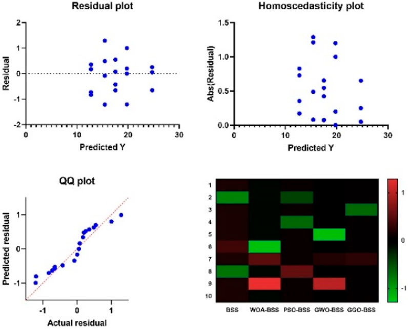
Figure 10. Analysis plots of the ANOVA test results.

The Wilcoxon Signed Rank Test shows clear differences in SAR medians between two alternative algorithms for optimizing the representation of the neuro signal. Consequently, the p-value summary states the relative differences in SAR values, which are scaled by varying methods of optimization, and consequently, whether they said differences are statistically non-significant at the level of which we usually take the meanings (α = 0.05) that are employed. Figure 11 outlines the Wilcoxon statistics, one of the main statistical techniques in statistical analysis methodology. The Wilcoxon signed-rank test provides a powerful tool to assess the consistency of the differences between pairs of data that are supposed to be the components of framework.

Figure 11

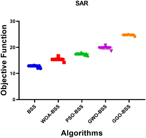
Figure 11. Sar analysis for the different optimization algorithms.

These statistical studies, however, deliver much better knowledge about the paper’s results in improving noise reduction in BSS using different optimization algorithms, which in turn contributes to more meaningful conclusions and decisions.

5.7 Air pollution prediction using GGO and LSTM model

Table 8 below compares different models, including GGO-LSTM, PSO-LSTM, GWO-LSTM, and WOA-LSTM, in predicting air pollution levels. The performance metrics include Mean Squared Error (MSE), Root Mean Squared Error (RMSE), Mean Absolute Error (MAE), Mean Bias Error (MBE), correlation coefficient (r), coefficient of determination (R²), Relative Root Mean Squared Error (RRMSE), Nash-Sutcliffe Efficiency (NSE), Willmott’s Index (WI), and the time taken to fit the model.

Table 8

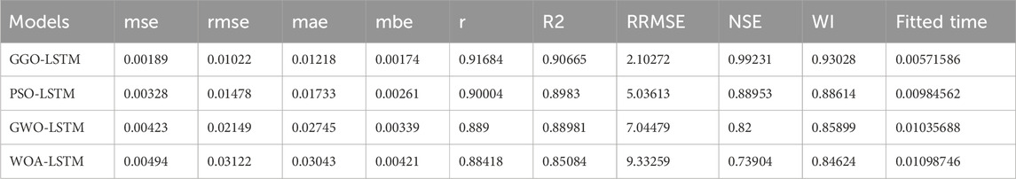
Table 8. Air Pollution Prediction using GGO and LSTM Model.

As denoted in the table, the metrics indicate that the GGO-LSTM model is the most suitable for predicting the three indexes compared to other models. It has the lowest MSE, RMSE, MAE, and MBE values, showing a higher accuracy and lesser bias when making a prediction. The correlation coefficients with values such as 0.9775 and 0.9949 are relatively higher for GGO-LSTM, which tend to have a better relationship with the predicted and actual values of cases. Further, the new development named GGO-LSTM provides the highest efficiency and model-data conformity quantified by NSE and WI. Once again, GGO-LSTM takes the least time to fit, underlining its computational advantage.

Thus, it can be mentioned that the proposed GGO-LSTM model maximally meets the requirements for effective environmental monitoring and is highly effective in terms of predicting the concentration of air pollutants.

6 Conclusion

This paper provides a methodological approach to noise control and air pollution estimation with the help of high-quality statistical and optimization apparatus. The first steps of Principal Component Analysis (PCA) eliminated noise by converting the data into principal components, whereby significant patterns were preserved while noise was removed. This step also meant that the dataset was much cleaner and easier to work with in the later steps. The Blind Source Separation (BSS) technique improved this dataset by decomposing, or in other words, disentangling signals from each other, which led to more clarity of the data. The efficiency of BSS could be clearly identified when a comparison between the original signals and the newly separated sources was made. The two were totally different since the sources of information had different points of data.

Moreover, the Copula functions used in the analysis gave a good approach to determining the dependence structure between the environmental and pollutant variables. This enabled better prediction of the relations between variables, which is vital when modeling air pollution. All in all, the Copula functions have been of great influence in the preprocessing step stage, which aims to enhance the quality of the dataset. Therefore, the Greylag Goose Optimization (GGO) algorithm was used to enhance the parameters of both PCA and BSS and the Copula functions for efficient noise elimination and source separation. Another research area involved joining GGO with LSTM networks to analyze air pollution, and the results were impressive. The GGO-LSTM scheme had the lowest MSE, RMSE, MAE, and MBE than the other optimization methods applied in the presented model.

The employment of PCA and BSS and the use of Copula functions and GGO-LSTM make the dataset clear without interference from noises, making its structures clear and easily workable for generating relatively accurate and reliable air pollution characteristics. This network-based approach is helpful for environmental surveillance. It has excellent potential when planners and policymakers use it as a tool to perform air quality management practices efficiently. This study also acknowledges the need for social research to persistently develop new noise attenuation and optimization approaches to improve predictive models in different environmental situations.

Data availability statement

The original contributions presented in the study are included in the article/Supplementary Material, further inquiries can be directed to the corresponding author.

Author contributions

AB: Writing–original draft, Writing–review and editing. AG: Writing–original draft, Writing–review and editing. IE: Writing–original draft, Writing–review and editing. EA: Writing–original draft, Writing–review and editing. ME: Writing–original draft, Writing–review and editing. E-SE-k: Writing–original draft, Writing–review and editing.

Funding

The author(s) declare financial support was received for the research, authorship, and/or publication of this article. This project was funded by the National Plan for Science, Technology and Innovation (MAARIFAH)–King Abdulaziz City for Science and Technology–the Kingdom of Saudi Arabia–award number (13-MAT377-08).

Acknowledgments

The authors thank the Science and Technology Unit, King Abdulaziz University.

Conflict of interest

The authors declare that the research was conducted in the absence of any commercial or financial relationships that could be construed as a potential conflict of interest.

Publisher’s note

All claims expressed in this article are solely those of the authors and do not necessarily represent those of their affiliated organizations, or those of the publisher, the editors and the reviewers. Any product that may be evaluated in this article, or claim that may be made by its manufacturer, is not guaranteed or endorsed by the publisher.

References

AlEisa, H., El-kenawy, E.-S., Alhussan, A., Saber, M., Abdelhamid, A., and Khafaga, D. (2022). Transfer learning for chest X-rays diagnosis using dipper Throated燗lgorithm. Comput. Mater. Continua 73 (2), 2371–2387. doi:10.32604/cmc.2022.030447

CrossRef Full Text | Google Scholar

Alharbi, A. H., Khafaga, D. S., Zaki, A. M., El-Kenawy, E.-S. M., Ibrahim, A., Abdelhamid, A. A., et al. (2024). Forecasting of energy efficiency in buildings using multilayer perceptron regressor with waterwheel plant algorithm hyperparameter. Front. Energy Res. 12. doi:10.3389/fenrg.2024.1393794

CrossRef Full Text | Google Scholar

Al-Janabi, S., Mohammad, M., and Al-Sultan, A. (2020). A new method for prediction of air pollution based on intelligent computation. Soft Comput. 24 (1), 661–680. doi:10.1007/s00500-019-04495-1

CrossRef Full Text | Google Scholar

Ansari, S., Alatrany, A. S., Alnajjar, K. A., Khater, T., Mahmoud, S., Al-Jumeily, D., et al. (2023). A survey of artificial intelligence approaches in blind source separation. Neurocomputing 561, 126895. doi:10.1016/j.neucom.2023.126895

CrossRef Full Text | Google Scholar

Arahmane, H., Hamzaoui, E.-M., Ben Maissa, Y., and Cherkaoui El Moursli, R. (2021). Neutron-gamma discrimination method based on blind source separation and machine learning. Nucl. Sci. Tech. 32 (2), 18. doi:10.1007/s41365-021-00850-w

CrossRef Full Text | Google Scholar

Asamoah, J. K. K., Owusu, M. A., Jin, Z., Oduro, F. T., Abidemi, A., and Gyasi, E. O. (2020). Global stability and cost-effectiveness analysis of COVID-19 considering the impact of the environment: using data from Ghana. Chaos, Solit. Fractals 140, 110103. doi:10.1016/j.chaos.2020.110103

CrossRef Full Text | Google Scholar

Braik, M., Sheta, A., and Al-Hiary, H. (2021). A novel meta-heuristic search algorithm for solving optimization problems: capuchin search algorithm. Neural Comput. Appl. 33 (7), 2515–2547. doi:10.1007/s00521-020-05145-6

CrossRef Full Text | Google Scholar

Cai, Z., Gu, J., Luo, J., Zhang, Q., Chen, H., Pan, Z., et al. (2019). Evolving an optimal kernel extreme learning machine by using an enhanced grey wolf optimization strategy. Expert Syst. Appl. 138, 112814. doi:10.1016/j.eswa.2019.07.031

CrossRef Full Text | Google Scholar

Chang, A., Uy, C., Xiao, X., Xiao, X., and Chen, J. (2022). Self-powered environmental monitoring via a triboelectric nanogenerator. Nano Energy 98, 107282. doi:10.1016/j.nanoen.2022.107282

CrossRef Full Text | Google Scholar

Chang, Y.-S., Chiao, H.-T., Abimannan, S., Huang, Y.-P., Tsai, Y.-T., and Lin, K.-M. (2020). An LSTM-based aggregated model for air pollution forecasting. Atmos. Pollut. Res. 11 (8), 1451–1463. doi:10.1016/j.apr.2020.05.015

CrossRef Full Text | Google Scholar

Chen, C.-H., Song, F., Hwang, F.-J., and Wu, L. (2020). A probability density function generator based on neural networks. Phys. A Stat. Mech. Its Appl. 541, 123344. doi:10.1016/j.physa.2019.123344

CrossRef Full Text | Google Scholar

Demir, F., Turkoglu, M., Aslan, M., and Sengur, A. (2020). A new pyramidal concatenated CNN approach for environmental sound classification. Appl. Acoust. 170, 107520. doi:10.1016/j.apacoust.2020.107520

CrossRef Full Text | Google Scholar

Djaafari, A., Ibrahim, A., Bailek, N., Bouchouicha, K., Hassan, M. A., Kuriqi, A., et al. (2022). Hourly predictions of direct normal irradiation using an innovative hybrid LSTM model for concentrating solar power projects in hyper-arid regions. Energy Rep. 8, 15548–15562. doi:10.1016/j.egyr.2022.10.402

CrossRef Full Text | Google Scholar

Dokeroglu, T., Sevinc, E., Kucukyilmaz, T., and Cosar, A. (2019). A survey on new generation metaheuristic algorithms. Comput. Industrial Eng. 137, 106040. doi:10.1016/j.cie.2019.106040

CrossRef Full Text | Google Scholar

El-kenawy, E.-S., Ibrahim, A., Mirjalili, S., Zhang, Y.-D., Elnazer, S., and Zaki, R. (2022b). Optimized ensemble algorithm for predicting metamaterial antenna parameters. Comput. Mater. Continua 71 (3), 4989–5003. doi:10.32604/cmc.2022.023884

CrossRef Full Text | Google Scholar

El-kenawy, E.-S. M., Zerouali, B., Bailek, N., Bouchouich, K., Hassan, M. A., Almorox, J., et al. (2022a). Improved weighted ensemble learning for predicting the daily reference evapotranspiration under the semi-arid climate conditions. Environ. Sci. Pollut. Res. 29 (54), 81279–81299. doi:10.1007/s11356-022-21410-8

CrossRef Full Text | Google Scholar

Greenacre, M., Groenen, P. J. F., Hastie, T., D’Enza, A. I., Markos, A., and Tuzhilina, E. (2022). Principal component analysis. Nat. Rev. Methods Prim. 2 (1), 100. Article 1. doi:10.1038/s43586-022-00184-w

CrossRef Full Text | Google Scholar

Halim, A. H., Ismail, I., and Das, S. (2021). Performance assessment of the metaheuristic optimization algorithms: an exhaustive review. Artif. Intell. Rev. 54 (3), 2323–2409. doi:10.1007/s10462-020-09906-6

CrossRef Full Text | Google Scholar

Hoarau, M., Angelier, F., Touzalin, F., Zgirski, T., Parenteau, C., and Legagneux, P. (2022). Corticosterone: foraging and fattening puppet master in pre-breeding greylag geese. Physiology Behav. 246, 113666. doi:10.1016/j.physbeh.2021.113666

PubMed Abstract | CrossRef Full Text | Google Scholar

Houssein, E. H., Gad, A. G., Hussain, K., and Suganthan, P. N. (2021). Major advances in particle Swarm optimization: theory, analysis, and application. Swarm Evol. Comput. 63, 100868. doi:10.1016/j.swevo.2021.100868

CrossRef Full Text | Google Scholar

Jafarzadegan, M., Safi-Esfahani, F., and Beheshti, Z. (2019). Combining hierarchical clustering approaches using the PCA method. Expert Syst. Appl. 137, 1–10. doi:10.1016/j.eswa.2019.06.064

CrossRef Full Text | Google Scholar

Jiang, H.-H., Cai, L.-M., Wen, H.-H., Hu, G.-C., Chen, L.-G., and Luo, J. (2020). An integrated approach to quantifying ecological and human health risks from different sources of soil heavy metals. Sci. Total Environ. 701, 134466. doi:10.1016/j.scitotenv.2019.134466

PubMed Abstract | CrossRef Full Text | Google Scholar

Jinju, J., Santhi, N., Ramar, K., and Sathya Bama, B. (2019). Spatial frequency discrete wavelet transform image fusion technique for remote sensing applications. Eng. Sci. Technol. Int. J. 22 (3), 715–726. doi:10.1016/j.jestch.2019.01.004

CrossRef Full Text | Google Scholar

Kahl, S., Wood, C. M., Eibl, M., and Klinck, H. (2021). BirdNET: a deep learning solution for avian diversity monitoring. Ecol. Inf. 61, 101236. doi:10.1016/j.ecoinf.2021.101236

CrossRef Full Text | Google Scholar

Khafaga, D., Alhussan, A., El-kenawy, E.-S., Ibrahim, A., H, S., El-Mashad, S., et al. (2022b). Improved prediction of metamaterial antenna bandwidth using adaptive optimization of LSTM. Comput. Mater. Continua 73 (1), 865–881. doi:10.32604/cmc.2022.028550

CrossRef Full Text | Google Scholar

Khafaga, D. S., Ibrahim, A., El-Kenawy, E.-S. M., Abdelhamid, A. A., Karim, F. K., Mirjalili, S., et al. (2022a). An Al-biruni earth radius optimization-based deep convolutional neural network for classifying monkeypox disease. Diagnostics 12 (11), 2892. Article 11. doi:10.3390/diagnostics12112892

PubMed Abstract | CrossRef Full Text | Google Scholar

Kherif, F., and Latypova, A. (2020). “Chapter 12—principal component analysis,” in Machine learning. Editors A. Mechelli, and S. Vieira (Academic Press), 209–225. doi:10.1016/B978-0-12-815739-8.00012-2

CrossRef Full Text | Google Scholar

Khosravy, M., Gupta, N., Patel, N., Dey, N., Nitta, N., and Babaguchi, N. (2020). Probabilistic Stone’s Blind Source Separation with application to channel estimation and multi-node identification in MIMO IoT green communication and multimedia systems. Comput. Commun. 157, 423–433. doi:10.1016/j.comcom.2020.04.042

CrossRef Full Text | Google Scholar

Li, X., Peng, L., Hu, Y., Shao, J., and Chi, T. (2016). Deep learning architecture for air quality predictions. Environ. Sci. Pollut. Res. 23 (22), 22408–22417. doi:10.1007/s11356-016-7812-9

CrossRef Full Text | Google Scholar

Libório, M. P., da Silva Martinuci, O., Machado, A. M. C., Machado-Coelho, T. M., Laudares, S., and Bernardes, P. (2022). Principal component analysis applied to multidimensional social indicators longitudinal studies: limitations and possibilities. GeoJournal 87 (3), 1453–1468. doi:10.1007/s10708-020-10322-0

CrossRef Full Text | Google Scholar

Ma, B., and Zhang, T. (2021). Underdetermined blind source separation based on source number estimation and improved sparse component analysis. Circuits, Syst. Signal Process. 40 (7), 3417–3436. doi:10.1007/s00034-020-01629-x

CrossRef Full Text | Google Scholar

Ma, J., Cheng, J. C. P., Lin, C., Tan, Y., and Zhang, J. (2019). Improving air quality prediction accuracy at larger temporal resolutions using deep learning and transfer learning techniques. Atmos. Environ. 214, 116885. doi:10.1016/j.atmosenv.2019.116885

CrossRef Full Text | Google Scholar

Maier, H. R., Razavi, S., Kapelan, Z., Matott, L. S., Kasprzyk, J., and Tolson, B. A. (2019). Introductory overview: optimization using evolutionary algorithms and other metaheuristics. Environ. Model. Softw. 114, 195–213. doi:10.1016/j.envsoft.2018.11.018

CrossRef Full Text | Google Scholar

Mengist, W., Soromessa, T., and Legese, G. (2020). Method for conducting systematic literature review and meta-analysis for environmental science research. MethodsX 7, 100777. doi:10.1016/j.mex.2019.100777

PubMed Abstract | CrossRef Full Text | Google Scholar

Monakhova, Y. B., and Rutledge, D. N. (2020). Independent components analysis (ICA) at the “cocktail-party” in analytical chemistry. Talanta 208, 120451. doi:10.1016/j.talanta.2019.120451

PubMed Abstract | CrossRef Full Text | Google Scholar

Mushtaq, Z., and Su, S.-F. (2020). Environmental sound classification using a regularized deep convolutional neural network with data augmentation. Appl. Acoust. 167, 107389. doi:10.1016/j.apacoust.2020.107389

CrossRef Full Text | Google Scholar

Nath, P., Saha, P., Middya, A. I., and Roy, S. (2021). Long-term time-series pollution forecast using statistical and deep learning methods. Neural Comput. Appl. 33 (19), 12551–12570. doi:10.1007/s00521-021-05901-2

PubMed Abstract | CrossRef Full Text | Google Scholar

Navares, R., and Aznarte, J. L. (2020). Predicting air quality with deep learning LSTM: towards comprehensive models. Ecol. Inf. 55, 101019. doi:10.1016/j.ecoinf.2019.101019

CrossRef Full Text | Google Scholar

Oosugi, N., Kitajo, K., Hasegawa, N., Nagasaka, Y., Okanoya, K., and Fujii, N. (2017). A new method for quantifying the performance of EEG blind source separation algorithms by referencing a simultaneously recorded ECoG signal. Neural Netw. 93, 1–6. doi:10.1016/j.neunet.2017.01.005

PubMed Abstract | CrossRef Full Text | Google Scholar

Pereira, J. L. J., Oliver, G. A., Francisco, M. B., Cunha, S. S., and Gomes, G. F. (2022). A review of multi-objective optimization: methods and algorithms in mechanical engineering problems. Archives Comput. Methods Eng. 29 (4), 2285–2308. doi:10.1007/s11831-021-09663-x

CrossRef Full Text | Google Scholar

Pion-Tonachini, L., Kreutz-Delgado, K., and Makeig, S. (2019). The ICLabel dataset of electroencephalographic (EEG) independent component (IC) features. Data Brief 25, 104101. doi:10.1016/j.dib.2019.104101

PubMed Abstract | CrossRef Full Text | Google Scholar

Ravindra, K., Rattan, P., Mor, S., and Aggarwal, A. N. (2019). Generalized additive models: building evidence of air pollution, climate change and human health. Environ. Int. 132, 104987. doi:10.1016/j.envint.2019.104987

PubMed Abstract | CrossRef Full Text | Google Scholar

Razmkhah, H., Fararouie, A., and Ravari, A. R. (2022). Multivariate flood frequency analysis using bivariate copula functions. Water Resour. Manag. 36 (2), 729–743. doi:10.1007/s11269-021-03055-3

CrossRef Full Text | Google Scholar

Rizk, F. H., Arkhstan, S., Zaki, A. M., Kandel, M. A., and Towfek, S. K. (2023). Integrated CNN and waterwheel plant algorithm for enhanced global traffic detection. J. Artif. Intell. Metaheuristics 6 (Issue 2), 36–45. doi:10.54216/JAIM.060204

CrossRef Full Text | Google Scholar

Rizk, F. H., Elshabrawy, M., Sameh, B., Mohamed, K., and Zaki, A. M. (2024). Optimizing student performance prediction using binary waterwheel plant algorithm for feature selection and machine learning. J. Artif. Intell. Metaheuristics 7 (Issue 1), 19–37. doi:10.54216/JAIM.070102

CrossRef Full Text | Google Scholar

Salem, N., and Hussein, S. (2019). Data dimensional reduction and principal components analysis. Procedia Comput. Sci. 163, 292–299. doi:10.1016/j.procs.2019.12.111

CrossRef Full Text | Google Scholar

Sawada, H., Ono, N., Kameoka, H., Kitamura, D., and Saruwatari, H. (2019). A review of blind source separation methods: two converging routes to ILRMA originating from ICA and NMF. APSIPA Trans. Signal Inf. Process. 8, e12. doi:10.1017/ATSIP.2019.5

CrossRef Full Text | Google Scholar

Scheibler, R., and Ono, N. (2020). Fast and stable blind source separation with rank-1 updates. ICASSP 2020 - 2020 IEEE Int. Conf. Acoust. Speech Signal Process. (ICASSP), 236–240. doi:10.1109/ICASSP40776.2020.9053556

CrossRef Full Text | Google Scholar

Sheeja, J. J. C., and Sankaragomathi, B. (2023). Speech dereverberation and source separation using DNN-WPE and LWPR-PCA. Neural Comput. Appl. 35 (10), 7339–7356. doi:10.1007/s00521-022-07884-0

CrossRef Full Text | Google Scholar

Song, R., Zhang, S., Cheng, J., Li, C., and Chen, X. (2020). New insights on super-high resolution for video-based heart rate estimation with a semi-blind source separation method. Comput. Biol. Med. 116, 103535. doi:10.1016/j.compbiomed.2019.103535

PubMed Abstract | CrossRef Full Text | Google Scholar

Stergiadis, C., Kostaridou, V.-D., and Klados, M. A. (2022). Which BSS method separates better the EEG Signals? A comparison of five different algorithms. Biomed. Signal Process. Control 72, 103292. doi:10.1016/j.bspc.2021.103292

CrossRef Full Text | Google Scholar

Stork, J., Eiben, A. E., and Bartz-Beielstein, T. (2022). A new taxonomy of global optimization algorithms. Nat. Comput. 21 (2), 219–242. doi:10.1007/s11047-020-09820-4

CrossRef Full Text | Google Scholar

Sun, L., Zhu, G., and Li, P. (2020). Joint constraint algorithm based on deep neural network with dual outputs for single-channel speech separation. Signal, Image Video Process. 14 (7), 1387–1395. doi:10.1007/s11760-020-01676-6

CrossRef Full Text | Google Scholar

Szipl, G., Loth, A., Wascher, C. A. F., Hemetsberger, J., Kotrschal, K., and Frigerio, D. (2019). Parental behaviour and family proximity as key to gosling survival in Greylag Geese (Anser anser). J. Ornithol. 160 (2), 473–483. doi:10.1007/s10336-019-01638-x

PubMed Abstract | CrossRef Full Text | Google Scholar

Wang, W., Fan, K., Ouyang, Q., and Yuan, Y. (2022). Acoustic UAV detection method based on blind source separation framework. Appl. Acoust. 200, 109057. doi:10.1016/j.apacoust.2022.109057

CrossRef Full Text | Google Scholar

Xiao, Q., Liu, Y., Zhou, L., Liu, Z., Jiang, Z., and Tang, L. (2022). Reliability analysis of bridge girders based on regular vine Gaussian copula model and monitored data. Structures 39, 1063–1073. doi:10.1016/j.istruc.2022.03.064

CrossRef Full Text | Google Scholar

Yang, H., Cheng, Y., and Li, G. (2021). A denoising method for ship radiated noise based on Spearman variational mode decomposition, spatial-dependence recurrence sample entropy, improved wavelet threshold denoising, and Savitzky-Golay filter. Alexandria Eng. J. 60 (3), 3379–3400. doi:10.1016/j.aej.2021.01.055

CrossRef Full Text | Google Scholar

Yang, J., Guo, Y., Yang, Z., and Xie, S. (2019). “Under-determined convolutive blind source separation combining density-based clustering and sparse reconstruction in time-frequency domain,” in IEEE Transactions on Circuits and Systems I: Regular Papers (IEEE). Available at: https://ieeexplore.ieee.org/abstract/document/8701504.

CrossRef Full Text | Google Scholar

Yang, X.-S. (2020). Nature-inspired optimization algorithms: challenges and open problems. J. Comput. Sci. 46, 101104. doi:10.1016/j.jocs.2020.101104

CrossRef Full Text | Google Scholar

Zaki, A. M., Khodadadi, N., Lim, W. H., and Towfek, S. K. (2023a). Predictive analytics and machine learning in direct marketing for anticipating bank term deposit subscriptions. Am. J. Bus. Operations Res. 11 (Issue 1), 79–88. doi:10.54216/AJBOR.110110

CrossRef Full Text | Google Scholar

Zaki, A. M., Towfek, S. K., Gee, W., Zhang, W., and Soliman, M. A. (2023b). Advancing parking space surveillance using A neural network approach with feature extraction and dipper throated optimization integration. J. Artif. Intell. Metaheuristics 6 (Issue 2), 16–25. doi:10.54216/JAIM.060202

CrossRef Full Text | Google Scholar

Zhang, L., Shi, Z., Han, J., Shi, A., and Ma, D. (2020). “FurcaNeXt: end-to-end monaural speech separation with dynamic gated dilated temporal convolutional networks,” in MultiMedia modeling. Editors Y. M. Ro, W.-H. Cheng, J. Kim, W.-T. Chu, P. Cui, J.-W. Choiet al. (Springer International Publishing), 653–665. doi:10.1007/978-3-030-37731-1_53

CrossRef Full Text | Google Scholar