Application of gene expression programing in predicting the concentration of PM2.5 and PM10 in Xi’an, China: a preliminary study

Introduction: Traditional statistical methods cannot find quantitative relationship from environmental data.

Methods: We selected gene expression programming (GEP) to study the relationship between pollutant gas and PM_2.5 (PM₁₀). They were used to construct the relationship between pollutant gas and PM_2.5 (PM₁₀) with environmental monitoring data of Xi’an, China. GEP could construct a formula to express the relationship between pollutant gas and PM_2.5 (PM₁₀), which is more explainable. Back Propagation neural networks (BPNN) was used as the baseline method. Relevant data from January 1st 2021 to April 26th 2021 were used to train and validate the performance of the models from GEP and BPNN.

Results: After the models of GEP and BPNN constructed, coefficient of determination and RMSE (Root Mean Squared Error) are used to evaluate the fitting degree and measure the effect power of pollutant gas on PM_2.5 (PM₁₀). GEP achieved RMSE of [8.7365–14.6438] for PM_2.5; RMSE of [13.2739–45.8769] for PM₁₀, and BP neural networks achieved average RMSE of [13.8741–34.7682] for PM_2.5; RMSE of [29.7327–52.8653] for PM₁₀. Additionally, experimental results show that the influence power of pollutant gas on PM_2.5 (PM₁₀) situates between −0.0704 and 0.6359 (between −0.3231 and 0.2242), and the formulas are obtained with GEP so that further analysis become possible. Then linear regression was employed to study which pollutant gas is more relevant to PM_2.5 (PM₁₀), the result demonstrates CO (SO₂, NO₂) are more related to PM_2.5 (PM₁₀).

Discussion: The formulas produced by GEP can also provide a direct relationship between pollutant gas and PM_2.5 (PM₁₀). Besides, GEP could model the trend of PM_2.5 and PM₁₀ (increase and decrease). All results show that GEP can be applied smoothly in environmental modelling.

Introduction

PM (particulate matter) has become a dangerous threat for the health of human beings (Nel, 2005; Sun et al., 2013; Apte et al., 2015; Bossmann et al., 2016). PM_2.5 or PM₁₀ are particles with a diameter less than 2.5 µm or 10 µm (Francesca Dominici et al., 2014; Pui et al., 2014) (Ostro et al., 2006; Ma et al., 2011), which have adverse health effects on respiratory health and cause more complications. The formation mechanism and process for PM_2.5 or PM₁₀ are pretty complex. Major sources of PM_2.5 and PM₁₀ include natural sources (plant division and spore, soil dust, sea salt, forest fire, volcano eruption and so on) and artificial sources (combustion of fuel, emission of industrial production process, and emission of transportation and so on); all these can be divided into disposable particles (particles that are emitted from the emission source directly) and secondary particles (particles that are released from the chemical reaction of emission and composition of the atmosphere). They mainly consist of water-soluble ions, particulate organic matter, and trace elements. Gautam et al. (2016) considers that NO₂, SO₂, CO, and O₃ are the main gaseous materials which can influence the concentrations of PM_2.5 and PM₁₀ under certain environmental conditions, so finding the association between pollutant gases and PM_2.5 (PM₁₀) is of importance.

Because of the adverse effects caused by PM_2.5 and PM₁₀ in many aspects, they are hot topics for research. Although many research studies have made plenty of achievements, the main research method is regression, time-series regression, or some existing mathematical models. In addition, the models adopted in some research studies can only produce qualitative results without direct interoperability (shown as a formula), whereas the current research adopts gene expression programing (GEP), which can effectively avoid the subjectivity of the empirical model and obtain quantitative results. We focused on modeling the relationship between PM_2.5 (PM₁₀) and pollutant gases. There are totally five types of pollutant gases, namely, SO₂, NO₂, CO, average concentration of ozone in 1 hour, and average concentration of ozone in 8 hours. We collected relevant data from Xi’an, Shaanxi province in China, which is seriously threatened by PM, and then applied GEP to complete this task. The back propagation neural network (BPNN) was used as the baseline method. Experimental results indicate that the average influence power of pollutant gases on PM_2.5 (PM₁₀) ranges from -0.0704 to 0.6359 (from -0.3231 to 0.2242), and at the same time, PM_2.5 is more seriously affected by pollutant gases than PM₁₀. Furthermore, the formulas obtained by GEP can portray the relationship and evolution law between pollutant gases and PM_2.5 (PM₁₀), and these results can be applied to predict the concentrations of PM_2.5 and PM₁₀. Furthermore, these formulas can provide more conclusions about this problem with the assistance of mathematical analysis, such as the effect of weather or season on PM_2.5 (PM₁₀), and even the above methods can be applied in this field for other perspectives. Finally, linear regression was used to study which pollutant gas more seriously influences the concentrations of PM_2.5 and PM₁₀. Experimental results show that different pollutant gases affect PM_2.5 and PM₁₀ concentrations with varying degrees, especially CO and SO₂ contribute to PM_2.5 more and NO₂ is more relevant to PM₁₀ overall. More data, including more abundant information, need to be employed to build a more generalized model that can help researchers control air pollutants and study the change of PM_2.5 (PM₁₀). Experimental results show that GEP can be used in environmental modeling to uncover essential laws hidden in environmental data.

Methods

GEP

Gene expression programing (GEP) was proposed by a Portuguese scholar, Candida, in 2001 on the basis of genetic algorithms (GA) and genetic programing (GP) (Ferreira, 2001a). GEP adopts a dual structure (genotype and phenotype), which retains the advantages of GA and GP, while at the same time avoiding their shortcomings. GEP has many advantages, such as a concise algorithm flow, as shown in Figure 1A, simple implementation, high precision, and exceptional performance in complex function finding problems with large amounts of data (Özcan, 2012; Mostafa and El-Masry, 2016). GEP uses computers to create a virtual creature population that consists of some chromosomes to simulate the genetic and evolution processes of creatures that can be carried out with a series of simulation genetic operations (e.g., cross-over, mutation, and selection as the fitness) during multi-generation iterations to guarantee that the virtual population evolves to the global optima. Cross-over, mutation, and selection simulate the reproduction, mutation, and natural selection processes. GEP has an ingenious individual encoding method, which is uncomplicated and makes subsequent genetic operations convenient to implement. It then applies the outstanding computing performance of computers to iteratively calculate and obtain an optimal function model. GEP has been fully applied in many fields, such as human body mechanics (Yang et al., 2016), water conservancy (Azamathulla, 2012) robotics (Wu et al., 2013), and agriculture (Yassin et al., 2016).

Figure 1

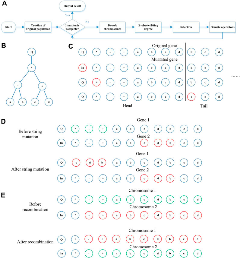
Figure 1. Details of GEP. (A) Flowchart of GEP for constructing the relationship between pollutant gases and PM_2.5 (PM₁₀). (B) The tree architecture of a gene. (C) The mutation operation: we show this operation in terms of a gene, and the green element is mutated to be the red ones. (D) String mutation: the green substring is mutated to be the red substring; here, we only show the insertion sequence transposition. (E) Recombination: the green substring and the red substring exchanged; here, we only show the single-point recombination.

As the inheritance and expansion of GA and GP, GEP integrates the advantages of both and has a more powerful ability to solve problems. The GEP algorithm can be defined as a nine-meta group: $GEP=\left\{C,E,P_0,M,\phi ,\mathrm{\Gamma },\mathrm{\Phi },\mathrm{\Pi },\mathrm{{\rm T}}\right\}$, where C is the individual’s coding means; E is the individual’s fitness evaluating function; $P_0$ is the initial population; M is the size of the population; $\phi$ is the selection operator; $\mathrm{\Gamma }$ is the crossover operator; $\mathrm{\Phi }$ is the point mutation operator; $\mathrm{\Pi }$ is the string mutation operator; and $\mathrm{{\rm T}}$ is the termination condition. In GEP, each individual is also known as a chromosome, which is formed by genes that are linked together by the link operator. The gene is a linear symbol string which is composed of a head and a tail. The head involves the variables that come from the variable set (in this problem, the variable set represents the five types of pollutant gases) and the functions that come from the function set, which can be set ahead, but the tail only contains the variables that come from the variable set. The relationship between the length of the head ($h$) and the length of the tail ($t$) is expressed as $t=h*\left(n-1\right)+1$, where $n$ is the maximum number of parameters of each function in the function set. Each individual (chromosome) in the population could be expressed as a formula (e.g., Figure 1B shows a formula $\sqrt{\left(a-b\right)*\left(c+d\right)}$), and the population could evolve according to the fitness evaluation function via genetic operations ($\mathrm{\Gamma },\mathrm{\Phi },\mathrm{\Pi }$). The genetic operations include point mutation, string mutation, and recombination. The rules of point mutation are as follows (shown in Figure 1C): the first element in the head could only be mutated to be a function in the function set, the other elements in the head could be mutated to be a function in the function set or a variable in the variable set, and the elements in the tail could only be mutated to be a variable in the variable set. The rule of string mutation is as follows: a substring in a gene is replaced by a substring in another gene within a chromosome, including insertion sequence transposition, root transposition, and gene transposition (Figure 1D). The rule of recombination is as follows: the same positions of two chromosomes are exchanged, including single-point recombination, two-point recombination, and gene combination (Figure 1E). The selection operation is roulette wheel sampling, which means the chromosome showing better fitness could be selected with a higher probability and the chromosome showing worse fitness could be selected with a lower probability. This could improve the population diversity, which is good for evolutionary computation (Ferreira, 2001b). For the problem given in this study, the result from GEP is probably a function $f\left(x_1,x_2,x_3,x_4,x_5\right)=\tan \left(x_1\right)+\left|x_2\right|+{\log }_2\left(x_3/x_5\right)+x_4/2$ which can perfectly demonstrate the relationship between the concentration of PM_2.5 (PM₁₀) and the concentrations of five types of pollutant gases (x₁, x₂, x₃, x₄, and x₅) globally.

BP neural network

The BP neural network (Liu et al., 2015), whose structure is shown in Figure 2, is a commonly used artificial network architecture. The BP neural network makes use of fully connected neurons to form a feedforward network and then adjusts the weights of each pair of connections and the biased value of each neuron with a gradient descent algorithm that is based on the chain law of derivatives.

Figure 2

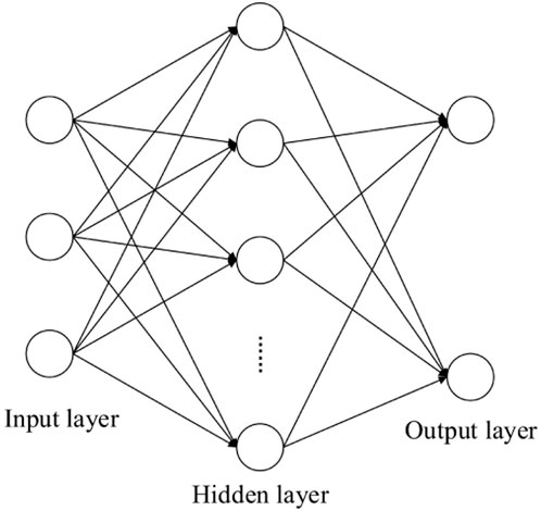
Figure 2. Architecture of the BP neural network.

Given the training dataset $\left[x_1,d_1;...x_i,d_i;...;x_n,d_n\right]$, where $x_i$ and $d_i$ are the independent variable vector and dependent variable vector, respectively. There are two procedures in the training process of the BP neural network: first, the output of the kth neuron in the output layer is shown in Eq. 1, where $w_{ij}$, $w_{jk}^{\prime }$, $b_j$, $b_k^{\prime }$, and $f\left(\cdot \right)$ are the weights between the ith input neuron and the jth hidden neuron, the weight between the jth hidden neuron and the kth output neuron, the biased value of the jth hidden neuron, the biased value of the kth output neuron, and the activation function of the hidden layer, respectively; second, the weights are adjusted according to Eq. 3, which originates from the chain rule and error function e, which is shown in Eq. 2, where ${\delta }_k=d_k-outpu{t}_k$. These two procedures are repeated until the error function converges. In this research, the input and the output of the neural network which is applied to obtain an approximate numerical regression model depicting the association between five types of pollutant gases and PM_2.5 (PM₁₀) are the concentrations of five types of pollutant gases and the concentration of PM_2.5 (PM₁₀).

$outpu{t}_k={\displaystyle \sum _k}{w}_{jk}^{\prime }f\left({\displaystyle \sum _j}{w}_{ij}\cdot x_i+b_j\right)+b_k^{\prime },(1)$

$e=\frac{1}{2}{\displaystyle \sum _{i=1}^n}{\left(d_i-outpu{t}_i\right)}^2,(2)$

$\begin{array}{l}\Delta w_{jk}^{\prime }=-\eta \frac{\partial e}{\partial w_{jk}^{\prime }}=\eta \left(d_k-outpu{t}_k\right)f^{\prime }\left(ne{t}_k\right)\\ \Delta w_{ij}=-\eta \frac{\partial e}{\partial w_{ij}}=\eta \left({\displaystyle \sum _{k=1}^L}{\delta }_k{w}_{jk}^{\prime }\right)f^{\prime }\left(ne{t}_j\right)\end{array},(3)$

where $\eta$ is the learning rate which is set in advance. Because the neural network can fit any nonlinear function with enough neurons, it has been widely applied in many fields, such as energy (Yu and Xu, 2014), safety (Wang L. et al., 2015; Wang Y. et al., 2015), and material science (Zhou et al., 2015).

Linear regression

Similar to the BP neural network, linear regression (Frank et al., 2015) is also employed to find a linear expression that portrays the relationship between independent variables and dependent variables and is expressed as Eq. 4. It adopts least squares as the objective function to minimize the error function, which is the same as the function in the BP neural network. The coefficients of each independent variable can reflect the relevance and the degree of correlation with dependent variables. As a basic data mining and intelligence information processing technique, many achievements have been made with it, such as energy (Kicsiny, 2014; Wang et al., 2016) and mechanism (Tosun et al., 2016).

$F=a_0+a_1*x_1+...+a_n*x_n,(4)$

where $x_1-x_n$ stands for the independent variables (the concentrations of CO, SO₂, NO_2, O₃ within 1 hour, and O₃ within 8 hours); F refers to dependent variables (the concentrations of PM_2.5 or PM₁₀). In the present study, n = 5 means five types of pollutant gases.

Results

Dataset

Xi’an, which is located in northwestern China, is badly affected by PM, and we chose the samples from Xi’an as the research material. Each sample consists of the concentrations of CO, SO₂, NO₂, PM_2.5, PM₁₀, and the average concentrations of O₃ (Jerrett et al., 2009) in 1 hour or 8 hours. The dataset is collected from the environmental website of Xi’an city¹ (from 1 January 2021 to 26 April 2021), where the data are obtained from 13 monitoring sites. We selected six groups of datasets collected at five monitoring sites uniformly distributed in Xi’an and an overall average dataset of the whole city. The approximate locations of five monitoring sites are shown as Figure 3. Moreover, the incomplete samples with missing value(s) are deleted to facilitate study. For each site, three-fourth entries were used to train and one-fourth entries were randomly used to validate the model. For sites 1, 2, 3, 4, 5, and the average value of the whole city, there are 96, 104, 76, 100, 88, and 116 entries, respectively. The inputs are five types of pollutant gases (CO, SO₂, average concentration of O₃ in 8 hours, NO₂, and average concentration of O₃ in 1 hour), and the output is the concentration of PM_2.5 (PM₁₀).

Figure 3

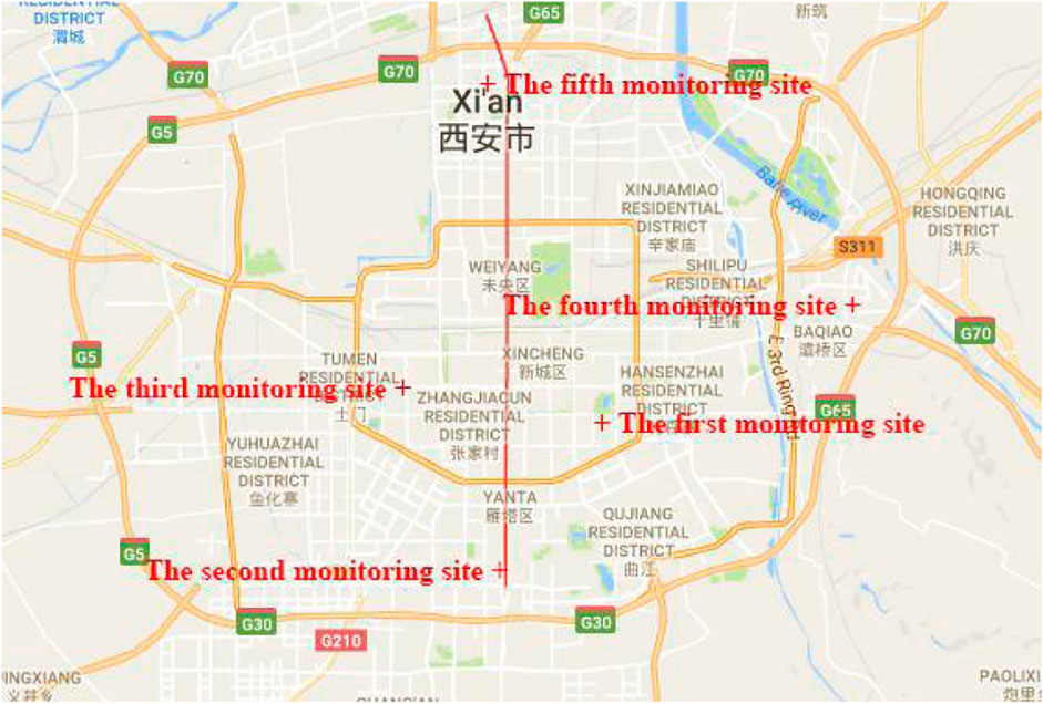
Figure 3. Probable locations of five monitoring sites.

Fitting degree evaluation function

In statistics, the coefficient of determination $1-SSE/SST$ (Kumar et al., 2020) is usually used to assess the relevance degree between two groups of data, where SSE and SST is shown as Equations 5, 6

$SSE={\displaystyle \sum _{j=1}^m}{\left(y_j-{\widehat{y}}_j\right)}^2,(5)$

$SST={\displaystyle \sum _{j=1}^m}{\left(y_j-\overline{y}\right)}^2,(6)$

where $y_j$ is the observational value of PM_2.5 (PM₁₀) and ${\widehat{y}}_j$ is the computational value, which is computed with formulas obtained with GEP (models obtained with the BP neural network) and observation values of five types of pollutant gases. $\overline{y}$ is the average value of $y$. SSE is the residual sum of squares; SST is the total sum of squares of deviations. Higher values indicate higher degrees of model fitting. On the other hand, it can be used to assess the influence power of pollutant gases on PM_2.5 and PM₁₀.

Experimental settings and experimental results

First of all, the GEP (Schmidt and Lipson, 2009) and BP neural network were used to model the influence of pollutant gases on PM_2.5 and PM₁₀. All the methods were implemented using MATLAB R2016a on a personal computer with an Intel 2.80 GHz i5 processor and 8G RAM. GEP’s initial step and genetic operations were randomly implemented as probabilities, and the weights and biased values of BP neural network were also randomly initiated. In addition, the relationship between pollutant gases and PM_2.5 (PM₁₀) is not exact. Finally, other factors contributing to PM_2.5 (PM₁₀), such as water-soluble ions, are not considered. Therefore, these two methods were repeated 10 times, and each dataset was randomly divided into two parts (three-fourth samples and one-fourth samples) for training models and validating the fitting degree of models. Because the current study aims to study the relationship between pollutant gases and PM_2.5 (PM₁₀), which is not consistent with time-series prediction, we randomly divided the datasets. Moreover, we hope to construct a more diverse dataset to observe whether GEP could model the trend of increase or decrease in PM_2.5 and PM₁₀ concentrations. The maximum, minimum, and mean values of fitting degrees are shown in Table 1 so that the rough effect power of pollutant gases can be explained clearly. Moreover, the results with the highest fitting result out of 10 repeated experiments are shown in Figures 4–7, where the computational values obtained with the trained model (the function model from GEP and the network model from the BP neural network) and the observational values are displayed in Figures 4–7 so that the fitting degree can be illustrated directly with these figures. The difference between Figures 4, 5 is obvious, namely, the performance of GEP is better than that of the BP neural networks. Moreover, GEP and BP neural networks performed similarly for both PM₁₀ and PM_2.5, indicating that pollutant gases did not contribute much more to PM₁₀ than PM_2.5 (Figure 4 versus Figures 5, 6 versus Figure 7). Similarly, BP neural networks performed no better than GEP for modeling the relationship between pollutant gases and PM₁₀. Although GEP cannot completely fit the concentration of PM_2.5 (PM₁₀) with pollutant gases, the trend of PM_2.5 (PM₁₀) can be constructed (i.e., increase or decrease). These formulas can be used to analyze the hidden laws about PM_2.5 and PM₁₀ with mathematical modeling and help predict concentrations of PM_2.5 and PM₁₀.

Table 1

Table 1. Fitting degrees of GEP and BP neural network with testing data.

Figure 4

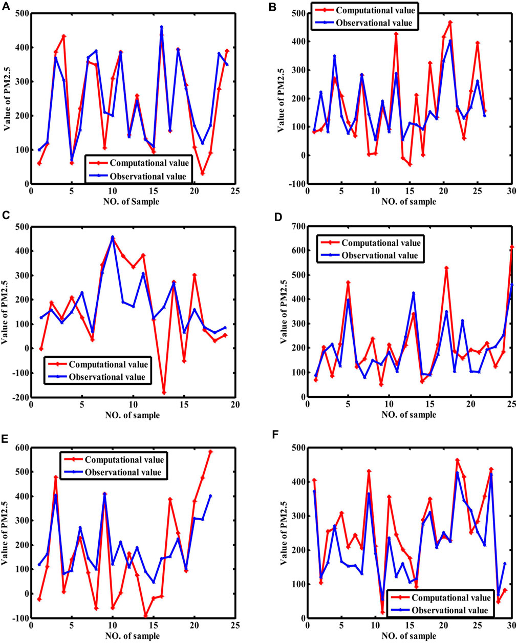
Figure 4. Fitting curves of PM_2.5 (GEP). (Note: (A–F) stand for the fitting curves obtained with datasets collected at monitoring sites 1, 2, 3, 4, 5, and average value of whole city, respectively). Because the samples are randomly selected for training and validated for repeating ten times, we only show the results with the best coefficient of determination.

Figure 5

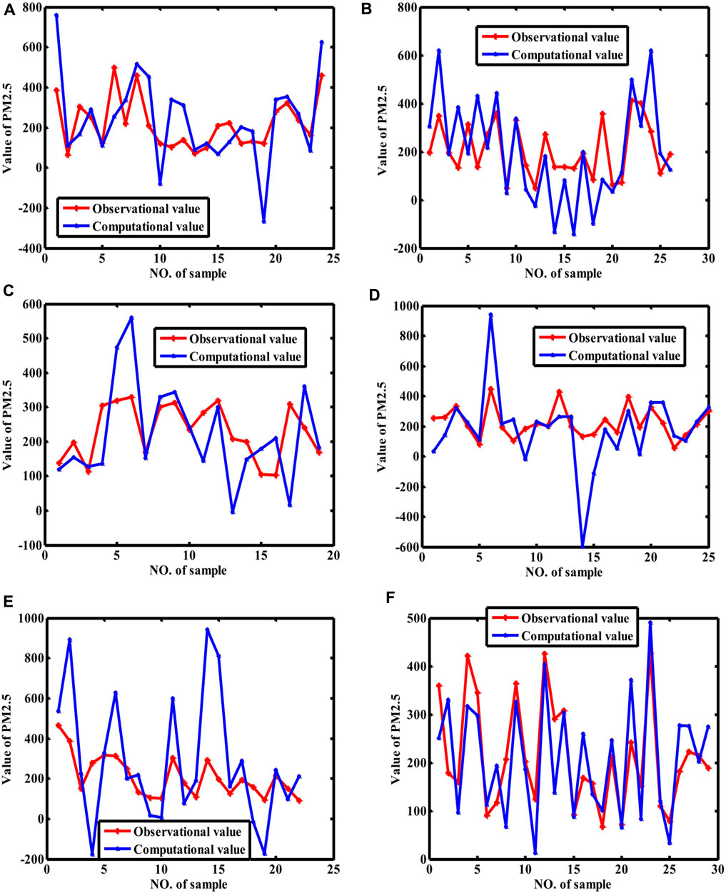
Figure 5. Fitting curves of PM_2.5 (BP neural network). [Note: (A–F) stand for the fitting curves obtained with datasets collected at monitoring sites 1, 2, 3, 4, 5, and average value of whole city, respectively]. Because the samples are randomly selected for training and validated for repeating ten times, we only show the results with the best coefficient of determination.

Figure 6

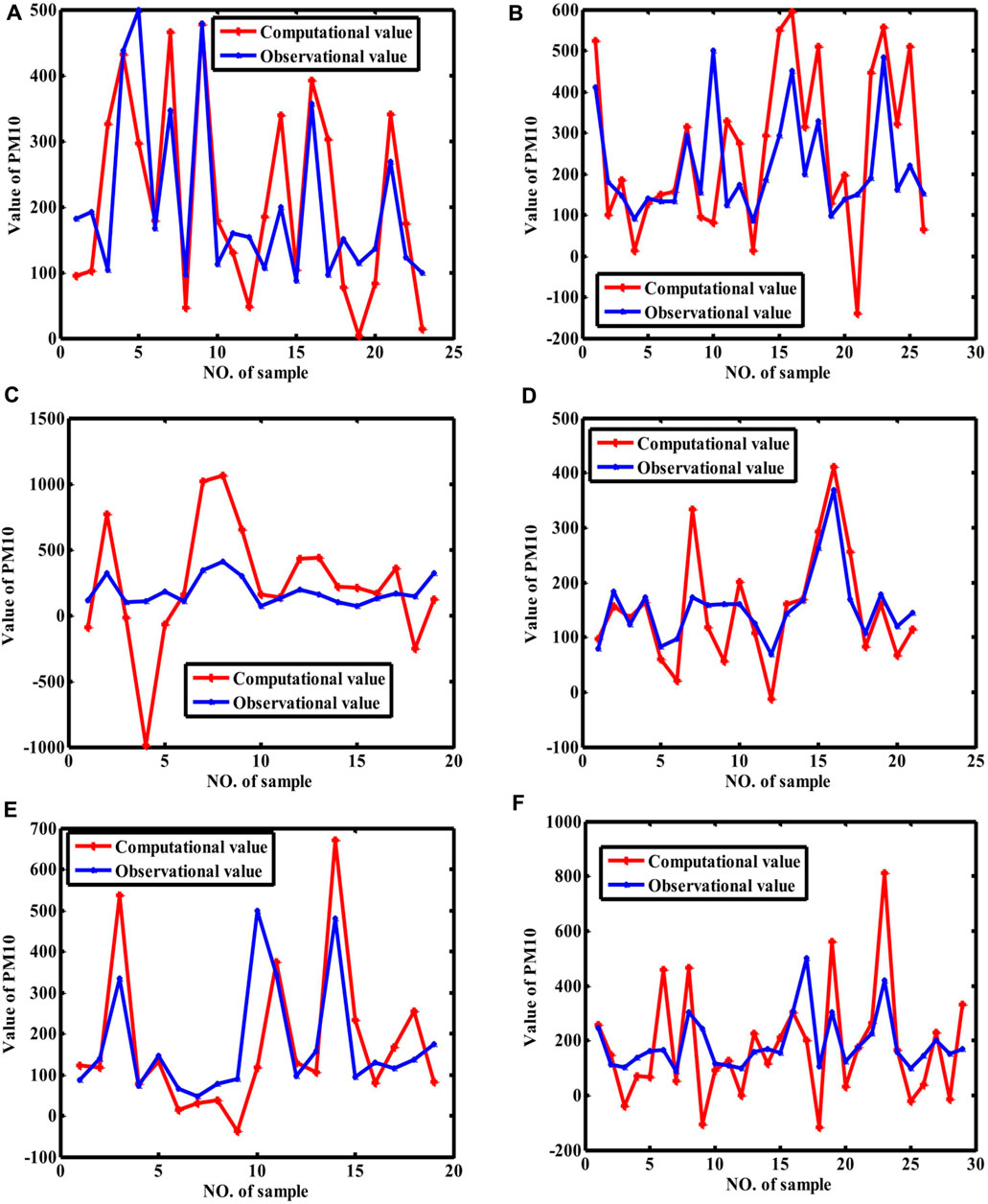
Figure 6. Fitting curves of PM₁₀ (GEP). [Note: (A–F) stand for the fitting curves obtained with datasets collected at monitoring sites 1, 2, 3, 4, 5, and average value of whole city, respectively]. Because the samples are randomly selected for training and validated for repeating ten times, we only show the result with best the coefficient of determination.

Figure 7

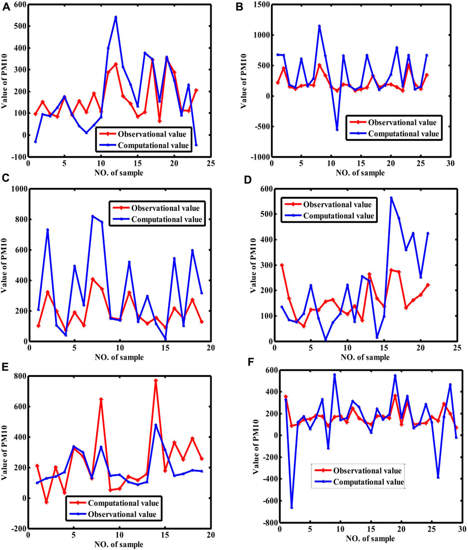
Figure 7. Fitting curves of PM₁₀ (BP neural network). [Note: (A–F) stand for the fitting curves obtained with datasets collected at monitoring sites 1, 2, 3, 4, 5, and average value of whole city, respectively]. Because the samples are randomly selected for training and validated for repeating ten times, we only show the results with the best coefficient of determination.

Discussion

Experimental results show that pollutant gases influence PM_2.5 concentrations more seriously than PM₁₀. The results from GEP show that the average influence power of pollutant gases on PM_2.5 ranges from 0.2711 to 0.6359 and the average influence power of pollutant gases on PM₁₀ ranges from -0.3231 to 0.2242. The results returned by the BP neural network indicate that the average influence power of pollutant gases on PM_2.5 ranges from −0.0704 to 0.1979 and the average influence power of pollutant gases on PM₁₀ ranges from −0.2090 to 0.1989. There are a variety of mathematical operations and formulas, such as cosine and sine functions, that could facilitate the fitting between pollutant gases and PM_2.5 (PM₁₀). At the same time, BP neural networks are easily over-fitting, and their interpretability is not better than that of GEP. The disadvantage of GEP is that it is computation-intensive; that is, the modeling process takes significantly longer than BP neural networks. The performance of GEP and BP neural networks was also evaluated by RMSE (Doreswamy et al., 2020), which is shown in Table 2. Concretely, after GEP and BPNN construct the relationship between pollutant gases and PM2.5 (PM10), the testing data could be fed into the model (GEP formula or BPNN model) to obtain the computational values of PM2.5 (PM10). Then, the computational values could be compared with observational values to figure out the coefficient of determination and RMSE. A smaller RMSE indicates better regression performance, and bigger coefficients of determination indicate better regression performance. The metrics in Table 2 also show that pollutant gases are more related with PM_2.5 than PM₁₀, and the performance of GEP is better than that of BP neural networks. In addition, the formulas with highest fitting degrees obtained by GEP are shown in Table 3.

Table 2

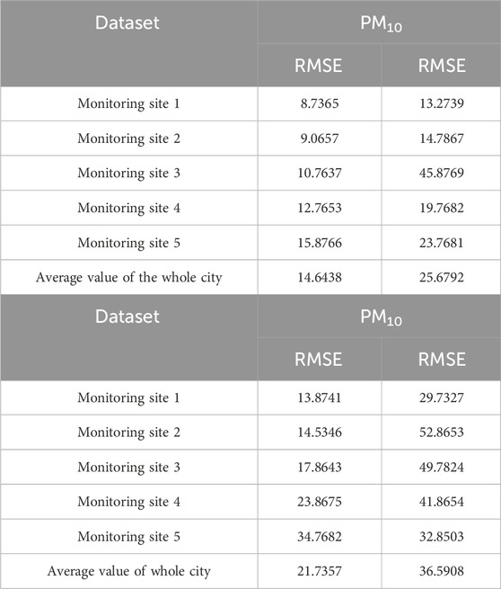
Table 2. RMSE for GEP and BP neural networks.

Table 3

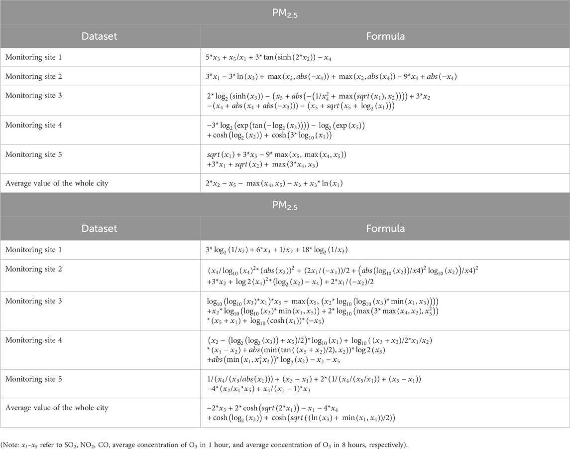
Table 3. Formulas with best fitting degrees using GEP.

Then, linear regression was applied to study which pollutant gases play more important roles than others in affecting the concentration of PM_2.5 (PM₁₀). The influence power of each type of pollutant gas on PM_2.5 (PM₁₀) can be signified by the coefficients of each item (each pollutant gas), which are shown in Table 4 in descending order. Table 4 demonstrates that the pollutant gas which is more related to PM_2.5 (PM₁₀) is different for different monitoring sites. Compared with the average concentrations of O₃ in 1 hour and 8 hours, CO and contribute to PM_2.5 more, and NO₂ and SO₂ are more relevant to PM₁₀ overall.

Table 4

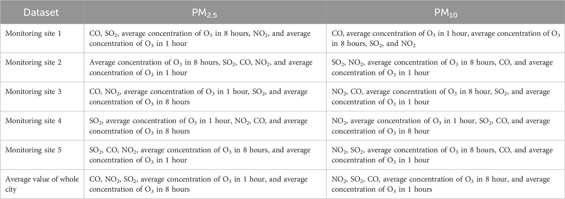
Table 4. Correlation degrees of five pollutant gases with PM_2.5 and PM₁₀.

Compared with relevant research studies on the prediction of PM_2.5 (PM₁₀) concentrations, we summarized the key information of different algorithms in Table 5. The current study did not adopt pre-processing procedures for raw data, algorithms, or evaluation metrics. The algorithms in the literature include time-series regression, which applied post-temporal PM_2.5 (PM₁₀) data to predict current PM_2.5 (PM₁₀), and regression, which applied the other factors that influence PM_2.5 (PM₁₀) to model the relationship between them. Artificial intelligence (AI) can be used to predict the concentration and the main cause of PM_2.5 (PM₁₀) to control the air quality index with the assistance of social monitoring data (vehicle, social events, meteorological factors, etc.). Moreover, the early warning for PM_2.5 (PM₁₀) could be used to improve the healthcare conditions of people. Consistent with the literature (Wang P. et al., 2015; Song et al., 2015), CO and SO₂ are the pollutant gases that are related most with PM_2.5 and PM₁₀. The main sources of CO and SO₂ are automobile exhaust and fossil fuel combustion. Therefore, we should encourage clean energy for household and industrial use. Moreover, the dataset is from 1 January to 26 April, which has cold temperatures, so the main reason for pollution is heating in the winter (the heating season in Xi’an spans from 15 November to 15 March). Because we only include the pollutant gas as an independent variable in the model, no further conclusion comes into being.

Table 5

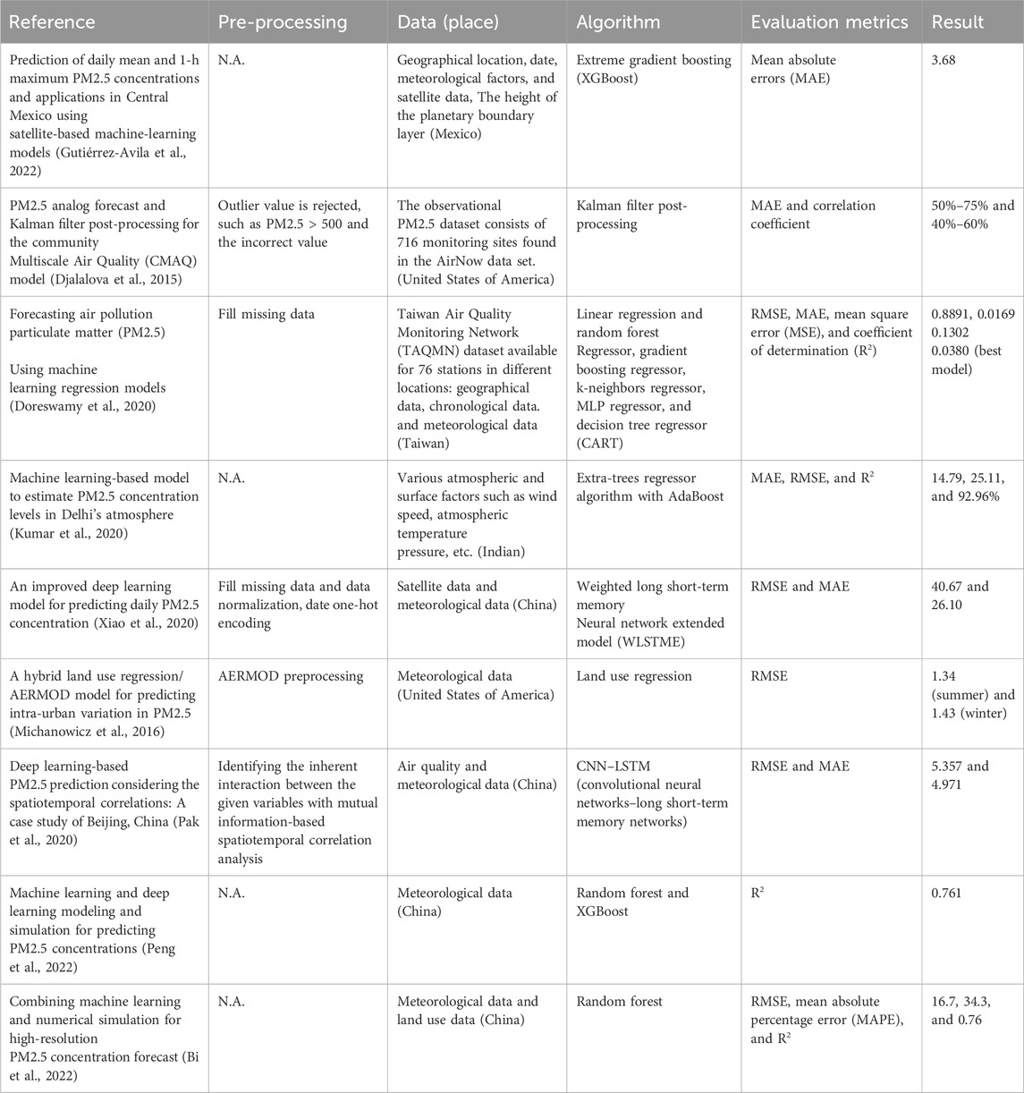
Table 5. Key points in relevant research studies.

Hypothesis and limitations

The present research only considers the effect of pollutant gases on PM_2.5 (PM₁₀); there are many other factors such as meteorological factors, human behavior, and chemical reactions that could be considered together. In addition, GEP is computation-intensive, requiring a significant amount of time. Moreover, the modeling methods should be improved, such as deep learning (Li et al., 2023), and applied to the relevant topics. Although the interpretability is improved by GEP, the formulas are not consistent with human thoughts; some novel methods could also be applied to show a more direct relationship, such as fuzzy cognitive maps (Zhang et al., 2019). Moreover, the computational resource and data resource requirement (large datasets covering more factors and more regions) impose significant burden for practice.

Conclusion

GEP was employed to model the impact of pollutant gases on concentrations of PM_2.5 (PM₁₀); the influence power is measured with the coefficient of determination. BP neural networks were used as the baseline method. Experimental results show that the influence power of pollutant gases on PM_2.5 and PM₁₀ is between -0.0704 and 0.6359 and between -0.3231 and 0.2242), respectively. The performance of the models is also compared with RMSE (root mean squared error) (Doreswamy et al., 2020). GEP achieved an RMSE of [8.7365–14.6438] for PM_2.5 and the RMSE of [13.2739–45.8769] for PM₁₀, and BP neural networks achieved the average RMSE of [13.8741–34.7682] for PM_2.5 and the RMSE of [29.7327–52.8653] for PM₁₀. For the coefficient of determination, GEP and BPNN achieved mean 0.2091–0.6539 and -0.0704–0.1979 (PM_2.5) and mean -0.3231–0.2242 and -0.1105–0.1989 (PM₁₀). GEP achieved better RMSE and coefficient of determination metrics than the BPNN. The results from GEP are more explainable than those from the BPNN because the formula could directly reflect the correlation between independent variables (pollutant gas) and dependent variables (PM_2.5/PM₁₀). The formulas obtained with GEP can be applied to study carefully to draw more conclusions from every angle. The heterogeneous relationship modeled by GEP in different seasons or specific regions could be used to monitor the causality of PM_2.5 and PM₁₀ so that pollution could be restricted. Then, results show that PM_2.5 is more correlated to CO, whereas PM₁₀ is more correlated to NO₂ and SO₂, which is inferred using linear regression. Above methods and relevant conclusions can be beneficial in controlling and forecasting PM_2.5 (PM₁₀) concentrations. Although some conclusions came into being, there are still some problems to be solved in the future, such as some negative values that will certainly not exist, which can be tackled by correcting the unreasonable chromosomes in GEP, improving the mechanism of the neural network, adjusting proper algorithm parameters for different datasets, or adding more attributes that affect PM_2.5 (PM₁₀) to the dataset. All of the above results show that GEP can be applied in environmental modeling to get more quantitative and explainable conclusions.

Data availability statement

Publicly available datasets were analyzed in this study. These data can be found here: The dataset is available: https://www.aqistudy.cn/historydata/.

Author contributions

XW: investigation, methodology, software, supervision, validation, visualization, and writing–original draft. KZ: conceptualization, formal analysis, methodology, project administration, resources, and writing–original draft. PH: project administration, resources, visualization, and writing–review and editing. MW: formal analysis, funding acquisition, visualization, and writing–review and editing. XL: data curation, investigation, methodology, and writing–review and editing. YZ: project administration, supervision, validation, and writing–review and editing. QP: investigation, methodology, validation, visualization, and writing–review and editing.

Funding

The author(s) declare that financial support was received for the research, authorship, and/or publication of this article. The Project Supported by the Natural Science Basic Research Plan in Shaanxi Province of China (2022JQ-175) and the Scientific Research Plan of Shaanxi Education Department (22JK0303).

Conflict of interest

Author KZ was employed by Chongqing Chang’an Industrial Co., Ltd. Author PH was employed by Shenzhen Metro Operation Group Co., Ltd.

The remaining authors declare that the research was conducted in the absence of any commercial or financial relationships that could be construed as a potential conflict of interest.

Publisher’s note

All claims expressed in this article are solely those of the authors and do not necessarily represent those of their affiliated organizations, or those of the publisher, the editors, and the reviewers. Any product that may be evaluated in this article, or claim that may be made by its manufacturer, is not guaranteed or endorsed by the publisher.

Footnotes

¹https://aqicn.org/city/china/xian/wentiju/cn/

References

Apte, J. S., Marshall, J. D., Cohen, A. J., and Brauer, M. (2015). Addressing global mortality from ambient PM2.5. Environ. Sci. Technol. 49, 8057–8066. doi:10.1021/acs.est.5b01236

PubMed Abstract | CrossRef Full Text | Google Scholar

Azamathulla, H. M. (2012). Gene-expression programming to predict scour at a bridge abutment. J. Hydroinformatics 14, 324–331. doi:10.2166/hydro.2011.135

CrossRef Full Text | Google Scholar

Bi, J., Knowland, K. E., Keller, C. A., and Liu, Y. (2022). Combining machine learning and numerical simulation for high-resolution PM2.5 concentration forecast. Environ. Sci. Technol. 56, 1544–1556. doi:10.1021/acs.est.1c05578

PubMed Abstract | CrossRef Full Text | Google Scholar

Bossmann, K., Bach, S., Höflich, C., Valtanen, K., Heinze, R., Neumann, A., et al. (2016). Holi colours contain PM10 and can induce pro-inflammatory responses. J. Occup. Med. Toxicol. 11, 42. doi:10.1186/s12995-016-0130-9

PubMed Abstract | CrossRef Full Text | Google Scholar

Djalalova, I., Delle Monache, L., and Wilczak, J. (2015). PM2.5 analog forecast and Kalman filter post-processing for the community multiscale air quality (CMAQ) model. Atmos. Environ. 108, 76–87. doi:10.1016/j.atmosenv.2015.02.021

CrossRef Full Text | Google Scholar

Doreswamy, K. S. H., Km, Y., and Gad, I. (2020). Forecasting air pollution particulate matter (PM2.5) using machine learning regression models. Procedia Comput. Sci. 171, 2057–2066. doi:10.1016/j.procs.2020.04.221

CrossRef Full Text | Google Scholar

Ferreira, C. (2001a). Gene expression programming: a new adaptive algorithm for solving problems. Comput. Sci., 87–129. doi:10.48550/arXiv.cs/0102027

CrossRef Full Text | Google Scholar

Ferreira, C. (2001b). Gene expression programming: a new adaptive algorithm for solving problems. arXiv preprint cs/0102027.

Google Scholar

Francesca Dominici, M. G., Sunstein, C. R., and Sunstein, C. R. (2014). Particulate matter matters. Science 344, 257–259. doi:10.1126/science.1247348

PubMed Abstract | CrossRef Full Text | Google Scholar

Frank, A., Fabregat-Traver, D., and Bientinesi, P. (2015). Large-scale linear regression: development of high-performance routines. Appl. Math. Comput. 275, 411–421. doi:10.1016/j.amc.2015.11.078

CrossRef Full Text | Google Scholar

Gautam, S., Yadav, A., Tsai, C. J., and Kumar, P. (2016). A review on recent progress in observations, sources, classification and regulations of PM 2.5 in Asian environments. Environ. Sci. Pollut. Res. Int. 23, 21165–21175. In Press. doi:10.1007/s11356-016-7515-2

PubMed Abstract | CrossRef Full Text | Google Scholar

Gutiérrez-Avila, I., Arfer, K. B., Carrión, D., Rush, J., Kloog, I., Naeger, A. R., et al. (2022). Prediction of daily mean and one-hour maximum PM2.5 concentrations and applications in Central Mexico using satellite-based machine-learning models. J. Expo. Sci. Environ. Epidemiol. 32, 917–925. doi:10.1038/s41370-022-00471-4

PubMed Abstract | CrossRef Full Text | Google Scholar

Jerrett, M., Ito, K., Thurston, G., Krewski, D., Shi, Y., Calle, E., et al. (2009). Long-term ozone exposure and mortality. N. Engl. J. Med. 360, 1085–1095. doi:10.1056/nejmoa0803894

PubMed Abstract | CrossRef Full Text | Google Scholar

Kicsiny, R. (2014). Multiple linear regression based model for solar collectors. Sol. Energy 110, 496–506. doi:10.1016/j.solener.2014.10.003

CrossRef Full Text | Google Scholar

Kumar, S., Mishra, S., and Singh, S. K. (2020). A machine learning-based model to estimate PM2.5 concentration levels in Delhi's atmosphere. Heliyon 6, e05618. doi:10.1016/j.heliyon.2020.e05618

PubMed Abstract | CrossRef Full Text | Google Scholar

Li, J., Crooks, J., Murdock, J., de Souza, P., Hohsfield, K., Obermann, B., et al. (2023). A nested machine learning approach to short-term PM2.5 prediction in metropolitan areas using PM2.5 data from different sensor networks. Sci. Total Environ. 873, 162336. doi:10.1016/j.scitotenv.2023.162336

PubMed Abstract | CrossRef Full Text | Google Scholar

Liu, S., Hou, Z., and Yin, C. (2015). Data-driven modeling for UGI gasification processes via an enhanced genetic BP neural network with link switches. IEEE Trans. Neural Netw. Learn. Syst.

Google Scholar

Ma, Y., Chen, R., Pan, G., Xu, X., Song, W., Chen, B., et al. (2011). Fine particulate air pollution and daily mortality in Shenyang, China. Sci. Total Environ. 409, 2473–2477. doi:10.1016/j.scitotenv.2011.03.017

PubMed Abstract | CrossRef Full Text | Google Scholar

Michanowicz, D. R., Shmool, J. L. C., Tunno, B. J., Tripathy, S., Gillooly, S., Kinnee, E., et al. (2016). A hybrid land use regression/AERMOD model for predicting intra-urban variation in PM2.5. Atmos. Environ. 131, 307–315. doi:10.1016/j.atmosenv.2016.01.045

CrossRef Full Text | Google Scholar

Mostafa, M. M., and El-Masry, A. A. (2016). Oil price forecasting using gene expression programming and artificial neural networks. Econ. Model. 54, 40–53. doi:10.1016/j.econmod.2015.12.014

CrossRef Full Text | Google Scholar

Nel, A. (2005). Air pollution-related illness: effects of particles. Science 308, 804–806. doi:10.1126/science.1108752

PubMed Abstract | CrossRef Full Text | Google Scholar

Ostro, B., Broadwin, R., Green, S., Feng, W. Y., and Lipsett, M. (2006). Fine particulate air pollution and mortality in nine California counties: results from CALFINE. Env. Health Perspect. 114 (1), 29–33. doi:10.1289/ehp.8335

CrossRef Full Text | Google Scholar

Özcan, F. (2012). Gene expression programming based formulations for splitting tensile strength of concrete. Constr. Build. Mater. 26, 404–410. doi:10.1016/j.conbuildmat.2011.06.039

CrossRef Full Text | Google Scholar

Pak, U., Ma, J., Ryu, U., Ryom, K., Juhyok, U., Pak, K., et al. (2020). Deep learning-based PM2.5 prediction considering the spatiotemporal correlations: a case study of Beijing, China. Sci. Total Environ. 699, 133561. doi:10.1016/j.scitotenv.2019.07.367

PubMed Abstract | CrossRef Full Text | Google Scholar

Peng, J., Han, H., Yi, Y., Huang, H., and Xie, L. (2022). Machine learning and deep learning modeling and simulation for predicting PM2.5 concentrations. Chemosphere 308, 136353. doi:10.1016/j.chemosphere.2022.136353

PubMed Abstract | CrossRef Full Text | Google Scholar

Pui, D. Y. H., Chen, S. C., and Zuo, Z. (2014). PM 2.5 in China: measurements, sources, visibility and health effects, and mitigation. Particuology 13, 1–26. doi:10.1016/j.partic.2013.11.001

CrossRef Full Text | Google Scholar

Schmidt, M., and Lipson, H. (2009). Distilling free-form natural laws from experimental data. Science 324, 81–85. doi:10.1126/science.1165893

PubMed Abstract | CrossRef Full Text | Google Scholar

Song, Y.-Z., Yang, H.-L., Peng, J.-H., Song, Y.-R., Sun, Q., and Li, Y. (2015). Estimating PM2. 5 concentrations in Xi'an city using a generalized additive model with multi-source monitoring data. PloS one 10, e0142149. doi:10.1371/journal.pone.0142149

PubMed Abstract | CrossRef Full Text | Google Scholar

Sun, Z., An, X., Tao, Y., and Hou, Q. (2013). Assessment of population exposure to PM10 for respiratory disease in Lanzhou (China) and its health-related economic costs based on GIS. BMC Public Health 13, 891. doi:10.1186/1471-2458-13-891

PubMed Abstract | CrossRef Full Text | Google Scholar

Tosun, E., Aydin, K., and Bilgili, M. (2016). Comparison of linear regression and artificial neural network model of a diesel engine fueled with biodiesel-alcohol mixtures. Alexandria Engineering Journal 55, 3081–3089. doi:10.1016/j.aej.2016.08.011

CrossRef Full Text | Google Scholar

Wang, G., Su, Y., and Shu, L. (2016). One-day-ahead daily power forecasting of photovoltaic systems based on partial functional linear regression models. Renew. Energy 96, 469–478. doi:10.1016/j.renene.2016.04.089

CrossRef Full Text | Google Scholar

Wang, L., Ren, T., Nie, B., Chen, Y., Lv, C., Tang, H., et al. (2015a). Development of a spontaneous combustion TARPs system based on BP neural network. Int. J. Min. Sci. Technol. 25, 803–810. doi:10.1016/j.ijmst.2015.07.016

CrossRef Full Text | Google Scholar

Wang, P., Cao, J., Tie, X., Wang, G., Li, G., Hu, T., et al. (2015b). Impact of meteorological parameters and gaseous pollutants on PM2. 5 and PM10 mass concentrations during 2010 in Xi’an, China. Aerosol Air Qual. Res. 15, 1844–1854. doi:10.4209/aaqr.2015.05.0380

CrossRef Full Text | Google Scholar

Wang, Y., Lu, C., and Zuo, C. (2015c). Coal mine safety production forewarning based on improved BP neural network. Int. J. Min. Sci. Technol. 25, 319–324. doi:10.1016/j.ijmst.2015.02.023

CrossRef Full Text | Google Scholar

Wu, C. H., Lin, I. S., Wei, M. L., and Cheng, T. Y. (2013). Target position estimation by genetic expression programming for mobile robots with vision sensors. IEEE Trans. Instrum. Meas. 62, 3218–3230. doi:10.1109/tim.2013.2272173

CrossRef Full Text | Google Scholar

Xiao, F., Yang, M., Fan, H., Fan, G., and Al-qaness, M. A. A. (2020). An improved deep learning model for predicting daily PM2.5 concentration. Sci. Rep. 10, 20988. doi:10.1038/s41598-020-77757-w

PubMed Abstract | CrossRef Full Text | Google Scholar

Yang, Z., Chen, Y., Tang, Z., and Wang, J. (2016). Surface EMG based handgrip force predictions using gene expression programming. Neurocomputing 207, 568–579. doi:10.1016/j.neucom.2016.05.038

CrossRef Full Text | Google Scholar

Yassin, M. A., Alazba, A. A., and Mattar, M. A. (2016). A new predictive model for furrow irrigation infiltration using gene expression programming. Comput. Electron. Agric. 122, 168–175. doi:10.1016/j.compag.2016.01.035

CrossRef Full Text | Google Scholar

Yu, F., and Xu, X. (2014). A short-term load forecasting model of natural gas based on optimized genetic algorithm and improved BP neural network. Appl. Energy 134, 102–113. doi:10.1016/j.apenergy.2014.07.104

CrossRef Full Text | Google Scholar

Zhang, K., Pan, Q., Yu, D., Wang, L., Liu, Z., Li, X., et al. (2019). Systemically modeling the relationship between climate change and wheat aphid abundance. Sci. Total Environ. 674, 392–400. doi:10.1016/j.scitotenv.2019.04.143

PubMed Abstract | CrossRef Full Text | Google Scholar

Zhou, J., Wan, X., Zhang, J., Yan, Z., and Li, Y. (2015). Modeling of constitutive relationship of aluminum alloy based on BP neural network model. Mater. Today Proc. 2, 5023–5028. doi:10.1016/j.matpr.2015.10.092

CrossRef Full Text | Google Scholar