
94% of researchers rate our articles as excellent or good
Learn more about the work of our research integrity team to safeguard the quality of each article we publish.
Find out more
ORIGINAL RESEARCH article
Front. Environ. Sci., 26 July 2024
Sec. Environmental Informatics and Remote Sensing
Volume 12 - 2024 | https://doi.org/10.3389/fenvs.2024.1416597
This article is part of the Research TopicRemote Sensing of the CryosphereView all 10 articles
 Alexander Kokhanovsky1*Maximilian Brell1Karl Segl1
 Dmitry Efremenko2Boyan Petkov3,4Giovanni Bianchini5Robert Stone6*Sabine Chabrillat1,7*
The two-LAyered snow Radiative Transfer (LART) model has been proposed for snow remote sensing applications. It is based on analytical approximations of the radiative transfer theory. The geometrical optics approximation has been used to derive the local snow optical parameters, such as the probability of photon absorption by ice grains and the average cosine of single light scattering in a given direction in a snowpack. The application of the model to the selected area in Antarctica has shown that the technique is capable of retrieving the snow grain size both in the upper and lower snow layers, with grains larger in the lower snow layer as one might expect due to the metamorphism processes. Such a conclusion is confirmed by ground measurements of the vertical snow grain size variability in Antarctica.
It has been shown in the past that multispectral measurements can be used to retrieve the vertical variation of cloud and snow properties (Li et al., 2011; Kokhanovsky and Rozanov, 2012). In this paper, we propose a fast and robust technique for the determination of the vertical variation of ice grain size in snow using hyperspectral satellite measurements, which opens the way for the large-scale assessment of the vertical inhomogeneity of various snow surfaces. The first retrievals of snow vertical inhomogeneity using EnMAP hyperspectral measurements of top-of-atmosphere (TOA) radiance are performed. EnMAP (Guanter et al., 2015; Storch et al., 2023) is the satellite mission for the assessment of various environmental parameters based on hyperspectral reflected solar light measurements in the spectral range of 410–2,450 nm with a spatial resolution of 30 m. The solution to the inverse radiative transfer problem is based on the two-LAyered snow Radiative Transfer (LART) model developed by us for the simulation of both bottom-of-atmosphere (BOA) and top-of-atmosphere spectral reflectance for the cases of underlying snow surfaces. The unique feature of this model is that it makes it possible to model the snow reflectance using simple analytical relationships between the snow nadir reflectance and ice grain sizes, which facilitates the solution of the inverse problem. Only case 1 snow is considered (dry and clean snow). However, the model can be easily generalized to the case of polluted snow. Other limitations of the forward model used in the retrieval of snow properties are listed as follows:
- the semi-infinite snow layer with no contribution from the underlying surface (1);
- the plane-parallel snow layer (the absence of 3D effects, sastrugi, surface inclination, and horizontal variability of snow properties) (2);
- the close-packed effects are ignored (3);
- the shape of particles is assumed ahead of retrievals (Koch fractals of the second generation) (4);
- only two snow layers are assumed, with the smaller ice grains at the top (5);
- the size distribution of ice crystals is not accounted for (6);
- the atmospheric aerosol optical thickness is small (7);
- the clear sky atmosphere without cloudy media and fogs between the instrument and snow surface under observation is assumed (8).
Some of the assumptions given above are not critical for the proposed theory (e.g., 1, 5, and 6) and can be removed if needed.
The remainder of this paper is structured as follows: in Section 2, we introduce the radiative transfer forward model and discuss the dependence of local and global snow characteristics on the snow microstructure and the optical thickness of the upper snow layer. In Section 3, we propose a semi-analytical approach for the inverse problem solution. In Section 4, we discuss the application of the developed technique for snow remote sensing using the EnMAP L1C radiance data.
In this work, we shall use the shortwave infrared (SWIR) EnMAP channels, where ice absorbs incoming solar radiation and atmospheric contribution (outside gaseous absorption bands) can be neglected for a clean Antarctic atmosphere. Therefore, we assume that the top-of-atmosphere reflectance in the selected channels coincides with the snow reflectance. It is supposed that the snow is composed of a semi-infinite layer underneath and a relatively thin layer of fresh snow at the top. Therefore, the snow reflectance at the cosine of the solar zenith angle
where
The value of
where a = 0.139, b = 1.17, and
is the similarity parameter,
where
where
where
where
It follows that
where
One can see that the equations given above make it possible to reduce the calculation of the reflectance of a two-layered snow to the calculation of the reflection function of a semi-infinite snow layer
This simple equation has been derived by Kokhanovsky et al. (2024) under the assumption that
The proposed LART forward model (Eqs 1–10, (Yanovitskij, 1997)) can be used to simulate the spectral nadir reflectance of snow layers. It is import to compare the results of calculations using the proposed simple analytical forward model and the numerical solution of the integro-differential radiative transfer equation (RTE) (Sobolev, 1975; Liou, 2002) for solar light reflectance. The numerical solution of the RTE was found using the PYDOME forward radiative transfer model, a Python implementation of the discrete ordinate method with a matrix exponential (DOM-ME) approach. One expands the RTE into a cosine Fourier series and transforms the light radiance in the angular domain into its discrete counterpart by selecting a discrete set of Gaussian points and weights in the framework of the DOM-ME approach. Therefore, the integral term of the RTE is changed to a simple summation operation, leading to a system of differential equations solvable via the matrix exponential method. To enhance the efficiency of solving the eigenvalue problem, a scaling transformation, as described by Efremenko et al. (2013), is applied. The theoretical foundation of this method is detailed by Efremenko et al. (2017). PYDOME operates in two modes. In the first mode, layer equations for each atmospheric layer are derived and integrated into the system. By applying boundary conditions at the top and bottom of the atmosphere and ensuring radiance continuity at layer boundaries, the system yields the unknown radiance components. In the second mode, the problem is approached through the Riccati matrix equation to determine reflection and transmission matrices (Chuprov et al., 2022). The solution for the multilayered medium is obtained using the matrix operator method, which computes the reflection and transmission matrices for the entire medium. The model incorporates several phase function truncation techniques, including the delta-M (Wiscombe, 1977) and delta-fit (Hu et al., 2000) methods and TMS (Nakajima and Tanaka, 1988) correction. An optional modification for the small-angle approximation of the discrete ordinate method is available to bypass phase function truncation (Afanas’ev et al., 2020). For this study, the first mode was utilized, augmented with delta-M and TMS correction methods. The number of discrete ordinates was increased in powers of 2 until the results from two consecutive iterations differed by less than 0.0001%. A total of 64 discrete ordinates were utilized. The necessary number of azimuthal harmonics was determined based on the Cauchy convergence criterion, which had to be satisfied twice to ensure the accuracy and reliability of the computational results. The dependence of reflectance on the upper layer optical thickness for various values of the SSA in both layers is shown in Figures 1A, B. The calculations have been performed using both the LART forward model and the numerical PYDOME RTE solution. Except for the case of SSA equal to 0.9999, the semi-infinite snow limit is achieved at the upper snow optical thickness in the range of 10–40, depending on the level of light absorption in the upper layer. The cases with a single scattering albedo larger than 0.9999 occur in the visible range (Kokhanovsky, 2021); the spectral range not used in the inverse problem solution is discussed below. Figure 1C shows that the accuracy of our forward model is excellent. The relative errors are smaller than 5% at solar zenith angles larger than 78.5°, which is comparable to the accuracy of the EnMAP measurements. This is of great importance for the simplification of both forward and inverse radiative transfer problems in layered snow optics.
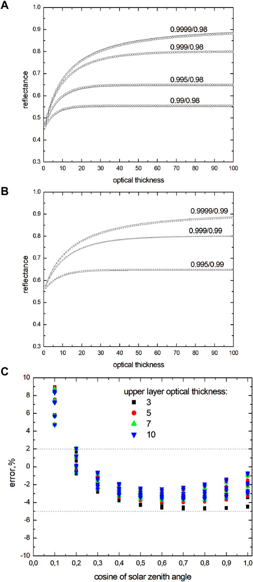
Figure 1. (A) Dependence of the reflectance of a two-layered snow system on the optical thickness of the upper layer calculated using the approximation given by Eq. 1 and the numerical solution of the radiative transfer equation for the nadir observation and the solar zenith angle 60°. It is assumed that the lower layer is semi-infinite. The phase function is the same in both layers (Henyey–Greenstein phase function with the average cosine of the scattering angle equal to 0.75). The single scattering albedo values in the upper (first number) and lower (second number) snow layers are given in the figure for each curve. (B) The same as in (A), except for the single scattering albedo of the lower layer, which is equal to 0.99. (C) The dependence of the error of the approximation given by Eq. 1 on the cosine of the solar zenith angle at the nadir observation for the several values of the upper layer optical thickness. All other parameters are the same as in (A). The spread along the vertical is due to seven combinations of the single scattering albedo values for the upper and lower layers given in (A).
To model the snow spectral reflectance using the formulas given above, one needs to calculate the values of the probability of photon absorption β, the average cosine of scattering angle g, and the extinction coefficient
where
One can see that the parameters
which strongly depends on the shape of particles and, therefore, on the type of snow. The parameters
as
The pair (σ,ε) depends on the shape of the ice grains. In this work, we shall assume that σ = 0.8571 and ε = 0.9045 as for fractal ice grains (Kokhanovsky et al., 2024).
The parameterizations for the values of
The value of
which is valid for fractal ice grains.
Eqs 13, 14 are valid for arbitrary identical nonspherical randomly oriented particles, which are much larger than the wavelength of incident light (
It should be pointed out that the extinction coefficient
where
where
where
where L is the geometrical thickness of the layer. One can see that optical thickness approximately coincides with the number of ice grain layers on the snow thickness L. In addition, the snow optical thickness can be used to estimate the upper layer snow geometrical thickness; that is, from Eq. 24:
The results of calculations of the local optical properties and also the attenuation parameter c and spherical albedo of a semi-infinite snow layer are given in Figure 2. One can see that the respective parameters vary considerably depending on the size of the particles. The same is true for the spherical albedo. This points out the fact that the determination of ice grain size is possible from optical measurements if the remote sensing channels are chosen in such a way that they provide maximal sensitivity to the snow ice grain size. Usually, one uses wavelengths 1,026 and 1,235 nm (Kokhanovsky, 2021) for the respective retrievals (see Figure 2F).
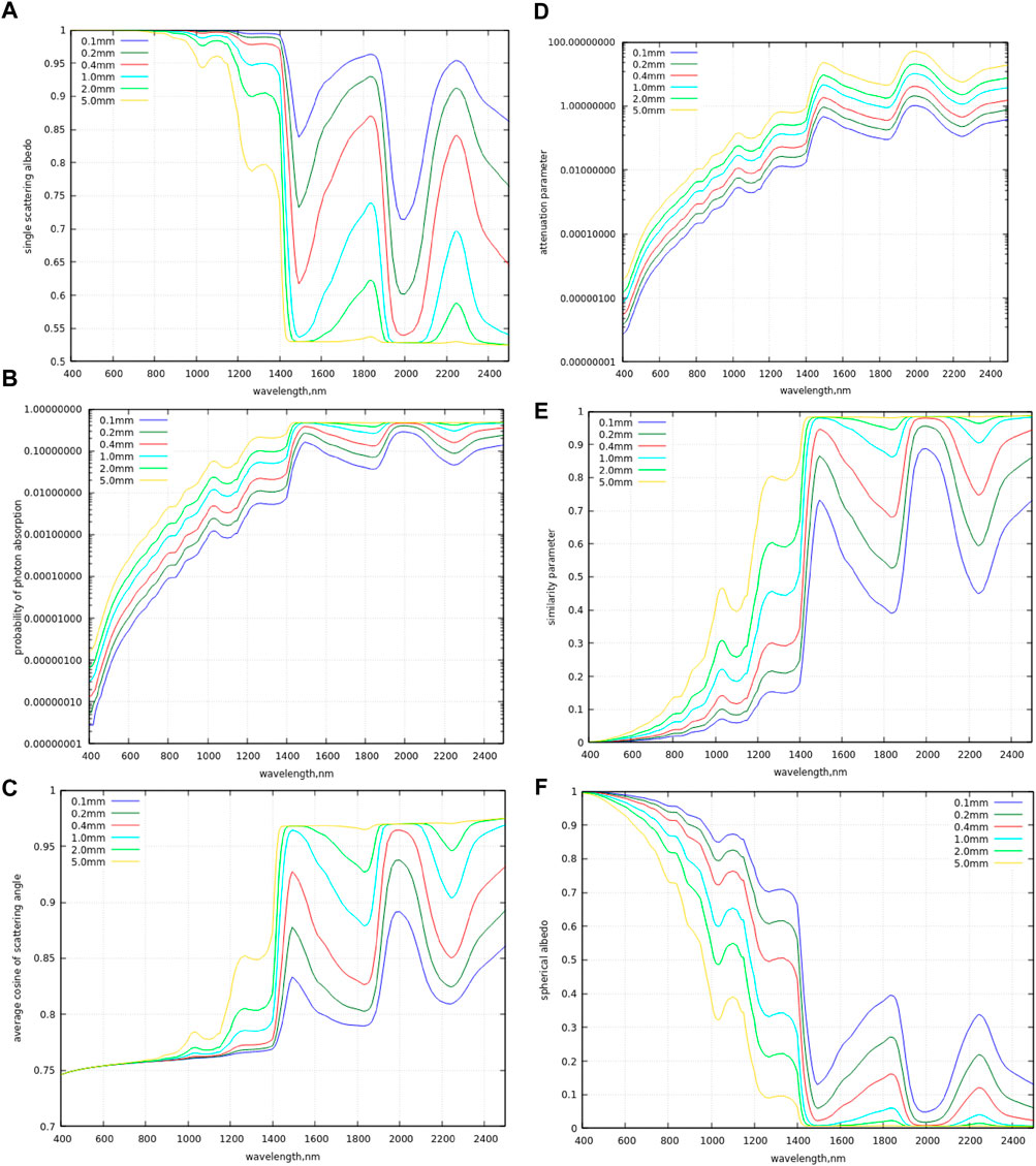
Figure 2. Dependence of SSA (A), PPA (B), average cosine of scattering angle (C), attenuation parameter (D), similarity parameter (E), and spherical albedo (F) on the wavelength for various effective diameters of snow grains.
The snow spectral nadir reflectance is shown in Figure 3. The calculations have been performed using the approximate forward model presented above at various values of the parameters (
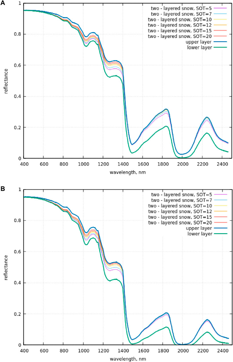
Figure 3. (A) Spectral dependence of the reflectance calculated using the LART model (Eqs 1–10 (Yanovitskij, 1997; Kokhanovsky et al., 2024; Weinhart et al., 2020)) for several values of snow optical thickness. The results for the semi-infinite snow with the parameters of the upper and lower layers are also given. The observation is in the nadir direction, and the solar zenith angle is equal to 60°. (B) The same as in (A), except the diameters of the upper and lower snow layers are two times larger.
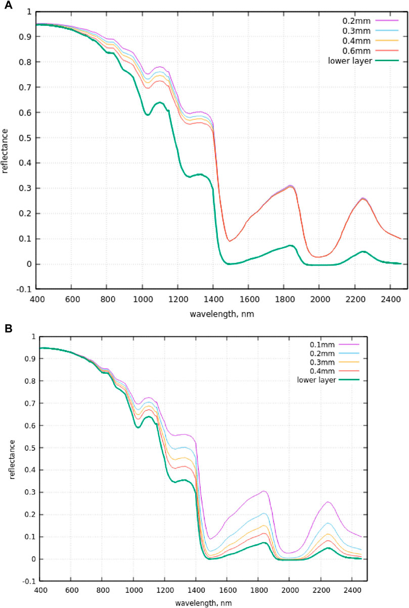
Figure 4. (A) The same as in Fig.3, except for a snow optical thickness of 10, the diameter of ice grains in the upper layer is 0.1 mm and variable diameters of ice grains in the lower layer are in the 0.2–0.6 mm range, as shown in the figure. The calculations for the case of a homogeneous layer of ice grains with a diameter of 0.6 mm are given by the lower green line. (B) The same as in (A), except that the diameter of ice grains in the upper layer is equal to 0.1, 0.2, 0.3, and 0.4 mm and the diameter of ice grains in the lower layer is equal to 0.6 mm. The calculations for the case of a homogeneous layer of ice grains with a diameter of 0.6 mm are given by the lower green line.
The task of the inverse problem is to derive the parameters of the model specified above (namely,
Now, instead of the assumed three coefficients, we have just two (
where
where
Furthermore, we note that the solar light at the wavelength
The answer is
On the other hand, the following is derived using Eq. 2 for the wavelength
where
where
In the next step, we find the values of
where
After finding the pair
This equation follows directly from Eqs 1, 7. The values of
where
Eq 37 has the following physical solution:
Therefore, the optical thickness of the upper snow layer is
In the final step, we make the last iteration to find the updated value of
The determination of the parameters
If needed, the plane and spherical broadband albedo can also be derived by integrating Eqs 44, 45 with respect to the wavelength (Kokhanovsky, 2021). In the case of layered snow, this procedure will lead to more accurate values of the spectral reflectance above 1,400 nm, and therefore, more accurate values of the broadband albedo will be derived. The same is true for the snow absorptance at diffuse
We have applied the technique described above to the 30 × 30 km area around the Concordia Research Station (75.09978 S, 123.332196 E) in Antarctica. The EnMAP measurements were performed on 21 December 2023 (00:47:46 UTC, 08:47:46 UTC local time). The station is located on the Antarctic Plateau at a height of 3.2 km above sea level. The EnMAP L1C radiance data have been used. The radiance has been transformed into reflectance, as explained by Kokhanovsky et al. (2023).
The meteorological parameters at the ground derived from a Vaisala WXT520 weather station installed above the Physics shelter, Concordia Station (http://refir.fi.ino.it/rtDomeC/), are presented in Figure 5A. In particular, one can see that the air temperature is
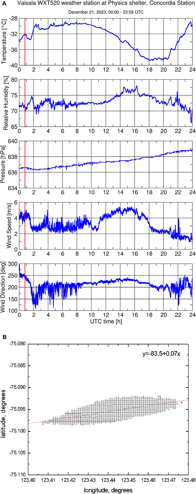
Figure 5. (A) Meteorological parameters at the ground. (B) Wind direction estimated from EnMAP measurements. The coefficient
The measured spectral top-of-atmosphere reflectance at the three channels used in the retrievals is shown in Figure 6. The station is clearly seen in all maps given in Figure 6. The track leading to the station is visible in the maps at 1,026 and 1,235 nm. This is not the case at 2,233 nm, which could be related to the fact that the track is covered by the fresh snow layer and that the radiation at this wavelength hardly penetrates the snow depth at which the track is located.
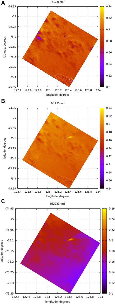
Figure 6. (A) Reflectance R (1,026 nm) map. (B) Reflectance R (1,235 nm) map (C). Reflectance R (2,233 nm) map.
The measured and fitting spectral reflectances (for the assumed single semi-infinite snow layer and a two-layered snowpack) at the location (74.9759 S, 123.0508 E, upper left corner in Figure 6A) are shown in Figure 7A. The calculations for the single semi-infinite snow layer have been done using Eq. 12. The value of the diameter of ice grains
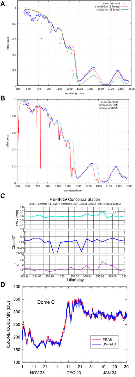
Figure 7. (A) Measured snow spectral reflectance in the nadir direction. The results of numerical simulations according to the developed forward model for single- and two-layered snow are also shown. The solar zenith angle is 56°. (B) Measured snow spectral reflectance in the nadir direction. The results of numerical simulations according to the developed forward model for the TOA and BOA spectral reflectances in the case of a two-layered snowpack are also shown. The solar zenith angle is 56°. (C). The temporal variation of the PWV at the Concordia station. The vertical line corresponds to the time of measurement. The detected cloud optical thickness (cloud OT) is below 0.1. The lower panel shows the accuracy of fit used for the determination of the PWV. (D). The variation in the total ozone derived from ground measurements (UV-RAD) and ERA5 (https://www.ecmwf.int/en/forecasts/dataset/ecmwf-reanalysis-v5) at the Concordia Research Station. ERA5 is the fifth generation of the European Center for Medium-range Weather Forecasts (ECMWF) atmospheric reanalysis of the global climate, covering the period from January 1940 to the present. The rapid fluctuations of the TOC at the time of EnMAP measurements (December 21, 00:47:46 UTC) are clearly seen.
We also simulated the TOA EnMAP spectrum using the modified version of the radiative transfer model SNOWTRAN (Kokhanovsky et al., 2024). In particular, the LART model described in this work has been incorporated into the SNOWTRAN model. The results are given in Figure 7B, where we used the values of the precipitable water vapor PWV = 0.6 mm measured on the ground using the technique described by Kokhanovsky et al. (2024) (see Fig. 7c). The total ozone column was assumed to be equal to 360DU, which is close to the ground-measured value of total ozone (338DU). The radiometer used for the ground measurements of the total ozone is described by Kokhanovsky et al. (2024). We have found that the assumed value of the total ozone column (7% higher value as measured on the ground) better describes EnMAP observations, which is possibly due to some differences in the location of the EnMAP ground scene with a spectrum shown in Figure 7A and the location of the instrument. The fluctuations in the temporal variation of the total ozone (see Figure 7D) and errors in ground measurements could also contribute to this difference.
Figure 7B shows that the measured and simulated TOA spectra are close to each other. This leads to the conclusion that the radiative transfer in the atmosphere-underlying surface system over the area around the Concordia Research Station is well-understood. The accurate performance of the EnMAP mission over bright surfaces is confirmed. Both TOC and PWV can be retrieved from ENMAP measurements, as demonstrated by Kokhanovsky et al. (2024) and confirmed by Figure 7B. The aerosol load in the area close to the station is very low due to the absence of atmospheric pollution sources and the high elevation of the station. Light scattering by molecules is far more important at this location than that by atmospheric aerosols. We have assumed that the aerosol optical thickness at 550 nm is 0.01 and the Angström exponent is equal to 1.6, which is typical for the aerosol over the Concordia Research Station (Six et al., 2005).
The maps of the retrieved snow characteristics are given in Figure 8. The respective statistical characteristics of the retrieved parameters are presented in Table 1. The average value of
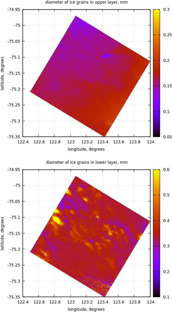
Figure 8. Ice grain size in the upper (upper picture) and lower (lower picture) snow layers.
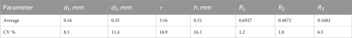
Table 1. Average value and the coefficient of variance (CV = standard deviation/mean) of various snow characteristics. The last three columns show the average values of the spectral reflectances at wavelengths 1,026, 1,235, and 2,233 nm.
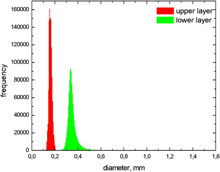
Figure 9. Statistical distributions of the derived snow diameters in the upper and lower snow layers.
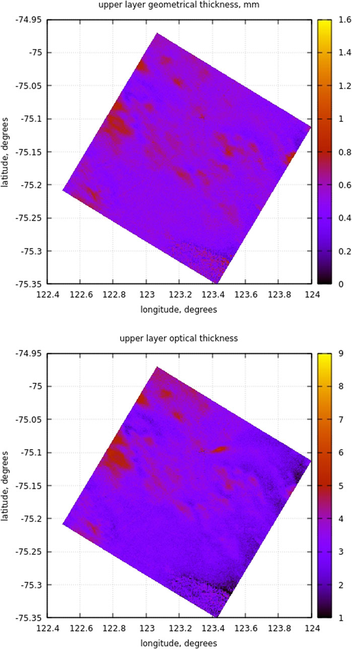
Figure 10. Geometrical (upper panel) and optical (lower panel) upper snow layer thickness.
The estimation of the snow parameters can be performed only in the absence of clouds and pollution sources on the ground. Therefore, the derived results at the location of the plume from the station do not represent the properties of the underlying surface. In particular, Figure 8 (upper panel) shows that the sizes of particles in the exhaust plume are smaller than those of the particles on the ground as one might expect.
In addition to the snow grain size, we have derived the snow-specific surface area
The spatial distribution of the specific surface area in the upper layer is shown in Figure 11. The average value is 40
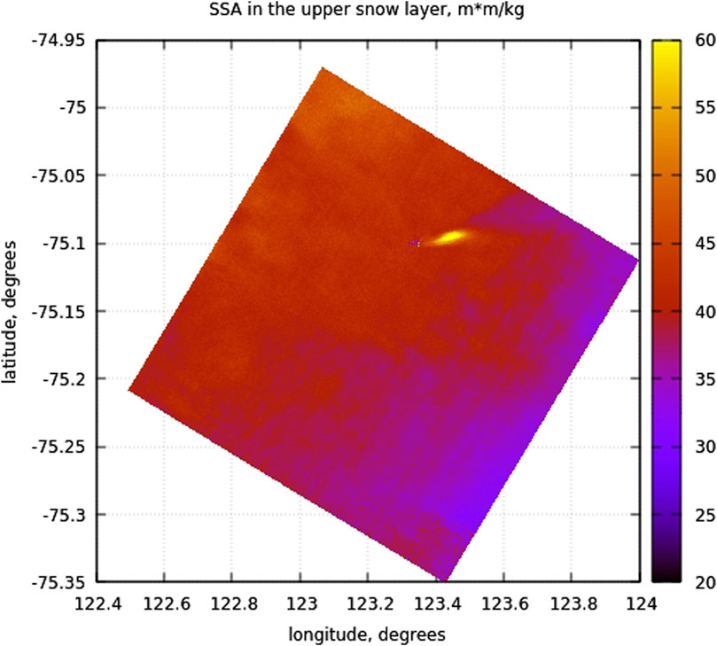
Figure 11. Snow-specific surface area in the upper snow layer.
It has been reported (Inoue et al., 2024) that the snow-specific surface area along the traverse road from the coast to Dome Fuji, Antarctica, was
We have proposed the fast and simple, fully analytical LART model for the calculation of the BOA and TOA spectral reflectance over layered snow surfaces in the VNIR and SWIR regions of the electromagnetic spectrum. It has been assumed that the snow is an ideally horizontal surface without sastrugi and any inclination. The close-packed media effects have been neglected. The ice particles have been modeled as Koch fractals of the second generation (Kokhanovsky, 2021). We have accounted for the light absorption by atmospheric gases such as molecular oxygen, water vapor, and ozone. The vertical inhomogeneity of the snow surface has been accounted for by assuming a two-layered snow model. We have supposed that the upper layer is optically thick and the lower layer is semi-infinite. The derived technique has been applied to EnMAP data, which show the capability of detecting thin fresh snow layers overlying aged snow using the capability of the EnMAP to measure the solar light reflectance from snow in the SWIR. Therefore, in this work, we have confirmed the possible existence of a thin upper snow layer with tiny ice crystals on the Antarctic plateau postulated by Grenfell et al. (1994) and further studied by Turner et al. (2019). This layer, being geometrically thin, has important impacts on the radiative budget in the SWIR region of the electromagnetic spectrum, leading to a larger reflectance of electromagnetic radiation from snow in the SWIR than in the case of a homogeneous layer with the grain size of the aged snow underneath.
The determination of snow characteristics using only VNIR measurements may lead to biases in the retrieved snow grain sizes and, therefore, snow albedo, which is an essential climate variable. The derived technique can be used in the improvement of spaceborne spectral and broadband albedo determination using satellite measurements, as well as for the detection and characterization of fresh snowfall events using EnMAP and other hyperspectral datasets. The EnMAP data can also be used to retrieve the values of TOC, PWV, and the direction of the wind on the ground in cases where strong aerosol emission sources are present on the ground.
We believe that the model proposed in this work will be useful for the determination of snow parameters using other hyperspectral and multispectral instrumentation, including ground-based optical spectrometers and radiometers. The technique can be easily generalized to study other optically thick turbid media with large scatterers, including soil and desert surfaces.
Future work will focus on the validation of the derived parameters, the estimation of uncertainties in retrievals, and the runs of the model for various regions and seasons.
The raw data supporting the conclusions of this article will be made available by the authors, without undue reservation.
AK: conceptualization, data curation, formal analysis, investigation, methodology, software, validation, visualization, writing–original draft, and writing–review and editing. MB: data curation, writing–review and editing. KS: project administration, resources, software, supervision, writing–review and editing. DE: formal analysis, investigation, software, writing–original draft, and writing–review and editing. BP: conceptualization, data curation, formal analysis, investigation, writing–original draft, and writing–review and editing. GB: conceptualization, data curation, formal analysis, investigation, methodology, visualization, writing–original draft, and writing–review and editing. RS: methodology, writing–original draft. SC: project administration, resources, supervision, methodology, investigation, writing–original draft.
The author(s) declare that no financial support was received for the research, authorship, and/or publication of this article. The research was funded by the EnMAP mission science program funded within the German Earth observation program by the DLR Space Agency with resources from the German Federal Ministry for Economic Affairs and Climate Action (grant numbers 50EE1923 and 50EE2401).
The authors thank DLR for providing EnMAP data and ECMWF for providing ERA5 re-analysis data.
The authors declare that the research was conducted in the absence of any commercial or financial relationships that could be construed as a potential conflict of interest.
The author(s) declared that they were an editorial board member of Frontiers, at the time of submission. This had no impact on the peer review process and the final decision.
All claims expressed in this article are solely those of the authors and do not necessarily represent those of their affiliated organizations, or those of the publisher, the editors, and the reviewers. Any product that may be evaluated in this article, or claim that may be made by its manufacturer, is not guaranteed or endorsed by the publisher.
Afanas’ev, V. P., Basov, A. Y., Budak, V. P., Efremenko, D. S., and Kokhanovsky, A. A. (2020). Analysis of the discrete theory of radiative transfer in the coupled “ocean–atmosphere” system: current status, problems and development prospects. J. Mar. Sci. Eng. 8 (3), 202. doi:10.3390/jmse8030202
Brent, R. P. (1973). Algorithms for Minimization without Derivatives. Englewood Cliffs, NJ: Prentice-Hall.
Chuprov, I., Konstantinov, D., Efremenko, D., Zemlyakov, V., and Gao, J. (2022). Solution of the radiative transfer equation for vertically inhomogeneous media by numerical integration solvers: comparative analysis. Light and Eng., 21–30. doi:10.33383/2022-030
Efremenko, D., Doicu, A., Loyola, D., and Trautmann, T. (2013). Acceleration techniques for the discrete ordinate method. J. Quantitative Spectrosc. Radiat. Transf. 114, 73–81. doi:10.1016/j.jqsrt.2012.08.014
Efremenko, D., Molina García, V., Gimeno García, S., and Doicu, A. (2017). A review of the matrix-exponential formalism in radiative transfer. J. Quantitative Spectrosc. Radiat. Transf. 196, 17–45. doi:10.1016/j.jqsrt.2017.02.015
Gallet, J.-C., Domine, F., Arnaud, L., Picard, G., and Savarino, J. (2011). Vertical profile of the specific surface area and density of the snow at Dome C and on a transect to Dumont D'Urville, Antarctica – albedo calculations and comparison to remote sensing products. Cryosphere 5, 631–649. doi:10.5194/tc-5-631-2011
Gay, M., Fily, M., Genthon, C., Frezzotti, M., Oerter, H., and Winther, J.-G. (2002). Snow grain size measurements in Antarctica. J. Glaciol. 48, 527–535. doi:10.3189/172756502781831016
Grenfell, T. C., Warren, S. G., and Mullen, P. C. (1994). Reflection of solar radiation by the Antarctic snow surface at ultraviolet, visible, and near-infrared wavelengths. J. Geophys. Res. 99 (D9), 18669–18684. doi:10.1029/94jd01484
Guanter, L., Kaufmann, H., Segl, K., Foerster, S., Rogass, C., Chabrillat, S., et al. (2015). The EnMAP spaceborne imaging spectroscopy mission for Earth Observation. Remote Sens. 7, 8830–8857. doi:10.3390/rs70708830
Henyey, L. G., and Greenstein, J. L. (1941). Diffuse radiation in the Galaxy. Astrophysical J. 93, 70–83. doi:10.1086/144246
Hu, Y.-X., Wielicki, B., Lin, B., Gibson, B., Tsay, S.-C., Stamnes, K., et al. (2000). δ-Fit: a fast and accurate treatment of particle scattering phase functions with weighted singular-value decomposition least-squares fitting. J. Quantitative Spectrosc. Radiat. Transf. 65 (4), 681–690. doi:10.1016/s0022-4073(99)00147-8
Inoue, R., Aoki, T., Fujita, S., Tsutaki, S., Motoyama, H., Nakazawa, F., et al. (2024). Spatiotemporal variation in the specific surface area of surface snow measured along the traverse route from the coast to Dome Fuji, Antarctica. EGUsphere. doi:10.5194/egusphere-2024-769
Kokhanovsky, A., Brell, M., Segl, K., and Chabrillat, S. (2024). SNOWTRAN: a fast radiative transfer model for polar hyperspectral remote sensing applications. Remote Sens. 16, 334. doi:10.3390/rs16020334
Kokhanovsky, A., Di Mauro, B., Garzonio, R., and Colombo, R. (2021). Retrieval of dust properties from spectral snow reflectance measurements. Front. Environ. Sci. 9. doi:10.3389/fenvs.2021.644551
Kokhanovsky, A., Lamare, M., Danne, O., Brockmann, C., Dumont, M., Picard, G., et al. (2019). Retrieval of snow properties from the sentinel-3 ocean and land colour instrument. Remote Sens. 11, 2280. doi:10.3390/rs11192280
Kokhanovsky, A., and Rozanov, V. V. (2012). Droplet vertical sizing in warm clouds using passive optical measurements from a satellite. Atmos. Meas. Tech. 5, 517–528. doi:10.5194/amt-5-517-2012
Kokhanovsky, A. A., Brell, M., Segl, K., Bianchini, G., Lanconelli, C., Lupi, A., et al. (2023). First retrievals of surface and atmospheric properties using EnMAP measurements over Antarctica. Remote Sens. 15, 3042. doi:10.3390/rs15123042
Li, W., Stamnes, K., Chen, B., and Xiong, X. (2011). Snow grain size retrieved from near-infrared radiances at multiple wavelengths. Geophys. Res. Let. 28 (9), 1699–1702. doi:10.1029/2000gl011641
Mishchenko, M. I., Dlugach, J. M., Yanovitskij, E. G., and Zakharova, N. T. (1999). Bidirectional reflectance of flat, optically thick particulate layers: An efficient radiative transfer solution and applications to snow and soil surfaces. J. Quantitative Spectrosc. Radiat. Transf. 63, 409–432. doi:10.1016/s0022-4073(99)00028-x
Nakajima, T., and Tanaka, M. (1988). Algorithms for radiative intensity calculations in moderately thick atmospheres using a truncation approximation. J. Quantitative Spectrosc. Radiat. Transf. 40 (1), 51–69. doi:10.1016/0022-4073(88)90031-3
Sato, N., Kikuchi, K., Barnard, S. C., and Hogan, A. W. (1981). Some characteristic properties of ice crystal precipitation in the summer season at South Pole station, Antarctica. J. Meteorol. Soc. Jpn. 59, 7772–7780. doi:10.2151/jmsj1965.59.5_772
Six, D., Fily, M., Blarel, L., and Goloub, P. (2005). First aerosol optical thickness measurements at Dome C (East Antarctica), summer season 2003–2004. Atmos. Environ. 39, 5041–5050. doi:10.1016/j.atmosenv.2005.05.010
Storch, T., Honold, H.-P., Chabrillat, S., Habermeyer, M., Tucker, P., Brell, M., et al. (2023). The EnMAP imaging spectroscopy mission towards operations. Rem. Sens. Env. 294, 113632. doi:10.1016/j.rse.2023.113632
Turner, J., Phillips, T., Thamban, M., Rahaman, W., Marshall, G. J., Wille, J. D., et al. (2019). The dominant role of extreme precipitation events in Antarctic snow fall variability. Geophys. Res. Let. 46, 3502–3511. doi:10.1029/2018gl081517
van de Hulst, H. C. (1974). The spherical albedo of a planet covered with a homogeneous cloud layer. Astron. Astrophys. 35, 209–214.
Warren, S., and Brand, R. E. (2008). Optical constants of ice from the ultraviolet to the microwave: a revised compilation. J. Geophys. Res. 113, D14. doi:10.1029/2007jd009744
Weinhart, A. H., Freitag, J., Hörhold, M., Kipfstuhl, S., and Eisen, O. (2020). Representative surface snow density on the East Antarctic plateau. Cryosphere 14, 3663–3685. doi:10.5194/tc-14-3663-2020
Wiscombe, W. J. (1977). The Delta–M Method: rapid yet accurate radiative flux calculations for strongly asymmetric phase functions. J. Atmos. Sci. 34 (9), 1408–1422. doi:10.1175/1520-0469(1977)034<1408:tdmrya>2.0.co;2
Keywords: cryosphere and climate, radiative transfer, light scattering, snowfall detection, ice crystals, remote sensing
Citation: Kokhanovsky A, Brell M, Segl K, Efremenko D, Petkov B, Bianchini G, Stone R and Chabrillat S (2024) The two-layered radiative transfer model for snow reflectance and its application to remote sensing of the Antarctic snow surface from space. Front. Environ. Sci. 12:1416597. doi: 10.3389/fenvs.2024.1416597
Received: 12 April 2024; Accepted: 19 June 2024;
Published: 26 July 2024.
Edited by:
Zhongqiu Sun, Northeast Normal University, ChinaReviewed by:
Tomonori Tanikawa, Japan Meteorological Agency, JapanCopyright © 2024 Kokhanovsky, Brell, Segl, Efremenko, Petkov, Bianchini, Stone and Chabrillat. This is an open-access article distributed under the terms of the Creative Commons Attribution License (CC BY). The use, distribution or reproduction in other forums is permitted, provided the original author(s) and the copyright owner(s) are credited and that the original publication in this journal is cited, in accordance with accepted academic practice. No use, distribution or reproduction is permitted which does not comply with these terms.
*Correspondence: Alexander Kokhanovsky, a29raGFub3ZAZ2Z6LXBvdHNkYW0uZGU=; Robert Stone, cm9ic3RlcGhzdG9uQGdtYWlsLmNvbQ==; Sabine Chabrillat, Y2hhYnJpQGdmei1wb3RzZGFtLmRl
Disclaimer: All claims expressed in this article are solely those of the authors and do not necessarily represent those of their affiliated organizations, or those of the publisher, the editors and the reviewers. Any product that may be evaluated in this article or claim that may be made by its manufacturer is not guaranteed or endorsed by the publisher.
Research integrity at Frontiers
Learn more about the work of our research integrity team to safeguard the quality of each article we publish.