Novel spatio-temporal attention causal convolutional neural network for multi-site PM2.5 prediction

Multi-site PM2.5 prediction has emerged as a crucial approach, given that the accuracy of prediction models based solely on data from a single monitoring station may be constrained. However, existing multi-site PM2.5 prediction methods predominantly rely on recurrent networks for extracting temporal dependencies and overlook the domain knowledge related to air quality pollutant dispersion. This study aims to explore whether a superior prediction architecture exists that not only approximates the prediction performance of recurrent networks through feedforward networks but also integrates domain knowledge of PM2.5. Consequently, we propose a novel spatio-temporal attention causal convolutional neural network (Causal-STAN) architecture for predicting PM2.5 concentrations at multiple sites in the Yangtze River Delta region of China. Causal-STAN comprises two components: a multi-site spatio-temporal feature integration module, which identifies temporal local correlation trends and spatial correlations in the spatio-temporal data, and extracts inter-site PM2.5 concentrations from the directional residual block to delineate directional features of PM2.5 concentration dispersion between sites; and a temporal causal attention convolutional network that captures the internal correlation information and long-term dependencies in the time series. Causal-STAN was evaluated using one-year data from 247 sites in mainland China. Compared to six state-of-the-art baseline models, Causal-STAN achieves optimal performance in 6-hour future predictions, surpassing the recurrent network model and reducing the prediction error by 8%–10%.

1 Introduction

Air pollution has emerged as a significant challenge to environmental sustainability in the 21st century. Specifically, PM2.5 increasingly impacts urban health and the quality of life of residents negatively (Yan et al., 2022). Chronic exposure to PM2.5 may elevate the risk of non-communicable respiratory diseases, cardiovascular diseases, and diabetes (Yang et al., 2022). Additionally, short-term exposure to PM2.5 has been shown to accelerate aging, as evidenced by changes in DNA methylation profiles associated with blood coagulation, oxidative stress, and systemic inflammation (Gao et al., 2022). Consequently, PM2.5 prediction studies hold significant importance and are considered a critical issue for environmental protection (Ai et al., 2019). However, current methods that predict PM2.5 concentrations using data from a single monitoring station fall short in capturing spatial correlations among stations, thereby limiting their predictive accuracy. Therefore, the development of a multi-site PM2.5 prediction approach that harnesses spatial relationships between air quality monitoring stations is crucial. Such an approach would not only broaden the scope of PM2.5 concentration predictions but also enhance the accuracy of these models, providing stronger support for effective air quality management strategies and improving public health protection (Wang et al., 2023).

Over the past few decades, PM2.5 prediction models have evolved from traditional physical and statistical models to more sophisticated machine learning and deep learning approaches. Traditional physical models have primarily been focused on simulating the dispersion, deposition, and chemical reactions of PM2.5 processes (Marvin et al., 2022). For instance, the WRF/Chem model forecasts environmental conditions by assessing the potential physicochemical impacts and dynamics of pollutants (Grell et al., 2005). However, these models’ reliance on complex data structures and limited generalization ability present significant challenges for practical applications (Liu and Chen, 2020). Common statistical models employed in PM2.5 prediction include multiple linear regression (MLR) (Lagesse et al., 2020), autoregressive integrated moving average (ARIMA) (Wang et al., 2017), and autoregressive conditional heteroskedasticity (ARCH) (Wu and Kuo, 2012). A primary limitation of these models is their reliance on linear assumptions, which often fails to capture the inherently nonlinear behavior of PM2.5, thus compromising their predictive accuracy (Marsha and Larkin, 2019; Erden, 2023). In contrast, machine learning models excel in capturing nonlinear patterns, thus proving highly effective in PM2.5 prediction. These models harness complex data patterns and relationships, enhancing prediction accuracy by addressing the nonlinearity of PM2.5 concentrations (Wang et al., 2024b). Notable examples include support vector machines (SVM) (Lai et al., 2021), extreme gradient boosting (XGBoost) (Liu et al., 2021), random forest (Chen et al., 2023), and various integration techniques (Sun et al., 2023; Teng et al., 2023; Liu et al., 2024). However, despite their capabilities, many machine learning approaches primarily focus on single-station predictions and often neglect the spatial interactions and distributions among multiple monitoring stations, which limits their effectiveness in comprehensive urban air quality management (de Hoogh et al., 2018).

With advancements in deep learning, researchers are increasingly exploring multi-site PM2.5 forecasting nationwide. Convolutional Neural Networks (CNNs) are pivotal in extracting spatial correlation features from time series, initially recognizing spatial correlations between adjacent values, then leveraging convolutional operators to augment learning processes (Faraji et al., 2022). Recurrent Neural Networks (RNNs), known for sequence modeling, utilize a hidden state vector updated sequentially with each input, facilitating temporal information transmission across time steps (Young et al., 2018). These attributes make RNNs suitable for time series prediction tasks, including PM2.5 forecasting (Shakya et al., 2023). Given that multi-site PM2.5 prediction requires mastering spatio-temporal sequences, hybrid models combining CNNs and RNNs have become prevalent. These models employ CNNs to delineate spatial correlations between stations, while RNNs handle the temporal dynamics of PM2.5 concentrations at individual stations (Chiang and Horng, 2021; Du et al., 2021; Zhang et al., 2022; Teng et al., 2023). However, despite their advantages, RNNs encounter significant challenges in managing long series and large-scale multi-site forecasting due to their limitations in parallel processing and capturing distant dependencies, as highlighted by Liang and Tang (2022), along with others (Vaswani et al., 2017; Khandelwal et al., 2018). To address these limitations, recent studies have focused on developing novel feedforward models that better accommodate the complexities of multi-site PM2.5 prediction (Chinatamby and Jewaratnam, 2023).

Recent advances in multi-site PM2.5 prediction have increasingly focused on innovative feedforward models, notably those employing Temporal Convolutional Networks (TCNs) and attention mechanisms. The significant advantage of TCNs in time series prediction is attributed to their straightforward structure, extensive expansion flexibility, and clear causal constraints (Bi et al., 2022; Li et al., 2022; Nasr Azadani and Boukerche, 2022). For example, Zhang et al. (2021) designed a causal convolutional neural network for short-term PM2.5 prediction using TCNs, whose convolution operation explicitly takes causality into account, i.e., the output of a time step only depends on the same or earlier time steps in the previous layer, providing a new perspective on PM2.5 feedforward prediction modeling. However, TCNs struggles to capture the dependency of distant locations in the time series and to extract the internal correlation information of the input data. The Airformer, recently introduced by Liang et al. (2023), stands as a notable model founded on the attention mechanism for air quality prediction. It depends entirely on this mechanism to discern the spatio-temporal patterns of air quality data and employs the Generation Model and the Inference Model to grasp the inherent uncertainty within the air quality data. While attention-based models demonstrate substantial predictive capabilities, their large size poses practical limitations. Furthermore, the Temporal Convolutional Attention-based Network (TCAN), developed by Hao et al. (2020) for natural language processing tasks, shows promise in sequential task modeling by integrating TCNs with attention mechanisms. However, its application to multi-site PM2.5 prediction is potentially limited by insufficient consideration of spatial correlations among monitoring sites and a lack of domain-specific knowledge on PM2.5 dispersion.

To address the limitations of existing feedforward networks in the task of multi-site PM2.5 prediction, we aim to develop a novel architecture based on feedforward techniques that aspires to reach predictive performance comparable to recurrent networks while improving simplicity and efficiency. Furthermore, the accuracy of multi-site PM2.5 predictions not only depends on advanced modeling techniques but also requires a deep understanding of domain-specific knowledge about the pollutant, such as the direction of pollutant dispersion during events (Wang et al., 2020; Zhou et al., 2021). It is crucial to integrate this knowledge into the prediction models to improve accuracy.

Based on these objectives, this study introduces a novel exploratory architecture: the spatio-temporal attention causal convolutional neural network (Causal-STAN) for multi-site PM2.5 prediction. First, we propose a multi-site spatio-temporal feature integration module. This module employs a CNN to identify temporal local correlation trends and spatial correlations in spatio-temporal data, integrates domain knowledge of PM2.5 pollutant dispersion, and introduces a directional residual block to extract directional features of PM2.5 concentration dispersion between sites. Second, we designed a temporal causal attention convolutional network, inspired by TCAN, that simulates the input causality of RNNs using dilated causal convolution. This network incorporates an attention mechanism to effectively capture the internal correlation information and long-term dependencies within PM2.5 time series. We aim to achieve an approximate replacement of RNNs with temporal causal attention convolutional network and assess the efficacy of the networks’ unique “causal” properties in the PM2.5 prediction task. To assess the proposed method’s effectiveness, experiments were conducted with data from 247 air quality monitoring stations across 41 cities in the Yangtze River Delta region of China. The main contributions are as follows.

(1) Addressing the scarcity of concise and efficient feedforward prediction models in PM2.5 prediction, this study introduces a novel spatio-temporal attention causal convolutional neural network (Causal-STAN) tailored for multi-site PM2.5 concentration prediction.

(2) Incorporating domain knowledge of air pollutant dispersion, a directional residual block was designed and integrated into the multi-site spatio-temporal feature integration module, enabling the extraction of directional features of inter-site PM2.5 concentration dispersion.

(3) Maximum information coefficients are employed to simultaneously detect similar sites processed by the proposed model, facilitating the extraction of comprehensive knowledge from the dataset.

(4) Performance evaluation results demonstrate that the proposed multi-site PM2.5 feedforward prediction model offers significant advantages over the baseline model, surpassing even the recurrent models in comparison. This model presents a viable alternative to RNNs for multi-site PM2.5 prediction tasks, showcasing its potential effectiveness.

2 Materials and methods

2.1 Study area and data collection

Data for this study were sourced from 247 air quality monitoring stations, spanning the period 1 January 2022, to 31 December 2022, across the Yangtze River Delta region of China, encompassing 41 cities. Figure 1 illustrates the geographical distribution of all study monitoring stations. Hourly data from each monitoring station were compiled into a one-dimensional eigenvector, incorporating pollutant data, meteorological data, and the air quality index (AQI). Pollutant data and AQI were sourced from the urban air quality real-time publishing platform of the China National Environmental Monitoring Center¹, amounting to 4,327,440 records. Meteorological data were acquired from the National Climatic Data Center², totaling 1,078,423 records. Detailed data specifications are provided in Table 1. Since the meteorological stations and air pollutant monitoring stations are not directly matched, we selected meteorological data from the nearest meteorological station (based on Euclidean distance) for each pollutant monitoring station. This approach ensures that the meteorological data closely reflect local environmental conditions.

Figure 1

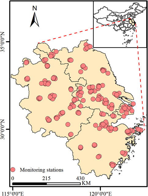
Figure 1. Geographical distribution of the 247 air quality monitoring stations across 41 cities in the Yangtze River Delta region, China.

Table 1

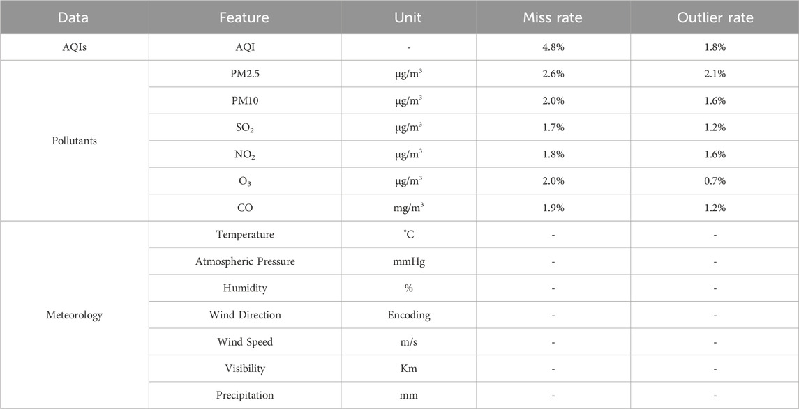
Table 1. Description of dataset in this study, the last two columns show the missing and outlier rates for the pollutant indicators in the dataset, respectively.

2.2 Data preprocessing

Air quality data collected by the urban air quality real-time publishing platform of the China National Environmental Monitoring Center exhibit a certain percentage of missing values and outliers. Missing values and outliers can result from prolonged operation of monitoring equipment or exposure to extreme weather conditions, such as heavy rain, storms, and haze. Table 1 presents the rates of missing and outlier values for pollutant data and AQI in the dataset, indicating a higher incidence of missing values for AQI. In this study, outliers were detected using the interquartile range (IQR) method, defined as the difference between the third quartile (Q3) and the first quartile (Q1). The upper outlier limit is calculated as Q3 plus 1.5 times the IQR, and the lower limit is Q1 minus 1.5 times the IQR. Data identified as outliers are subsequently replaced with missing values. To address the missing values in the dataset, two-way linear interpolation was employed for imputation.

2.3 Spatio-temporal correlation analysis

Considering the evident spatio-temporal correlation of PM2.5 across various monitoring stations, constructing a model based solely on historical data from a single station may present limitations. To enhance the accuracy of model predictions, it is imperative to integrate data from multiple monitoring stations for spatio-temporal correlation analysis. For a dataset with historical data from N monitoring stations, input data are transformed into a three-dimensional tensor $\mathit{X}\in {\mathit{R}}^{\mathit{N}\times \mathit{T}\times \mathit{F}}$, where T denotes the time step and F denotes the number of features associated with PM2.5. For any given target site, the initial step involves determining the correlation between its time series data and that of other sites.

The maximum information coefficient (MIC) is a nonparametric statistical method that measures the correlation between two variables, as proposed by Reshef et al. (2011). The MIC is defined as shown in Equations 1, 2:

$\mathit{I}\left(\mathit{x},\mathit{y}\right)=\int \mathit{p}\left(\mathit{x},\mathit{y}\right){\mathit{log}}_{\mathbf{2}}\frac{\mathit{p}\left(\mathit{x},\mathit{y}\right)}{\mathit{p}\left(\mathit{x}\right)\mathit{p}\left(\mathit{y}\right)}\mathit{d}\mathit{x}\mathit{d}\mathit{y}(1)$

$\mathit{M}\mathit{I}\mathit{C}\left(\mathit{x},\mathit{y}\right)=\underset{\mathit{a}\times \mathit{b}<\mathit{B}}{\mathit{max}}\frac{\mathit{I}\left(\mathit{x},\mathit{y}\right)}{{\mathit{log}}_{\mathbf{2}}\mathit{min}\left(\mathit{a},\mathit{b}\right)}(2)$

where x and y are two random variables, and a and b are the number of bins into which the x and y-axes are divided, respectively. B is a parameter whose size is approximately the 0.6 power of the sample size (Zhu et al., 2021). MIC values range from 0 to 1, where 0 indicates no correlation and 1 indicates a perfect correlation. Unlike traditional methods such as the Pearson correlation coefficient, the MIC is capable of capturing more complex nonlinear relationships and offers greater robustness (Wang et al., 2024a). We employ MIC to quantify interactions between sites and effectively capture nonlinear relationships between variables, as shown in Equation 3:

$\mathit{\theta }\left({\mathit{Y}}_{*},{\mathit{Y}}_{\mathit{i}}\right)=\mathit{M}\mathit{I}\mathit{C}\left({\mathit{Y}}_{*},{\mathit{Y}}_{\mathit{i}}\right)(3)$

where ${\mathit{Y}}_{*}$ and ${\mathit{Y}}_{\mathit{i}}$ represent the PM2.5 time series of the current target site and the ith site among all study sites, respectively; $\mathit{\theta }\left({\mathit{Y}}_{*},{\mathit{Y}}_{\mathit{i}}\right)$ the numerical value of correlation.

Upon obtaining the correlation values between the current target site and all other sites, these values are compiled into a correlation vector, as shown in Equation 4:

${\mathit{\theta }}_{*}=\left[\mathit{\theta }\left({\mathit{Y}}_{*},{\mathit{Y}}_{\mathbf{1}}\right),\cdots ,\mathit{\theta }\left({\mathit{Y}}_{*},{\mathit{Y}}_{\mathit{i}}\right),\cdots ,\mathit{\theta }\left({\mathit{Y}}_{*},{\mathit{Y}}_{\mathit{N}}\right)\right](4)$

Considering that not all sites significantly impact the target site, setting a correlation threshold to filter out sites with strong interactions with the target site is prudent. As a result, the spatio-temporal correlation analysis produces the final input feature vector as follows, as shown in Equation 5:

${\mathit{X}}_{*}=\left\{{\mathit{X}}_{\mathit{i}}|\mathit{\theta }\left({\mathit{Y}}_{*},{\mathit{Y}}_{\mathit{i}}\right)>{\mathit{\theta }}_{\mathit{t}\mathit{h}},\mathit{i}\in \left\{\mathbf{1},\mathbf{2},\cdots ,\mathit{N}\right\}\right\}(5)$

where ${\mathit{\theta }}_{\mathit{t}\mathit{h}}$ is the set correlation threshold, and ${\mathit{X}}_{*}\in {\mathit{R}}^{\mathrm{C}\times \mathit{T}\times \mathit{F}}$ is the input feature vector for the target site after filtering based on spatio-temporal information. In this vector, C represents the number of monitoring stations that are significantly correlated with the target site, as determined by exceeding the correlation threshold ${\mathit{\theta }}_{\mathit{t}\mathit{h}}$.

2.4 Architecture of the proposed network

The architecture of the proposed Causal-STAN is illustrated in Figure 2, which comprises two main components. The first component is the multi-site spatio-temporal feature integration module, depicted in Figure 2A, while the second component is the temporal causal attention convolutional network, depicted in Figure 2B. The following subsections elaborate on the details of these two components.

Figure 2

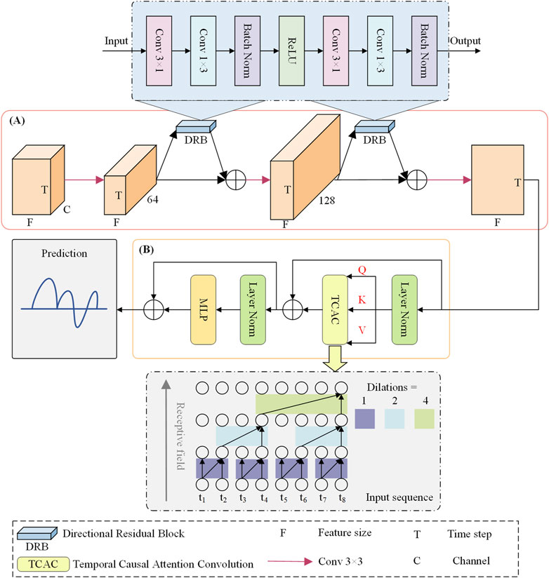
Figure 2. The proposed framework of Causal-STAN, which consists of two components. (A) Multi-site spatio-temporal feature integration module; (B) temporal causal attention convolutional network, which we illustrate using eight time-step examples, here, kernel size = 2, dilation = 1, 2, 4.

2.4.1 Multi-site spatio-temporal feature integration module

Given the input feature ${\mathit{X}}_{*}$, a 3-dimensional vector with spatio-temporal data from various sites, we propose a multi-site spatio-temporal feature integration module to extract spatio-temporal features across sites. The design of this module incorporates the following considerations: 1) Spatio-temporal dependence: Acknowledging the spatial dimension’s significance in spatio-temporal data for feature extraction, we integrate a feature dimension transformation strategy within the convolution operation to enhance the model’s capability to extract spatio-temporal dependent information from various monitoring stations. 2) Directional features of PM2.5 concentration diffusion: With domain knowledge of air pollution diffusion, recognizing that pollutants typically exhibit directional diffusion among stations, affected by environmental factors like wind direction, we designed a directional residual block to capture these directional features.

In Figure 2A, as an example, the first feature at the initial time step has channels corresponding to the number of monitoring sites in ${\mathit{X}}_{*}$. Different target sites may have varying numbers of related sites, denoted by the parameter C, which plays a key role in the prediction model. The number of input channels in the first convolutional layer is set to match the C value of the current target site. This allows the model to dynamically adjust the input channels for each site, optimizing the use of information from related sites. The initial 3 × 3 convolution is used to identify temporal local correlation trends and spatial correlations in the spatio-temporal data, expanding the feature dimension from the specific C value to 64. In other words, the initial 3 × 3 convolution expands the feature dimension of the target site’s feature vector from the specific C value to 64. Subsequently, the directional residual block is introduced with this feature dimension, utilizing longitudinal Conv 3 × 1 and horizontal Conv 1 × 3 convolution kernels to pinpoint pollutants’ spatial spreading characteristics on different axes, thereby improving the model’s detection of potential spatial correlations among sites. Following this, a second 3 × 3 convolution further enhances the extraction of temporally localized correlation trends and spatial correlations, increasing the spatio-temporal data’s feature dimensions to 128. At this juncture, a second directional residual block is applied to the higher-dimensional spatio-temporal data, aiming to learn deeper directional features between sites. Ultimately, a 3 × 3 convolution completes the feature integration, reducing the spatio-temporal data’s feature dimension to 1 and generating a two-dimensional synthesized feature vector as input for the temporal causal attention convolutional network.

The directional residual block uses two convolution operations: a longitudinal 3 × 1 kernel and a horizontal 1 × 3 kernel. These kernels are designed to capture spatial patterns along specific axes, enhancing the model’s ability to analyze pollutant diffusion across the dataset.

2.4.1.1 Longitudinal convolution (3 × 1)

This kernel is structured to extend vertically over three rows in a single column and is configured to extract correlations across different features or sites, analyzing changes along a vertical axis within the data. Such an arrangement is pivotal for identifying site-specific pollution trends or environmental factors that may consistently influence adjacent sites. By targeting vertical slices of data, this convolution adeptly captures dependencies arising from vertical stratification of atmospheric components or variations in emission sources among proximately located sites.

2.4.1.2 Horizontal convolution (1 × 3)

The horizontal kernel, spreading over one row and three columns, is engineered to monitor temporal sequences, enabling the model to trace the evolution of environmental conditions or pollutant levels over time. This kernel excels at detecting patterns across three consecutive time steps, offering insights into how dynamic environmental conditions, such as shifts in wind direction or speed, impact the dispersion and concentration of pollutants.

The outputs from these directional convolutions are integrated using a residual learning framework, where a skip connection adds the block’s input to its output. This method is instrumental in mitigating the vanishing gradient problem commonly encountered in deep neural networks, while also preserving identity information throughout the layers. Such an approach enables the model to refine its predictions by continuously learning from the discrepancies between predicted and actual pollution patterns, significantly enhancing the model’s accuracy and sensitivity to subtle environmental variations.

2.4.2 Temporal causal attention convolutional network

Beyond spatial dependence, a site’s air quality is influenced by its historical data. Given a site’s hidden state ${\mathit{I}}_{\mathbf{1}:\mathit{T}}^{\left(\mathit{L}\right)}\in {\mathit{R}}^{\mathit{T}\times \mathit{F}}$ (output from the spatio-temporal feature integration module) across all past steps, the basic feedforward neural network TCN fails to learn the temporal dependence of distant locations within the sequence and cannot extract the internal correlation information of the inputs. Here, we introduce the temporal causal attention convolutional network as an effective alternative to the standard TCN for temporal modeling. As shown in Figure 2B, the key part of the proposed network is the temporal causal attention convolution, featuring two main modifications:

2.4.2.1 Temporal causal attention

To address TCN’s limitation, we introduce a self-attention mechanism that captures internal time-series relationships and long-range dependencies. Unlike standard attention, this mechanism preserves the causal order of events.

2.4.2.2 Dilated causal convolution

Since air quality at the current time step is only influenced by past events, we maintain the causal structure by applying dilated causal convolution, which ensures the model respects the correct temporal order.

The computation of intermediate variables within the temporal causal attention convolution is illustrated in Figure 3:

1. Temporal causal attention is applied, as shown in Equation 6:

${\mathit{I}\mathit{A}}_{\mathbf{1}:\mathit{T}}^{\left(\mathit{L}\right)}=\mathit{T}\mathit{C}\mathit{A}\left({\mathit{I}}_{\mathbf{1}:\mathit{T}}^{\left(\mathit{L}\right)}\right)(6)$

where ${\mathit{I}\mathit{A}}_{\mathbf{1}:\mathit{T}}^{\left(\mathit{L}\right)}$ represents the intermediate representation after applying temporal causal attention on the first T time steps.

Figure 3

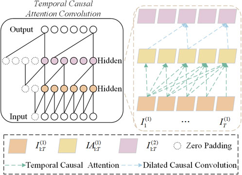
Figure 3. Temporal causal attention convolution, right-hand side, is illustrated using an example of five time steps, here, kernel size = 2 and dilation = 2.

2. Given ${\mathit{I}\mathit{A}}_{\mathbf{1}:\mathit{T}}^{\left(\mathit{L}\right)}$, we apply dilated causal convolution to it, as shown in Equation 7:

${\mathit{I}}_{\mathbf{1}:\mathit{T}}^{\left(\mathit{L}+\mathbf{1}\right)}=\mathit{D}\mathit{C}\mathit{C}\left({\mathit{I}\mathit{A}}_{\mathbf{1}:\mathit{T}}^{\left(\mathit{L}\right)}\right)(7)$

where ${\mathit{I}}_{\mathbf{1}:\mathit{T}}^{\left(\mathit{L}+\mathbf{1}\right)}$ represents the output of the dilated causal convolution, as illustrated in the top square on the right side of Figure 3. To maintain the output tensor’s length equal to the input tensor’s, zero padding of length $\left(\left(\mathit{k}-\mathbf{1}\right){\mathbf{2}}^{\mathit{l}-\mathbf{1}}\right)$ is added to the input tensor’s left side, as depicted in the Zero Padding on the left side of Figure 3, ensuring causal convolution.

3. The full temporal causal attention convolutional network is built by stacking L layers of temporal causal attention convolutions, covering both depth and time.

2.4.3 Temporal causal attention

Temporal causal attention, illustrated in Figure 4, involves integrating the influences of previous time steps into the current time step. Distinct from the self-attention structure, our attention mechanism selectively uses information from previous time steps only, thanks to a masking mechanism and optimized weight matrix, ensuring relevance to the current and preceding time steps while blocking future interactions.

Figure 4

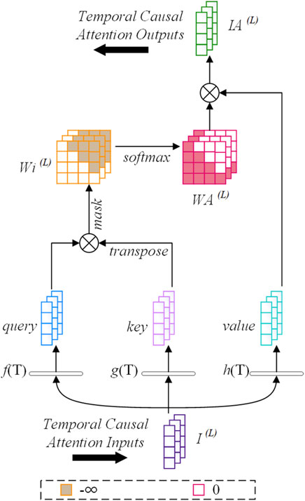
Figure 4. Illustration of the temporal causal attention mechanism, showing the integration of previous time steps’ influences into the current time step.

Initially, three linear transformations, f(T), g(T), and h(T), map ${\mathit{I}}_{\mathbf{1}:\mathit{T}}^{\left(\mathit{L}\right)}$ to ${\mathit{d}}_{\mathit{k}}$- dimensional $\mathit{q}\mathit{u}\mathit{e}\mathit{r}\mathit{i}\mathit{e}\mathit{s}\left({\mathit{q}}_{\mathbf{1}:\mathit{T}}^{\mathit{L}}=\mathit{f}\left({\mathit{I}}_{\mathbf{1}:\mathit{T}}^{\left(\mathit{L}\right)}\right)\right)$, $\mathit{k}\mathit{e}\mathit{y}\mathit{s}\left({\mathit{k}}_{\mathbf{1}:\mathit{T}}^{\mathit{L}}=\mathit{g}\left({\mathit{I}}_{\mathbf{1}:\mathit{T}}^{\left(\mathit{L}\right)}\right)\right)$, and ${\mathit{d}}_{\mathit{v}}$- dimensional $\mathit{v}\mathit{a}\mathit{l}\mathit{u}\mathit{e}\mathit{s}\left({\mathit{v}}_{\mathbf{1}:\mathit{T}}^{\mathit{L}}=\mathit{h}\left({\mathit{I}}_{\mathbf{1}:\mathit{T}}^{\left(\mathit{L}\right)}\right)\right)$. Subsequently, batch matrix multiplication calculates the dot products between ${\mathit{k}}_{\mathbf{1}:\mathit{T}}^{\mathit{L}}$ and ${\mathit{q}}_{\mathbf{1}:\mathit{T}}^{\mathit{L}}$, dividing each result by $\sqrt{{\mathit{d}}_{\mathit{k}}}$ to compute the weight matrix ${\mathit{W}\mathit{A}}^{\left(\mathit{L}\right)}$ , as shown in Equation 8:

${\mathit{W}}_{\mathit{i},\mathit{j}}^{\left(\mathit{L}\right)}=\frac{{\mathit{k}}_{\mathit{i}}^{\left(\mathit{L}\right)\mathit{T}}\cdot {\mathit{q}}_{\mathit{j}}^{\left(\mathit{L}\right)}}{\sqrt{{\mathit{d}}_{\mathit{k}}}}(8)$

Next, an upper triangular masking matrix ${\mathit{M}}^{\left(\mathit{L}\right)}$ is constructed, with elements on and below the diagonal set to 0, and those above the diagonal set to 1. The masking matrix ${\mathit{M}}^{\left(\mathit{L}\right)}$ is then applied to ${\mathit{W}}^{\left(\mathit{L}\right)}$ , as shown in Equation 9:

${\mathit{W}\mathit{i}}_{\mathit{i},\mathit{j}}^{\left(\mathit{L}\right)}=\left\{\begin{array}{c}{\mathit{W}}_{\mathit{i},\mathit{j}}^{\left(\mathit{L}\right)},\mathit{i}\mathit{f}{\mathit{M}}_{\mathit{i},\mathit{j}}^{\left(\mathit{L}\right)}=\mathbf{0}\\ -\mathit{\infty },\mathit{i}\mathit{f}{\mathit{M}}_{\mathit{i},\mathit{j}}^{\left(\mathit{L}\right)}=\mathbf{1}\end{array}\right.(9)$

For $\mathit{i},\mathit{j}=\mathbf{1},\mathbf{2},\cdots ,\mathit{T}$. Finally, a softmax function is applied to normalize ${\mathit{W}\mathit{i}}^{\left(\mathit{L}\right)}$ to obtain ${\mathit{W}\mathit{A}}^{\left(\mathit{L}\right)}$. This effectively suppresses the masked weights in ${\mathit{W}\mathit{i}}^{\left(\mathit{L}\right)}$ to nearly zero, thus isolating the future time step from the current one. Given ${\mathit{v}}_{\mathit{i}}^{\left(\mathit{L}\right)}$, the weighted output is calculated using the normalized weights, as shown in Equation 10:

$\mathit{I}{\mathit{A}}_{\mathit{t}}^{\left(\mathit{L}\right)}={\sum }_{\mathit{i}=\mathbf{0}}^{\mathit{t}}\mathit{W}{\mathit{A}}_{\mathit{i}}^{\left(\mathit{L}\right)}\cdot {\mathit{v}}_{\mathit{i}}^{\left(\mathit{L}\right)}(10)$

Here, ${\mathit{I}\mathit{A}}_{\mathit{t}}^{\left(\mathit{L}\right)}$ represents the output of the temporal attention, serving as the input for dilated causal convolution.

2.4.4 Dilated causal convolution

For a one-dimensional time series input $\mathit{x}\mathit{ϵ}{\mathit{R}}^{\mathit{n}}$ and a convolution kernel $\mathit{f}:\left\{\mathbf{0},\cdots ,\mathit{k}-\mathbf{1}\right\}\to \mathit{R}$, the dilated convolution operation F on an element s in the series is defined as shown in Equation 11:

$\mathit{F}\left(\mathit{s}\right)=\left(\mathit{x}{\ast }_{\mathit{d}}\mathit{f}\right)\left(\mathit{s}\right)={\sum }_{\mathit{i}=\mathbf{0}}^{\mathit{k}-\mathbf{1}}\mathit{f}\left(\mathit{i}\right)\cdot {\mathit{x}}_{\mathit{s}-\mathit{d}\cdot \mathit{k}}(11)$

Here, $\ast$ denotes the standard convolution operation, d the dilation factor, k the size of the convolution kernel, and $\mathit{s}-\mathit{d}\cdot \mathit{k}$ considers the elements in the past direction. When d = 1, the dilated convolution simplifies to a regular convolution. The dilated convolution expands the receptive field by increasing the size of the convolution kernel k and the dilation factor d. To encompass long-term historical data, the dilation factor follows an exponential growth strategy by setting d for layer i to ${\mathbf{2}}^{\mathit{i}}$.

Aligned with temporal causal attention, dilated causal convolution preserves causality in sequence prediction, preventing future time information from influencing the model. This causality is essential for the PM2.5 prediction task as it guarantees predictions are based solely on past and present data, excluding future information.

2.5 Experimental setup

The entire dataset is divided into three parts: training, validation, and test sets. The training set comprises the first 60% of each month’s data, while the validation set contains the last 20% of each month. Finally, the remaining 20% of data in each month is allocated to the test set. This division aims to preserve the time series continuity and adapt to monthly environmental changes, enhancing the model’s relevance to real-world scenarios. Our model forecasts 6-hour future predictions based on the past 24-hour readings, setting T = 24. To train our model, we employ the Adam optimizer, utilizing MSE as the loss function, with a batch size of 32. Through a grid search spanning the range {2, 3, 4, 5, 6, 7, 8} for the number of layers (levels) and kernel size in the temporal causal attention convolutional network, it was found that optimal performance is achieved with both parameters set to 4. For a more detailed analysis of these hyperparameters and their impact on model performance, please refer to Section 3.4. The model underwent 150 iterations, employing an early stopping strategy to prevent overfitting. Model performance evaluation employed three metrics: root mean square error (RMSE), mean absolute error (MAE), and the coefficient of determination (${\mathit{R}}^{\mathbf{2}}$) , as shown in Equations 12–14:

$\mathit{R}\mathit{M}\mathit{S}\mathit{E}=\sqrt{\frac{\mathbf{1}}{\mathit{n}}{\sum }_{\mathit{i}=\mathbf{1}}^{\mathit{n}}{\left({\mathit{y}}_{\mathit{i}}-{\widehat{\mathit{y}}}_{\mathit{i}}\right)}^{\mathbf{2}}}(12)$

$\mathit{M}\mathit{A}\mathit{E}=\frac{\mathbf{1}}{\mathit{n}}{\sum }_{\mathit{i}=\mathbf{1}}^{\mathit{n}}\mid {\mathit{y}}_{\mathit{i}}-{\widehat{\mathit{y}}}_{\mathit{i}}\mid (13)$

${\mathit{R}}^{\mathbf{2}}=\mathbf{1}-\frac{{\sum }_{\mathit{i}=\mathbf{1}}^{\mathit{n}}{\left({\mathit{y}}_{\mathit{i}}-{\widehat{\mathit{y}}}_{\mathit{i}}\right)}^{\mathbf{2}}}{{\sum }_{\mathit{i}=\mathbf{1}}^{\mathit{n}}{\left({\mathit{y}}_{\mathit{i}}-\overline{\mathit{y}}\right)}^{\mathbf{2}}}(14)$

Here, n is the total number of samples, ${\mathit{y}}_{\mathit{i}}$ the ith observed value, ${\widehat{\mathit{y}}}_{\mathit{i}}$ the ith predicted value, and $\overline{\mathit{y}}$ the average of observed values. Lower RMSE and MAE values signify higher prediction accuracy, while ${\mathit{R}}^{\mathbf{2}}$ ranges between 0 and 1, with values closer to 1 denoting a better model fit.

2.6 Experimental baseline model

Traditional time series prediction models like LSTM and GRU effectively address the issue of vanishing and exploding gradients in recurrent models through the use of gating mechanisms, showcasing robust performance in PM2.5 prediction tasks. These models were included in our comparative experiments.

CNN-BiLSTM (Du et al., 2021), among the earliest deep network models, adopts a joint spatio-temporal prediction approach by integrating CNN with BiLSTM.

ST-CausalConvNet (Zhang et al., 2021) highlights causality’s critical role in PM2.5 prediction, inspiring the development of our proposed temporal causal attention convolutional network.

TCAN (Hao et al., 2020), an exploratory feedforward sequence prediction network in NLP, combines convolution with an attention mechanism to approximate recurrent networks, laying the groundwork for our proposed temporal causal attention convolutional network. This model is included in a comparative experiment to underscore the significance of inter-site spatio-temporal feature extraction in multi-site PM2.5 prediction tasks.

DAGCGN (Tariq et al., 2023), developed in 2023 as a distance-adaptive graph convolutional gated recurrent network, excels in identifying complex spatio-temporal interactions between neighboring monitoring sites. Employing GCN in conjunction with the recurrent network GRU for multi-site PM2.5 prediction, this model demonstrates the recurrent model’s significant prediction performance and serves as our primary comparison model.

3 Results and discussion

3.1 Spatio-temporal correlation analysis result

We examined the default thresholds for spatio-temporal correlation analysis in the proposed model at four sample monitoring stations. Figure 5 shows the number of correlated stations identified at six different thresholds for sites numbered 1233, 1270, 1155, and 1141. Notably, these four sample sites are located in four distinct provinces within the dataset. As illustrated in Figure 5, we selected six specific thresholds—0.35, 0.40, 0.45, 0.50, 0.55, and 0.60—which are critical values between 0.35 and 0.60. At these thresholds, the number of correlated sites identified varies significantly, potentially impacting the model’s performance. Therefore, we focused on analyzing the effect of these thresholds on model accuracy. Additionally, we excluded thresholds below 0.35 and above 0.60 because they could either overly complicate or oversimplify the predictive model’s input feature vector, unlikely providing an optimal threshold. Specifically, thresholds below 0.35 might introduce a large number of sites with weak or no relevance to the target site, cluttering the model’s input feature vector with irrelevant features and reducing prediction accuracy. Conversely, thresholds above 0.60 could significantly reduce the number of correlated sites, potentially degrading the model to a single-site prediction and neglecting spatial correlation features between sites. We further investigated the optimal threshold among the selected values.

Figure 5

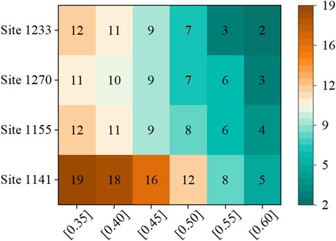
Figure 5. The number of relevant sites obtained at different thresholds for the four sample sites, with each row representing the number of relevant sites obtained at six different thresholds for that site.

Figure 6 shows the RMSE for the four sample sites when predictions are made using Causal-STAN at various thresholds. The results indicate a trend of decreasing and then increasing RMSE values for all four sites, with prediction error minimized at a threshold of 0.50. This suggests that thresholds set too high or too low adversely affect prediction outcomes: a high threshold limits spatially associated sites, losing key information, while a low threshold incorporates weakly related data, increasing noise and potential inaccuracies. Thus, a default threshold of 0.50 was adopted for Causal-STAN’s spatio-temporal correlation analysis in further model evaluations.

Figure 6

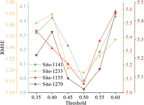
Figure 6. RMSE predicted for the four sample sites at different thresholds using Causal-STAN.

3.2 Model comparison results

To validate the effectiveness of our model, we conducted a performance evaluation using the test sets from all sites in the dataset. The final forecasting results for each model were determined by averaging the outcomes across 247 target sites. This approach helps to comprehensively assess the overall performance of each model across all sites, providing a thorough understanding of their predictive capabilities. Figure 7 displays a performance comparison between the proposed model and six competing models for forecasting the next 6 h, with results averaged over the 247 target sites. The results indicate that Causal-STAN outperforms the other models in predicting the next 6 h, achieving the lowest RMSE and MAE, along with the highest ${\mathit{R}}^{\mathbf{2}}$, whereas the classical GRU method exhibits the weakest performance. The performance among CNN-BiLSTM, ST-CausalConvNet, and DAGCGN is closely matched, with DAGCGN slightly leading; however, none surpass Causal-STAN.

Figure 7

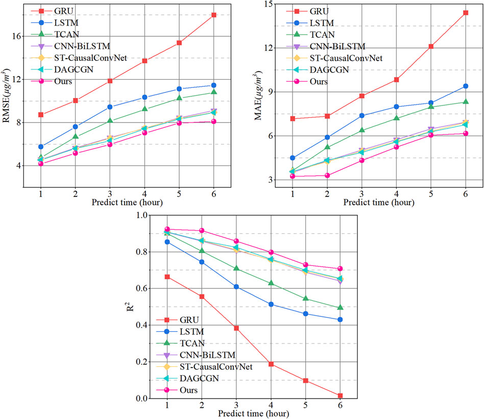
Figure 7. Comparison of the proposed Causal-STAN (Ours) with six other methods for hourly prediction, utilizing test data from all 247 stations.

Table 2 provides a comprehensive enumeration of the average results for the three evaluation metrics across each model, offering a thorough numerical comparison that complements the visual representation depicted in Figure 7. Experimental results indicate that TCAN significantly outperforms traditional time-series prediction models such as GRU and LSTM. This superior performance is largely attributed to TCAN’s unique model architecture. Unlike traditional recurrent prediction models based on RNN architecture, TCAN employs a TCN combined with an attention mechanism to predict PM2.5 concentrations. TCAN integrates the unique dilated convolutions of TCN with an attention mechanism, effectively expanding its receptive field in the time series and capturing long-term dependencies within the time series data. These features significantly enhance its performance in PM2.5 prediction tasks. However, a notable limitation of TCAN in multi-site PM2.5 prediction is its inability to perform spatial feature extraction. In contrast, CNN-BiLSTM surpasses TCAN by effectively capturing spatial dependencies between sites through CNN, yet it has its limitations. Although BiLSTM considers temporal features bi-directionally, this contradicts the causality principle of time series prediction. Additionally, the large parameter count and complex recurrent network structure of BiLSTM may impact model efficiency and performance. ST-CausalConvNet also utilizes CNN to capture spatial features but employs a feedforward network, TCN, for processing temporal features, ensuring that causality is integrated into the temporal prediction phase. This method effectively avoids future temporal information interference, giving ST-CausalConvNet a slight edge in predictive performance. This demonstrates that in PM2.5 prediction, feedforward predictive models and consideration of causality have distinct advantages. However, ST-CausalConvNet is limited in capturing long-distance dependencies in the time series and extracting internal correlation information from input data. In comparisons of predicting PM2.5 concentrations over the next 6 h, DAGCGN’s performance surpasses that of ST-CausalConvNet, thus exhibiting the best predictive performance among all baseline models. Unlike other baseline models, DAGCGN utilizes an enhanced GCN network combined with a GRU framework to effectively learn complex spatio-temporal features between sites. Yet, its limitation lies in the complex structure of the GCN network used during the spatial feature extraction phase. While this network adeptly captures spatial correlations between sites, it is restricted to processing a fixed number of related site features, allowing only a predefined number K of related sites per target site. Moreover, it is noteworthy that these baseline models do not account for the domain knowledge of air pollution dispersion or the directional characteristics of PM2.5 concentration dispersion between stations.

Table 2

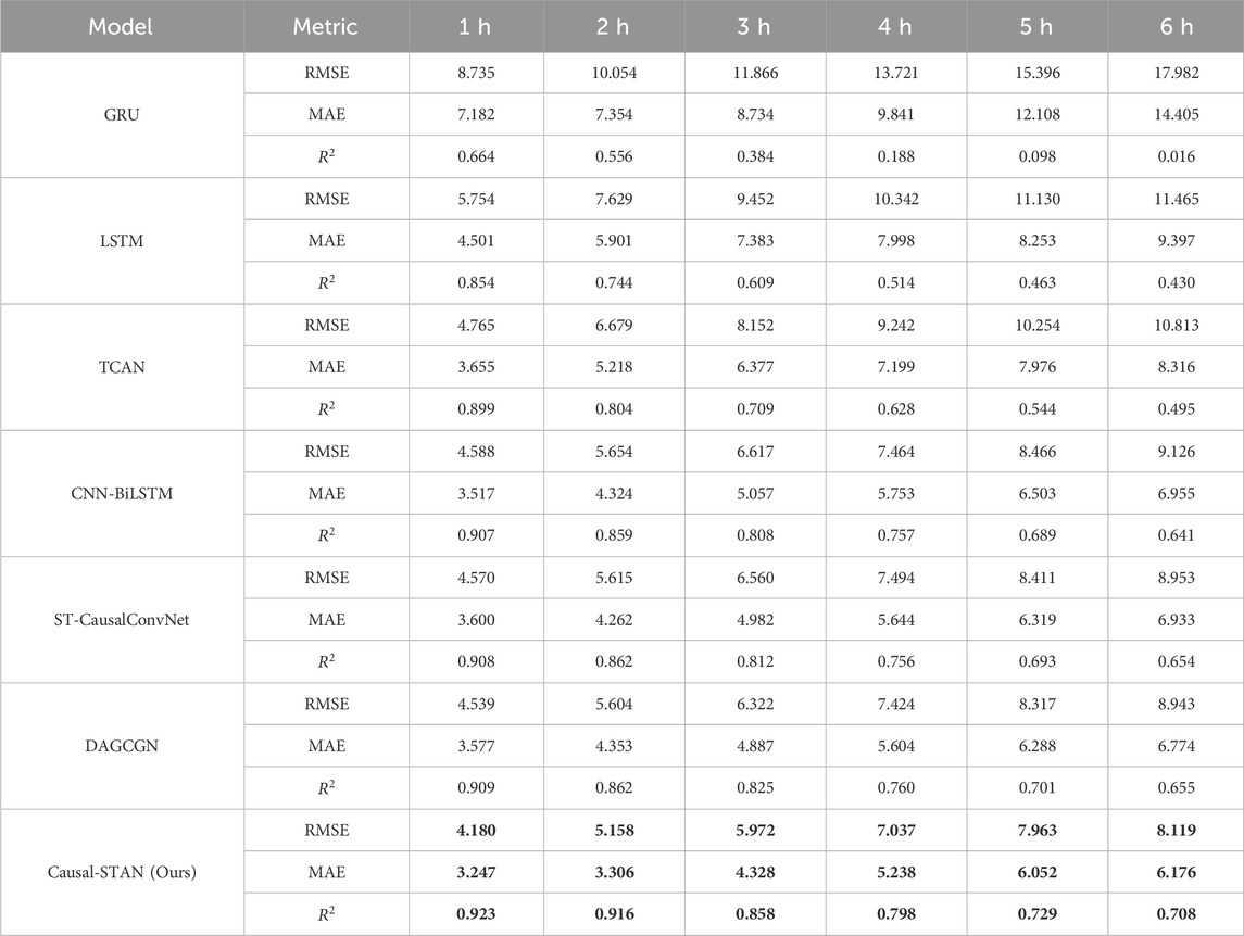
Table 2. Average metrics for each model based on test data from all 247 stations, with best results highlighted in bold.

Compared to DAGCGN, Causal-STAN reduces the RMSE by 7.91%, the MAE by 9.23%, and improves ${\mathit{R}}^{\mathbf{2}}$ by 1.54% for the next hour’s prediction. In the sixth-hour prediction, ${\mathit{R}}^{\mathbf{2}}$ for Causal-STAN remains at 0.708, still better than DAGCGN’s 0.655, with its RMSE and MAE also 9.21% and 8.82% lower, respectively. This outstanding performance is attributed to the unique architectural design of Causal-STAN. For spatial feature extraction, we employ CNNs to identify temporal local correlation trends and spatial correlations within the spatio-temporal data, and we introduce directional residual blocks to extract directional characteristics of PM2.5 concentration dispersion between sites. Compared to DAGCGN’s spatial feature extraction module, our module can conveniently handle model inputs with varying numbers of related sites. In terms of temporal feature processing, instead of using complex recurrent neural networks, we propose a more streamlined feedforward prediction network. By integrating TCN with an attention mechanism, we effectively capture the internal correlation information and long-term dependencies within the PM2.5 time series, providing an efficient alternative to recurrent network architectures.

To specifically showcase the predictive performance at a single target site, we selected site number 1141 and displayed its forecasting results on the test dataset, which consists of 1,749 data points, in a scatter plot format. Figure 8 presents the comparison of the linear correlation between the predicted and observed PM2.5 concentrations using our model, Causal-STAN, and six other models at this site. The results demonstrate that our model attains the highest correlation coefficient (${\mathit{R}}^{\mathbf{2}}=0.929$) and a better fit between the predicted regression line and the observed reference line.

Figure 8

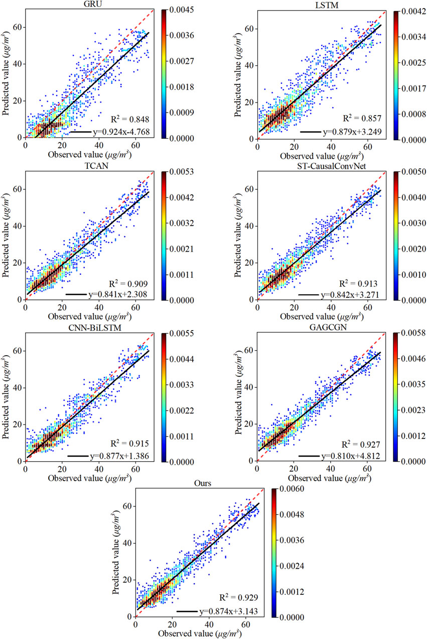
Figure 8. Correlation analysis between observed and predicted PM2.5 concentrations from various models on the test set at site number 1141. The dashed line is the y = x reference line and the solid line is the regression line.

3.3 Comparative evaluation of dataset partitioning strategies

To assess the effectiveness of our dataset partitioning strategy within the experimental framework, we conducted comparative experiments at four sample monitoring sites (IDs 1233, 1270, 1155, and 1141), contrasting our monthly partitioning approach (Causal-STAN) with the annual partitioning method commonly used in many models. Specifically, in the Causal-STAN method, the dataset is partitioned monthly with the first 60% designated for training, the subsequent 20% for validation, and the final 20% for testing. Conversely, in the comparative method (Causal-STAN-year), the dataset is divided annually, maintaining a consistent distribution of 60% for training, 20% for validation, and 20% for testing. This involves using data from the first 8 months of the year for training, data from September and October for validation, and the final 2 months’ data for testing. Throughout the experiment, both approaches were evaluated using the same model architecture, hyperparameters, and training settings.

Table 3 presents the forecasting results obtained at various test sites for both comparative methods. The Causal-STAN model consistently showed lower RMSE and MAE values across all sites, indicating a higher accuracy in predicting PM2.5 concentrations compared to the Causal-STAN-year model. For example, at site 1233, the RMSE for Causal-STAN was 3.189, compared to 3.758 for Causal-STAN-year, representing a 15.1% decrease. Similarly, the MAE decreased from 2.754 to 2.224, a reduction of about 19.2%. Furthermore, the ${\mathit{R}}^{\mathbf{2}}$ values, which measure the proportion of variance in the dependent variable that can be predicted from the independent variables, were also higher for Causal-STAN. Specifically, at site 1233, ${\mathit{R}}^{\mathbf{2}}$ improved from 0.928 with Causal-STAN-year to 0.951 with Causal-STAN, indicating a 2.5% increase in the model’s explanatory power and demonstrating a better fit to the observed data. At site 1155, the performance disparity was even more pronounced. The ${\mathit{R}}^{\mathbf{2}}$ value increased by 4.54%, underscoring the enhanced adaptability and predictive capacity of the monthly partitioning model under varied environmental conditions, which is crucial for accurate air quality forecasting.

Table 3

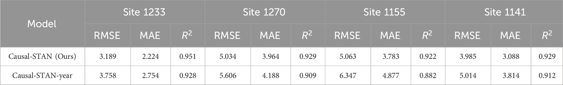
Table 3. Comparative performance analysis of causal-STAN and causal-STAN-year models at four monitoring sites.

The superior performance of the Causal-STAN model is primarily due to its ability to effectively capture short-term fluctuations and seasonal trends. The model’s monthly partitioning strategy ensures comprehensive inclusion of a wide array of critical environmental variables throughout the year during the training process. This granular approach provides the essential details necessary for accurately predicting changes in PM2.5 concentrations. Moreover, by integrating data from each month, the Causal-STAN model consistently represents the unique environmental characteristics and conditions of all seasons. This capability is particularly crucial for pollutants like PM2.5, which are highly sensitive to both seasonal variations and episodic changes. Consequently, this significantly enhances the model’s accuracy and robustness, enabling it to perform effectively across various times of the year. In contrast, the Causal-STAN-year model, while demonstrating reasonable performance during training and validation, exhibits a significant increase in error rates during the testing phase. This suggests an overfitting problem, where the model performs well on familiar data but struggles to adapt to new, unseen data. The annual partitioning contributes to this by smoothing over crucial short-term variations and anomalies within the dataset. Furthermore, this partitioning method may overlook critical PM2.5 variation patterns, such as lower concentrations in summer and higher in winter. Since the model is trained predominantly with summer data and tested on winter data, it fails to account for these seasonal trends. This explains why, despite effective training on large data blocks from the initial months, the model fails to accurately predict data from later months.

3.4 Hyperparameter study

In the temporal causal attention convolutional network, we investigated the effects of two crucial hyperparameters—number of layers (levels) and kernel size—on the Causal-STAN model using a grid search strategy. Experiments were performed at monitoring site number 1141. In this context, “levels” denotes the number of layers within the network architecture, reflecting the depth of the network, whereas “kernel size” indicates the dimension of filters within the network. Table 4 presents the performance of these parameters across various combinations, utilizing RMSE as the performance metric. The lowest RMSE (3.985) occurred when both parameters were set to 4, with minimal error variance around this configuration, highlighting that balanced selections of layers and kernel size are crucial for optimal performance.

Table 4

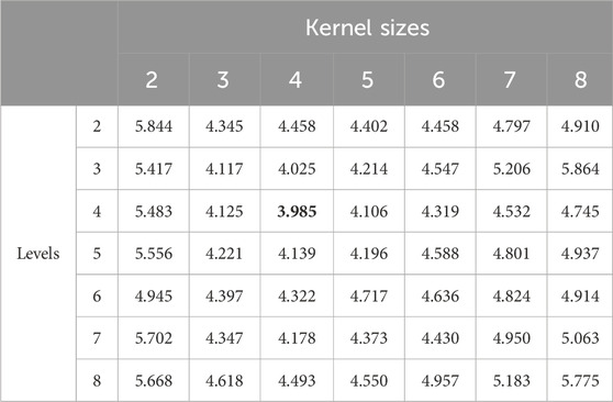
Table 4. Performance metrics of causal-STAN at various levels and kernel sizes using RMSE at monitoring site 1141, with best results highlighted in bold.

From the data in Table 4, it is evident that both overly large and small parameter values negatively affect model performance. For instance, when kernel sizes exceed 6 or levels surpass 6, RMSE increases noticeably, indicating overfitting or insufficient model generalization. Conversely, smaller values for these hyperparameters may lead to underfitting, as the network is unable to capture complex spatio-temporal relationships in the data.

The degradation in model accuracy stems from several factors. Too many layers increase the model’s complexity, which complicates optimization and risks overfitting. In contrast, an insufficient number of layers fails to capture deeper data relationships, leading to underfitting. Similarly, excessively large kernel sizes may include excessive historical information, introducing noise, while too small kernel sizes may not capture sufficient long-term dependencies.

As shown in Table 4, the optimal range for both levels and kernel size lies between 3 and 5. This range provides a balance between model complexity and generalization capability, ensuring more robust performance across different data conditions. These results highlight the importance of considering the combined effects of hyperparameters to maintain model accuracy.

4 Discussion

4.1 Effects of directional residual block

To validate the effectiveness of the directional residual block, two comparison strategies were employed: a) removing the directional residual block; b) substituting the directional residual block with a standard residual block (3 × 3 convolution). The outcomes, which reflect average data across all monitoring sites in the dataset, are presented in Figure 9. Initially, removing the directional residual block led to an increase in RMSE and MAE from 4.180 and 3.247 to 4.746 and 3.728, respectively, marking increases of 13.54% and 14.82%. Concurrently, ${\mathit{R}}^{\mathbf{2}}$ declined from 0.923 to 0.896, a decrease of 2.93%. This highlights the importance of incorporating domain knowledge in multi-site PM2.5 prediction. Conversely, incorporating standard residual blocks did not markedly enhance prediction performance. This indicates that the directional residual block effectively captures the directional characteristics of PM2.5 concentration diffusion between sites, and incorporating such domain knowledge is practically beneficial for PM2.5 prediction tasks.

Figure 9

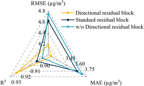
Figure 9. Impact of the directional residual block on prediction performance.

4.2 Effects of temporal causal attention

To evaluate the effectiveness of temporal causal attention for capturing temporal dependence, two comparison strategies were utilized: a) the removal of temporal causal attention, and b) the positioning of temporal causal attention after dilated causal convolution (DCC-TCA). The outcomes, which reflect average data across all monitoring sites in the dataset, are presented in Figure 10. Experimental results show a decrease in RMSE and MAE from 4.610 and 3.636 to 4.180 and 3.247, respectively, representing decreases of 9.33% and 10.70%, with ${\mathit{R}}^{\mathbf{2}}$ improving by 1.65% following the introduction of temporal causal attention. This underscores the importance of considering the time series’ long-term dependence.

Figure 10

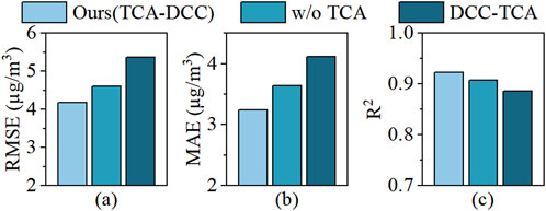
Figure 10. Impact of temporal causal attention on prediction performance: (A) RMSE, (B) MAE, and (C) R² comparisons for different models.

Positioning temporal causal attention after dilated causal convolution significantly diminishes the model’s predictive performance. Compared to the proposed temporal causal attention convolutional network, there is a significant increase in RMSE and MAE, and a notable decrease in ${\mathit{R}}^{\mathbf{2}}$ by 4.01%. This phenomenon could be attributed to dilated causal convolution losing or weakening critical temporal information during computation, hindering temporal causal attention from fully compensating for this loss. Hence, this confirms the superiority of our proposed temporal causal attention convolutional network design.

5 Conclusion

This study introduces Causal-STAN, a novel spatio-temporal attention causal convolutional neural network, tailored for multi-site PM2.5 prediction. It addresses prevalent issues in existing methods, such as over-reliance on recurrent networks for temporal dependency extraction, limited exploration of feedforward modeling, and neglect of air quality pollutant dispersion domain knowledge. Causal-STAN integrates a multi-site spatio-temporal feature integration module and a temporal causal attention convolutional network, significantly enhancing spatial and temporal dependency learning while introducing causality into temporal dependency analysis. Combining a convolutional neural network with a directional residual block, Causal-STAN effectively captures directional features of PM2.5 dispersion and utilizes dilated causal convolution and attention mechanisms as viable alternatives to recurrent networks for long-term dependency learning. Research results indicate that Causal-STAN can accurately forecast PM2.5 concentrations across multiple monitoring station areas for the next 6 hours, outperforming current methodologies. Specifically, its application in forecasting future PM2.5 concentrations for 247 air quality monitoring stations in the Yangtze River Delta region of China will significantly assist policymakers in more effectively evaluating and addressing air quality issues. This enhancement in predictive capability is crucial for improving public health protection and mitigating health risks associated with air pollution.

Despite the encouraging results, the Causal-STAN model has several limitations. So far, the model has only been applied to the prediction of PM2.5, and its generalizability to other pollutants, such as NO₂ or O₃, remains uncertain. Additionally, the model has only been tested in the Yangtze River Delta region, and its performance in areas with different climatic or environmental conditions has yet to be validated. The model also relies on data from existing air quality monitoring stations, which limits its effectiveness in regions with scarce monitoring infrastructure. Furthermore, data gaps are currently filled using traditional interpolation techniques, which may not fully capture the complexity of missing data. Finally, external factors such as industrial emissions or policy changes, which may occur unexpectedly, have not yet been considered, and these factors could potentially affect the model’s predictive performance.

In the future, we plan to enhance our model along three targeted dimensions:

(1) Data Completion Using Deep Learning: We will integrate advanced deep learning methods, such as generative adversarial networks (GANs) or autoencoders, to perform more accurate data imputation. Preliminary experiments using a small subset of incomplete data suggest that these techniques can significantly improve the model’s performance in regions with data gaps. We expect that adopting these methods will enhance overall predictive accuracy, especially in areas where air quality monitoring stations have significant data missing for certain periods.

(2) Geographical Expansion: We plan to obtain extensive pollutant data and air quality indices from the past year for the Jing-Jin-Ji or Pearl River Delta regions through the urban air quality real-time publishing platform of the China National Environmental Monitoring Center, as well as corresponding meteorological data from the National Climatic Data Center. Using data from these regions, we aim to validate the model’s predictive performance under different climatic and environmental conditions. These results will guide us in refining the model for better generalization and applicability across diverse geographical areas.

(3) Application in Unmonitored Areas: We plan to collect additional data sources for unmonitored areas through open-source APIs, including functional area classification, road network data, weather forecast data, and pollutant and meteorological data from the nearest air quality monitoring stations. Furthermore, we will improve the model’s training strategy with a focus on simulating the interactions between different monitoring stations. By leveraging these enriched data sources, we aim to predict pollutant levels in unmonitored areas, addressing a critical gap in air quality management and providing stronger support for public health initiatives.

Data availability statement

The original contributions presented in the study are included in the article/supplementary material, further inquiries can be directed to the corresponding author.

Author contributions

YW: Funding acquisition, Methodology, Project administration, Resources, Supervision, Writing–review and editing. ST: Conceptualization, Data curation, Investigation, Methodology, Software, Visualization, Writing–original draft. PZ: Conceptualization, Formal Analysis, Validation, Writing–review and editing.

Funding

The author(s) declare that no financial support was received for the research, authorship, and/or publication of this article.

Acknowledgments

We thank the faculty and staff of the School of Computer Science and Technology for their support and assistance in providing the necessary resources and environment to conduct our research.

Conflict of interest

The authors declare that the research was conducted in the absence of any commercial or financial relationships that could be construed as a potential conflict of interest.

Publisher’s note

All claims expressed in this article are solely those of the authors and do not necessarily represent those of their affiliated organizations, or those of the publisher, the editors and the reviewers. Any product that may be evaluated in this article, or claim that may be made by its manufacturer, is not guaranteed or endorsed by the publisher.

Footnotes

¹https://air.cnemc.cn:18007/

²https://www.ncei.noaa.gov/

References

Ai, S., Wang, C., Qian, Z., Cui, Y., Liu, Y., Acharya, B. K., et al. (2019). Hourly associations between ambient air pollution and emergency ambulance calls in one central Chinese city: implications for hourly air quality standards. Sci. Total Environ. 696, 133956. doi:10.1016/j.scitotenv.2019.133956

PubMed Abstract | CrossRef Full Text | Google Scholar

Bi, J., Zhang, X., Yuan, H., Zhang, J., and Zhou, M. (2022). A hybrid prediction method for realistic network traffic with temporal convolutional network and LSTM. IEEE Trans. Automation Sci. Eng. 19, 1869–1879. doi:10.1109/TASE.2021.3077537

CrossRef Full Text | Google Scholar

Chen, M.-H., Chen, Y.-C., Chou, T.-Y., and Ning, F.-S. (2023). PM2.5 concentration prediction model: a CNN–rf ensemble framework. Int. J. Environ. Res. Public Health 20, 4077. doi:10.3390/ijerph20054077

PubMed Abstract | CrossRef Full Text | Google Scholar

Chiang, P.-W., and Horng, S.-J. (2021). Hybrid time-series framework for daily-based PM _2.5 forecasting. IEEE Access 9, 104162–104176. doi:10.1109/ACCESS.2021.3099111

CrossRef Full Text | Google Scholar

Chinatamby, P., and Jewaratnam, J. (2023). A performance comparison study on PM2.5 prediction at industrial areas using different training algorithms of feedforward-backpropagation neural network (FBNN). Chemosphere 317, 137788. doi:10.1016/j.chemosphere.2023.137788

PubMed Abstract | CrossRef Full Text | Google Scholar

de Hoogh, K., Héritier, H., Stafoggia, M., Künzli, N., and Kloog, I. (2018). Modelling daily PM2.5 concentrations at high spatio-temporal resolution across Switzerland. Environ. Pollut. 233, 1147–1154. doi:10.1016/j.envpol.2017.10.025

PubMed Abstract | CrossRef Full Text | Google Scholar

Du, S., Li, T., Yang, Y., and Horng, S.-J. (2021). Deep air quality forecasting using hybrid deep learning framework. IEEE Trans. Knowl. Data Eng. 33, 2412–2424. doi:10.1109/TKDE.2019.2954510

CrossRef Full Text | Google Scholar

Erden, C. (2023). Genetic algorithm-based hyperparameter optimization of deep learning models for PM2.5 time-series prediction. Int. J. Environ. Sci. Technol. 20, 2959–2982. doi:10.1007/s13762-023-04763-6

CrossRef Full Text | Google Scholar

Faraji, M., Nadi, S., Ghaffarpasand, O., Homayoni, S., and Downey, K. (2022). An integrated 3D CNN-GRU deep learning method for short-term prediction of PM2.5 concentration in urban environment. Sci. Total Environ. 834, 155324. doi:10.1016/j.scitotenv.2022.155324

PubMed Abstract | CrossRef Full Text | Google Scholar

Gao, X., Huang, J., Cardenas, A., Zhao, Y., Sun, Y., Wang, J., et al. (2022). Short-term exposure of PM _2.5 and epigenetic aging: a quasi-experimental study. Environ. Sci. Technol. 56, 14690–14700. doi:10.1021/acs.est.2c05534

PubMed Abstract | CrossRef Full Text | Google Scholar

Grell, G. A., Peckham, S. E., Schmitz, R., McKeen, S. A., Frost, G., Skamarock, W. C., et al. (2005). Fully coupled “online” chemistry within the WRF model. Atmos. Environ. 39, 6957–6975. doi:10.1016/j.atmosenv.2005.04.027

CrossRef Full Text | Google Scholar

Hao, H., Wang, Y., Xue, S., Xia, Y., Zhao, J., and Shen, F. (2020). Temporal convolutional attention-based network for sequence modeling. arXiv Prepr. arXiv:2002.12530. doi:10.48550/arXiv.2002.12530

CrossRef Full Text | Google Scholar

Khandelwal, U., He, H., Qi, P., and Jurafsky, D. (2018). “Sharp nearby, fuzzy far away: how neural language models use context,” in Proceedings of the 56th annual meeting of the association for computational linguistics (volume 1: long papers) (Stroudsburg, PA, USA: Association for Computational Linguistics), 284–294. doi:10.18653/v1/P18-1027

CrossRef Full Text | Google Scholar

Lagesse, B., Wang, S., Larson, T. V., and Kim, A. A. (2020). Predicting PM _2.5 in well-mixed indoor air for a large office building using regression and artificial neural network models. Environ. Sci. Technol. 54, 15320–15328. doi:10.1021/acs.est.0c02549

PubMed Abstract | CrossRef Full Text | Google Scholar

Lai, X., Li, H., and Pan, Y. (2021). A combined model based on feature selection and support vector machine for PM2.5 prediction. J. Intelligent and Fuzzy Syst. 40, 10099–10113. doi:10.3233/JIFS-202812

CrossRef Full Text | Google Scholar

Li, W., Wei, Y., An, D., Jiao, Y., and Wei, Q. (2022). LSTM-TCN: dissolved oxygen prediction in aquaculture, based on combined model of long short-term memory network and temporal convolutional network. Environ. Sci. Pollut. Res. 29, 39545–39556. doi:10.1007/s11356-022-18914-8

PubMed Abstract | CrossRef Full Text | Google Scholar

Liang, J., and Tang, W. (2022). Ultra-short-term spatiotemporal forecasting of renewable resources: an attention temporal convolutional network-based approach. IEEE Trans. Smart Grid 13, 3798–3812. doi:10.1109/TSG.2022.3175451

CrossRef Full Text | Google Scholar

Liang, Y., Xia, Y., Ke, S., Wang, Y., Wen, Q., Zhang, J., et al. (2023). AirFormer: predicting nationwide air quality in China with transformers. Proc. AAAI Conf. Artif. Intell. 37, 14329–14337. doi:10.1609/aaai.v37i12.26676

CrossRef Full Text | Google Scholar

Liu, B., Tan, X., Jin, Y., Yu, W., and Li, C. (2021). Application of RR-XGBoost combined model in data calibration of micro air quality detector. Sci. Rep. 11, 15662. doi:10.1038/s41598-021-95027-1

PubMed Abstract | CrossRef Full Text | Google Scholar

Liu, H., and Chen, C. (2020). Prediction of outdoor PM2.5 concentrations based on a three-stage hybrid neural network model. Atmos. Pollut. Res. 11, 469–481. doi:10.1016/j.apr.2019.11.019

CrossRef Full Text | Google Scholar

Liu, Z., Jiang, P., De Bock, K. W., Wang, J., Zhang, L., and Niu, X. (2024). Extreme gradient boosting trees with efficient Bayesian optimization for profit-driven customer churn prediction. Technol. Forecast Soc. Change 198, 122945. doi:10.1016/j.techfore.2023.122945

CrossRef Full Text | Google Scholar

Marsha, A., and Larkin, N. K. (2019). A statistical model for predicting PM _2.5 for the western United States. J. Air Waste Manage Assoc. 69, 1215–1229. doi:10.1080/10962247.2019.1640808

PubMed Abstract | CrossRef Full Text | Google Scholar

Marvin, D., Nespoli, L., Strepparava, D., and Medici, V. (2022). A data-driven approach to forecasting ground-level ozone concentration. Int. J. Forecast 38, 970–987. doi:10.1016/j.ijforecast.2021.07.008

CrossRef Full Text | Google Scholar

Nasr Azadani, M., and Boukerche, A. (2022). A novel multimodal vehicle path prediction method based on temporal convolutional networks. IEEE Trans. Intelligent Transp. Syst. 23, 25384–25395. doi:10.1109/TITS.2022.3151263

CrossRef Full Text | Google Scholar

Reshef, D. N., Reshef, Y. A., Finucane, H. K., Grossman, S. R., McVean, G., Turnbaugh, P. J., et al. (2011). Detecting novel associations in large data sets. Science 334, 1518–1524. doi:10.1126/science.1205438

PubMed Abstract | CrossRef Full Text | Google Scholar

Shakya, D., Deshpande, V., Goyal, M. K., and Agarwal, M. (2023). PM2.5 air pollution prediction through deep learning using meteorological, vehicular, and emission data: a case study of New Delhi, India. J. Clean. Prod. 427, 139278. doi:10.1016/j.jclepro.2023.139278

CrossRef Full Text | Google Scholar

Sun, Y., Ding, J., Liu, Z., and Wang, J. (2023). Combined forecasting tool for renewable energy management in sustainable supply chains. Comput. Ind. Eng. 179, 109237. doi:10.1016/j.cie.2023.109237

CrossRef Full Text | Google Scholar

Tariq, S., Tariq, S., Kim, S., Woo, S. S., and Yoo, C. (2023). Distance adaptive graph convolutional gated network-based smart air quality monitoring and health risk prediction in sensor-devoid urban areas. Sustain Cities Soc. 91, 104445. doi:10.1016/j.scs.2023.104445

CrossRef Full Text | Google Scholar

Teng, M., Li, S., Yang, J., Wang, S., Fan, C., Ding, Y., et al. (2023). Long-term PM2.5 concentration prediction based on improved empirical mode decomposition and deep neural network combined with noise reduction auto-encoder- A case study in Beijing. J. Clean. Prod. 428, 139449. doi:10.1016/j.jclepro.2023.139449

CrossRef Full Text | Google Scholar

Vaswani, A., Shazeer, N., Parmar, N., Uszkoreit, J., Jones, L., Gomez, A. N., et al. (2017). Attention is all you need. arXiv Prepr. arXiv:1706.03762. doi:10.48550/arXiv.1706.03762

CrossRef Full Text | Google Scholar

Wang, H., Zhang, L., Wu, R., and Cen, Y. (2023). Spatio-temporal fusion of meteorological factors for multi-site PM2.5 prediction: a deep learning and time-variant graph approach. Environ. Res. 239, 117286. doi:10.1016/j.envres.2023.117286

PubMed Abstract | CrossRef Full Text | Google Scholar

Wang, J., Wang, D., Zhang, F., Yoo, C., and Liu, H. (2024a). Soft sensor for predicting indoor PM2.5 concentration in subway with adaptive boosting deep learning model. J. Hazard Mater 465, 133074. doi:10.1016/j.jhazmat.2023.133074

PubMed Abstract | CrossRef Full Text | Google Scholar

Wang, J., Wu, T., Mao, J., and Chen, H. (2024b). A forecasting framework on fusion of spatiotemporal features for multi-station PM2.5. Expert Syst. Appl. 238, 121951. doi:10.1016/j.eswa.2023.121951

CrossRef Full Text | Google Scholar

Wang, P., Zhang, H., Qin, Z., and Zhang, G. (2017). A novel hybrid-Garch model based on ARIMA and SVM for PM 2.5 concentrations forecasting. Atmos. Pollut. Res. 8, 850–860. doi:10.1016/j.apr.2017.01.003

CrossRef Full Text | Google Scholar

Wang, S., Li, Y., Zhang, J., Meng, Q., Meng, L., and Gao, F. (2020). “PM2.5-GNN,” in Proceedings of the 28th international conference on advances in geographic information systems (New York, NY, USA: ACM), 163–166. doi:10.1145/3397536.3422208

CrossRef Full Text | Google Scholar

Wu, E. M.-Y., and Kuo, S.-L. (2012). Air quality time series based GARCH model analyses of air quality information for a total quantity control district. Aerosol Air Qual. Res. 12, 331–343. doi:10.4209/aaqr.2012.03.0051

CrossRef Full Text | Google Scholar

Yan, R.-H., Peng, X., Lin, W., He, L.-Y., Wei, F.-H., Tang, M.-X., et al. (2022). Trends and challenges regarding the source-specific health risk of PM _2.5 -bound metals in a Chinese megacity from 2014 to 2020. Environ. Sci. Technol. 56, 6996–7005. doi:10.1021/acs.est.1c06948

PubMed Abstract | CrossRef Full Text | Google Scholar

Yang, Z., Mahendran, R., Yu, P., Xu, R., Yu, W., Godellawattage, S., et al. (2022). Health effects of long-term exposure to ambient PM2.5 in asia-pacific: a systematic review of cohort studies. Curr. Environ. Health Rep. 9, 130–151. doi:10.1007/s40572-022-00344-w

PubMed Abstract | CrossRef Full Text | Google Scholar

Young, T., Hazarika, D., Poria, S., and Cambria, E. (2018). Recent trends in deep learning based natural language processing [review article]. IEEE Comput. Intell. Mag. 13, 55–75. doi:10.1109/MCI.2018.2840738

CrossRef Full Text | Google Scholar

Zhang, B., Zou, G., Qin, D., Ni, Q., Mao, H., and Li, M. (2022). RCL-Learning: ResNet and convolutional long short-term memory-based spatiotemporal air pollutant concentration prediction model. Expert Syst. Appl. 207, 118017. doi:10.1016/j.eswa.2022.118017

CrossRef Full Text | Google Scholar

Zhang, L., Na, J., Zhu, J., Shi, Z., Zou, C., and Yang, L. (2021). Spatiotemporal causal convolutional network for forecasting hourly PM2.5 concentrations in Beijing, China. Comput. Geosci. 155, 104869. doi:10.1016/j.cageo.2021.104869

CrossRef Full Text | Google Scholar

Zhou, H., Zhang, F., Du, Z., and Liu, R. (2021). Forecasting PM2.5 using hybrid graph convolution-based model considering dynamic wind-field to offer the benefit of spatial interpretability. Environ. Pollut. 273, 116473. doi:10.1016/j.envpol.2021.116473

PubMed Abstract | CrossRef Full Text | Google Scholar

Zhu, J., Deng, F., Zhao, J., and Zheng, H. (2021). Attention-based parallel networks (APNet) for PM2.5 spatiotemporal prediction. Sci. Total Environ. 769, 145082. doi:10.1016/j.scitotenv.2021.145082

PubMed Abstract | CrossRef Full Text | Google Scholar