 Tim J. Arciszewski
 Erin. J. Ussery
 Gerald R. Tetreault
 Keegan A. Hicks3
 Mark E. McMaster
94% of researchers rate our articles as excellent or good
Learn more about the work of our research integrity team to safeguard the quality of each article we publish.
Find out more
ORIGINAL RESEARCH article
Front. Environ. Sci., 18 July 2024
Sec. Toxicology, Pollution and the Environment
Volume 12 - 2024 | https://doi.org/10.3389/fenvs.2024.1405357
This article is part of the Research TopicModeling for Environmental Pollution and ChangeView all 6 articles
Industrial development in Canada’s oil sands region influences the ambient environment. Some of these influences, such as the atmospheric deposition of emitted particles and gases are well-established using chemical indicators, but the effects of this process on bioindicators examined in field studies are less well-supported. This study used an extensive dataset available from 1997 to 2019, spatio-temporal modeling (Integrated Nested Laplace Approximation), and data on industrial and non-industrial covariates, including deposition patterns estimated using HYSPLIT (Hybrid Single Particle Lagrangian Integrated Trajectory) to determine if changes in sentinel fishes collected in streams from Canada’s Oil Sands Region were associated with oil sands industrial activity. While accounting for background variables (e.g., precipitation), estimated deposition of particles emitted from mine fleets (e.g., Aurora North), in situ stacks (e.g., Primrose and Cold Lake), mine stacks (e.g., Kearl), mine dust (e.g., Horizon), road dust (e.g., Muskeg River mine), land disturbance in hydrologically-connected areas, and wildfires were all associated with at least one fish endpoint. While many individual industrial stressors were identified, a specific example in this analysis parallels other work: the potential influence of emissions from both Suncor’s powerhouse and dust emitted from Suncor’s petroleum coke pile may both negatively affect fish health. Comparisons of fitted values from models with the estimated industrial effects and with deposition rates set to zero suggested some negative (and persistent) influences of atmospheric deposition at some locations, such as the gonadosomatic index (GSI) in the lower Muskeg and Steepbank rivers. While there is evidence of some large differences at individual locations the mean GSI and body condition estimates have improved throughout the region since the beginning of these collections in the late 1990s potentially highlighting improved environmental performance at the facilities, widespread enrichment effects, or interactions of stressors. However, mean liver-somatic indices have also slightly increased but remain low. These results, coupled with others suggest the utility of spatio-temporal approaches to detect the influence and effects of oil sands development at both local and regional scales.
The environmental performance of the facilities used to extract and process bitumen occurs in Canada’s Oil Sands Region (OSR) has been heavily scrutinized for decades. In response to this scrutiny, many monitoring programs measuring multiple indicators in various media have been used to determine how these clustered operations influence the environment (Roberts et al., 2022b). While the findings from the work varies, some of the clearest results of residual effects in the ambient environment have been found in studies of contaminants of concern (CoCs), such as metals and organics measured in natural archives, including peat and lake sediments (e.g., Kurek et al., 2013; Shotyk et al., 2017). These results demonstrate multiple spatial and temporal patterns, but they typically suggest greater concentrations of CoCs in the environment close to facilities and increasing in time after the construction of the first mine. These results have also been corroborated by repeated spatial surveys of other indicators, such as lichens and snow (e.g., Gopalapillai et al., 2019; Landis et al., 2019). While other information is also available, such as the declining deposition of metals in snow over time (Gopalapillai et al., 2019), collectively the results of the studies using natural archives and repeated surveys highlight the primary role of area, fugitive, and stack emissions from oil sands facilities and the subsequent atmospheric deposition of particles on the concentration of CoCs in ambient environment (Arciszewski et al., 2022a; Roberts et al., 2022a; Horb et al., 2022).
While many studies from the OSR highlight the effect of atmospheric deposition on chemical indicators measured in various media (e.g., Horb et al., 2022), some gaps remain, including its potential influence on flowing waters. Studies done in depositional areas of streams over multiple years have found inconsistent evidence of impacts from any industrial development (Evans et al., 2016) suggesting some or much of the deposited material is retained in landscape features, such as wetlands (Shotyk et al., 2017; Landis et al., 2019; Wasiuta et al., 2019; Wieder et al., 2022). If the deposited materials do migrate to streams, other work suggests the mobilized particulates are accompanied by eroded and weathered bitumen and minerals naturally present in streams (Birks et al., 2017; Droppo et al., 2018). Separating the influence of natural and anthropogenic stressors in flowing waters has been and remains a persistent challenge for identifying the effects of industrial activity in the OSR (Culp et al., 2021).
Similar to the discrepancies in chemical indicators, the responses of biota to industrial stressors have also not been consistent across studies. Studies in lakes have also suggested little evidence of biological effects from atmospheric deposition (Hazewinkel et al., 2008; Parsons et al., 2010; Kurek et al., 2013; Summers et al., 2016), while work in the Athabasca River suggests the exposure to naturally-derived substances drives changes in benthic invertebrates (Gerner et al., 2017). Studies also suggest the substances present in snow collected within 7 km of the industrial sites are toxic to larval fish, but these effects disappear when fish are exposed to the stream water collected during the spring thaw (Parrott et al., 2018). Other analyses of resident fish also suggest few discernible differences have occurred over space or time near industrial facilities (Tetreault et al., 2003b; 2020) supporting the results from the laboratory exposures (Parrott et al., 2018). In contrast, other work has suggested effects of atmospheric deposition may be present in some indicators. For example, some indices derived from the intensity of production at each facility were correlated with fish health metrics of lake chub (Couesius plumbeus) captured in the Ells River (Arciszewski et al., 2022b). These results, along with others from benthic invertebrates (Arciszewski, 2021) and water quality (Arciszewski and Roberts, 2022) suggest associations with particles deposited and eventually washed into streams. Other results from spawning fish (Schwalb et al., 2015), mosses (Wieder et al., 2016), amphibians (Mundy et al., 2019), and birds (Fernie et al., 2018) also suggest impacts from atmospherically-deposited substances may be occurring in biota.
These potential effects in biota across media coupled with some potential challenges with comparing chemical data from multiple studies (Birks et al., 2017) and with the timing of sample collection (Parrott et al., 2018) further suggest that effects of atmospheric deposition on stream biota cannot be ruled out. However, existing studies typically use short-term collections and spatial reference sites (or temporal reference periods) to determine if oil sands industrial activity may be affecting biota residing in streams (Tetreault et al., 2003b; Arciszewski et al., 2022b). Similarly, no studies have yet directly compared the deposition of particles to the landscape and the responses of biological indicators in flowing waters, such as fish. The purpose of this study was to assemble a data set from existing records available from the OSR to examine this gap following the data-discovery paradigm (Hey et al., 2009). The biotic indicator chosen for this work is the sentinel fish. Between 1997 and 2019, thousands of fish were collected across multiple tributaries for multiple programs (RAMP, 1999; Tetreault et al., 2020; Arciszewski et al., 2022b; Wynia et al., 2022). Importantly, the period of these collections, although samples are missing from some years and no data are available prior to any industrial development, also coincides with substantial changes in the oil sands industry; between 1997 and 2019, 7 of the 9 operating mines were constructed and opened and all but 2 of the in-situ facilities (Imperial Cold Lake and Canadian Natural Peace River) began production culminating in a 6.5-fold increase in total production from all facilities (Oil Sands Magazine, 2024). The size of the dataset combined with its spatial and temporal coverage are valuable assets needed to examine the effects of the coinciding oil sands industrial activities.
While the fish records are substantive and cover a period of industry expansion, there are some challenges with examining historical data, such as a lack of natural and anthropogenic stressor information. For example, while more detailed studies of deposition began after ∼ 2012 (e.g., Harner et al., 2018), these data are not available for earlier field surveys of aquatic indicators (e.g., RAMP, 1999). The historical atmospheric deposition can, however, be estimated using atmospheric trajectory and dispersion models, such as the Hybrid Single-Particle Lagrangian Integrated Trajectory model (HYSPLIT; Stein et al., 2015). HYSPLIT has been evaluated and used for multiple studies (e.g., Sunderland et al., 2008; Moroz et al., 2010; Chen et al., 2013; Schade and Gregg, 2022), including some in the OSR (e.g., Cho et al., 2014; Blanchard et al., 2021). Similar to other models, HYSPLIT can be used for both point source emissions, such as Suncor’s powerhouse and Mildred Lake’s flue-gas desulpherizer, stacks from steam generators, and for wind-blown dusts (Draxler et al., 2010). However, the model can also run on desktop computers using its open-access software and the modelling scenarios can be scripted using R (Iannone, 2016). While other models can also be used (e.g., Bullock and Brehme, 2002; Makar et al., 2018), this combination of attributes makes HYSPLIT a suitable candidate for estimating atmospheric deposition in the OSR.
Reconstructing deposition patterns across the landscape is necessary to harness the historical fish dataset and determine the potential effects of this elusive effect pathway on biota. For example, estimating the effects of atmospheric deposition can allow the calculation of expected ranges of fish measurements in its absence or other scenario modelling, but the analyses of fish data in the OSR requires two additions. First, other factors, such as local climate and land disturbance may also influence the health of fish (Arciszewski et al., 2022b). Wildfires also occur commonly in the region, including large fires in 2011 and 2016 (Government of Alberta, 2024b) and can affect water quality (Emmerton et al., 2020). Fortunately, data describing these events are readily available and can also be integrated into the analysis to better account for additional sources of variation and highlight the potential influence of industrial stressors. Second, techniques which can account for the spatio-temporal relationships of the data are needed. Recent advances in statistical modelling, such as the Integrated Nested Laplace Approximation implementation in R (R-INLA) can be used to identify unmeasured covariates, account for spatial and/or temporal auto-correlation among the measurements, and include other random effects, including multiple species (Rue et al., 2009; Lindgren et al., 2011).
The modelled deposition data in combination with the assembled fish dataset, additional stressor information, and spatio-temporal modelling provides a novel opportunity to gain deeper insights into the effects of industrial activities in Canada’s OSR. The general purpose of this broad and novel analysis was to provide initial information on the potential effects of atmospheric deposition on small-bodied fishes residing in the OSR, to better understand the current constraints of monitoring in the region, and how new approaches may benefit the existing studies. More specifically, these general goals were translated into three main questions: 1) are any of the industrial predictors associated with metrics of fish health for small-bodied fish sampled lethally? 2) how do these estimates change with the addition of fish sampled during the non-lethal and fish assemblage programs? and 3), what are the relative differences in fish metrics calculated from models with and without the estimated deposition rates?
Given the amount and variety of pre-work required to examine these data (e.g., amalgamation of fish data, deposition modelling, acquiring additional stressor data, watershed delineation), a summary of the methods are provided here, but detailed descriptions are provided in the Supplementary Material.
The primary focus of the current analysis was to describe the variation in fish measurements of body mass, liver mass, and gonad mass obtained from lethal “tributary” programs in the OSR (e.g., Tetreault et al., 2003b; 2020; Arciszewski et al., 2022b). The implementation of INLA in R (R-INLA) was used to account for random spatial and temporal effects and for various attributes of the measurements, including sex (male and female) and species, covariates, including other fish measurements (e.g., length for body mass (BM) and BM for liver mass (LM) and gonad mass (GM)), background climate variables, wild fire area, and industrial factors, including land disturbance and estimated atmospheric deposition. While informative, these primary analyses were also augmented with secondary analyses on BM using fish collected following the non-lethal EEM protocols (2004–2009; e.g., RAMP, 2009) and protocols developed for fish assemblage monitoring (FAM) in the OSR (e.g., 2009–2019; RAMP, 2009; Wynia et al., 2022).
The available fish data was collected across multiple, but related iterations of studies done since the late 1990s. The analysis here focused on individual measurements of small-bodied sentinel species repeatedly sampled in tributary sites: lake chub, longnose dace (Rhinichthys cataractae), and slimy sculpin (Cottus cognatus). From the initiation of sampling following guidance for the Environmental Effects Monitoring (EEM) approach developed for other sectors, but applied to the OSR, fish have been collected at 40 stream reaches across 8 tributaries to the Athabasca River (Calumet, Tar, Ells, MacKay, Horse, Steepbank, Muskeg, Firebag rivers), 3 to the Clearwater River (High Hills, Christina, Hangingstone rivers) and 1 to the Birch River (Alice Creek; Figure 1; Supplementary Tables S1–S9). While sample sizes vary by sex, year, and reach combination (1–40), the total sample sizes of individual adult fish used for the analyses of lethal BM, LM, and GM are 4,020, 3,502, and 3,562, respectively.
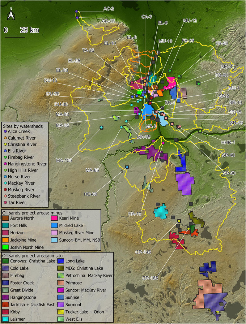
Figure 1. Fishing locations for lethal sampling (coloured circles), oil sands project areas in various stages of operation, and topography (high to low is brown to green) in regional study area; CNRL Peace River (not shown) is roughly 280 km west of the HO-80 site; divides for watersheds sampled in lethal programs and additional watersheds included in non-lethal programs shown in yellow and orange, respectively; Fort McMurray shown in black; additional sampling locations included in FAM program shown as dark grey squares; site names for FAM locations shown in Supplemental Figure S1.
As mentioned above, additional data on fish measurements are also available for the OSR (Supplementary Figure S1). These two additional fish monitoring programs were non-lethal collections (e.g., Gray et al., 2002) used by RAMP from 2004–2009 and the Fish Assemblage Monitoring (FAM) begun in RAMP in 2009 (RAMP, 2010) and continued in the current program (Wynia et al., 2022). The total sample size of BM with the non-lethal and lethal EEM samples is 5,910. When these EEM data are combined with the all of the FAM species data, the sample size for body masses is 10,380. An additional analysis using FAM data only for the lethally-sampled species (lake chub, longnose dace, and slimy sculpin) was also done to better understand if and how the data from the two programs (EEM and FAM) could be combined into a single analysis. The sample size for this analysis is 8,952. These secondary datasets are referred to as All-EEM, EEM + FAM, and EEM + FAM3, respectively.
HYSPLIT was used to estimate the deposition location of particles emitted from point, mobile, and area sources in the OSR. Particle sources included stacks, wind-blown dust (mine brownfields and petroleum coke piles), mechanically-generated road dust, and mine fleet exhaust. Particles deposited in hydrologically isolated areas were removed. The North American Regional Reanalysis climate dataset was used for modelling (Supplementary Figure S2). A qualitative comparison between summertime deposition in 2015 estimated from HYSPLIT and observed in bogs (Mullan-Boudreau et al., 2017) was also done and indicated generally agreement between the observed and modeled deposition (Supplementary Figure S3). The outputs from the deposition modelling are not fully presented in either the main text or in the Supplementary Material. However, some figures are provided in the latter (i.e., Supplementary Figures S4–S7) and the deposition patterns expected from Suncor’s powerhouse (Figure 2) generated from the raw deposition data and Kernel Density Estimation (cell size = 10 km2, bandwidth = 25 km) using the hotspot_kde function in the sfhotspot R package (Ashby, 2023) show the spatial and temporal variation on the concentration of particulates and reflect patterns interpolated or suggested in other studies (e.g., Kurek et al., 2013; Kirk et al., 2014; Jautzy et al., 2015).
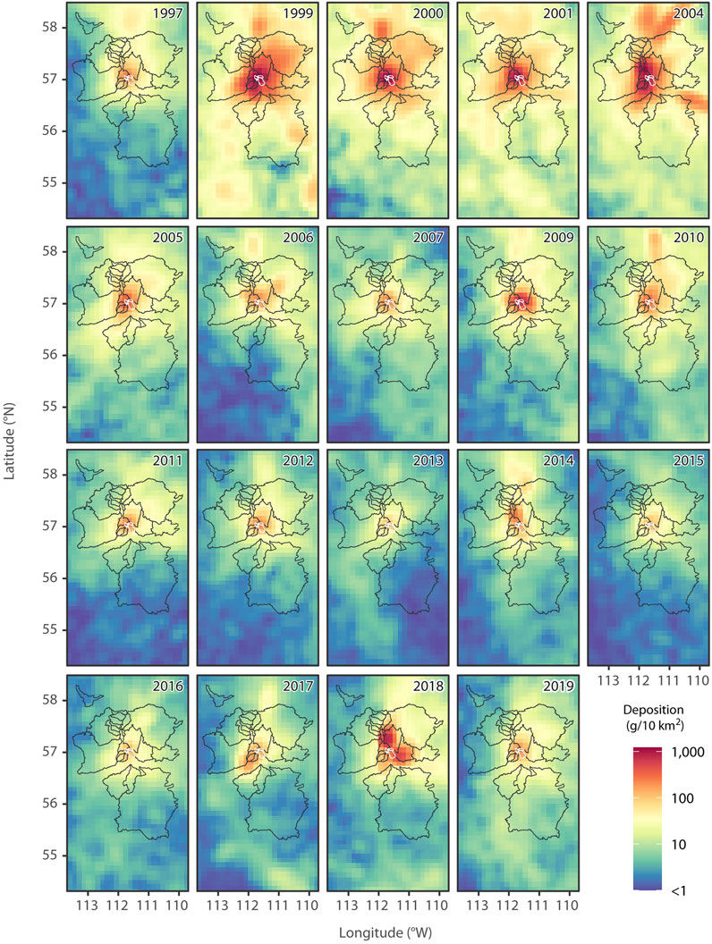
Figure 2. Deposition of particulates (g/10 km2) from Suncor’s powerhouse stack estimated using HYSPLIT and Kernel Density Estimation; black outlines show watersheds of all tributaries sampled in both lethal and non-lethal fish programs; white outline shows the extent of Suncor’s mining project area (basemine, Millenium mine, and North Steepbank).
Other data needed to perform this analysis were required. These additional data included upstream (e.g., upslope, pour point) areas for each unique fish sampling coordinate (Government of Alberta, 2024a), proportion of land disturbance outside of the hydrologically isolated areas (Alberta Biodiversity Monitoring Institute, 2024), wildfire area (Government of Alberta, 2024b), and modelled estimates of air temperature (mean air temperature was estimated as the mid-point between the available minima and maxima), precipitation, and sunlight intensity (Government of Alberta, 2024a) were obtained.
The primary fish analyses done here used the lethally-sampled (adult) fish and were done on GM, LM, and BM using Gaussian distributions. All industrial variables (deposition and land disturbance), climate/other variables (e.g., air temperature and wildfire area), fish variables (sex, species, sex by species interactions, and fish size covariates (BM for LM and GW and total or fork length for BM)) were initially included. Terms for the collection type (lethal vs. non-lethal) and the study type (EEM vs. FAM) were also included in the secondary BM analyses. Fish measurements were transformed following initial analyses and examination of residual plots. Box-Cox transformations were used to normalize the fish data. All numerical covariates were scaled and centered to N (0,1).
While many approaches can be used (e.g., Santos-Fernandez et al., 2022), INLA and its implementation in R (INLA-R Rue et al., 2014) met the needs of this analysis. INLA is a widely applicable and available Bayesian technique which can be used in place of the Markov Chain Monte Carlo to estimate posterior probabilities for latent Gaussian models traditionally examined using a general linear models (Rue et al., 2009). The versatile INLA can also be used to understand non-linear patterns in data, used to fit generalized additive models, and can easily incorporate spatial, temporal, and/or spatio-temporal effects, including spatial data collected over unequal temporal intervals (Lindgren et al., 2011; Zuur et al., 2017; Krainski et al., 2018).
Previous work has suggested variables such as discharge and Julian Day of sample collection can influence metrics of fish health (Arciszewski et al., 2022b). However, not all variables relevant for modelling fish health in the OSR are available for all samples. While additional modelling could be used to reconstruct some of these data, random temporal and spatial effects were used to account for its absence. Additionally, three spatio-temporal effects were evaluated. These included no spatio-temporal effect, a replicated (temporally independent spatial field) and an auto-regressive (AR1) spatio-temporal effect. The auto-regressive (order 1) spatial fields were estimated using 1-year knots in a 1-D mesh to account for the unequal sampling intervals between the sampling events; for example, no lethal measurements of GM and LM occurred in the OSR between 2001 and 2010. The potential spatial random variation associated with collecting multiple fish from the same site and the proximity of sampling locations to each other was modelled using the stochastic partial differential equation (SPDE) approach to solve the Matérn Covariance Function available in INLA (Lindgren et al., 2011). A spatial 2D mesh was derived from a simplified stream network polygon and used a cutoff of 500 m using constrained refined Delaunay triangulation (Supplementary Figure S8). The analyses followed examples provided in Blangiardo and Cameletti (2015), Zuur et al. (2017), Krainski et al. (2018), and Moraga (2020).
Substantial multi-collinearity among the industrial predictors was identified using variance inflation factors (VIF) and variable clustering (as per Harrell, 2015). Rather than initially pool, combine, remove, or otherwise decompose the individual sources to overcome the multi-collinearity, weakly informative priors were used to reduce overfitting of the fixed effects (Gelman et al., 2013). Use of priors is also advocated to reduce or control spatial confounding effects (Zimmerman and Ver Hoef, 2022). For the non-industrial predictors and for the proportion of burned area, the default Gaussian priors used in INLA (N (0, 31.622)) were used. In contrast, more skeptical and regularizing priors were used for the deposition estimates (Gelman et al., 2013; McElreath, 2018). These more skeptical priors for the industrial variables were set at N (0, 3.1622).
Initial analyses for each fish measurement endpoint were done using two sets of covariates. First, “base” models with only fish-related (e.g., sex, species) or study design covariates (e.g., non-lethal or lethal sampling) were evaluated. Next, these base models were augmented with all industrial and climatic covariates and these full models were also evaluated. Additionally, each of the full and base models for each set of fish data were run using no, a replicated, or an auto-correlated spatio-temporal field. The best model for each fish measurement was identified using the Deviance Information Criterion (DIC). Among these results, the replicated spatio-temporal fields were often either the best or among the best explanatory models; replicated spatio-temporal field also run much faster than their auto-correlated counterparts. Given these two features, the replicated spatio-temporal fields were used for further modelling.
The further analyses included forward selection for models in which the base models were identified as the best (i.e., LM and EEM + FAM BM) and backwards elimination for those in which the full models were identified by DIC. Backwards elimination also included the removal of covariates to create a more parsimonious model using a DIC threshold of 2.
The importance of the predictors in the final models was determined following the credibility interval criterion (Van Erp et al., 2019) and using 95% coverage. Using this criterion, a variable is considered more important when the 95% credibility interval does not include zero and considered less important when it does. The analysis focused on interpreting the climate, wildfire, industrial, and spatio-temporal effects and the marginal posterior distributions for covariates associated with fish, such as sex and species are provided in the Supplementary Information (Supplementary Figure S9).
While the information from marginal posterior distributions of the final covariates of each fish measurement analysis is informative, the final models for lethally-sampled fish were used to back-transform the results into terms relevant to the fish health literature. First, relative percent differences between “exposed” (with estimated deposition) and “reference” (with estimated deposition set to zero) scenarios were calculated. These fitted values from both scenarios were first used to calculate expected fish health endpoints, body condition (k), liver-somatic index (LSI), and gonadosomatic index (GSI) for each individual fish. Secondly, the percent differences of the results from the exposure scenario relative to reference scenario were calculated. These percent differences were compared to the ranges of critical effect sizes (CES) used for these fish metrics (Munkittrick et al., 2009). Changes of the percent differences over time (i.e., slopes) for each fish measurement over time were calculated using a linear regression. The CESs were also highlighted in four focal watersheds: Ells, MacKay, Steepbank, and Muskeg rivers. These calculations were also performed for the secondary analyses of body mass.
Expected ranges of fish measurements used in EEM-like surveys, GSI, LSI, and k in the absence of atmospheric deposition were also estimated from lethally sampled fish. The GSI, LSI, and k values for fish estimated from the “reference” scenario were also calculated and presented as potential ranges of expected variation (central 95% prediction intervals). These data are provided in the Supplementary Material.
Several assumptions about atmospheric deposition were made during this analysis. A constant association between particulates emitted from each individual source and their chemical properties, including contaminants of concern was assumed. The total mass of particles deposited to each fish site watershed was likely an underestimate of the true value, but we also assumed the masses (between the actual and the estimated) are proportional. Furthermore, we also assumed the estimated mass of deposited particles was proportional to the mass of particles reaching streams during direct or indirect deposition.
The primary set of analyses included only the lethally sampled fishes and for each endpoint, six models were initially assessed (Table 1). Among the lethal analyses, the best fitting models included both the set of industrial and climate/other variables and the replicated spatial fields (Table 1), but the analyses of LM and lethal BM also suggested the AR (1) models performed similarly. Among the analyses of these lethal EEM endpoints, the DICs indicated full models performed better than the base models for GM and BM, but the opposite was true for LM. Additionally, while including non-industrial and industrial covariates improved the models without spatio-temporal fields, none of these models were identified as the best or were within 2 units of the minimum DIC in most cases, the improvements of the models by including the random spatio-temporal terms was marked (Table 1). These patterns were typically reflected in the RMSEs.
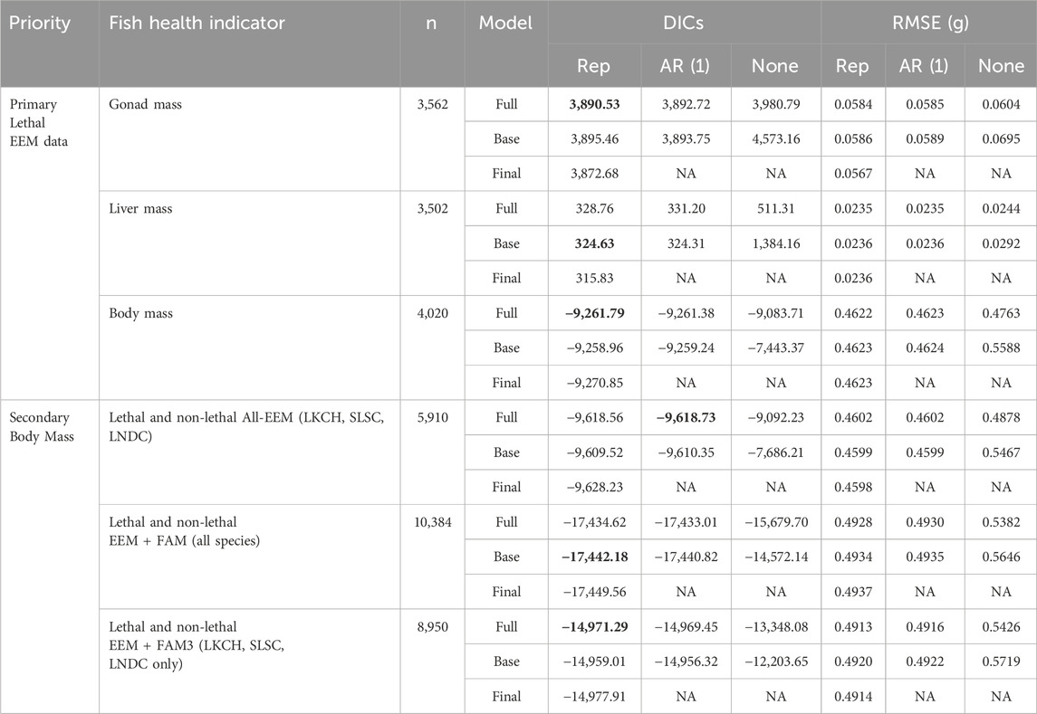
Table 1. Deviance Information Criterion (DIC) and the root mean squared error (RMSE) for Integrated Nested Laplace Approximation (INLA) models of fish health indicators with and without random spatio-temporal random effects (replicated (Rep.), AR (1), no spatio-temporal effects (none), industrial predictors, or climate variables; within model types, bolded values are the lowest DICs within a fish health indicator category among the full and base models; LKCH = lake chub; SLSC = slimy sculpin; LNDC = longnose dace; NA = Not Applicable.
The secondary analyses of the BM data using the available non-lethal data also indicated the improvement in model performance when using a replicated spatio-temporal field. The only analysis suggesting the AR (1) field out-performed the replicated field was the analysis using the All-EEM BM data, but this improvement was small (Table 1). The secondary analyses of BM data also indicated the full models better explained the responses in the All-EEM and the EEM + FAM3 analysis. In contrast, the EEM + FAM analyses (using all species) suggested the base model performed the best.
Backwards elimination was used to improve the parsimony of the full models: GM, lethal BM, All-EEM, and EEM + FAM3. In contrast, forward addition was used for LM and the EEM + FAM using all species. Among the lethal analyses, the stepwise procedures included 36, 17, and 37 industrial and non-industrial variables for GM, LM, and BM, respectively (Figure 3). In contrast, fewer variables were retained in the All-EEM and EEM + FAM analyses (12 and 4 respectively; Figure 3), but 53 were retained in the EEM + FAM3 analyses. Only two variables, Mildred Lake mine fleet and Fort Hills mine fleet were not identified by the stepwise procedure for any fish measurement. Among the lethal analyses the Mildred Lake flue gas desulpherizer (FGD), Horizon stacks, mine dust at Mildred Lake and Jackpine, road dust from Kearl, mine fleets at Suncor Basemine, Mildred Lake, and Fort Hills, and petcoke dust from Mildred Lake were not included in final models. Among the secondary BM models, stack emissions from Suncor MacKay River, Imperial Cold Lake, CNRL Primrose, and Athabasca Hangingstone, mine dust from Aurora North and North Steepbank, road dust from Aurora North, emissions from the Mildred Lake and Fort Hills mine fleets, and wildfire area were not included in the final models.
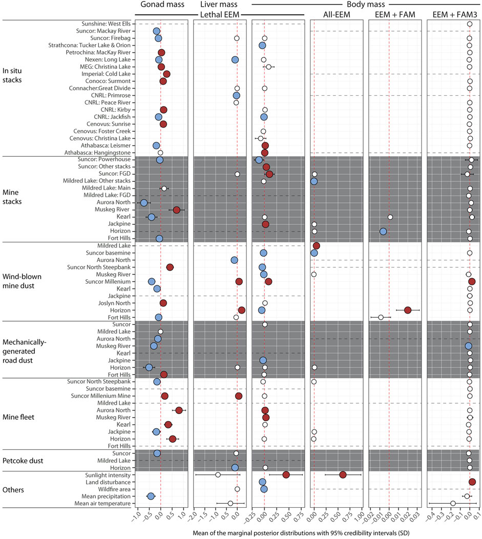
Figure 3. Mean marginal posterior distributions and 95% credibility intervals of standardized (0,1) variables; red and blue shaded symbols respectively show variables with more important positive and negative effects; open symbols denote variables included in the final models but considered less important; horizontal dashed lines show variables not identified across subsets of fish endpoints (e.g., all analyses, primary lethal, or secondary BM; FGD = flue gas desulpherizer; project areas locations shown in Figure 1.
The spatio-temporal effects were estimated for measurements of BM, LM, and GM of fishes residing in the OSR. The ranges (θ) estimated from the Matérn covariance functions are roughly 2,100, 7,600, and 4,900 m for the analyses of GM, LM, and lethal BM, respectively (Supplemental Figure S10). Among the secondary BM analyses, the ranges extended from roughly 7,000 m in the All-EEM dataset, but shrank to ∼870 m in the two BM analyses using the FAM and EEM data (Supplemental Figure S10). The estimated random spatio-temporal effects for GM, LM, and lethal BM ranged from −0.240 to 0.301, −0.386 to 0.381, and −0.061 to 0.090 g, respectively (Supplemental Figures S11–S16). Among the secondary BM analyses, the spatio-temporal random effects were larger than indicated in the primary BM analyses. The estimated spatio-temporal effects for the secondary BM analyses ranged from −0.318 to 0.156, −0.292 to 0.220, and −0.263 to 0.241 g, for the respective All-EEM, EEM + FAM, and EEM + FAM3 datasets (Supplemental Figures S11–S16) indicating more spatio-temporal variation in these spatially (and temporally) expanded analyses.
While simultaneously accounting for spatial and temporal variation, the 95% credibility intervals of the marginal posterior distributions for most of the industrial covariates describing the deposition patterns and retained by the stepwise procedures did not overlap with zero and were deemed important (Figure 3).
Clear and overall patterns by types of particle sources were not obvious, but some general signals were apparent among the lethal analyses (Figure 3). Positive associations between mine fleet emissions, such as Aurora North and Millenium with GM, LM, and lethal BM responses were common, but negative associations (e.g., North Steepbank with GM) or less important associations (e.g., North Steepbank with BM) were also identified (Figure 3). Road dust variables also showed either negative or less important associations with the lethal fish endpoints (Figure 3). Across the lethal fish endpoints, eight of thirteen more important associations of mine dust were negative, but only one of three was negative among the LM estimates (Figure 3). Among the in situ stacks, eleven were either positively (six) or negatively (five) associated with GM; the estimated emissions and deposition of particles from in situ stacks were also evenly split in BM (two each) and in LM only two were deemed more important than others (Figure 3); in this case, both more important variables were negatively associated with LM.
Among the secondary BM analyses, few industrial variables were included. Among those included variables, few were also deemed more important than others (Figure 3). More specifically, potentially important effects from stack emissions at Suncor identified in the primary BM analysis were either not included or downgraded in the secondary analyses using data from more years and more. However, many less important variables were identified in the EEM + FAM3 analyses. For example, all but six in situ and mining stacks had less important effects on BM of fishes included in the EEM + FAM3 analyses. However, potentially important negative effects were identified across all of the secondary BM analyses, including Mildred Lake’s miscellaneous “other” stacks, Horizon stacks, Suncor Basemine dust, and road dust from the Muskeg River mine. Across these secondary BM analyses, more important positive associations were identified in mine dust from Mildred Lake, Millenium, and Horizon.
More detailed information can also be gleaned from the marginal posterior distributions. Among the lethal analyses, delayed petcoke dust emitted from Suncor and Horizon were selected and deemed more important in the GM and LM models, respectively, but fluid coke dust from Mildred Lake was not identified in any of the lethal models; all three were identified, but as less important in the EEM + FAM3 BM analyses (Figure 3). Similarly, the three stack sources modelled for Suncor (the FGD, powerhouse, and amalgamated miscellaneous (e.g., other) stacks) were all identified as more important variables in the lethal BM model; the powerhouse emissions were also associated with negative effects in GM, while the FGD at Suncor were associated with less important effects in LM. In contrast, Mildred Lake’s FGD was not selected in a lethal fish model while the main and “other” stacks at Mildred Lake were associated with less important effects in GM and lethal BM, respectively. The contrast in the results from the stacks at Suncor and Mildred Lake (as well as Horizon, the only other mine in the region with a coker) suggests an important feature of operations at Suncor may be driving some changes in fish health indicators at some sites.
Relative land disturbance in hydrologically-connected areas of watersheds was not associated with important effects on LM and GM, but was associated with lower BM (Figure 3). However, greater land disturbance was associated with positive effects in the EEM + FAM3 analyses. Among the climate variables, sunlight intensity had a positive effect in the lethal BM analyses (which was also identified in the All-EEM analyses) along with a less important negative effect on LM (Figure 3). Mean precipitation was associated with a more important negative influence on GM and with a less important effect on BM in the EEM + FAM3 analysis (Figure 3). In contrast, the estimated mean air temperature was only identified as having a less important and negative effect on LM and the EEM + FAM3 fishes (Figure 3).
While the effects of individual emissions and subsequent deposition of particles may be instructive and many may be important, their collective effects are also relevant and, in some cases, may be substantial. Over time and for all lethally sampled fishes, the conditional means of the percent differences of GSI, LSI, and k increased between 1997 and 2019 (Figure 4); the slopes of these changes are 2%, 0.115%, and 0.311% per year for GSI, LSI, and k, respectively. A general pattern of increasing GSI, LSI, and k is also true for some watersheds and specific reaches. For example, both GSI and k of fish collected at the SR-1 site has increased over time (Figure 4). However, there is also
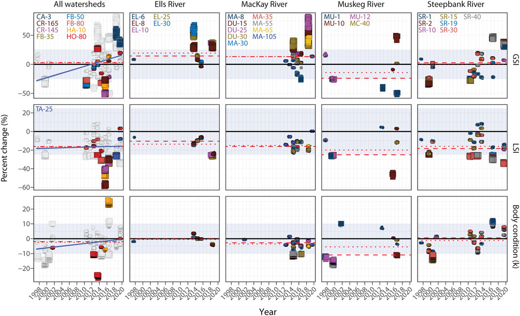
Figure 4. Expected change in fish health indices with atmospheric deposition compared to removing these effects for all captured fish across all sites (all watersheds) or specific focal watersheds (Ells, MacKay, Muskeg, and Steepbank rivers); blue shading shows generic CESs used in other studies of fish health; circles show fish within the expected range (0 ± CES); squares indicate potential differences larger than CES; means and medians for measurement and watersheds shown by horizontal dotted and dashed lines, respectively; differences for all non-focal watersheds shown in Supplemental Figure 17.
Some data suggesting declines at individual locations may also be occurring monotonically or sporadically over time, including LSI at the SR-30 (e.g., 2010–2012, 2016, 2019) and SR-40 (2012, 2016) sites (Figure 4). Another example of a localized decline within a broader regional increase is GSI in fish captured at the MU-1 site in the lower Muskeg River. The GSI of fish captured at this site has been progressively lower than expected over time (Figure 4). The lower Muskeg site MU-1, although it has not been ignored in sampling events, has, however, not been intensively sampled over time compared to other sites, such as the SR-1 site in the lower Steepbank and the patterns at the MU-1 site are challenging to interpret with certainty. Similar challenges for site-specific interpretations are also apparent in other estimated changes, including those observed in the MacKay River in 2018.
Some large changes in the relative differences of fish health metrics with and without the industrial effects are also predicted (Figure 4). Large declines in GSI, including some which are between 60% and 80% are predicted in many of the non-focal watersheds, such as the Christina. Large declines in GSI are also predicted at sites in the Firebag, Hangingstone, MacKay, Muskeg, and Steepbank. More specifically, in the Steepbank River, both the SR-15 and SR-2 sites sampled in 1999 had lower GSI than expected (Figure 4). The two sites sampled in the Muskeg River in 1999, MU-1 and MU-12, also both showed large declines in GSI (Figure 4). However, large increases in GSI are also predicted for some watersheds, including the Calumet, Horse, Ells, MacKay, Muskeg, and multiple sites sampled in the Steepbank (Figure 4). While no large increases in LSI are predicted, declines of roughly 60% in LSI in fish exposed to atmospheric deposition are predicted from the model applications, including fish captured at the CR-165 site. Large declines in LSI may also be present in the Tar, Horse, Firebag, Ells, Muskeg, and Steepbank Rivers. Similar to GSI, large declines at both locations sampled in each of the Muskeg and Steepbank Rivers in 1999 were observed in LSI.
The maximum percent differences from 0 in lethal BM are of a similar magnitude compared to GM and LM (roughly 2.5 times the standard CES; Figure 4). The largest differences in k estimated for lethally-sampled fish are predicted for the Horse, MacKay, Muskeg, and Steepbank Rivers. Similar to the GSI and LSI estimates for fish collected before in the Muskeg and Steepbank Rivers, declines in k exceeding the standard CES of −10% were observed at both the upstream and downstream sites in sampling done before 2002 (Figure 4).
Among the secondary analyses of BM, the predicted magnitude of effects of industrial variables are typically smaller when compared to the primary lethal analyses, but occasional large differences were identified. Among these analyses large declines may be apparent in fish captured at the Fort Creek location (FO-2) along with sites in the Muskeg River; Figure 5). Increases exceeding the CES may also have occurred in the Calumet, Muskeg, and Steepbank Rivers (Figure 5). While the maximum magnitude of the predicted differences were smaller in the secondary BM analyses, the temporal changes in mean conditional k were also smaller. The slopes of the changes over time for the All-EEM and EEM + FAM3 analyses were 0.242 and 0.167 %, respectively (Figure 5). While also a smaller magnitude, the slope for the changes in the EEM + FAM analyses was also negative (−0.021).
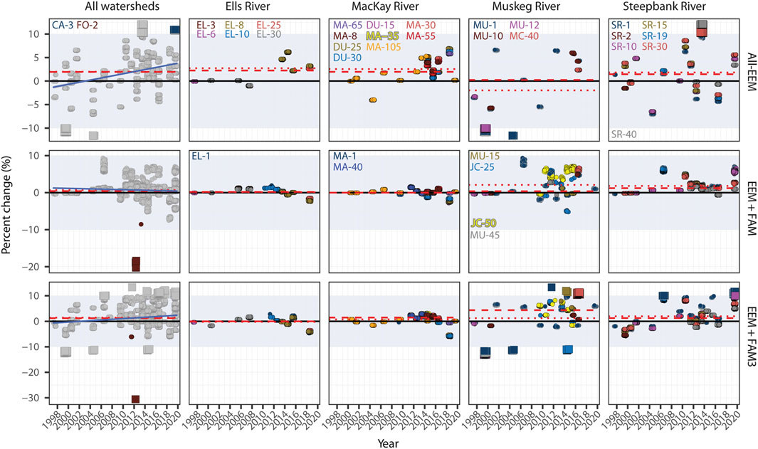
Figure 5. Estimated differences in fish health endpoints with and without the estimated effects of atmospheric deposition for the secondary body mass analyses across all sites (all watersheds) or specific focal watersheds (Ells, MacKay, Muskeg, and Steepbank rivers) sampled in the Oil Sands Region between 1997 and 2019; blue shading shows generic CESs (±10%) used in other studies of fish health; circles show fish within the expected range; squares indicate potential differences outside expected range; horizontal dotted line shows median of differences for measurement and watershed; horizontal dashed line shows mean of differences for measurement and watershed.
To better understand the potential role of industrial variables driving changes at particular sites over time, or at multiple sites over time, some example variables were identified and their potential influence on fish residing at particular locations is explored here. For example, stack emissions from the CNRL Kirby facility are positively associated with changes in GM (Figure 3). The highest rates of deposition of particles emitted from this facility from this facility occur in the Christina basin (Figure 6). Similarly, the deposition of particles emitted from Suncor’s powerhouse were predicted to predominantly occur in the Steepbank and Muskeg Rivers. Other localized patterns of deposition occur in particles emitted from Aurora North’s mine fleet (Figure 6). Other sources show a much more uniform and widespread distribution, such as petcoke dust from Suncor, whereas others, such as Imperial Cold Lake and Nexen Long Lake show patterns both consistent with local deposition but also with patterns suggesting longer-range transport into watersheds not typically associated with effects from such facilities. Nexen Long Lake, for example, shows both high deposition of particles in the adjacent Hangingstone, but also in the Steepbank, including its most upstream reaches (Figure 6). Similarly, particles emitted from Imperial Cold Lake are deposited at the greatest rates, among the watersheds examined here, in the Christina and Horse river basins may have also deposited at greater rates in the MacKay basin in ∼2014 compared to other years highlighting the potential complexity of exposure scenarios in the OSR (Figure 6).
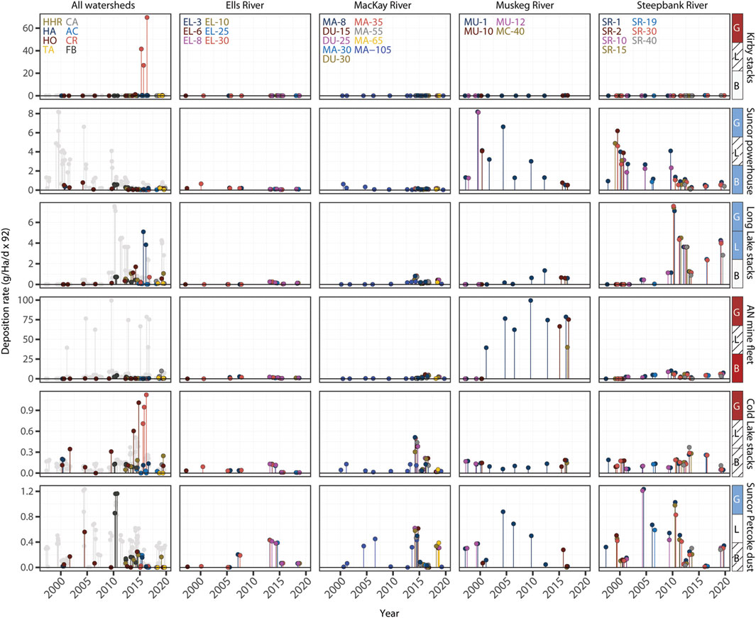
Figure 6. Examples of estimated deposition per fish watershed; coloured boxes on right indicate positive (red), negative (blue), neutral/less important (white), or unselected (hatched) for gonad mass (G), liver mass (L), or lethal body mass (B); light grey lollipops in all watersheds duplicate deposition estimates from the four focal watersheds; AN = Aurora North.
A main goal of the current analysis was to determine the potential effects of atmospheric deposition on fish health indicators. The results suggest both positive and negative effects on BM, LM, and GM associated with the estimated deposition of particles emitted from some facilities are occurring. Effects were observed across all industrial categories, such as mine and in situ stacks, mine dusts (mine areas, roads, petcoke piles), and mine fleet emissions. Climatic variables, wildfire area, and land disturbance were also associated with changes in indicators of fish health.
In this study, negative relationships were observed in multiple industrial variables and fish measurements, including mining and in situ stacks. For example, deposition of particles emitted from Suncor’s powerhouse were associated with negative effects on GM and BM of lethally-sampled fishes. Delayed petroleum coke is combusted at Suncor’s powerhouse and this activity is associated with the release of metals, sulphur, and organics (Tillman and Harding, 2004; Wang et al., 2012; Arciszewski, 2022). Other studies have also specifically highlighted the potential role of petcoke combustion in some of the patterns in chemical indicators, such as vanadium (V; Arciszewski, 2022) and in effects on benthic invertebrates (Arciszewski, 2021) and is generally suggested in other research (Gopalapillai et al., 2019).
There is additional information suggesting the effects of combusting delayed petroleum coke on the ambient environment in the OSR. While important effects in lethally-sampled fish were observed in response to the stacks at Suncor, no large or important effects in lethally-sampled fish were associated with the Mildred Lake stacks which upgrades bitumen using a fluid coker (Gray, 2015). Correspondingly, no effects of the Horizon stacks were observed in the lethal fish analyses which also uses delayed coking, but does not combust this material; however, emission from Horizon’s stacks were associated with negative effects in the EEM + FAM analyses of BM suggesting there may be small influences on fish. In combination, these data generally suggest the effects of combusting delayed petroleum coke compared to burning fluid coke or other fuels. However, this also contradicts other known relationships, including the greater emissions of some contaminants from Mildred Lake compared to Suncor, such as sulphur and some metals, such as Al, Ti, and Ni (Wang et al., 2012); patterns suggesting potential effects from Mildred Lake’s operations were not entirely absent suggesting some influence of fluid coking on the environment. However, many other stacks at other facilities, including a third upgrading type used for gasification and without a coker at Nexen until 2016 (Gray, 2015) were also associated with effects on fish. These observations highlight the potential effects of particles emitted from many types of stacks on the health of fish.
Additional information from this study also highlights more nuance in the potential effects of petroleum cokes. For example, there is also evidence suggesting dust emitted from Suncor and Horizon’s delayed petcoke stockpiles were each associated with negative effects in fish. Delayed petcoke dust has been found in the ambient environment in previous studies (Ahad et al., 2021) and its effects on fish suggested here may be associated with the same CoCs present in petcoke flyash (Tillmann and Harding 2004). In contrast, fluid coke dust emitted from Mildred Lake was not associated with important effects on lethally sampled fish (but was retained in the EEM + FAM3 BM model). The potential importance of emissions and deposition of dust particles from petcoke piles at facilities like Suncor and Horizon, but not Mildred Lake potentially highlights unique aspects of each substance. Fluid coke has low relative volatile content, higher surface area, and higher sulphur content compared to delayed coke, but these materials have similar (although not exact) profiles of metals (Zubot et al. 2012; Bryers, 1995). These characteristics suggest the volatiles and even minute differences in other contaminants found at greater concentration in delayed cokes may be more important predictors of negative effects on fish health. Additionally, fluid coke sequesters some contaminants, such as dissolved organics, but also leaches others, such as V and Mo during hydro-transport at Mildred Lake (Zubot et al. 2012). A potential interaction of fluid coke and other stressors was not examined here, but this mechanism may also be operating in the ambient environment.
Other negative effects were also identified in this study. Negative effects related to mine dusts may be associated with dissolution of particles in acidic waters (Barraza et al., 2024; Butt et al., 2024) and highlight the potential importance of post-deposition processes on the occurrence of effects in biota. Many other sources are potentially associated with negative responses in fish, but further and more specific analyses of particular stressors, such as laboratory exposures (Tetreault et al., 2003a) may eventually be required to disentangle these relationships.
Although some negative effects of atmospheric deposition predictors are suggested, such as a decrease in BM associated with Suncor’s powerhouse stack, positive effects (e.g., increased GM associated with Muskeg River stacks or Imperial Cold Lake and with Suncor’s FGD and “other” stacks) may also be occurring. Positive effects of some mine fleet emissions were also commonly observed. Nutrient enrichment has been observed in other indicators measured in the OSR (Wieder et al., 2016) and may be associated with nitrogen emitted in haul truck exhaust (Wang et al., 2016). Nitrogenous polycyclic aromatic compounds (NPACs) were not detected in sediments of a lake in a high-deposition zone prior to 1960s (Chibwe et al., 2020) and may also reflect the switch to truck-and-shovel mining which occurred in the early 1990s at Suncor and in 1999 at Syncrude (Arciszewski, 2022 and references therein). Modelled nitrogen deposition from 2009–2012 was often highest near the mines and supports this hypothesis (Hsu et al., 2016).
While nitrogen deposition is typically highest near the mines, these patterns are not always observed (Hsu et al., 2016). Spatial and temporal patchiness of deposition patterns were also estimated in our work, including petcoke from Suncor’s facility (Supplemental Figure S6) which supports earlier hypotheses of organics in sediments from Namur Lake (Kurek et al., 2013). Similarly, deposition of particles emitted from oil sands facilities likely occurs in the Peace-Athabasca Delta also supporting other work (Jautzy et al., 2015; Supplemental Figure S18) and suggesting deposition beyond 85–90 km from a source is routine (Hodson, 2013), but may be very challenging to detect in field samples measuring concentrations. These observations have additional implications for the design of future field programs and are discussed further below (See Section 4.3).
The magnitude of some of the calculated differences in fish endpoints estimated from the modeled scenarios (e.g., with and without the industrial stressors) are large suggesting the models may be mis-specified, but the results also suggest mean health metrics of fish captured across the region have improved over time. Although, for example, higher-than-normal condition may also have its own consequences (Müller et al., 2023), previous analyses of diatom communities in cores of lake sediments have attributed long-term changes to climate (Summers et al., 2016), but the analysis here suggested there were also differences attributable to industrial activity. Improved environmental performance of facilities and/or changing exposure scenarios, albeit over a much longer period than examined here, is also suggested by the decreased concentration of metals like V, Ni, Mo, and Ti in snow collected intermittently since the 1970s (e.g., Gopalapillai et al., 2019). The estimated deposition of particles emitted from some sources, such as Suncor’s powerhouse is also declining in the Muskeg and Steepbank rivers (Figure 6) further suggesting the environmental health of the OSR associated with atmospheric deposition of individual sources may be improving over time. Changes associated with large sources may partially be a response to intense and escalating scrutiny of the industry around 2009 to 2011 (Miall, 2013; Jajuee, 2014). The overall increase in the conditional (and regional) means of fish health indicators (and suggesting improvement) mirror other studies in the region on the numbers of spawning white sucker (Schwalb et al., 2015; Arciszewski et al., 2022a) and the size and relative abundance of white sucker and walleye in the Athabasca River (Arciszewski et al., 2017). The apparent (mean) improvements may, however, also be associated with the enrichment described above or with the counterbalancing of negative effects of some stressors. For example, the co-deposition of base cations neutralizing acidification is well-established (Fenn et al., 2015) and may be especially prevalent in low-elevation areas close to the mines (Arciszewski et al., 2022a).
There is, however, also evidence of collective negative effects of the atmospheric deposition at individual locations and regionally. For example, lower GSI is predicted among fish captured at the MU-1 site. If the persistent (and predicted) declines in GSI at sites like MU-1 are accurate, they may reflect greater deposition in the Muskeg River over time and may also mirror changes detected in residual conductivity in the same watershed over the same period (Arciszewski and Roberts, 2022). Patterns in the Muskeg River may also reflect greater deposition of novel compounds depositing in lakes near (but outside) the south-western margin of the Muskeg drainage (Chibwe et al., 2020). However, the extent of this pattern within the Muskeg proper is not yet known, but the deposition intensity in the Jackpine drainage (in the southwest Muskeg (Arciszewski, 2021) is among the highest in the study area and the watersheds examined here (Supplemental Figure S7). The mean relative difference in LSI, although increasing slightly, was also chronically below the critical effect size (Munkittrick et al., 2009) throughout the study period. Persistently low LSI may also reflect regional effects of subtle and widespread stressors observed in many studies, such as polyaromatic compounds (e.g., Kurek et al., 2013; Jautzy et al., 2015). Other data also suggests organic contaminants have been steadily rising over time in media like snow and lake sediments (e.g., Chibwe et al., 2021). The potential for local effects with a larger context of regional improvement may also partially corroborate the results of exposure studies done using snow (Parrott et al., 2018), but also suggest the value of repeated surveys at proximate locations over time. There is also some additional evidence from the current analysis (e.g., the results of the BM analyses differed by the dataset used (Figure 3)) suggesting the influence of spatial scale, along with other factors, on the analyses and the interpretation. These possibilities are discussed further below (See Section 4.3), but these scaling issues are common in terrestrial studies (Roberts et al., 2022a).
There are many industrial variables which were neither retained, selected, nor deemed more important in the final models. The lack of relevance of many individual industrial predictors along with others in the same class potentially negatively or positively affecting the health of fish may be associated with multiple factors. First, some individual sources within a class may have slightly different chemical or physical characteristics. For example, the petroleum coke stockpiled in the OSR is of two types: delayed (Suncor and Horizon) and fluid (Syncrude) and each is chemically and physically distinct (Bryers, 1995). Second, the qualities of bedrock and surficial geology vary throughout the region and may influence the variability from some sources, such as wind-blown mine dust and mechanically generated dust from roads (e.g., Spiers et al., 1989). Third, practices and approaches at each facility overlap, but they are ultimately distinct and have also not been static at a given facility over time (e.g., Wang et al., 2012; Gray, 2015; Small et al., 2015). While other factors, such as atmospheric transformation can also occur (Horb et al., 2022) and some stressors which portions may be toxicologically inert at the documented concentrations (Shotyk et al., 2021) or toxic under certain conditions (e.g., Barraza et al., 2024; Butt et al., 2024), in sum, these results suggest the chemical characteristics of deposited particles associated with classes of materials may not be uniform (Wang et al., 2015). However, understanding these (mean) differences, how they may differ over time, and documenting and disentangling these relationships may require substantial effort. Where and when fish samples were collected relative to observed deposition from each source (e.g., Figure 1) may also affect the results and further investigating any future adjustments to the sampling design may be warranted; this is further discussed below (see Section 4.3).
Other associations were also identified in this analysis. An association of greater land disturbances in hydrologically-connected areas with lower BM, coupled with no effects in GM or LM may reflect physical responses, such as more loading of suspended sediments, blocking of light, and reduced primary productivity in streams rather than a toxic, physiological effect. The relationship of greater BM with greater sunlight intensity may also support an explanation based on physical phenomena. Similarly, the negative association of greater precipitation with GM, and the potential delivery of CoCs to streams during greater rain events may also highlight a physical explanation. However, precipitation may also be associated with greater scouring and weathering of in-stream organics and minerals (e.g., Birks et al., 2017; Droppo et al., 2018). These results may highlight the potential need for incorporating instrumentation at some or all fish locations in a pilot study, such as more accurate measures of sunlight intensity via in situ radiometry to better understand the relationships between fish and modeled features.
The inconsistent finding between land disturbance among LM and GM with BM was also observed in previous work (Arciszewski, 2021; 2022). However, land disturbance was not consistently estimated between the current study and that previous work. In the current study, land disturbance per watershed is estimated after subtracting the hydrologically isolated areas from the human footprint inventory (Alberta Biodiversity Monitoring Institute, 2024). Some of the deposited material occurs in these hydrologically isolated areas (e.g., Supplemental Figure S3) and often the most intense deposition occurs in these areas, including the mine pits. Consequently, some areas of facilities may be sinks for materials emitted from the same facility, but may also capture particles emitted from others. Removing these hydrologically isolated areas from estimates of deposition (and estimating run-off) has not been done in other studies (Kelly et al., 2009; Wasiuta et al., 2019). While these previous studies may be over-estimating the diffuse run-off of deposited materials into local watersheds and some of this water may be retained in tailings or other ponds, some of this water may be shuttled to on-lease settling ponds and eventually discharged to streams (e.g., RAMP, 2010).
A primary and underlying result from this study was the utility of incorporating the influence of spatio-temporal fields into the analyses of fish data. Although common in some disciplines (e.g., Moraga, 2020), analyses of fish health data, including those done in Canada’s OSR have not previously used spatio-temporal random effects. The results suggest this modelling approach, coupled with the estimates of deposited particles emitted from industrial sites, accounts for variation in the fish measurements and may be more sensitive than previous work. Previous work on fish did not identify potentially relevant differences in the Steepbank River over time (Tetreault et al., 2020) and this may be related to the categorization of sites as “reference” or “exposure”. For example, large differences were detected here in GSI, LSI, and k at both reference and exposure sites sampled in the Steepbank and Muskeg Rivers prior to 2002; negative effects at the reference site could have masked negative effects at exposure sites when relative site-to-site comparisons are made. The current analytical approach may also harness information embedded in the design associated with the temporal blocking and spatial clustering of sampling for fish within reaches (e.g., most of the samples collected before 2001 were from the Steepbank River; e.g., Supplementary Table S1), the proximity of multiple locations to each other, and multiple sites per tributary. While other attempts have been made to overcome the categorization of sites by examining sites over time (Arciszewski et al., 2022b), those analyses still did not address the potential temporal or spatial auto-correlations associated with the study design. Along with using variables such as atmospheric deposition to define exposure gradients, utilizing spatial and temporal dimensions of samples may be a powerful addition to analyses of the necessarily regional and long-term datasets available in Canada’s OSR. Spatio-temporal analyses like those done here using INLA may also be easily applied to other datasets available in the OSR, including water quality (Arciszewski and Roberts, 2022) and benthic invertebrate communities (Arciszewski, 2021).
Capturing background variation has been a focus of much work on fish in the OSR in recent years (e.g., Kilgour et al., 2019; Arciszewski and McMaster, 2021; Arciszewski et al., 2022b; McMillan et al., 2022). Various approaches have been used and have highlighted some of the same phenomena we observed, including improvement of model fit by using features such as climate (Arciszewski et al., 2022b) and fish covariates capture most of the variability (e.g., Kilgour et al., 2019), the spatio-temporal random effects may also be an important addition to these regional analyses. More specifically, the spatio-temporal random effects likely reflect the influence of missing covariates, including the Julian Day samples are collected each year (these data were not available for all fish), the non-industrial waters discharged from mines and in situ facilities into tributaries (e.g., RAMP, 2010), and the background effects of factors like water temperature, discharge, and surficial and bedrock geology. Previous analysis suggests these factors are important (Arciszewski et al., 2022b), but these data are not always available. While some of these missing historical or contemporary data may be filled-in using models (e.g., Schofield et al., 2016), the spatio-temporal fields may compensate for missing covariates and may be especially important for large regional programs in which obtaining robust background data, such as water temperature may be cumbersome, expensive, and fragile (e.g., probes can be easily lost.) Spatio-temporal fields may be used where such data are missing for historical surveys, or where the representativeness of any existing “background” data is difficult to establish.
Although apparently beneficial, there are also some potential concerns with the spatio-temporal approach. For example, the spatial effects, such as the upstream bedrock and surficial geology, may be shared among the natural and anthropogenic stressors (Spiers et al., 1989; Headley et al., 2005; Hein and Cotterill, 2006). These effects may also be challenging to resolve, and, more generally, the spatio-temporal random effects may also be confounding other covariates in the current analysis. Setting constraints, such as orthogonality has been proposed to address spatio-temporal confounding effects, but there is debate on its effectiveness (Urdangarin et al., 2023). Some suggest skeptical priors may address some of these concerns in spatial models (Zimmerman and Ver Hoef, 2022), but future work could explicitly examine the use of orthogonal constraints or other options, such as restricted regression (Adin et al., 2023) on this and other analyses. More skeptical or other types of priors, such as shrinkage (Van Erp et al., 2019), or penalized complexity priors (Fuglstad et al., 2019) may also be useful to reduce spatio-temporal confounding effects if they are present. Many other spatio-temporal tools are available and may also be worth exploring (e.g., Fox et al., 2020).
Although including predictors like expected rates of atmospheric deposition provides information, the analyses also indicate that generic patterns can be identified in analyses which only include the spatio-temporal effects or those which include both climate and the spatio-temporal effects. There may also be benefits to pursuing analyzing monitoring data in the future with only spatio-temporal random effects and climate data. First, these models indicate lower relative BM in 1997, 1999, and 2000 (but higher in 2001) in the Steepbank and Muskeg Rivers (Supplemental Figure S19). Second, the removal of most predictors, including the atmospheric deposition can address uncertain assumptions of including these variables, such as their run-off rate. Third, providing accurate estimates of deposition may be technically challenging and may require many years to perfect; for example, emission sources from the City of Fort McMurray may also be required (e.g., Lynam et al., 2015). Fourth, measurements of relevant background indicators, such as discharge and water temperature are not available for all study locations and may also require modelling if these variables must be incorporated. Analyses using spatio-temporal random effects can, in contrast, be implemented immediately across a variety of indicators already being measured in the OSR, but these fields would describe complex structure.
The results discussed thus far are relevant in-and-of-themselves, but there are some potential challenges with the work. The largest challenge is the use of data collected for a different specific purpose than this spatio-temporal analysis. However, this study has also highlighted challenges with some of the current spatial analyses used elsewhere (Arciszewski et al., 2022b), such as the complexity of the stressor gradients. For example, the expected stressor patterns associated with proximity of sources and study sites do occur, but they are also likely accompanied by deposition from more remote facilities; and these patterns likely change within and among years. The stressor gradients are more diverse than initially considered in the design of many monitoring programs in the region (e.g., RAMP, 1999) and further suggest identifying reference sites (or determining what they are referencing) may be challenging.
Combining similar datasets, including the non-lethal EEM and the FAM data with the lethally sampled fish was explored here. Similar to previous work (Arciszewski et al., 2022b) the analyses here suggest BM is sensitive to industrial effects, but that adding additional data available from non-lethal programs may not be beneficial. The loss of some signals in the analyses using the non-lethal data compared to the lethal BM (e.g., Figure 3), may be associated with additional species, sites, years, or data density (in all cases > 50% of data were collected after 2012; Supplemental Figure S20). The re-appearance of small signals in the EEM + FAM3 analysis suggests a role of all 4, but also suggests the non-lethal and lethal datasets may not be easily combined. A deeper exploration of combining these lethal and non-lethal data may also be useful, including the potential down-weighting of the more abundant data collected after 2013/2014.
The spatio-temporal approach used here identified some potentially relevant patterns not identified in previous work. If future analyses intend to use a spatio-temporal approach, our results suggest some changes, adjustments, or modifications to the sampling designs may be prudent. Although it may be challenging to practically achieve, the broadening of sampling locations may allow for samples to be collected in areas with high deposition from particular sources. For example, although pilot surveys have been done, no fish samples collected using EEM protocols near the areas with the highest deposition of particles emitted from Imperial Cold Lake between 1997 and 2019 are available (Supplemental Figure S5). However, adding sites typically requires more time, money, and staff, but transitioning from strict site-based analyses, either upstream to downstream or site-specifically (Tetreault et al., 2020; Arciszewski et al., 2022b) to regional-based analysis may free these resources. Currently, repeat sampling at the same sites over time and minimum sample size requirements per site limit the existing designs and may be loosened. Additionally, spreading effort typically used for a single reach covering typically <500 m for 40 fish may be better spent over larger distances (e.g., ranges of Matérn correlations) with fewer fish per sub-reach (and per species where multiple sentinel species co-occur). A wholesale (or the most extreme shift to coordinates for each captured fish) shift is not likely beneficial, but a pilot study on some candidate locations and comparing the results with and without this new data may be warranted. However, as demonstrated by adding more data into the BM analyses (e.g., Figures 3, 5), more non-lethal sampling of slimy sculpin, lake chub, and longnose dace may not be beneficial but better understanding the reasons for this may also be worthwhile.
Along with sites near specific facilities (or intended to better capture the influence of emissions of a particular facility) adjustments to the study design can also be guided by additional information. Lethal collections can, for instance, be added at sites with high deposition and already included in the FAM program, such as the JC-25 and JC-50 locations (Supplemental Figures S1, 7). Sampling in areas with low deposition in the upper watersheds of some tributaries and adding paired sites which are physically proximate but separated by confluences of streams, such as the merging of the North Steepbank and Steepbank proper and the straddling of the SR-30 and SR-40 sites at that confluence (Figure 1) may also improve the sensitivity of future analyses to signals associated with atmospheric deposition. Additional sites may be selected from total mass deposition, but varied spatial and temporal patterns were estimated, including sites with little apparent change over time (e.g., TA-25; Supplemental Figure S7). Total mass deposition also highlights the typical similarities of deposition rates in the same drainage (Supplemental Figure S7). Additionally, more detailed and specific characterization of deposition patterns may also be required to optimize the design since not all downstream sites have a greater rate of deposition per unit area. For example, the CR-186 site is the second-most upstream location in the Christina River, but the HYSPLIT modelling suggests the most intense estimated deposition per unit area in that drainage from in 2015–2019 occurs at this site (Supplemental Figure S7). While useful for planning, deposition estimates may, however, be challenging to obtain a priori, but generic and relative estimates may be sufficient to capture the largest gradients. Finally, adding detailed information on factors like run-off and/or retention of particles in the landscape may further clarify the exposure scenarios. However, pursuing more and more rigorous modelling may be exceptionally challenging given concerns around the quality of the source data available for emissions (e.g., Walker, 2022) and in discrepancies between predicted and observed outcomes, such as acidification (Hazewinkel et al., 2008; Makar et al., 2018). These factors potentially highlight the challenges of meeting the specific needs of a regional program. Another approach is to use spatio-temporal modeling without additional covariates may be capable of identifying areas of high or low observations (Supplemental Figure S19), but detailed stressor data may be required for diagnosing causes. Any adjustments to the fish sampling design must also consider how those changes may alter the sensitivity of the study to other stressors, such as the periodic discharge of non-industrial wastewater from mines and in situ facilities (Arciszewski et al., 2022a). Future analyses may also explore the integration of other environmental data such as water or sediment quality where available (McMillan et al., 2022).
Although not presented in the main text, removing the estimated effects of industrial variables (atmospheric deposition and land disturbances) provided an estimate of fish health indicators in a “baseline” state (See Supplemental Figure S21). While the model terms may be mis-specified and the analyses can undoubtedly be improved, the results of these expected ranges are consistent with patterns observed elsewhere in Canada (Barrett et al., 2015), including the overlap of GSI and k, and the separation of LSI among male and female slimy sculpin captured in the fall (Brasfield et al., 2013). Applying these ranges to fish collected since 2019 may yield valuable insights and may also simplify any future analyses of fish health metrics (Arciszewski and Munkittrick, 2015), but may also be simplistic.
Industrial development in Canada’s Oil Sands Region influences the environment, but the results of biomonitoring have been inconsistent. To overcome some of the challenges with existing studies, we used both estimates of atmospheric deposition, other industrial and natural variables, and spatio-temporal modelling to determine if the anthropogenic stressors are influencing the health of fish. The results generally suggest the roles many sources of particles deposited to the landscape. The results of the modelling also suggest impacts to fish at some locations, including the lower Muskeg and Steepbank rivers, but also that overall, the mean of the fish health indicators increased between 1997 and 2019. The study also identified the potential impacts of individual sources, including both petcoke dust and particles emitted from Suncor’s stacks along with many others. The results further suggest modifications to the study design to optimize the spatio-temporal modelling approach, including re-allocating effort and using deposition modelling to identify sites across the multiple exposure gradients present. The results also reinforce the difficulties of clearly detecting effects of the oil sands industry on the ambient environment.
All data except a few fish collected in the 1990s are available on publicly accessible databases either noted specifically in the text or elsewhere (e.g., https://www.canada.ca/en/environment-climate-change/services/oil-sands-monitoring/monitoring-water-quality-alberta-oil-sands.html or https://www.alberta.ca/oil-sands-monitoring-program-scientific-papers-and-data. Modelled deposition data are available: 10.17632/nsxgs8392s.1. However, the raw data supporting the conclusions of this article will be made available by the authors, without undue reservation.
The animal study was approved by the Canadian Council on Animal Care (CCAC) approved Animal Use protocols issued by the National Water Research Institute Animal Care Committee and with Government of Alberta-issued Fish Research Licenses. The study was conducted in accordance with the local legislation and institutional requirements.
TA: Conceptualization, Data curation, Formal Analysis, Methodology, Writing–original draft, Writing–review and editing. EU: Data curation, Funding acquisition, Methodology, Writing–review and editing. GT: Data curation, Funding acquisition, Writing–review and editing. KH: Data curation, Funding acquisition, Writing–review and editing. MM: Data curation, Funding acquisition, Writing–review and editing.
The author(s) declare that financial support was received for the research, authorship, and/or publication of this article. Funding for this analysis was provided by the Oil Sands Monitoring program annual workplanning (W-LTM-S-5-2324 and W-LTM-S-5-2425).
Studies like this are not possible without years of effort to collect the data and also the effort and resolve to make those data available. We thank the participants of the PERD, the RAMP, the JOSM, and the OSM for collecting and providing these long-term data. We’re also thankful for researchers at the Atmospheric Research Laboratory for making HYSPLIT open access and for all the other data curators/provisioners/modellers who make their data publicly available. While this work was supported by the Oil Sands Monitoring program, the contents of this paper does not necessarily reflect an official position of the program or its sponsoring organizations.
The authors declare that the research was conducted in the absence of any commercial or financial relationships that could be construed as a potential conflict of interest.
All claims expressed in this article are solely those of the authors and do not necessarily represent those of their affiliated organizations, or those of the publisher, the editors and the reviewers. Any product that may be evaluated in this article, or claim that may be made by its manufacturer, is not guaranteed or endorsed by the publisher.
The Supplementary Material for this article can be found online at: https://www.frontiersin.org/articles/10.3389/fenvs.2024.1405357/full#supplementary-material
Adin, A., Goicoa, T., Hodges, J. S., Schnell, P. M., and Ugarte, M. D. (2023). Alleviating confounding in spatio-temporal areal models with an application on crimes against women in India. Stat. Model. 23, 9–30. doi:10.1177/1471082X211015452
Ahad, J. M. E., Pakdel, H., Labarre, T., Cooke, C. A., Gammon, P. R., and Savard, M. M. (2021). Isotopic analyses fingerprint sources of polycyclic aromatic compound-bearing dust in athabasca oil sands region snowpack. Environ. Sci. Technol. 55, 5887–5897. doi:10.1021/acs.est.0c08339
Alberta Biodiversity Monitoring Institute (2024). Human footprint inventory. Available at: https://abmi.ca/home/data-analytics/da-top/da-product-overview/Human-Footprint-Products/HF-inventory.html.
Arciszewski, T. J. (2021). Exploring the influence of industrial and climatic variables on communities of benthic macroinvertebrates collected in streams and lakes in Canada’s oil sands region. Environments 8, 123. doi:10.3390/environments8110123
Arciszewski, T. J. (2022). A re-analysis and review of elemental and polycyclic aromatic compound deposition in snow and lake sediments from Canada’s Oil Sands Region integrating industrial performance and climatic variables. Sci. Total Environ. 820, 153254. doi:10.1016/j.scitotenv.2022.153254
Arciszewski, T. J., Hazewinkel, R. R. O., and Dubé, M. G. (2022a). A critical review of the ecological status of lakes and rivers from Canada’s oil sands region. Integr Envir Assess Manag 18, 361–387. doi:10.1002/ieam.4524
Arciszewski, T. J., and McMaster, M. E. (2021). Potential influence of sewage phosphorus and wet and dry deposition detected in fish collected in the athabasca river north of fort mcmurray. Environ. - MDPI 8, 14–21. doi:10.3390/environments8020014
Arciszewski, T. J., and Munkittrick, K. R. (2015). Development of an adaptive monitoring framework for long-term programs: an example using indicators of fish health. Integr. Environ. Assess. Manag. 11, 701–718. doi:10.1002/ieam.1636
Arciszewski, T. J., Munkittrick, K. R., Kilgour, B. W., Keith, H. M., Linehan, J. E., and McMaster, M. E. (2017). Increased size and relative abundance of migratory fishes observed near the Athabasca oil sands. Facets 2, 833–858. doi:10.1139/facets-2017-0028
Arciszewski, T. J., and Roberts, D. R. (2022). Analyzing relationships of conductivity and alkalinity using historical datasets from streams in northern Alberta, Canada. Water 14, 2503. doi:10.3390/w14162503
Arciszewski, T. J., Ussery, E. J., and McMaster, M. E. (2022b). Incorporating industrial and climatic covariates into analyses of fish health indicators measured in a stream in Canada’s oil sands region. Environments 9, 73. doi:10.3390/environments9060073
Ashby, M. (2023). Sfhotspot: hot-spot analysis with simple features. Available at: https://CRAN.R-project.org/package=sfhotspot.
Barraza, F., Javed, M. B., Noernberg, T., Schultz, J., and Shotyk, W. (2024). Spatial variation and chemical reactivity of dusts from open-pit bitumen mining using trace elements in snow. Chemosphere 350, 141081. doi:10.1016/j.chemosphere.2023.141081
Barrett, T. J., Brasfield, S. M., Carroll, L. C., Doyle, M. A., van den Heuvel, M. R., and Munkittrick, K. R. (2015). Reproductive strategies and seasonal changes in the somatic indices of seven small-bodied fishes in Atlantic Canada in relation to study design for environmental effects monitoring. Environ. Monit. Assess. 187, 305. doi:10.1007/s10661-015-4496-4
Birks, S. J., Cho, S., Taylor, E., Yi, Y., and Gibson, J. J. (2017). Characterizing the PAHs in surface waters and snow in the Athabasca region: implications for identifying hydrological pathways of atmospheric deposition. Sci. Total Environ. 603 (604), 570–583. doi:10.1016/j.scitotenv.2017.06.051
Blanchard, D., Aherne, J., and Makar, P. (2021). Dissolved organic carbon in lakes of the athabasca oil sands region: is color an indicator of acid sensitivity? Environ. Sci. Technol. 55, 6791–6803. doi:10.1021/acs.est.1c00507
Blangiardo, M., and Cameletti, M. (2015). Spatial and spatio-temporal bayesian models with R-INLA. 1st Edn. Wiley. doi:10.1002/9781118950203
Brasfield, S. M., Tetreault, G. R., McMaster, M. E., Bennett, J., and Munkittrick, K. R. (2013). Seasonal patterns of gonad size, liver size, and in vitro gonadal steroidogenic capacity in slimy sculpin (Cottus cognatus). Water Qual. Res. J. Can. 48, 243–254. doi:10.2166/wqrjc.2013.048
Bryers, R. W. (1995). Utilization of petroleum coke and petroleum coke/coal blends as a means of steam raising. Fuel Process. Technol. 44, 121–141. doi:10.1016/0378-3820(94)00118-D
Bullock, O. R., and Brehme, K. A. (2002). Atmospheric mercury simulation using the CMAQ model: formulation description and analysis of wet deposition results. Atmos. Environ. 36, 2135–2146. doi:10.1016/S1352-2310(02)00220-0
Butt, S. A., Barraza, F., Devito, K., Frost, L., Javed, M. B., Noernberg, T., et al. (2024). Spatio-temporal variations in dissolved trace elements in peat bog porewaters impacted by dust inputs from open-pit mining activities in the Athabasca Bituminous Sands (ABS) region. Environ. Pollut. 345, 123470. doi:10.1016/j.envpol.2024.123470
Chen, B., Stein, A. F., Maldonado, P. G., Sanchez De La Campa, A. M., Gonzalez-Castanedo, Y., Castell, N., et al. (2013). Size distribution and concentrations of heavy metals in atmospheric aerosols originating from industrial emissions as predicted by the HYSPLIT model. Atmos. Environ. 71, 234–244. doi:10.1016/j.atmosenv.2013.02.013
Chibwe, L., Muir, D. C. G., Gopalapillai, Y., Shang, D., Kirk, J. L., Manzano, C. A., et al. (2021). Long-term spatial and temporal trends, and source apportionment of polycyclic aromatic compounds in the Athabasca Oil Sands Region. Environ. Pollut. 268, 115351. doi:10.1016/j.envpol.2020.115351
Chibwe, L., Roberts, S., Shang, D., Yang, F., Manzano, C. A., Wang, X., et al. (2020). A one-century sedimentary record of N- and S-polycyclic aromatic compounds in the Athabasca oil sands region in Canada. Chemosphere 260, 127641. doi:10.1016/j.chemosphere.2020.127641
Cho, S., Sharma, K., Brassard, B. W., and Hazewinkel, R. (2014). Polycyclic aromatic hydrocarbon deposition in the snowpack of the Athabasca oil sands region of Alberta, Canada. Water, Air, Soil Pollut. 225, 1910. doi:10.1007/s11270-014-1910-4
Culp, J. M., Droppo, I. G., di Cenzo, P., Alexander, A. C., Baird, D. J., Beltaos, S., et al. (2021). Ecological effects and causal synthesis of oil sands activity impacts on river ecosystems: water synthesis review. Environ. Rev. 29, 315–327. doi:10.1139/er-2020-0082
Draxler, R. R., Ginoux, P., and Stein, A. F. (2010). An empirically derived emission algorithm for wind-blown dust. J. Geophys. Res. 115, 2009JD013167. doi:10.1029/2009JD013167
Droppo, I. G., di Cenzo, P., Power, J., Jaskot, C., Chambers, P. a., Alexander, A. C., et al. (2018). Temporal and spatial trends in riverine suspended sediment and associated polycyclic aromatic compounds (PAC) within the Athabasca oil sands region. Sci. Total Environ. 626, 1382–1393. doi:10.1016/j.scitotenv.2018.01.105
Emmerton, C. A., Cooke, C. A., Hustins, S., Silins, U., Emelko, M. B., Lewis, T., et al. (2020). Severe western Canadian wildfire affects water quality even at large basin scales. Water Res. 183, 116071. doi:10.1016/j.watres.2020.116071
Evans, M., Davies, M., Janzen, K., Muir, D., Hazewinkel, R., Kirk, J., et al. (2016). PAH distributions in sediments in the oil sands monitoring area and western Lake Athabasca: concentration, composition and diagnostic ratios. Environ. Pollut. 213, 671–687. doi:10.1016/j.envpol.2016.03.014
Fenn, M. E., Bytnerowicz, A., Schilling, S. L., and Ross, C. S. (2015). Atmospheric deposition of nitrogen, sulfur and base cations in jack pine stands in the Athabasca Oil Sands Region, Alberta, Canada. Environ. Pollut. 196, 497–510. doi:10.1016/j.envpol.2014.08.023
Fernie, K. J., Marteinson, S. C., Chen, D., Eng, A., Harner, T., Smits, J. E. G., et al. (2018). Elevated exposure, uptake and accumulation of polycyclic aromatic hydrocarbons by nestling tree swallows (Tachycineta bicolor) through multiple exposure routes in active mining-related areas of the Athabasca oil sands region. Sci. Total Environ. 624, 250–261. doi:10.1016/j.scitotenv.2017.12.123
Fox, E. W., Ver Hoef, J. M., and Olsen, A. R. (2020). Comparing spatial regression to random forests for large environmental data sets. PLoS ONE 15, e0229509. doi:10.1371/journal.pone.0229509
Fuglstad, G.-A., Simpson, D., Lindgren, F., and Rue, H. (2019). Constructing priors that penalize the complexity of Gaussian random fields. J. Am. Stat. Assoc. 114, 445–452. doi:10.1080/01621459.2017.1415907
Gelman, A., Carlin, J. B., Stern, H. S., Dunson, D. B., Vehtari, A., and Rubin, D. B. (2013). Bayesian data analysis. Chapman and Hall/CRC.
Gerner, N. V., Koné, M., Ross, M. S., Pereira, A., Ulrich, A. C., Martin, J. W., et al. (2017). Stream invertebrate community structure at Canadian oil sands development is linked to concentration of bitumen-derived contaminants. Sci. Total Environ. 575, 1005–1013. doi:10.1016/j.scitotenv.2016.09.169
Gopalapillai, Y., Kirk, J. L., Landis, M. S., Muir, D. C. G., Cooke, C. A., Gleason, A., et al. (2019). Source analysis of pollutant elements in winter air deposition in the athabasca oil sands region: a temporal and spatial study. ACS Earth Space Chem. 3, 1656–1668. doi:10.1021/acsearthspacechem.9b00150
Government of Alberta (2024a). Alberta climate information service (ACIS) data products and tools. Available at: https://www.acis.alberta.ca/acis/(Accessed July 24, 2023).
Government of Alberta (2024b). Wildfire maps and data. Available at: https://www.alberta.ca/wildfire-maps-and-data (Accessed August 15, 2023).
Gray, M. A., Curry, A. R., and Munkittrick, K. R. (2002). Non-lethal sampling methods for assessing environmental impacts using a small-bodied sentinel fish species. Water Qual. Res. J. Can. 37, 195–211. doi:10.2166/wqrj.2002.012
Gray, M. R. (2015). Upgrading oilsands bitumen and heavy oil. Edmonton, Alberta: University of Alberta.
Harner, T., Rauert, C., Muir, D., Schuster, J. K., Hsu, Y. M., Zhang, L., et al. (2018). Air synthesis review: polycyclic aromatic compounds in the oil sands region. Environ. Rev. 26, 430–468. doi:10.1139/er-2018-0039
Harrell, F. E. (2015). Regression modeling strategies: with applications to linear models, logistic and ordinal regression, and survival analysis. Springer.
Hazewinkel, R. R. O., Wolfe, A. P., Pla, S., Curtis, C., and Hadley, K. (2008). Have atmospheric emissions from the Athabasca Oil Sands impacted lakes in northeastern Alberta, Canada? Can. J. Fish. Aquatic Sci. 65, 1554–1567. doi:10.1139/f08-074
Headley, J. V., Crosley, B., Conly, F. M., and Quagraine, E. K. (2005). The characterization and distribution of inorganic chemicals in tributary waters of the lower Athabasca River, oilsands region, Canada. J. Environ. Sci. Health, Part A 40, 1–27. doi:10.1081/ESE-200033418
Hein, F. J., and Cotterill, D. K. (2006). The athabasca oil sands — a regional geological perspective, fort McMurray area, Alberta, Canada. Nat. Resour. Res. 15, 85–102. doi:10.1007/s11053-006-9015-4
Hey, T., Tansley, S., and Tolle, K. M. (2009). The fourth paradigm: data-intensive scientific discovery. Redmond, WA: Microsoft Research.
Hodson, P. V. (2013). History of environmental contamination by oil sands extraction. Proc. Natl. Acad. Sci. U.S.A. 110, 1569–1570. doi:10.1073/pnas.1221660110
Horb, E. C., Wentworth, G. R., Makar, P. A., Liggio, J., Hayden, K., Boutzis, E. I., et al. (2022). A decadal synthesis of atmospheric emissions, ambient air quality, and deposition in the oil sands region. Integr Envir Assess Manag 18, 333–360. doi:10.1002/ieam.4539
Hsu, Y.-M., Bytnerowicz, A., Fenn, M. E., and Percy, K. E. (2016). Atmospheric dry deposition of sulfur and nitrogen in the athabasca oil sands region, Alberta, Canada. Sci. Total Environ. 568, 285–295. doi:10.1016/j.scitotenv.2016.05.205
Iannone, R. (2016). splitr. Available at: https://github.com/rich-iannone/splitr.
Jajuee, B. A. (2014). “Canada’s oil sands innovation alliance: delivering environmental performance,” in Day 1 Mon, march 17, 2014, (long beach, California, USA: spe), D011S013R006. doi:10.2118/168355-MS
Jautzy, J. J., Ahad, J. M. E., Gobeil, C., Smirnoff, A., Barst, B. D., and Savard, M. M. (2015). Isotopic evidence for oil sands petroleum coke in the peace–athabasca Delta. Environ. Sci. Technol. 49, 12062–12070. doi:10.1021/acs.est.5b03232
Kelly, E. N., Short, J. W., Schindler, D. W., Hodson, P. V., Ma, M., Kwan, A. K., et al. (2009). Oil sands development contributes polycyclic aromatic compounds to the Athabasca River and its tributaries. Proc. Natl. Acad. Sci. U.S.A. 106, 22346–22351. doi:10.1073/pnas.0912050106
Kilgour, B. W., Munkittrick, K. R., Hamilton, L., Proulx, C. L., Somers, K. M., Arciszewski, T., et al. (2019). Developing triggers for environmental effects monitoring programs for trout-perch in the lower Athabasca River (Canada). Environ. Toxicol. Chem. 38, 1890–1901. doi:10.1002/etc.4469
Kirk, J. L., Muir, D. C. G. G., Gleason, A., Wang, X., Lawson, G., Frank, R. A., et al. (2014). Atmospheric deposition of mercury and methylmercury to landscapes and waterbodies of the athabasca oil sands region. Environ. Sci. Technol. 48, 7374–7383. doi:10.1021/es500986r
Krainski, E., Gómez-Rubio, V., Bakka, H., Lenzi, A., Castro-Camilo, D., Simpson, D., et al. (2018). Advanced spatial modeling with stochastic partial differential equations using R and INLA. 0 Edn. Chapman and Hall/CRC. doi:10.1201/9780429031892
Kurek, J., Kirk, J. L., Muir, D. C. G. G., Wang, X., Evans, M. S., and Smol, J. P. (2013). Legacy of a half century of Athabasca oil sands development recorded by lake ecosystems. Proc. Natl. Acad. Sci. 110, 1761–1766. doi:10.1073/pnas.1217675110
Landis, M. S., Studabaker, W. B., Patrick Pancras, J., Graney, J. R., Puckett, K., White, E. M., et al. (2019). Source apportionment of an epiphytic lichen biomonitor to elucidate the sources and spatial distribution of polycyclic aromatic hydrocarbons in the Athabasca Oil Sands Region, Alberta, Canada. Sci. Total Environ. 654, 1241–1257. doi:10.1016/j.scitotenv.2018.11.131
Lindgren, F., Rue, H., and Lindström, J. (2011). An explicit link between Gaussian fields and Gaussian Markov random fields: the stochastic partial differential equation approach. J. R. Stat. Soc. Ser. B Stat. Methodol. 73, 423–498. doi:10.1111/j.1467-9868.2011.00777.x
Lynam, M. M., Dvonch, J. T., Barres, J. A., Morishita, M., Legge, A., and Percy, K. (2015). Oil sands development and its impact on atmospheric wet deposition of air pollutants to the Athabasca Oil Sands Region, Alberta, Canada. Alberta: Canada. Environ. 206, 469–478. doi:10.1016/j.envpol.2015.07.032
Makar, P. A., Akingunola, A., Aherne, J., Cole, A. S., Aklilu, Y., Zhang, J., et al. (2018). Estimates of exceedances of critical loads for acidifying deposition in Alberta and Saskatchewan. Atmos. Chem. Phys. 18, 9897–9927. doi:10.5194/acp-18-9897-2018
McElreath, R. (2018). Statistical rethinking: a bayesian course with examples in R and stan. 1st Edn. Chapman and Hall/CRC. doi:10.1201/9781315372495
McMillan, P. G., Feng, Z. Z., Deeth, L. E., and Arciszewski, T. J. (2022). Improving monitoring of fish health in the oil sands region using regularization techniques and water quality variables. Sci. Total Environ. 811, 152301. doi:10.1016/j.scitotenv.2021.152301
Miall, A. D. (2013). Geoscience of climate and energy 10. The Alberta oil sands: developing a new regime of environmental management, 2010–2013. GS 40, 174. doi:10.12789/geocanj.2013.40.015
Moraga, P. (2020). Geospatial health data: modeling and visualization with R-INLA and Shiny. Boca Raton, FL: CRC Press.
Moroz, B. E., Beck, H. L., Bouville, A., and Simon, S. L. (2010). PREDICTIONS OF DISPERSION AND DEPOSITION OF FALLOUT FROM NUCLEAR TESTING USING THE NOAA-HYSPLIT METEOROLOGICAL MODEL. Health Phys. 99, 252–269. doi:10.1097/HP.0b013e3181b43697
Mullan-Boudreau, G., Belland, R., Devito, K., Noernberg, T., Pelletier, R., and Shotyk, W. (2017). Sphagnum moss as an indicator of contemporary rates of atmospheric dust deposition in the athabasca bituminous sands region. Environ. Sci. Technol. 51, 7422–7431. doi:10.1021/acs.est.6b06195
Müller, J., Houben, N., and Pauly, D. (2023). On being the wrong size, or the role of body mass in fish kills and hypoxia exposure. Environ. Biol. Fishes 106, 1651–1667. doi:10.1007/s10641-023-01442-w
Mundy, L. J., Bilodeau, J. C., Schock, D. M., Thomas, P. J., Blais, J. M., Pauli, B. D., et al. (2019). Using wood frog (Lithobates sylvaticus) tadpoles and semipermeable membrane devices to monitor polycyclic aromatic compounds in boreal wetlands in the oil sands region of northern Alberta, Canada. Chemosphere 214, 148–157. doi:10.1016/j.chemosphere.2018.09.034
Munkittrick, K. R., Arens, C. J., Lowell, R. B., and Kaminski, G. P. (2009). A review of potential methods of determining critical effect size for designing environmental monitoring programs. Environ. Toxicol. Chem. 28, 1361–1371. doi:10.1897/08-376.1
Oil Sands Magazine (2024). Oil sands operations | oil sands magazine. Available at: https://www.oilsandsmagazine.com/projects/bitumen-production (Accessed March 16, 2024).
Parrott, J. L., Marentette, J. R., Hewitt, L. M., McMaster, M. E., Gillis, P. L., Norwood, W. P., et al. (2018). Meltwater from snow contaminated by oil sands emissions is toxic to larval fish, but not spring river water. Sci. Total Environ. 625, 264–274. doi:10.1016/j.scitotenv.2017.12.284
Parsons, B. G., Watmough, S. A., Dillon, P. J., and Somers, K. M. (2010). A bioassessment of lakes in the Athabasca Oil Sands Region, Alberta, using benthic macroinvertebrates. J. Limnol. 69, 105–117. doi:10.4081/jlimnol.2010.s1.105
RAMP (1999). Regional aquatics monitoring program 1999 technical report. Available at: http://www.ramp-alberta.org/ramp/results/report.aspx.
RAMP (2009). Regional aquatics monitoring program 2009 technical report. Available at: http://www.ramp-alberta.org/ramp/results/report.aspx.
RAMP (2010). Regional aquatics monitoring program 2010 technical report. Available at: http://www.ramp-alberta.org/ramp/results/report.aspx.
Roberts, D. R., Bayne, E. M., Beausoleil, D., Dennett, J., Fisher, J. T., Hazewinkel, R. O., et al. (2022a). A synthetic review of terrestrial biological research from the Alberta oil sands region: 10 years of published literature. Integr Envir Assess Manag 18, 388–406. doi:10.1002/ieam.4519
Roberts, D. R., Hazewinkel, R. O., Arciszewski, T. J., Beausoleil, D., Davidson, C. J., Horb, E. C., et al. (2022b). An integrated knowledge synthesis of regional ambient monitoring in Canada’s oil sands. Integr Envir Assess Manag 18, 428–441. doi:10.1002/ieam.4505
Rue, H., Martino, S., and Chopin, N. (2009). Approximate bayesian inference for latent Gaussian models by using integrated nested Laplace approximations. J. R. Stat. Soc. Ser. B Stat. Methodol. 71, 319–392. doi:10.1111/j.1467-9868.2008.00700.x
Rue, H., Martino, S., Lindgren, F., Simpson, D., Riebler, A., and Krainski, E. T. (2014). INLA: functions which allow to perform full Bayesian analysis of latent Gaussian models using Integrated Nested Laplace Approximaxion. R. package version 0.0-1404466487. Available at: http://www.R-INLA.org.
Santos-Fernandez, E., Ver Hoef, J. M., Peterson, E. E., McGree, J., Isaak, D. J., and Mengersen, K. (2022). Bayesian spatio-temporal models for stream networks. Comput. Statistics Data Analysis 170, 107446. doi:10.1016/j.csda.2022.107446
Schade, G. W., and Gregg, M. L. (2022). Testing HYSPLIT plume dispersion model performance using regional hydrocarbon monitoring data during a gas well blowout. Atmosphere 13, 486. doi:10.3390/atmos13030486
Schofield, M. R., Barker, R. J., Gelman, A., Cook, E. R., and Briffa, K. R. (2016). A model-based approach to climate reconstruction using tree-ring data. J. Am. Stat. Assoc. 111, 93–106. doi:10.1080/01621459.2015.1110524
Schwalb, A. N., Alexander, A. C., Paul, A. J., Cottenie, K., and Rasmussen, J. B. (2015). Changes in migratory fish communities and their health, hydrology, and water chemistry in rivers of the Athabasca oil sands region: a review of historical and current data. Environ. Rev. 23, 133–150. doi:10.1139/er-2014-0065
Shotyk, W., Appleby, P. G., Bicalho, B., Davies, L. J., Froese, D., Grant-Weaver, I., et al. (2017). Peat bogs document decades of declining atmospheric contamination by trace metals in the athabasca bituminous sands region. Environ. Sci. Technol. 51, 6237–6249. doi:10.1021/acs.est.6b04909
Shotyk, W., Bicalho, B., Cuss, C., Donner, M., Grant-Weaver, I., Javed, M. B., et al. (2021). Trace elements in the Athabasca Bituminous Sands: a geochemical explanation for the paucity of environmental contamination by chalcophile elements. Chem. Geol. 581, 120392. doi:10.1016/j.chemgeo.2021.120392
Small, C. C., Cho, S., Hashisho, Z., and Ulrich, A. C. (2015). Emissions from oil sands tailings ponds: review of tailings pond parameters and emission estimates. J. Petroleum Sci. Eng. 127, 490–501. doi:10.1016/j.petrol.2014.11.020
Spiers, G. A., Dudas, M. J., and Turchenek, L. W. (1989). The chemical and mineralogical composition of soil parent materials in northeast Alberta. Can. J. Soil Sci. 69, 721–737. doi:10.4141/cjss89-074
Stein, A. F., Draxler, R. R., Rolph, G. D., Stunder, B. J. B., Cohen, M. D., and Ngan, F. (2015). NOAA’s HYSPLIT atmospheric transport and dispersion modeling system. Bull. Am. Meteorological Soc. 96, 2059–2077. doi:10.1175/BAMS-D-14-00110.1
Summers, J. C., Kurek, J., Kirk, J. L., Muir, D. C. G., Wang, X., Wiklund, J. A., et al. (2016). Recent warming, rather than industrial emissions of bioavailable nutrients, is the dominant driver of lake primary production shifts across the athabasca oil sands region. PloS one 11, 01539877–e154020. doi:10.1371/journal.pone.0153987
Sunderland, E. M., Cohen, M. D., Selin, N. E., and Chmura, G. L. (2008). Reconciling models and measurements to assess trends in atmospheric mercury deposition. Environ. Pollut. 156, 526–535. doi:10.1016/j.envpol.2008.01.021
Tetreault, G. R., Bennett, C. J., Clark, T. W., Keith, H., Parrott, J. L., and McMaster, M. E. (2020). Fish performance indicators adjacent to oil sands activity: response in performance indicators of slimy sculpin in the Steepbank River, Alberta, adjacent to oil sands mining activity. Environ. Toxicol. Chem. 39, 396–409. doi:10.1002/etc.4625
Tetreault, G. R., McMaster, M. E., Dixon, D. G., and Parrott, J. L. (2003a). Physiological and biochemical responses of ontario slimy sculpin (Cottus cognatus) to sediment from the athabasca oil sands area. Water Qual. Res. J. Can. 38, 361–377. doi:10.2166/wqrj.2003.023
Tetreault, G. R., McMaster, M. E., Dixon, D. G., and Parrott, J. L. (2003b). Using reproductive endpoints in small forage fish species to evaluate the effects of Athabasca Oil Sands activities. Environ. Toxicol. Chem. 22, 2775–2782. doi:10.1897/03-7
Tillman, D., and Harding, N. S. (2004). Fuels of opportunity: characteristics and uses in combustion systems. Elsevier.
Urdangarin, A., Goicoa, T., and Ugarte, M. D. (2023). Evaluating recent methods to overcome spatial confounding. Rev. Mat. Complut. 36, 333–360. doi:10.1007/s13163-022-00449-8
Van Erp, S., Oberski, D. L., and Mulder, J. (2019). Shrinkage priors for Bayesian penalized regression. J. Math. Psychol. 89, 31–50. doi:10.1016/j.jmp.2018.12.004
Walker, T. R. (2022). Effectiveness of the national pollutant release inventory as a policy tool to curb atmospheric industrial emissions in Canada. Pollutants 2, 289–305. doi:10.3390/pollutants2030019
Wang, X., Chow, J. C., Kohl, S. D., Percy, K. E., Legge, A. H., and Watson, J. G. (2015). Characterization of PM 2.5 and PM 10 fugitive dust source profiles in the athabasca oil sands region. J. Air and Waste Manag. Assoc. 65, 1421–1433. doi:10.1080/10962247.2015.1100693
Wang, X., Chow, J. C., Kohl, S. D., Percy, K. E., Legge, A. H., and Watson, J. G. (2016). Real-world emission factors for Caterpillar 797B heavy haulers during mining operations. Particuology 28, 22–30. doi:10.1016/j.partic.2015.07.001
Wang, X. L., Watson, J. G., Chow, J. C., Kohl, S. D., Chen, L.-W. A., Sodeman, D. A., et al. (2012). “Measurement of real-world stack emissions with a dilution sampling system,” in Developments in environmental science (Elsevier), 171–192. doi:10.1016/B978-0-08-097760-7.00008-1
Wasiuta, V., Kirk, J. L., Chambers, P. A., Alexander, A. C., Wyatt, F. R., Rooney, R. C., et al. (2019). Accumulating mercury and methylmercury burdens in watersheds impacted by oil sands pollution. Environ. Sci. Technol. 53, 12856–12864. doi:10.1021/acs.est.9b02373
Wieder, R. K., Scott, K. D., Vile, M. A., and Herron, C. (2022). Are bog plant/lichen tissue concentrations of Ca, Mg, K, and P affected by fugitive dust released from oil sands development in the Fort McMurray region of Alberta? Sci. Total Environ. 849, 157684. doi:10.1016/j.scitotenv.2022.157684
Wieder, R. K., Vile, M. A., Albright, C. M., Scott, K. D., Vitt, D. H., Quinn, J. C., et al. (2016). Effects of altered atmospheric nutrient deposition from Alberta oil sands development on Sphagnum fuscum growth and C, N and S accumulation in peat. Biogeochemistry 129, 1–19. doi:10.1007/s10533-016-0216-6
Wynia, A. G., Tetreault, G. R., Clark, T. W., Cunningham, J. L., Ussery, E. J., and McMaster, M. E. (2022). Fish assemblage monitoring in Alberta’s Ells River: baseline fish and habitat variability prior to major development. Glob. Ecol. Conservation 34, e02007. doi:10.1016/j.gecco.2022.e02007
Zimmerman, D. L., and Ver Hoef, J. M. (2022). On deconfounding spatial confounding in linear models. Am. Statistician 76, 159–167. doi:10.1080/00031305.2021.1946149
Zuur, A. F., Ieno, E. N., Savelʹev, A. A., and Zuur, A. F. (2017). Beginner’s guide to spatial, temporal and spatial-temporal ecological data analysis with R-INLA Volume I: using GLM and GLMM. Newburgh, United Kingdom: Highland Statistics Ltd.
Keywords: fish health, oil sands, atmospheric deposition, spatio-temporal modelling, climate, INLA, HYSPLIT
Citation: Arciszewski TJ, Ussery EJ, Tetreault GR, Hicks KA and McMaster ME (2024) Assessing changes in indicators of fish health measured between 1997 and 2019 relative to multiple natural and anthropogenic stressors in Canada’s oil sands region using spatio-temporal modeling. Front. Environ. Sci. 12:1405357. doi: 10.3389/fenvs.2024.1405357
Received: 22 March 2024; Accepted: 18 June 2024;
Published: 18 July 2024.
Edited by:
Rui Zhang, University of Jinan, ChinaReviewed by:
Song Fanhao, Chinese Research Academy of Environmental Sciences, ChinaCopyright © 2024 Arciszewski, Ussery, Tetreault, Hicks and McMaster. This is an open-access article distributed under the terms of the Creative Commons Attribution License (CC BY). The use, distribution or reproduction in other forums is permitted, provided the original author(s) and the copyright owner(s) are credited and that the original publication in this journal is cited, in accordance with accepted academic practice. No use, distribution or reproduction is permitted which does not comply with these terms.
*Correspondence: Tim J. Arciszewski, dGltLmFyY2lzemV3c2tpQGdtYWlsLmNvbQ==
Disclaimer: All claims expressed in this article are solely those of the authors and do not necessarily represent those of their affiliated organizations, or those of the publisher, the editors and the reviewers. Any product that may be evaluated in this article or claim that may be made by its manufacturer is not guaranteed or endorsed by the publisher.
Research integrity at Frontiers
Learn more about the work of our research integrity team to safeguard the quality of each article we publish.