 Nan Lin
 Xianjun Mei1,2
94% of researchers rate our articles as excellent or good
Learn more about the work of our research integrity team to safeguard the quality of each article we publish.
Find out more
ORIGINAL RESEARCH article
Front. Environ. Sci., 27 June 2024
Sec. Environmental Informatics and Remote Sensing
Volume 12 - 2024 | https://doi.org/10.3389/fenvs.2024.1401107
Introduction: Fast and accurate estimation and spatial mapping of soil total nitrogen (TN) content is important for the development of modern precision agriculture, such as soil fertility monitoring and land reclamation decision-making. Hyperspectral remote sensing has been demonstrated to be an accurate real-time technique for rapid estimation and mapping of soil TN content.
Methods: To solve the problem of poor accuracy and generalization of estimation models caused by soil environmental heterogeneity in estimating and mapping soil TN content using hyperspectral images, 502 soil samples were collected from a typical black soil area in Yushu City, Jilin Province, China, as a test area, and three sample grouping strategies were established by soil environmental variables (soil type, thickness of the black soil layer, and topographic factors), and Pearson correlation coefficient and competitive adaptive reweighted sampling algorithm were used to determine the TN characteristic bands of each sample set under different strategies. Based on the data characteristics of the sub-sample set, the local regression estimation model based on sample grouping was constructed using the CatBoost algorithm, and the estimation and distribution mapping of soil TN content was carried out.
Results and Discussion: The results showed that after dividing the samples according to the differences in soil environmental factors, the characteristic information of the samples is more targeted, with more abundant numbers and distribution ranges of TN characteristic bands. Compared to the global regression estimation with all samples, the local regression based on the grouping of soil environment differences showed improved accuracy, with the local regression estimation model constructed with the ST-G strategy exhibiting the highest estimation accuracy (
Soil is an indispensable part of the Earth’s ecosystem, with a complex structure and multiple functions (Du and Zhou, 2009). It provides water, minerals, and nutrients such as organic matter, nitrogen, phosphorus, and potassium to plants and soil organisms, playing a key role in climate regulation, vegetation growth, and maintenance of ecological balance (Wilding and Lin, 2006). Soil nitrogen is closely related to soil aggregate formation, microbial metabolism, and changes in soil texture (Li et al., 2022). It is an important nutrient element affecting and limiting plant growth and development and a key element in regulating soil fertility, quality, and agricultural productivity (Lori et al., 2018). Therefore, determining total nitrogen (TN) content in soil and its spatial distribution is important for soil fertility monitoring, land resource management, and sustainable agricultural development (Peng et al., 2021). The traditional soil chemical analysis method can obtain accurate information on soil TN content. However, it requires much time, effort and cost, and detailed information on TN content is not possible on a large scale (Sinfield et al., 2010). The field spectrum measurement using proximal sensors can invert the chemical composition of the soil according to its reflection characteristics and physical and chemical properties, enabling rapid and accurate estimation of the content of various soil components such as organic matter and TN (Yang et al., 2012; Kawamura et al., 2017; Jiang et al., 2023a). However, this method is dependent on point locations, making it difficult to obtain dynamic and continuous spatial distribution information of soil TN content through ground spectral data. Therefore, a fast and accurate method needs to be developed to dynamically obtain the spatial distribution of TN content on a large scale.
Since the stretching and cornering vibrations of many functional groups (N-H, N-C, and N≡N bonds) in soils induce specific spectral response and absorption radiance in the soil reflectance curves, a certain correlation can be identified between TN content and soil spectrum (Stenberg and Rossel, 2010; Zhang and He, 2016). This correlation provides a study basis for the estimation and mapping of soil TN content. With wide coverage, fast information acquisition, and strong timeliness, hyperspectral satellite remote sensing has been largely applied to large-scale soil nutrient estimation, soil characteristic evaluation, and digital soil mapping (Grunwald et al., 2015; Chatterjee et al., 2021; Xu et al., 2023). Currently, soil TN content estimation and mapping by hyperspectral images mainly focuses on hyperspectral data preprocessing, feature variable selection, and estimation model construction, etc. Many studies have demonstrated that imagery preprocessing, such as radiation and atmospheric correction, can effectively reduce or eliminate noise in spectral data acquisition (Minu et al., 2017; Minu et al., 2018; Wang J. et al., 2022). By mathematically converting spectral reflectance, spectral information related to soil nutrients can be enhanced, and the effects of interference factors can be suppressed or eliminated (Hong et al., 2019; Zhang et al., 2020). By selecting appropriate spectral feature bands by feature selection algorithms (e.g., the LASSO algorithm, the successive projections algorithm, the uninformative variable elimination, and the genetic algorithm), the data redundancy can be effectively reduced, the training speed can be accelerated, and the interpretability and generalization ability of the model can be improved (Li HY. et al., 2019; Li XY. et al., 2019; Peng et al., 2019). The competitive adaptive reweighted sampling (CARS) algorithm is a feature variable selection algorithm that selects the optimal set of variables by dynamically adjusting the window width and threshold (Cheng et al., 2021; Guo et al., 2021). It involves two stages of feature fast elimination and feature fine selection, which can effectively reduce feature inputs and improve the performance of the estimation model (Zhao et al., 2022). In addition, machine learning algorithms such as support vector machine (SVM), back propagation neural network (BPNN), and random forest (RF) have excellent feature mining, adaptability, and data fitting capabilities, which are widely applied in soil TN content estimation (Deng et al., 2020; Liu et al., 2022; Jiang et al., 2023b). The Categorical Boosting (CatBoost) model is a serial integrated machine learning algorithm using oblivious trees as base learners, providing better stability and generalization in quantitative estimation (Hancock and Khoshgoftaar, 2020; Wang WC. et al., 2022). Compared to most machine learning algorithms, it can efficiently process categorical features, reduce overfitting, and have high accuracy (Yu et al., 2022).
In order to achieve the requirements of precision and digital agriculture and to improve the estimation and mapping accuracy of TN content, studies on the selection of soil nitrogen characteristic variables and the optimization of estimation models have gradually increased (Mendes et al., 2022; Zhang LY. et al., 2023; Zhang RR. et al., 2023). However, most studies only considered the response relationship between spectral reflectance of image pixels and nitrogen content. The influence of spatial differences in soil environment on the estimation results of nitrogen distribution and TN content was only reported by few studies. Topographic factors can affect moisture flow, soil erosion, and material redistribution, significantly contributing to the export, transfer, and distribution of nitrogen in the soil (Wu et al., 2018; Wang et al., 2023). For example, differences in elevation and topography can change meteorological conditions such as precipitation, temperature, and relative humidity, affecting soil microbial activity, soil respiration, and photosynthetic rate and ultimately altering the spatial distribution of soil TN (Tesfaye et al., 2016). Slope can change soil TN content through various mechanisms such as soil moisture redistribution, soil erosion, and vegetation growth (Pennock, 2005). The black soil layer contains large amounts of plant residues and humic substances, providing abundant nutrient elements such as nitrogen, phosphorus, and potassium to the soil (Gu et al., 2018). Different thicknesses of the black soil layer lead to differences in soil physical properties, chemical composition, and biological activity (Niu et al., 2022). These differences influence soil microbial metabolism, water retention, and nutrient cycling ability, which in turn affects nitrogen content. Moreover, soils of different types have varying physicochemical properties, including soil texture, organic matter content, pH, and soil aeration (Ge et al., 2019). All these properties can affect nitrogen input and output. Due to the heterogeneity of the natural environments (e.g., topography, the thickness of the black soil layer, and soil type), the degree of soil erosion and nitrogen cycling varies in different spatial regions. As a result, the soil TN content in different regions varies, which affect the accuracy of the soil TN estimation model to some extent (Zhang et al., 2013; Marty et al., 2017). Therefore, the effect of soil environmental heterogeneity needs to be reduced. Van Waes et al. (Van Waes et al., 2005) found that establishing local regressions after categorizing soil samples based on their characteristics can reduce the interference of influencing factors on the estimation accuracy. After dividing the study area according to topographic differences, Pan et al. (Pan et al., 2022) conducted local regression estimation of soil SOM. The results showed that the estimation accuracy of local regression was improved compared to that of the global regression. However, due to limited sample size, distribution density, and other factors, incorporating environmental factors (e.g., soil black soil layer thickness, soil type, and topography) to divide the samples remains uncommon. Moreover, the estimation of soil TN content through local regression by selecting the optimal wavelength variable based on sample characteristics has rarely been used. The improvement in the accuracy of TN content by the local regression model after grouping soil samples by different environmental factors needs to be further explored.
A method was proposed for the estimation of the soil TN content by local regression based on hyperspectral images in this study. This method aimed to reduce the possibility of local optimization of estimation results due to the heterogeneity of soil environments and to enhance the accuracy of soil TN content estimation and mapping. On this basis, 502 soil samples were collected in the typical black soil area of Yushu City, Jilin Province, China, and the spectral characteristics of soil TN were analyzed using the ZY1-02D hyperspectral image as the data source. Three sample grouped local regression strategies were established based on differences in soil environmental factors (soil type, topography, and thickness of the black soil layer), and local regression estimation models were developed using the CatBoost algorithm to estimate TN content. The objectives of this study are as follows: (1) to clarify the distribution range of TN characteristic bands and to analyze the effect of soil environmental heterogeneity on the distribution of TN characteristic bands; (2) Based on the sample characteristics, the optimal wavelength variable is selected for local regression to estimate the soil TN content, to evaluate the influence of different strategy grouping modeling on the estimation accuracy, and to determine the optimal grouping strategy; (3) to establish a local regression estimation model using the optimal TN content estimation scheme and map the spatial distribution of soil TN content.
The study area is in Yushu City, Jilin Province, China, and has a temperate continental monsoon climate, with an average annual temperature of 5.3°C and precipitation of 536.4 mm. The study area (126°46′-126°54′E, 44°52′-45°03′N) is located in the northeastern part of Yushu City within the concentrated distribution area of black soils (Figure 1), which is rich in natural resources, fertile soils, and rich in nutrients (such as nitrogen, phosphorus, potassium, and organic matter) to sustain and nourish crops, with a total cropland area of about 17,000 ha. The soil types in the study area are diverse, mainly including black soil (BS), albic soil (AS), and meadow soil (MS). Among them, BS and AS account for more than 60% of the soil in the area. The study area is mainly planted with corn and rice, which is an important commodity grain production base in Northeast China.
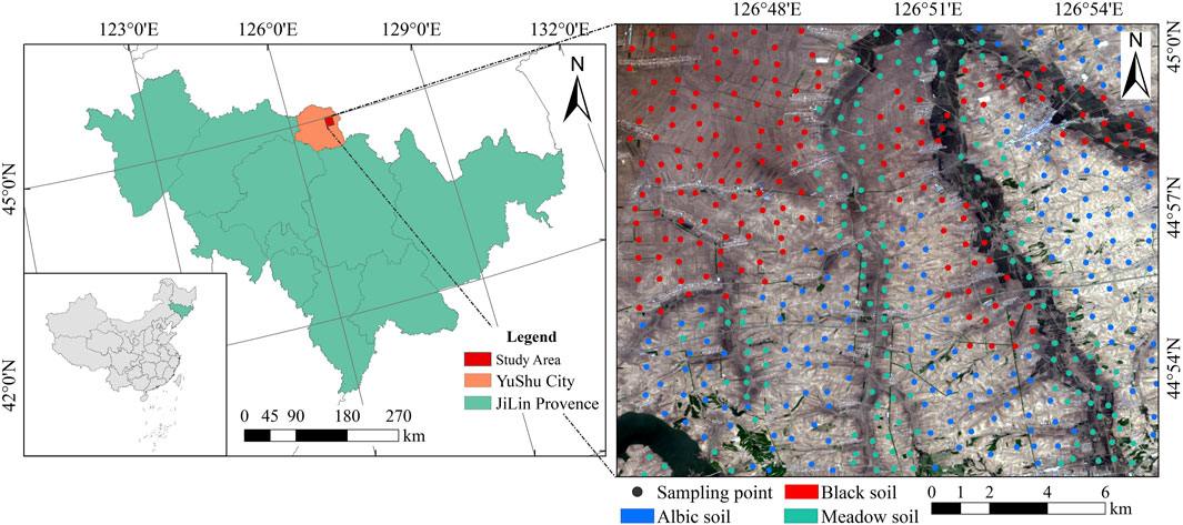
Figure 1. Map of the study area. The study area in Yushu City, Jilin Province, Northeast China and the soil types and sampling points distribution.
The soil samples were collected in late April 2022. At this time, the area was in the ‘bare soil phase’ without weeds and straw on the surface. The soil sampling points were set up referencing Chinese soil classification standards and combined with high-resolution remote sensing imagery of the study area. Through field investigation, the preset positions and collection route of sampling points were adjusted according to the soil surface heterogeneity in the area, thus ensuring that the sampling points were evenly distributed in the study area, and 502 soil samples were collected according to the sampling plan. To eliminate the influence of mixed pixels at sampling points on subsequent research, the spacing between sampling points with surrounding objects exceeded 100 m. The locations of the sampling points are shown in Figure 1. Soil samples were collected using the five-point sampling method to avoid accidental factors affecting the soil nutrient test results and to ensure the accuracy of the test. Firstly, a square area (30 × 30 m) was established at the sampling points, then 200 g of soil with a depth of 20 cm was collected at five points (four corner points and the center point), and the larger stones and debris were removed from the samples, which were finally mixed homogeneously and packed into sample bag. After sampling was completed, the serial number of sample points was set according to location and sampling sequence, and the global positioning system (GPS) was used to record the spatial coordinates, acquisition time and altitude of the center point. While soil samples were collected, the thickness of the black soil layer at each of the five sample points was measured and recorded by drilling and sampling method.
After sample collection, the soil samples were air-dried indoors, and non-soil bodies such as stones, weed roots, and straw were removed. Then, each soil sample was crushed with ceramic tools and sieved using a 100-mesh sieve with a particle size of 0.15 mm. The processed soil samples were divided into two parts for chemical analysis and spectral reflectance measurement (Figure 2). In this study, the spectral reflectance of soil samples was measured by an ASD FieldSpec 4 spectrometer. In order to avoid the influence of light sources and improve the measurement accuracy, sample measurement was performed in the darkroom, and the average of ten spectral reflectances was used as the measured spectral data of the soil samples. The content of TN in soil samples was determined by the semi-micro Kjeldahl method. The measuring process strictly follows the specification of land quality geochemical assessment in China.
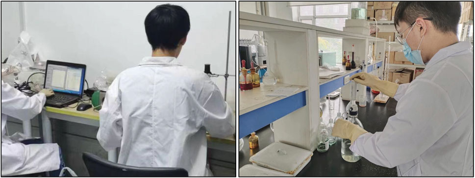
Figure 2. Soil Sample Pretreatment. Indoor spectral measurement of soil samples and determination of TN content in soil samples.
This study considers the synchronization of remote sensing imagery generation time with ground testing. According to the sampling time, the ZY1-02D satellite hyperspectral image generated on 26 April 2022 was selected as the spectral data source. The data were provided by the China Center for Resources Satellite Data and Applications. The ZY1-02D satellite is the first civilian hyperspectral operational satellite launched by the Ministry of Natural Resources of China. It is equipped with a visible near-infrared camera for simultaneous acquisition of panchromatic and multispectral data, and a hyperspectral camera with hyperspectral data in 166 bands (Yu et al., 2021). The visible and near-infrared (VNIR) has a spectral resolution of 10 nm and 76 bands in the spectral range. The short-wave infrared (SWIR) has a spectral resolution of 20 nm and 90 bands in the spectral range. In addition, the satellite can acquire high-precision geometric and radiometric information while receiving spectral information. It firstly achieves in-orbit yaw calibration of hyperspectral loads, facilitating applications such as quantitative inversion of crop nutrient content (Lu et al., 2021). Table 1 shows the parameter information of the ZY1-02D AHSI sensor. The topographic data used in this study are Digital Elevation Model (DEM) data from the United States Geological Survey (https://glovis.usgs.gov/) with a spatial resolution of 30 m.
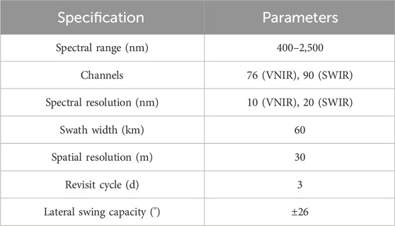
Table 1. Parameters of the ZY1-02D AHSI sensor.
To effectively estimate soil TN content in a wide range, three different grouping strategies were proposed for local regression estimation according to the differences in soil types, black soil layer thickness, and slope gradient in the study area. Afterward, the optimal grouping strategy was selected for estimating soil TN content. The following steps are mainly involved in estimation: data acquisition and processing, sample grouping and feature selection, TN content estimation model construction, and spatial distribution mapping (Figure 3). Firstly, the TN content in the soil samples was measured, and the soil type and black soil layer thickness at sampling points were statistically analyzed. Spectral curves and terrain parameters for each sample were extracted by preprocessing hyperspectral images and topographic data. Then, the spectral data were mathematically transformed, and the sensitive bands of each transformed spectrum for soil TN were screened based on the Pearson correlation coefficient threshold. In this way, the optimal spectral transformation method was determined. Furthermore, the local regression strategy for grouping soil samples was determined, and CARS was employed to extract the characteristic spectral bands of TN content for each group in different grouping strategies. Finally, the soil TN content estimation model was developed using the CatBoost algorithm, and the optimal grouping strategy was selected to estimate the soil TN content and plot the soil TN content distribution map.

Figure 3. Workflow for soil TN content estimation.
Aiming at the fringe phenomenon is obvious in the SWIR band data of the ZY1-02D hyperspectral camera, the “global de-stripe” method was used to repair the fringe, and the bands with serious water vapor interference and overlapping bands were eliminated. Finally, 400–1,341 nm, 1,459–1795 nm and 1963–2,470 nm were selected as the spectral bands for this experiment, with a total of 145 spectral channels. Based on the ENVI software platform, The ZY1-02D hyperspectral image of the investigated area was subjected to geometric correction, radiometric calibration and atmospheric correction to reduce or eliminate image quality degradation due to radiance distortion, atmospheric extinction and geometric distortion, and to obtain original reflectance data (Li et al., 2022). Then, eight different transformations were performed on the processed hyperspectral images to reduce the errors caused by noise, environment and other factors, and to enhance the spectral feature information, to extract the sensitive spectral bands of soil TN more accurately (Yumiti and Wang, 2022). These transformation methods include First Derivative Reflectance (FDR), Continuum Removal (CR), Logarithm Reflectance (log R), Recipro-cal logarithmic Reflectance [log(1/R)], Second Derivative Reflectance (SDR), Multiplicative Scatter Correction Reflectance (MSC-R), Standard Normal Variable Reflectance (SNV-R) and Detrend Reflectance (DT-R) (Gao et al., 2014; Chen et al., 2017).
After obtaining the DEM data from USGS, the DEM data of the test area were processed to fill in missing data, remove noise points and data smoothing, and the model was evaluated and calibrated according to the measured elevation values of each sample point, to ensure that the quality and accuracy of the DEM data meet the experimental requirements. Then, six topographic parameters including elevation, slope, aspect, longitudinal curvature (LC), cross-sectional curvature (CC) and surface roughness (SR) were extracted from the DEM data (Taghizadeh-Mehrjardi et al., 2014).
Hyperspectral data have many spectral bands and high dimensions, and the obvious multicollinearity between adjacent bands, which will affect the stability of the estimation model to some extent. Therefore, extracting appropriate spectral feature bands as input variables for model construction can effectively reduce or eliminate problems such as low model accuracy and slow speed caused by redundant bands. CARS is a feature variable selection algorithm based on iterative statistical information proposed by drawing on the “survival of the fittest” rule of Darwin’s evolutionary theory (Li et al., 2009). The algorithm selects the optimal set of variables by dynamically adjusting the window width and threshold, ensuring continuity of effective information. It has two stages of feature fast elimination and feature selection, which can effectively reduce the computation time and improve the prediction performance of the model (Zhao et al., 2022). It works on the following principle: (1) Monte Carlo iteration and competition are used to select multiple subsets from multicomponent spectral data. (2) The key wavelengths are selected by the key wavelengths are selected by exponential attenuation function and adaptive reweighted sampling (ARS). (3) Multiple rounds of cross-validation (CV) are used to select the variable subset with the minimum root mean square error validation (RMSEV) result (Zheng et al., 2012).
The CatBoost algorithm is an integrated learning predictive model with few parameters, high accuracy and support for categorical features that extensions and improvements on the Gradient Boosting Decision Tree (GBDT) algorithm (Hancock and Khoshgoftaar, 2020). Unlike the traditional GBDT algorithm, the algorithm randomly sorts all samples and then calculates the average labeled value for that sample, and the same category value placed before the given category value (Wang WC. et al., 2022). In addition, the algorithm improves Greedy Target-based Statistics by adding prior distribution terms, which can effectively reduce the noise caused by low-frequency categorical data. Suppose a permutation is
where
Compared with other ensemble learning algorithms, CatBoost has the following characteristics: (1) It uses a combination of category features, which enriches the feature dimensions by exploiting the linkage between the features. (2) It uses sort boosting to counteract the noisy points in the training set, thus avoiding the bias of gradient estimation, and then solving the problem of prediction bias, which leads to a significant increase in the speed of model training speed and accuracy. (3) It uses oblivious trees as the base model, which makes the model better able to deal with the high-dimensional sparse data (Huang et al., 2019). Table 2 shows the main parameters of the CatBoost algorithm and the search range of Bayesian optimization.
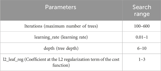
Table 2. The main training parameters and range of the CatBoost algorithm.
To assess the stability and estimation performance of the model, three statistical parameters are calculated as the accuracy evaluation index of the model: coefficient of determination (
where
This study statistically analyzed the TN content of the collected soil samples, as shown in Table 3. The TN content of the sample set in the experimental area ranged from 0.55 g/kg to 2.34 g/kg, with a mean value (Mean) of 1.31 g/kg and a coefficient of variation (CV) of 20.61%. Among the different soil types in the study area, the meadow soil had the highest TN content (mean = 1.42 g/kg), and the albic soil had the lowest TN content (mean = 1.21 g/kg) and the highest CV (CV = 24.79%). In addition, the CVs for all three soil types were higher than those for the entire sample, indicating that dividing the sample set by soil type increased the spatial variability of sample TN content.
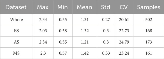
Table 3. Descriptive statistics of TN content in soil samples (Unit: g/kg).
In order to explore the influence of terrain heterogeneity on the estimation accuracy of TN content, the correlation between soil TN content and several topographic factors (e.g., elevation, slope, and aspect) was analyzed in this study. The topographic factor exhibiting the highest correlation was selected as the partitioned data for local regression. The Pearson correlation coefficients between soil TN content and topographic factors are shown in Table 4. Because the slope had the highest correlation with soil TN content among different topographic factors, it was selected as the segmentation data for local regression estimation. To clarify the variation in the TN content distribution with different slopes and thicknesses of the black soil layer, the soil samples were divided according to the slope grade and the thickness of the soil black soil layer. The distribution of the soil TN content was plotted, as shown in Figure 4. Most of the study area has a slope of 0–3°. With increasing slope, the proportion of samples with soil TN content of 0–1 g/kg increases, and the proportion of samples with TN content of >1.5 g/kg decreases. In Figure 4, 83.66% of the samples have a black soil layer thickness between 0 cm and 60 cm. As the thickness of the black soil layer increases, the proportion of samples with soil TN content of >1.5 g/kg increases, and that of samples with soil TN content between 0 and 1 g/kg and one–1.5 g/kg decreases to varying degrees.

Table 4. Pearson correlation between TN and topographic factors.
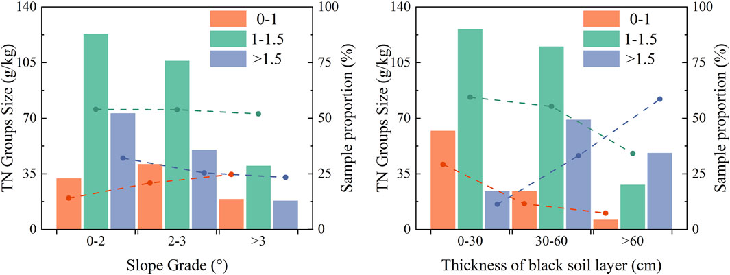
Figure 4. Spatial distribution of TN content.
To determine the optimal local regression strategy for estimating soil TN content, all soil samples were grouped according to different strategies. The grouping results of the three strategies are shown in Table 5: (1) grouping by soil type (ST-G): All samples were classified into three groups according to the soil subtypes of albic soil (AS), meadow soil (MS), and black soil (BS); (2) grouping by the thickness of black soil layer (BLT-G): According to the thickness of the black soil layer, the number of sample sets, and the distribution range of TN content, all soil samples were divided into three groups, namely, BLT1 (0–30 cm), BLT2 (30–60 cm), and BLT3 (>60 cm); (3) Grouping by slope grade (Slp-G): Based on the slope values of the soil samples, the number of subsample sets, and the distribution range of soil TN content, all samples were divided into three groups, namely, Slp1 (0°–2°), Slp2 (2°–3°), and Slp3 (>3°).
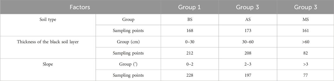
Table 5. Analysis of grouping results.
To verify the feasibility of soil TN content estimation after ZY1-02D hyperspectral image correction, the measured spectra of 502 samples were resampled following the spectral resolution of the hyperspectral image. The spectral curves of the resampled spectra were compared with those of the image pixels (Figure 5). It can be seen that the spectral reflectances of the image pixels are lower than the measured soil spectral reflectances, which can be attributed to factors such as soil water content and soil surface roughness. However, the spectral curves of the image pixels and the measured spectral curves have similar characteristic absorption positions, and the shapes and trends of the two curves are highly consistent, validating the reliability of preprocessing, such as radiometric calibration and atmospheric correction. A high correlation can be observed with the correlation coefficients ranging from 0.6 to 0.84 for the entire band, indicating that most of the soil spectral features are retained in the image pixels. These features can be used to estimate soil components and physicochemical information. In addition, the measured spectra and image pixel spectra of all samples were classified into five groups according to the TN content from low to high. The spectral data and the corresponding content data of each group were averaged for comparison and analysis, as shown in Figure 5. In the wavelength range of 400–2,500 nm, the spectral reflectance decreases with increasing soil TN content, and the patterns of the image pixel spectra and the measured spectra with the soil TN content are generally consistent, further proving the feasibility of using the ZY1-02D hyperspectral image for soil TN content estimation.
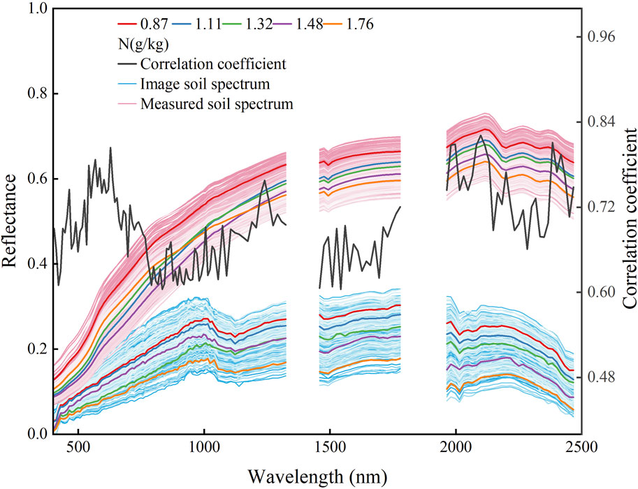
Figure 5. Image and measured soil spectrum, and correlation coefficients.
With the aim of reducing the interference of other factors (e.g., noise and environment) and enhancing the spectral feature information for more accurate identification of the sensitive bands of soil TN, eight different transformations were applied to the raw reflectance data, including FDR, CR, log R, log(1/R), SDR, MSC-R, SNV-R, and DT-R transformations. As shown in Figure 6, the reflectance and absorption characteristics of the spectral curves are substantially increased with more peak and trough information after spectral transformation, and more sensitive spectral bands can be identified.
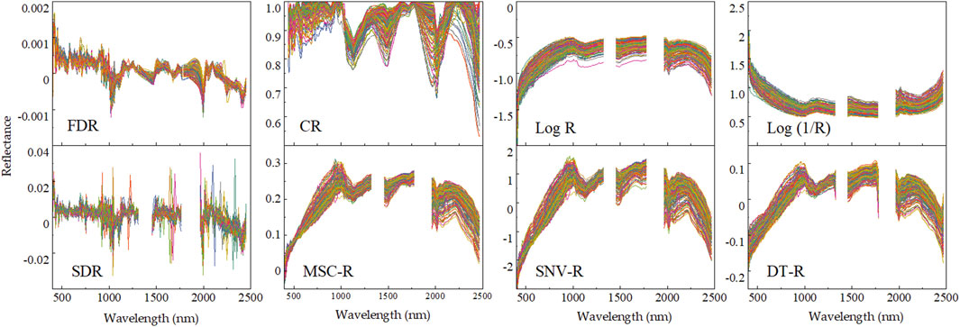
Figure 6. Transformation spectral reflectance curves.
To determine the optimal spectral transformation method for estimating TN content, this study was based on three sample grouping strategies, and the original spectral reflectance and eight transformed spectral reflectances of each soil sample group were correlated with their TN content. Figure 7 reveals a negative correlation between OR and soil TN content in the wavelength range of 400–2,500 nm. In most wavelength ranges, the soil TN content exhibits a markedly higher correlation coefficient with the transformed spectral reflectance than with the original reflectance. The bands with an absolute correlation coefficient greater than 0.5 were selected as the sensitive bands, and the number of sensitive bands of each group of soil samples under different transformation methods was counted. As shown in Table 6, there are significant differences in the number of TN sensitive bands in each sample group under different transformation methods, and the number of sensitive bands after FDR and CR transformation increases significantly. Among them, the number of sensitive bands in the FDR spectra is the highest, except for the “BLT1 (0–30 cm)” group. Based on the above results, the first derivative method was selected to transform the soil spectral characteristics.
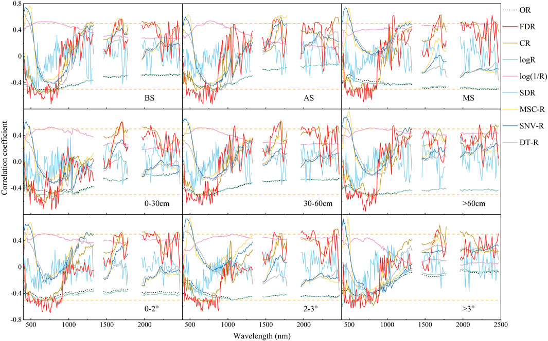
Figure 7. Correlation between soil TN content and the spectral reflectance of each band.
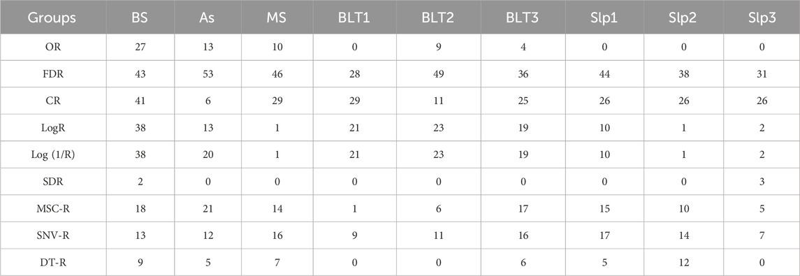
Table 6. Number of sensitive bands of different spectral transformation methods.
To obtain the set of spectral feature variables with minimum redundancy information and to improve the efficiency and accuracy of the estimation model, the CARS algorithm was applied to choose the best spectrum variables of the sample set. In the CARS feature selection process, the number of Monte Carlo iterations was set to 50. After multiple iterations, the cross-validation RMSE (RMSECV) values of each band combination scheme were compared, and the variable set corresponding to the minimum RMSECV value was selected as the optimal variable set for the model. Figure 8 shows the optimal variable set plots for each sample set divided according to different factors. By analyzing the optimal number of variables in all sample sets, the number of bands selected accounts for 11%–15% of the total number of bands, significantly reducing redundant information. Furthermore, most of the characteristic wavelengths selected using the whole sample as input data are concentrated in the range of 550–850 nm. After grouping the samples according to different factors, each grouping strategy corresponded to a wider distribution of characteristic wavelengths, with the ST-G strategy corresponding to the widest distribution of characteristic wavelengths. Combining the optimal results of the whole sample and each sub-sample, the characteristic wavelengths were mainly concentrated in the ranges of 450–850 nm, 1950–2,150 nm, and 2,400–2,450 nm, with a relative concentration in the range of 550–850 nm. Figure 9 shows the CARS variable selection process with the ST-G strategy (BS, AS, and MS), and the variable set with the lowest RMSECV value is marked by a vertical line. The 1st-22nd iterations are the rough selection phase of the CARS selection feature, and the wavelengths containing noise and useless information are quickly eliminated. As the number of iterations increases, the number of variables decreases exponentially. The 23rd to 50th iterations are the accurate selection stage of the CARS selection features. Starting from the 22nd iteration, the RMSECV of the three sample sets gradually reaches the lowest value and then increases, which can be attributed to the elimination of key bands sensitive to TN, resulting in lower model accuracy. After the 44th iteration, the RMSECV values gradually stabilized. The RMSECV values for BS, AS, and MS reach their minimum at the 22nd, 23rd, and 25th iterations, with 21, 19, and 17 retained wavelengths, respectively.
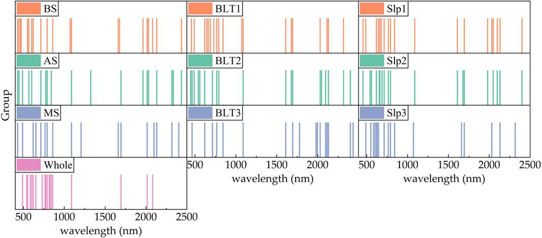
Figure 8. Optimal variable set graph (Horizontal coordinates indicate wavelengths from 400–2,500 nm, and vertical coordinates indicate different groups based on the ST-G, Slp-G, and BLT-G strategies).
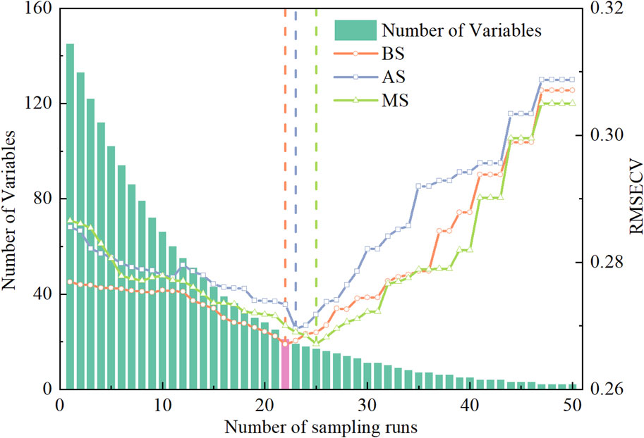
Figure 9. Variable selecting process with CARS (taking BS, AS, and MS as examples).
To clarify the influence of local regression according to different grouping strategies on the accuracy of TN content estimation, the CatBoost algorithm was used to perform local regression estimation on ST-G, BLT-G, and Slp-G strategies. The global regression estimation was also conducted based on the full sample (U-G strategy). The FDR data selected by CARS were used as the independent variable
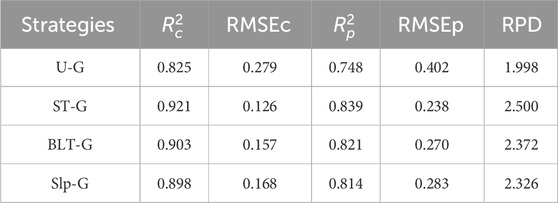
Table 7. Estimation accuracy index of different grouping strategies.
To verify the effectiveness of local regression in improving the estimation accuracy, this study further analyzed the estimation accuracy of each subgroup based on the CatBoost algorithm, as shown in Figure 10. Estimation accuracies for samples divided according to soil environment differences are higher than those for the whole sample. When adopting the BLT-G and Slp-G strategies for regression estimation, a large difference in estimation accuracy between groups can be observed, and the estimation results easily fall into the local optimum. The difference in estimation accuracy between groups classified with the ST-G strategy is the smallest, and the
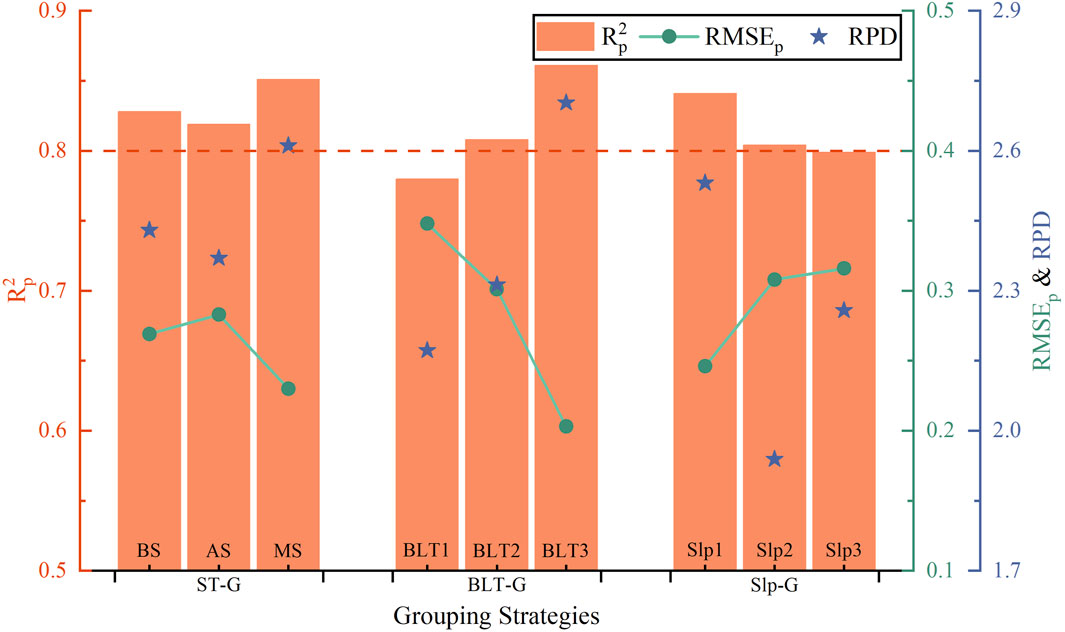
Figure 10. Accuracy of TN content estimation for each subgroup under different grouping strategies.
To improve the accuracy of TN content estimation and mapping in the study area, the ZY1-02D satellite remote sensing image was used as the data source, the training samples were determined by the region of interest, and the SVM algorithm was used to supervise the classification of hyperspectral images and extract farmland pixels. Figure 11A shows the selection results of the farmland pixels, with approximately 83% of the study area being farmland, the selected farmland soil ranges have clear boundaries with non-farmland pixels (e.g., roads and construction land) and relatively intact patches. It can be seen from Table 7 and Figure 10 that the local regression estimation model constructed according to the ST-G strategy has high estimation accuracy and stability. Therefore, we divided the farmland pixels in the experimental area into three sub-regions according to different soil types, and the TN content of the three sub-regions was mapped using the CatBoost algorithm, and the spatial distribution map of soil TN content in the whole study area was obtained by mosaic and merging. As shown in Figure 11B, the TN content of the cultivated soils in the study area is generally high, mainly concentrated in the range of 1.0–2.0 g/kg. The soil area in the range of 1.0–1.5 g/kg accounts for 37.49% of the farmland area (Figure 11C). The soil area in the range of 1.5–2.0 g/kg accounts for the largest proportion (57.75% of the farmland area) and is evenly distributed throughout the study area (Figure 11D). The spatial distribution of soil TN content was characterized by obvious clustering, with the distribution of high- and low-value areas relatively concentrated. The high-value areas are zonally distributed in the eastern part of the study area (Figure 11E), which is due to the paddy field in this part, where the long-term application of nitrogen fertilizer and irrigation results in high humus content, allowing for the transformation and accumulation of nitrogen in the soil. The low-value areas are mainly distributed in the southern part of the study area (Figure 11B), where the undulating topography leads to soil erosion and lower nitrogen retention. Compared with the high spatial resolution image maps for the study area, we can observe that the estimation result of soil TN content has a high coincidence with the current status of farmland cultivation in the study area, demonstrating the reliability of the local regression estimation model based on the ST-G strategy and Cat Boost algorithm.
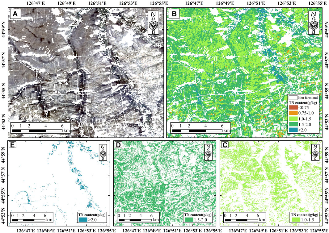
Figure 11. Mapping of soil TN content for the study area. (A) Farmland pixel extraction results, (B–E) Spatial distribution of TN content.
To clarify the degree of accuracy improvement in the TN content estimation by local regression according to different grouping strategies and to verify the superiority of the CatBoost algorithm for local regression estimation, a comparative analysis was conducted using different algorithms and grouping strategies. The scatter plots of estimated and measured TN content with different grouping strategies and estimation algorithms are shown in Figure 12. For the CatBoost algorithm, the ST-G strategy has the best fitting effect and the highest estimation accuracy, followed by the BLT-G strategy. The
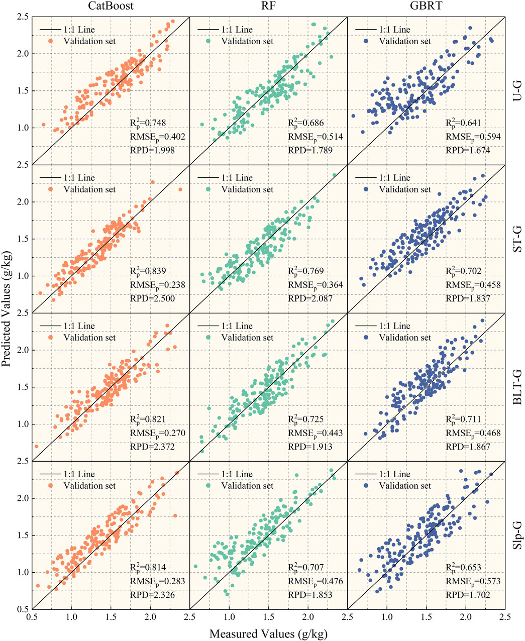
Figure 12. Scatter plots of the estimated and measured TN content with different grouping strategies and estimation models.
In this study, eight transformation methods (e.g., FDR, CR, and SNV-R) were used to spectrally transform the original spectrum, and the distribution of TN characteristic bands was determined by the correlation between each transformed spectrum and soil TN content (Figure 7). The characteristic bands of the CR transform are mainly distributed around 700–850 nm, 1700 nm, and 2,400 nm, and those of the FDR transform are mainly distributed in ranges of 450–850 nm, 1,650–1750 nm, and 1950–2,150 nm. Furthermore, the MSC-R transform and SNV-R transform show a similar distribution of the characteristic bands near 500 nm. The above results are consistent with previous findings (Shen et al., 2020; Vibhute et al., 2020; Liu et al., 2023; Zhang RR. et al., 2023). However, not all spectral transformations produce results superior to the original reflectance (Xie et al., 2022). The SDR transform has few characteristic band distributions over the full band range. In this study, the subset of samples for local regression estimation was divided according to differences in soil type, slope, and thickness of the black soil layer. The TN content data and FDR spectral reflectance data of different sample sets were used as input data, and the characteristic bands of each sample set were selected by CARS. According to the results of CARS feature selection (Figure 8), the TN characteristic bands selected using the whole sample as input data were mainly distributed in the rages of 550–650 nm and 750–850 nm, and some selected wavelengths are consistent with the previous studies (Kawamura et al., 2017; Shen et al., 2020).
When the samples were divided based on different environmental factors for local regression estimation, some differences appeared in the characteristic bands corresponding to the sample sets with different data characteristics. Therefore, to clarify the distribution of TN characteristic bands corresponding to the sample subset, the correlation between the soil TN content and the FDR data was examined in this study, and the spectral bands with the absolute Pearson correlation coefficient greater than 0.5 were used as the characteristic bands. The TN characteristic bands of different sample sets are shown in Figure 13. It can be seen that characteristic bands based on the whole sample are mainly distributed in the range of 450–850 nm. After dividing samples according to different grouping strategies, the number and distribution range of the characteristic bands are more abundant. When using the ST-G strategy, characteristic bands show wider distribution ranges, mainly in 450–850 nm, 1,600–1750 nm, and 1950–2,150 nm. When using the Slp-G strategy, the number of characteristic bands of three sample sets increases (the added characteristic bands are mainly distributed in the range of 1950–2,150 nm and 2,300–2,450 nm). After grouping with the BLT-G strategy, the variation of the soil TN characteristic bands is more significant, with increasing characteristic spectral bands in the ranges of 1,600–1750 nm and 1950–2,450 nm as the thickness increases. Therefore, more abundant spectral information can be obtained for the data characteristics of various sample sets after dividing samples with different strategies. It is the key reason for the improved accuracy of local regression estimation.
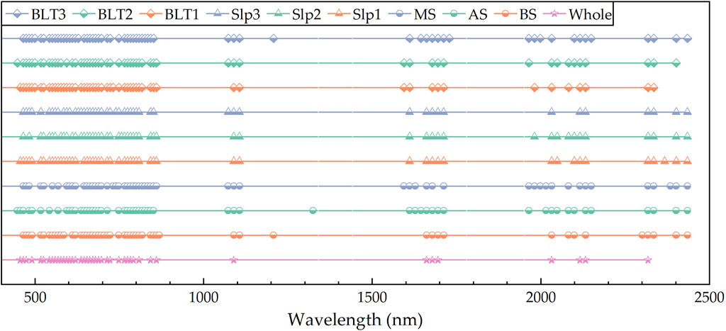
Figure 13. Distribution of TN characteristic bands for different sample sets (The vertical coordinates represent the whole sample and the different sample sets divided according to the set grouping strategy).
When mapping the distribution of soil TN content based on hyperspectral images, the accuracy of estimation and mapping is influenced by potential factors such as the imaging endmember spectra, the laboratory measurement process, and geographic environmental differences. During hyperspectral image acquisition, differences in radiation intensity and meteorological conditions can result in different endmember spectral reflections, thus affecting the accuracy of estimation and mapping (Li XP. et al., 2019). In this study, we ensure that the sampling time of the soil samples is consistent with the satellite detection time, the sampling points are within the pure bare soil pixels, and strict image preprocessing is performed to reduce the influence of spectral information. In addition, the soil samples used in this study were measured under the same environments, and the influence of the laboratory measurement process can be ignored. The difference in geographical environment will alter the soil nitrogen content and its distribution to different degrees, thus affecting the accuracy of TN content estimation (Zhong et al., 2019; Wang et al., 2021; Dai et al., 2022). Aiming at the influence of soil environmental factors on the estimation accuracy, a local regression estimation model based on sample grouping was established, which weakens the differences in soil TN content among regions, thus reducing the influence of soil environmental heterogeneity on model training and estimation, and effectively improving the estimation accuracy of soil TN content.
Because soils exist in relatively complex environments over long periods, the distribution of soil nitrogen is influenced by the coupling of various soil environmental factors such as slope, elevation, and the thickness of the black soil layer. Restricted by the number of sampling points and the sample distribution density, this study establishes a local regression model to estimate soil TN content based on the difference of a single environmental factor, which has the problems of low inversion accuracy and poor transferability. Sample splitting by considering multiple factors at the same time can result in an insufficient number of samples, abruptly increasing the modeling difficulty and even reducing the estimation accuracy of soil TN content. Therefore, future research will attempt to increase the sampling density, supplement sample sets, introduce more soil environmental information, and thoroughly analyze the relationship between multiple soil environmental factors and soil nitrogen distribution, and establish a soil TN content estimation model that considers the heterogeneity of multiple environmental factors. Through these attempts, the accuracy and transferability of the estimation model will be strengthened, thus facilitating the rapid and large-scale estimation of soil TN content.
When hyperspectral remote sensing images are used to construct a model for estimating soil TN content, the accuracy of the model is influenced by image quality and sample characteristics. In this study, based on ZY1-02D hyperspectral remote sensing image and soil environmental data, we constructed a local regression estimation model of nitrogen content taking into account the heterogeneity of soil environment, which effectively improved the accuracy and stability of the soil TN content estimation model. After analyzing the correlation between soil TN content and environmental parameters, three strategies for grouping soil samples were established by dividing the samples according to differences in soil types, thicknesses of the black soil layer, and slope grade, which effectively highlight the characteristic information of each sample subset, weaken the influence of soil TN content difference between regions on the accuracy of the estimation model, and reduce the possibility that the accuracy of the estimation model falling into the local optimum due to soil environmental heterogeneity. In the study, the optimal wavelength variables for local regression according to the data characteristics of each sample subset, which enrich the spectral feature information of the modeled samples, and effectively solve the problems of poor generalization ability and poor robustness faced by the traditional global regression estimation model. By comparing the accuracy indices of each estimation model, the estimation performance of the local regression model constructed according to the ST-G strategy and the CatBoost algorithm is better than that of the global regression model and other local regression models, with a validation set RMSE of 0.238 and
The original contributions presented in the study are included in the article/Supplementary Material, further inquiries can be directed to the corresponding author.
NL: Conceptualization, Data curation, Formal Analysis, Funding acquisition, Investigation, Project administration, Resources, Supervision, Validation, Writing–original draft, Writing–review and editing. XM: Visualization, Writing–original draft, Writing–review and editing. JL: Data curation, Resources, Writing–original draft. RJ: Resources, Software, Validation, Writing–original draft. MW: Data curation, Investigation, Resources, Writing–original draft. WZ: Validation, Writing–original draft, Formal Analysis.
The author(s) declare that financial support was received for the research, authorship, and/or publication of this article. This research was funded by the Science and Technology Development Project of Jilin Province (20210203016SF), the Natural Science Foundation of Jilin Province (20230101373JC), the National Natural Science Foundation of China (52178042), and the Key Scientific Research Project of the Education Department of Jilin Province (JJKH20200280KJ).
The authors would like to thank the China Centre for Resources Satellite Data and Application for providing ZY1-02D data. We are most grateful to the reviewers and editors for their valuable comments and recommendations.
The authors declare that the research was conducted in the absence of any commercial or financial relationships that could be construed as a potential conflict of interest.
All claims expressed in this article are solely those of the authors and do not necessarily represent those of their affiliated organizations, or those of the publisher, the editors and the reviewers. Any product that may be evaluated in this article, or claim that may be made by its manufacturer, is not guaranteed or endorsed by the publisher.
The Supplementary Material for this article can be found online at: https://www.frontiersin.org/articles/10.3389/fenvs.2024.1401107/full#supplementary-material
Chatterjee, S., Hartemink, A. E., Triantafilis, J., Desai, A. R., Soldat, D., Zhu, J., et al. (2021). Characterization of field-scale soil variation using a stepwise multi-sensor fusion approach and a cost-benefit analysis. Catena 201, 105190. doi:10.1016/j.catena.2021.105190
Chen, Y. Y., Zhao, R. Y., Qi, T. C., Qi, L., and Zhang, C. (2017). Constructing representative calibration dataset based on spectral transformation and kennard-stone algorithm for VNIR modeling of soil total nitrogen in paddy soil. Spectrosc. Spectr. Analysis 37 (7), 2133–2139. doi:10.3964/j.issn.1000-0593(2017)07-2133-07
Cheng, H., Wang, J., and Du, Y. K. (2021). Combining multivariate method and spectral variable selection for soil total nitrogen estimation by Vis-NIR spectroscopy. Archives Agron. Soil Sci. 67 (12), 1665–1678. doi:10.1080/03650340.2020.1802013
Dai, L. J., Ge, J. S., Wang, L. Q., Zhang, Q., Liang, T., Bolan, N., et al. (2022). Influence of soil properties, topography, and land cover on soil organic carbon and total nitrogen concentration: a case study in Qinghai-Tibet plateau based on random forest regression and structural equation modeling. Sci. Total Environ. 821, 153440. doi:10.1016/j.scitotenv.2022.153440
Deng, X. F., Ma, W. Z., Ren, Z. Q., Zhang, M. H., Grieneisen, M. L., Chen, X. J., et al. (2020). Spatial and temporal trends of soil total nitrogen and C/N ratio for croplands of East China. Geoderma 361, 114035. doi:10.1016/j.geoderma.2019.114035
Du, C. W., and Zhou, J. M. (2009). Evaluation of soil fertility using infrared spectroscopy: a review. Environ. Chem. Lett. 7 (2), 97–113. doi:10.1007/s10311-008-0166-x
Gao, X. H., Yang, Y., Zhang, W., Jia, W., Li, J. S., Tian, C. M., et al. (2014). “Visible-near infrared reflectance spectroscopy for estimating soil total nitrogen contents in the Sanjiang Yuan Regions, China -A case study of Yushu county and Maduo county,Qinghai province”, in Multispectral, Hyperspectral, and Ultraspectral Remote Sensing Technology, Techniques and Applications V. (Beijing, China: Spie-Int Soc Optical Engineering), Vol. 9263, 295–306. doi:10.1117/12.2069107
Ge, N. N., Wei, X. R., Wang, X., Liu, X. T., Shao, M. A., Jia, X. X., et al. (2019). Soil texture determines the distribution of aggregate-associated carbon, nitrogen and phosphorous under two contrasting land use types in the Loess Plateau. Catena 172, 148–157. doi:10.1016/j.catena.2018.08.021
Grunwald, S., Vasques, G. M., and Rivero, R. G. (2015). Advances in agronomy. Delaware, United States: University of Delaware, Newark.
Gu, Z. J., Xie, Y., Gao, Y., Ren, X. Y., Cheng, C. C., and Wang, S. C. (2018). Quantitative assessment of soil productivity and predicted impacts of water erosion in the black soil region of northeastern China. Sci. Total Environ. 637, 706–716. doi:10.1016/j.scitotenv.2018.05.061
Guo, P., Li, T., Gao, H., Chen, X. W., Cui, Y. F., and Huang, Y. R. (2021). Evaluating calibration and spectral variable selection methods for predicting three soil nutrients using vis-NIR spectroscopy. Remote Sens. 13 (19), 4000. doi:10.3390/rs13194000
Hancock, J. T., and Khoshgoftaar, T. M. (2020). CatBoost for big data: an interdisciplinary review. J. Big Data 7 (1), 94. doi:10.1186/s40537-020-00369-8
Hong, Y. S., Liu, Y., Chen, Y. Y., Liu, Y. F., Yu, L., Liu, Y., et al. (2019). Application of fractional-order derivative in the quantitative estimation of soil organic matter content through visible and near-infrared spectroscopy. Geoderma 337, 758–769. doi:10.1016/j.geoderma.2018.10.025
Huang, G. M., Wu, L. F., Ma, X., Zhang, W. Q., Fan, J. L., Yu, X., et al. (2019). Evaluation of CatBoost method for prediction of reference evapotranspiration in humid regions. J. Hydrology 574, 1029–1041. doi:10.1016/j.jhydrol.2019.04.085
Jia, S. Y., Li, H. Y., Wang, Y. J., Tong, R. Y., and Li, Q. (2017). Hyperspectral imaging analysis for the classification of soil types and the determination of soil total nitrogen. Sensors 17 (10), 2252. doi:10.3390/s17102252
Jiang, C. L., Zhao, J. Y., Ding, Y. Y., and Li, G. R. (2023a). Vis-NIR spectroscopy combined with gan data augmentation for predicting soil nutrients in degraded alpine meadows on the qinghai-tibet plateau. Sensors 23 (7), 3686. doi:10.3390/s23073686
Jiang, C. L., Zhao, J. Y., and Li, G. R. (2023b). Integration of vis-NIR spectroscopy and machine learning techniques to predict eight soil parameters in alpine regions. Agronomy-Basel 13 (11), 2816. doi:10.3390/agronomy13112816
Kawamura, K., Tsujimoto, Y., Rabenarivo, M., Asai, H., Andriamananjara, A., and Rakotoson, T. (2017). Vis-NIR spectroscopy and PLS regression with waveband selection for estimating the total C and N of paddy soils in Madagascar. Remote Sens. 9 (10), 1081. doi:10.3390/rs9101081
Li, H., Wang, J., Zhang, J., Liu, T., Acquah, G. E., and Yuan, H. (2022). Combining variable selection and multiple linear regression for soil organic matter and total nitrogen estimation by DRIFT-MIR spectroscopy. Agronomy-Basel 12 (3), 638. doi:10.3390/agronomy12030638
Li, H. D., Liang, Y. Z., Xu, Q. S., and Cao, D. S. (2009). Key wavelengths screening using competitive adaptive reweighted sampling method for multivariate calibration. Anal. Chim. Acta 648 (1), 77–84. doi:10.1016/j.aca.2009.06.046
Li, H. Y., Jia, S. Y., and Le, Z. C. (2019a). Quantitative analysis of soil total nitrogen using hyperspectral imaging Technology with extreme learning machine. Sensors 19 (20), 4355. doi:10.3390/s19204355
Li, X. P., Zhang, F., and Wang, X. P. (2019b). Study on differential-based multispectral modeling of soil organic matter in ebinur lake wetland. Spectrosc. Spectr. Analysis 39 (2), 535–542. doi:10.3964/j.issn.1000-0593(2019)02-0535-08
Li, X. Y., Fan, P. P., Liu, Y., Wang, Q., and Lü, M. R. (2019c). Extracting characteristic wavelength of soil nutrients based on multi-classifier fusion. Spectrosc. Spectr. Analysis 39 (9), 2862–2867. doi:10.3964/j.issn.1000-0593(2019)09-2862-06
Liu, K., Wang, Y. F., Wang, X. D., Sun, Z. P., Song, Y. H., Di, H. G., et al. (2023). Characteristic bands extraction method and prediction of soil nutrient contents based on an analytic hierarchy process. Measurement 220, 113408. doi:10.1016/j.measurement.2023.113408
Liu, Z. F., Lei, H. C., Lei, L., and Sheng, H. Y. (2022). Spatial prediction of total nitrogen in soil surface layer based on machine learning. Sustainability 14 (19), 11998. doi:10.3390/su141911998
Lori, M., Symanczik, S., Maeder, P., Efosa, N., Jaenicke, S., Buegger, F., et al. (2018). Distinct nitrogen provisioning from organic amendments in soil as influenced by farming system and water regime. Front. Environ. Sci. 6. doi:10.3389/fenvs.2018.00040
Lu, H., Qiao, D. Y., Li, Y. X., Wu, S., and Deng, L. (2021). Fusion of China ZY-1 02D hyperspectral data and multispectral data: which methods should Be used? Remote Sens. 13 (12), 2354. doi:10.3390/rs13122354
Marty, C., Houle, D., Gagnon, C., and Courchesne, F. (2017). The relationships of soil total nitrogen concentrations, pools and C:N ratios with climate, vegetation types and nitrate deposition in temperate and boreal forests of eastern Canada. Catena 152, 163–172. doi:10.1016/j.catena.2017.01.014
Mendes, W. D., Sommer, M., Koszinski, S., and Wehrhan, M. (2022). Peatlands spectral data influence in global spectral modelling of soil organic carbon and total nitrogen using visible-near-infrared spectroscopy. J. Environ. Manag. 317, 115383. doi:10.1016/j.jenvman.2022.115383
Minu, S., Shetty, A., and Gomez, C. (2018). Hybrid atmospheric correction algorithms and evaluation on VNIR/SWIR Hyperion satellite data for soil organic carbon prediction. Int. J. Remote Sens. 39 (22), 8246–8270. doi:10.1080/01431161.2018.1483087
Minu, S., Shetty, A., Minasny, B., and Gomez, C. (2017). The role of atmospheric correction algorithms in the prediction of soil organic carbon from Hyperion data. Int. J. Remote Sens. 38 (23), 6435–6456. doi:10.1080/01431161.2017.1354265
Niu, J. C., Tang, H. Z., Liu, Q., Cheng, F., Zhang, L. N., Sang, L. L., et al. (2022). Determinants of soil bacterial diversity in a black soil region in a large-scale area. Land 11 (5), 731. doi:10.3390/land11050731
Pan, Y., Zhang, X. L., Liu, H. J., Wu, D. Q., Dou, X., Xu, M. Y., et al. (2022). Remote sensing inversion of soil organic matter by using the subregion method at the field scale. Precis. Agric. 23 (5), 1813–1835. doi:10.1007/s11119-022-09914-2
Peng, Y. P., Wang, L., Zhao, L., Liu, Z. H., Lin, C. J., Hu, Y. M., et al. (2021). Estimation of soil nutrient content using hyperspectral data. Agriculture-Basel 11 (11), 1129. doi:10.3390/agriculture11111129
Peng, Y. P., Zhao, L., Hu, Y. M., Wang, G. X., Wang, L., and Liu, Z. H. (2019). Prediction of soil nutrient contents using visible and near-infrared reflectance spectroscopy. Isprs Int. J. Geo-Information 8 (10), 437. doi:10.3390/ijgi8100437
Pennock, D. J. (2005). Precision conservation for co-management of carbon and nitrogen on the Canadian prairies. J. Soil Water Conservation 60 (6), 396–401.
Shen, L. Z., Gao, M. F., Yan, J. W., Li, Z. L., Leng, P., Yang, Q., et al. (2020). Hyperspectral estimation of soil organic matter content using different spectral preprocessing techniques and PLSR method. Remote Sens. 12 (7), 1206. doi:10.3390/rs12071206
Sinfield, J. V., Fagerman, D., and Colic, O. (2010). Evaluation of sensing technologies for on-the-go detection of macro-nutrients in cultivated soils. Comput. Electron. Agric. 70 (1), 1–18. doi:10.1016/j.compag.2009.09.017
Stenberg, B., and Rossel, R. A. V. (2010). Diffuse reflectance spectroscopy for high-resolution soil sensing. Sydney, Australia: Univ Sydney Fac Agr, Food and Nat Resources.
Taghizadeh-Mehrjardi, R., Minasny, B., Sarmadian, F., and Malone, B. P. (2014). Digital mapping of soil salinity in Ardakan region, central Iran. Geoderma 213, 15–28. doi:10.1016/j.geoderma.2013.07.020
Tesfaye, M. A., Bravo, F., Ruiz-Peinado, R., Pando, V., and Bravo-Oviedo, A. (2016). Impact of changes in land use, species and elevation on soil organic carbon and total nitrogen in Ethiopian Central Highlands. Geoderma 261, 70–79. doi:10.1016/j.geoderma.2015.06.022
Van Waes, C., Mestdagh, I., Lootens, P., and Carlier, L. (2005). Possibilities of near infrared reflectance spectroscopy for the prediction of organic carbon concentrations in grassland soils. J. Agric. Sci. 143, 487–492. doi:10.1017/s0021859605005630
Vibhute, A. D., Kale, K. V., Gaikwad, S. V., and Dhumal, R. K. (2020). Estimation of soil nitrogen in agricultural regions by VNIR reflectance spectroscopy. Sn Appl. Sci. 2 (9), 1523. doi:10.1007/s42452-020-03322-9
Wang, J., Wang, Y., Wang, W., Shi, L., and Si, H. (2022a). Transfer-learning-based cloud detection for Zhuhai-1 satellite hyperspectral imagery. Front. Environ. Sci. 10. doi:10.3389/fenvs.2022.1039249
Wang, W. C., Yang, W., Zhou, P., Cui, Y. L., Wang, D., and Li, M. Z. (2022b). Development and performance test of a vehicle-mounted total nitrogen content prediction system based on the fusion of near-infrared spectroscopy and image information. Comput. Electron. Agric., 192, 106613. doi:10.1016/j.compag.2021.106613
Wang, Y., Xu, Y., Yang, H., Shen, H., Zhao, L., Zhu, B., et al. (2023). Effect of slope shape on soil aggregate stability of slope farmland in black soil region. Front. Environ. Sci. 11. doi:10.3389/fenvs.2023.1127043
Wang, Z. G., Wang, G. C., Zhang, G. H., Wang, H. B., and Ren, T. Y. (2021). Effects of land use types and environmental factors on spatial distribution of soil total nitrogen in a coalfield on the Loess Plateau, China. Soil and Tillage Res., 211, 105027. doi:10.1016/j.still.2021.105027
Wilding, L. P., and Lin, H. (2006). Advancing the frontiers of soil science towards a geoscience. Geoderma 131 (3-4), 257–274. doi:10.1016/j.geoderma.2005.03.028
Wu, L., Qiao, S. S., Peng, M., and Ma, X. Y. (2018). Coupling loss characteristics of runoff-sediment-adsorbed and dissolved nitrogen and phosphorus on bare loess slope. Environ. Sci. Pollut. Res. 25 (14), 14018–14031. doi:10.1007/s11356-018-1619-9
Xie, S. G., Ding, F. J., Chen, S. G., Wang, X., Li, Y. H., and Ma, K. (2022). Prediction of soil organic matter content based on characteristic band selection method. Spectrochimica Acta Part a-Molecular Biomol. Spectrosc. 273, 120949. doi:10.1016/j.saa.2022.120949
Xu, Y. M., Tan, Y. Q., Abd-Elrahman, A., Fan, T. F., and Wang, Q. P. (2023). Incorporation of fused remote sensing imagery to enhance soil organic carbon spatial prediction in an agricultural area in yellow river basin, China. Remote Sens. 15 (8), 2017. doi:10.3390/rs15082017
Yang, H., Kuang, B., and Mouazen, A. M. (2012). Quantitative analysis of soil nitrogen and carbon at a farm scale using visible and near infrared spectroscopy coupled with wavelength reduction. Eur. J. Soil Sci. 63 (3), 410–420. doi:10.1111/j.1365-2389.2012.01443.x
Yu, J., Liang, D. Y., Han, B., and Gao, H. T. (2021). Study on ground object classification based on the hyperspectral fusion images of ZY-1(02D) satellite. J. Appl. Remote Sens. 15 (4). doi:10.1117/1.jrs.15.042603
Yu, J. X., Zheng, W. A., Xu, L. L., Meng, F. Y., Li, J., and Zhangzhong, L. (2022). TPE-CatBoost: an adaptive model for soil moisture spatial estimation in the main maize-producing areas of China with multiple environment covariates. J. Hydrology 613, 128465. doi:10.1016/j.jhydrol.2022.128465
Yumiti, M. M., and Wang, X. M. (2022). Hyperspectral estimation of soil organic matter content based on continuous wavelet transformation. Spectrosc. Spectr. Analysis 42 (4), 1278–1284. doi:10.3964/j.issn.1000-0593(2022)04-1278-07
Zhang, C., Liu, G. B., Xue, S., and Sun, C. L. (2013). Soil organic carbon and total nitrogen storage as affected by land use in a small watershed of the Loess Plateau, China. Eur. J. Soil Biol. 54, 16–24. doi:10.1016/j.ejsobi.2012.10.007
Zhang, H. L., and He, Y. (2016). Measurement of soil total N based on portable short wave NIR spectroscopy Technology. Spectrosc. Spectr. Analysis 36 (1), 91–95. doi:10.3964/j.issn.1000-0593(2016)01-0091-05
Zhang, L. Y., Wu, Z. F., Sun, X. M., Yan, J. Y., Sun, Y. Q., Liu, P. J., et al. (2023a). Mapping topsoil total nitrogen using random forest and modified regression kriging in agricultural areas of Central China. Plants-Basel 12 (7), 1464. doi:10.3390/plants12071464
Zhang, R. R., Cui, J., Zhou, W. E., Zhang, D. J., Dai, W. H., Guo, H. L., et al. (2023b). Estimation of the total soil nitrogen based on a differential evolution algorithm from ZY1-02D hyperspectral satellite imagery. Agronomy-Basel 13 (7), 1842. doi:10.3390/agronomy13071842
Zhang, X. L., Li, X. N., Wu, J. Y., Zheng, W., Huang, Q., and Tang, C. F. (2010). Study on the determination of total nitrogen (TN) in different types of soil by near-infrared spectroscopy (NIS). Spectrosc. Spectr. Analysis 30 (4), 906–910. doi:10.3964/j.issn.1000-0593(2010)04-0906-05
Zhang, Z. P., Ding, J. L., Zhu, C. M., and Wang, J. Z. (2020). Combination of efficient signal pre-processing and optimal band combination algorithm to predict soil organic matter through visible and near-infrared spectra. Spectrochimica Acta Part a-Molecular Biomol. Spectrosc. 240, 118553. doi:10.1016/j.saa.2020.118553
Zhao, M. S., Gao, Y. F., Lu, Y. Y., and Wang, S. H. (2022). Hyperspectral modeling of soil organic matter based on characteristic wavelength in East China. Sustainability 14 (14), 8455. doi:10.3390/su14148455
Zheng, K. Y., Li, Q. Q., Wang, J. J., Geng, J. P., Cao, P., Sui, T., et al. (2012). Stability competitive adaptive reweighted sampling (SCARS) and its applications to multivariate calibration of NIR spectra. Chemom. Intelligent Laboratory Syst. 112, 48–54. doi:10.1016/j.chemolab.2012.01.002
Keywords: soil total nitrogen, environmental heterogeneity, grouping strategies, characteristic bands, local regression estimation
Citation: Lin N, Mei X, Li J, Jiang R, Wu M and Zhang W (2024) Estimating and mapping the soil total nitrogen contents in black soil region using hyperspectral images towards environmental heterogeneity. Front. Environ. Sci. 12:1401107. doi: 10.3389/fenvs.2024.1401107
Received: 14 March 2024; Accepted: 07 June 2024;
Published: 27 June 2024.
Edited by:
Changchun Huang, Nanjing Normal University, ChinaReviewed by:
Yulong Guo, Henan Agricultural University, ChinaCopyright © 2024 Lin, Mei, Li, Jiang, Wu and Zhang. This is an open-access article distributed under the terms of the Creative Commons Attribution License (CC BY). The use, distribution or reproduction in other forums is permitted, provided the original author(s) and the copyright owner(s) are credited and that the original publication in this journal is cited, in accordance with accepted academic practice. No use, distribution or reproduction is permitted which does not comply with these terms.
*Correspondence: Nan Lin, bGlubmFuQGpsanUuZWR1LmNu
Disclaimer: All claims expressed in this article are solely those of the authors and do not necessarily represent those of their affiliated organizations, or those of the publisher, the editors and the reviewers. Any product that may be evaluated in this article or claim that may be made by its manufacturer is not guaranteed or endorsed by the publisher.
Research integrity at Frontiers
Learn more about the work of our research integrity team to safeguard the quality of each article we publish.