Enhancing spatial modeling and risk mapping of six air pollutants using synthetic data integration with convolutional neural networks

Air pollution poses significant risks to human health and the environment, necessitating effective air quality management strategies. This study presents a novel approach to air quality management by integrating an autoencoder (AE) with a convolutional neural network (CNN) algorithm in Tehran city of Iran. One of the primary and vital problems in deep learning is model complexity, and the complexity of a model is affected by data distribution, data complexity, and information volume. AE provide a helpful way to denoise input data and make building deep learning models much more efficient. The proposed methodology enables spatial modeling and risk mapping of six air pollutants, namely, particulate matter 2.5 (PM_2.5), particulate matter 10 (PM₁₀), sulfur dioxide (SO₂), nitrogen dioxide (NO₂), ozone (O₃), and carbon monoxide (CO). For air pollution modelling, data from a spatial database containing the annual average of six pollutants from 2012 to 2022 was utilized. The model considered various parameters influencing air pollution: altitude, humidity, distance to industrial areas, NDVI (normalized difference vegetation index), population density, rainfall, distance to the street, temperature, traffic volume, wind direction, and wind speed. The risk map accuracy was assessed using the area under the receiver operating characteristic (ROC) curve for six pollutants. Among them, NO₂, PM₁₀, CO, PM_2.5, O₃, and SO₂ exhibited the highest accuracy with values of 0.964, 0.95, 0.896, 0.878, 0.877, and 0.811, respectively, in the risk map generated by the CNN-AE model. The findings demonstrated the CNN-AE model’s impressive precision when generating the pollution risk map.

1 Introduction

Pollution occurs when toxic substances enter the environment and impact humans and other organisms. Pollutants refer to harmful substances (solids, liquids, or gases) present in higher-than-normal concentrations and harm the environment’s quality (Manisalidis et al., 2020). Furthermore, increasing population growth in large cities has intensified air pollution, a significant environmental repercussion. This situation has been exacerbated by various factors, including the rise in the utilization of heating devices, the presence of industrial centers, increased commercial activities, and the reliance on fossil fuels for transportation and traffic (Shogrkhodaei et al., 2021). Since cities contain a large population, they have the highest load of ambient air pollution. According to statistics announced by the World Health Organization (WHO), about 9 out of 10 people (approximately 91% of the world’s population) are exposed to a high level of air pollution (Agarwal, 2021). Air pollution has many effects on human life, and poor air quality leads to the death of three million people annually (Sakti et al., 2023). The impact of air pollution includes an increase in cardiovascular and respiratory diseases, diabetes and blood pressure, dementia, the chance of miscarriage in pregnancy, early psychiatric and mental mortality, memory issues, the impairment of cognitive function, and a decrease in life expectancy. Severe air pollution can lead to an increase in criminal and immoral behavior, a reduction in the happiness of city dwellers, and a decrease in the potential of solar energy (Liu et al., 2020).

The uncontrolled expansion of urban areas and the rapid growth of industries have significantly diminished the quality of life and the environment in developing nations. Consequently, there is a pressing need to evaluate the geographical dispersion of air quality and its impact on human populations residing in metropolitan regions (Sengupta et al., 1996). The issues stemming from air pollution and their potential threat to human life underscore the significance of diligent air quality monitoring. Such monitoring is crucial for precise air quality regulation and effective urban management (Ma et al., 2019). It is essential to control and reduce ambient air pollutants, improve air quality, and maintain public health in urban areas. This is possible by developing appropriate strategies and policies and investigating and understanding the spatial changes of ambient air pollutants because being modifiable and reversible is one of the characteristics of ambient air pollution (Faridi et al., 2019). For analyzing air quality in a city, pollution maps, which show the average pollution level in a certain period, are considered a suitable tool (Szopińska et al., 2022).

It is necessary to understand the location to find the right solution for the population health problems caused by air pollution. The location of people in cities plays a vital role in exposure to air pollution (Zou et al., 2014). Therefore, the spatial analysis of air pollution can lead to the understanding of the location of pollutants in the city. Spatial analysis can help people solve complex location-based problems. The spatial analysis involves comprehending various aspects, including the distinctive features of a place, the interconnections between different locations, and the incidence of events within specific geographical areas (Farahani et al., 2022). It is possible to perform spatial analysis and solve spatial problems using a geographic information system (GIS) (Lü et al., 2019). In GIS, the first step in processing and analyzing any phenomenon is the spatial modeling of that phenomenon (Hogland and Anderson, 2017). GIS is a fundamental tool utilized in air pollution modeling. It enables the extraction and processing of spatial data necessary as input for air pollution models and the visualization of the models’ outcomes (Makarovskikh and Herreinstein, 2022). GIS provides the results of urban air quality in the form of maps, which are very visual and can be easily interpreted even by non-specialists. He also analyzed these maps according to their complexity and user ability (Mavroulidou et al., 2004). Spatial analysis and overlay techniques available in GIS provide a powerful tool for pollution mapping (Briggs et al., 1997). GIS is essential for spatially monitoring air quality and creating spatial models to predict future air quality conditions ((Gulliver and Briggs, 2011; Somvanshi et al., 2019). Researchers use GIS techniques in various fields of air pollution investigation, such as analyzing air pollutants’ spatial and temporal distribution (Kumar et al., 2016; Razavi-Termeh et al., 2021) and converting point data to surface data in studying the spatial distribution of air pollutants (Bell, 2006) have used.

So far, various methods such as land use regression (LUR), machine learning, and deep learning have been used to monitor and model air pollutants. Among the research conducted using the LUR method are: Mölter et al. (2010) estimated annual mean nitrogen dioxide (NO₂), and particulate matter 10 (PM₁₀) concentrations from 1996 to 2008 for Manchester using LUR models. Xu et al. (2019) investigated national particulate matter 2.5 (PM2.5) and NO₂ exposure models based on China’s LUR, satellite measurements, and kriging method. Shi et al. (2020) studied a temporal LUR model for assessing ambient PM_2.5 in Pakistan. Xu et al. (2022) used the 3D LUR method to assess PM_2.5 exposure in central Taiwan. Ge et al. (2022) investigated the LUR method to determine exposure to ultrafine particles (UFP) in Shanghai, China. LUR models usually cannot be generalized to places other than the place developed for them, and optimizing the features for new models in specific study areas is a cumbersome process (Steininger et al., 2020). Another weakness of the LUR model is the need for experimental data (Dons et al., 2014). To address the limitations of the LUR method, machine learning algorithms have been developed to establish nonlinear and intricate relationships between observations and predictive variables. These algorithms offer several advantages, including rapid processing speed, higher efficiency compared to traditional models, and the absence of a requirement for statistical assumptions (Shogrkhodaei et al., 2021). One notable advantage of machine learning-based methods is their ability to operate without an in-depth understanding of atmospheric pollutants’ physical or chemical properties (Bekkar et al., 2021). Machine learning methods generally work well and can identify data patterns quickly. Studies that have been used machine learning algorithms to investigate air pollution are described as follows: Hu et al. (2016) introduced a dense air pollution estimation model based on support vector regression (SVR) using a static and wireless sensor network. The results showed that air pollution estimations through this method have high spatial resolution and are more accurate than artificial neural network (ANN) model estimations. Delavar et al. (2019) investigated a new method to improve air pollution prediction based on machine learning approaches (SVR, geographically weighted regression, ANN, and auto-regressive nonlinear neural network with external input). According to their findings, the autoregressive nonlinear neural network that utilizes the proposed prediction model and external information is the most dependable algorithm for predicting air pollution. Castelli et al. (2020) investigated a machine-learning approach to predict air quality in California. The results indicated the possibility of predicting the concentration of carbon monoxide (CO), sulfur dioxide (SO₂), NO₂, ozone (O₃), and PM_2.5 as well as air quality index (AQI) for the state of California with the SVR with radial basis function (RBF) kernel. Shogrkhodaei and colleagues (2021) conducted a study in Tehran, focusing on the spatial-temporal modeling of PM_2.5 risk mapping. Their analysis used three machine learning algorithms - random forest (RF), AdaBoost, and stochastic gradient descent (SGD) -. Abu El-Magd et al. (2022) employed a machine learning approach to develop a PM pollution susceptibility map using time series data of PM pollution records. The findings demonstrated that the generated prediction maps are reliable and could aid in enhancing air quality monitoring in the future.

Much research has been done on air pollution using deep learning algorithms in recent years. Deep learning algorithms have been preferred over machine learning models for greater flexibility and predictive accuracy (especially for big data) (Ghorbanzadeh et al., 2019). Deep learning, having advantages such as using more layers, more expansive data sets, and processing all layers simultaneously to obtain more accurate results, is suitable for modeling and forecasting air pollution (Bekkar et al., 2021). The following studies have been reviewed that investigated air pollution through the deep learning method. Bui et al. (2018) investigated a deep learning approach for forecasting air pollution using long short-term memory (LSTM) in South Korea. The proposed model showed significant results in predicting PM_2.5 in the long future based on historical meteorological data. Kalajdjieski et al. (2020) predicted air pollution with multi-modal data and deep neural networks (DNN). The results showed the substantial accuracy of this method, which was comparable to sequence models and conventional models that use air pollution data. Zaini et al. (2022) utilized a hybrid deep learning model to forecast hourly PM_2.5 concentration in an urban region of Malaysia. The outcomes revealed that the EEMD-LSTM model had the best accuracy compared to other deep learning models, and the combined prediction model outperformed the individual models. In the deep learning method, over fitting may happen with random noise in the data. Also, one of the primary and vital problems in deep learning is model complexity, and the complexity of a model is affected by data distribution, data complexity, and information volume (Hu et al., 2021). Autoencoders (AE) provide a helpful way to denoising input data and make building deep learning models much more efficient. Among the uses of AE is the ability to identify anomalies, deal with unsupervised learning problems, and remove complexity in data sets (Bank et al., 2020). Combining deep learning with AE in studies such as spatiotemporal modeling and prediction in cellular networks (Wang et al., 2017), traffic flow prediction with big data (Lv et al., 2014), and pollution map recovery with mobile sensing networks (Ma et al., 2019) had acceptable accuracy.

The innovation of this research lies in integrating AE with convolutional neural networks (CNN) for improved spatial modeling and risk mapping of air pollutants. This approach enhances predictive accuracy and efficiency by using AE to denoise and reduce data complexity while CNN captures complex spatial patterns. The combined CNN-AE model outperforms traditional methods like LUR and essential machine learning by automating feature extraction and handling large, complex datasets. The methodology generates high-resolution risk maps, aiding policymakers and public health officials in identifying pollution hotspots and implementing targeted interventions. This study significantly advances air pollution modeling and management by addressing the limitations of traditional models and leveraging advanced deep-learning techniques.

2 Materials and methods

2.1 Methodology

This research was generally conducted in six general steps (Figure 1). In the first step, six air pollutants, including PM_2.5, PM₁₀, SO₂, NO₂, O₃, and CO, were monitored over 10 years. During this phase, data from monitoring stations were collected to capture the concentrations of these pollutants. A comprehensive study area map was also created, incorporating 11 spatial criteria known to influence air pollutant levels. These spatial criteria included altitude, humidity, distance to industrial areas, NDVI (normalized difference vegetation index), population density, rainfall, distance to the street, temperature, traffic volume, wind direction, and wind speed. In the next step, the researchers aimed to determine the presence of multicollinearity among the spatial criteria. The multicollinearity test assessed the degree of correlation between the various parameters. This analysis was crucial in identifying redundant or highly correlated variables, allowing for eliminating or consolidating such factors to avoid multicollinearity issues in subsequent modeling steps. To understand the importance of the spatial criteria with air pollutant concentrations, the Geodetector method was employed. This method assessed the contributions and significance of each spatial criterion to the overall air pollution levels. It helped prioritize influential factors and provided insights into the relative importance of various spatial parameters. The researchers combined the CNN algorithm and the AE technique in the modeling phase. By integrating these two methods, the researchers could leverage the strengths of both approaches. The encoded data was then fed into the CNN, which effectively learned the spatial relationships and patterns associated with the concentrations of the six air pollutants. This fusion approach enhanced the accuracy and precision of the modeling process. The trained CNN-AE model generated risk maps for the six air pollutants. To generate risk maps, the predicted values obtained for each pixel in the study area were assigned to the center of each pixel. Then, using raster to point analysis, the risk map was created. In the next step, the natural breaks classification method was utilized to categorize the risk classes for each pollutant. These risk maps provided spatial representations of the pollutant concentrations across the study area. The results and risk maps obtained from the modeling process were evaluated and compared in the final step. Evaluation metrics such as mean absolute error (MAE), coefficient of determination (R²), root mean square error (RMSE), and the area under the curve (AUC) of the receiver operating characteristic (ROC) were employed to assess the accuracy and performance of the models.

Figure 1

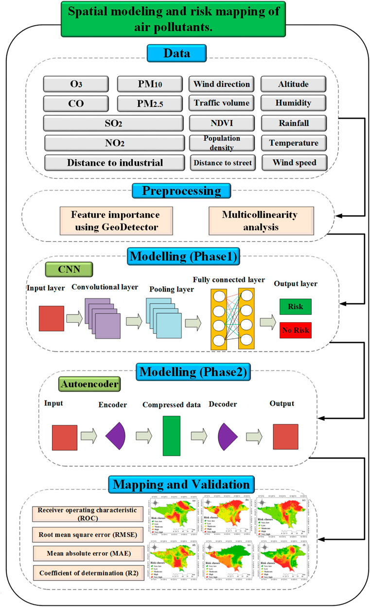
Figure 1. Methodology for spatial modeling and risk mapping of air pollutants.

2.2 Study area

Tehran city (the capital of Iran) is located at 35^° 36′to 35^° 44′north latitude and 51^° 17′to 51^° 33′east longitude and an altitude of 1032–1832 m above sea level. The city of Tehran as the most populous city in Iran (9,039,000) in the last 2 decades due to reasons such as the unsustainable development of industrialization and urbanization, the ever-increasing growth of the transport fleet, and the emission of their pollutants, ineffective national environmental air quality standards, and dust storms. The Middle East has faced severe air pollution, especially (PM₁₀, PM_2.5, O₃, NO₂, SO₂, and CO) (Yousefian et al., 2020). In general, 20% of Iran’s energy is consumed in Tehran. The mountain ranges surrounding the city of Tehran stop the flow of humid wind to the capital, so in winter, the cold weather and lack of wind cause the polluted air to be trapped inside the city (Naddafi et al., 2012). Urban space structures are deeply connected with the urban transportation system (Rodrigue, 2020). The statistics of Tehran indicate the high rate of land consumption in this city, which has caused a high growth in the area and size of the town, which has caused an increase in the distance and the amount of transportation (private cars and public transportation) to carry out administrative and educational activities, and entertainment, in Tehran. Figure 2 displays the geographic location of the study area in Tehran province, Iran, highlighting the air quality control monitoring stations and meteorological stations.

Figure 2

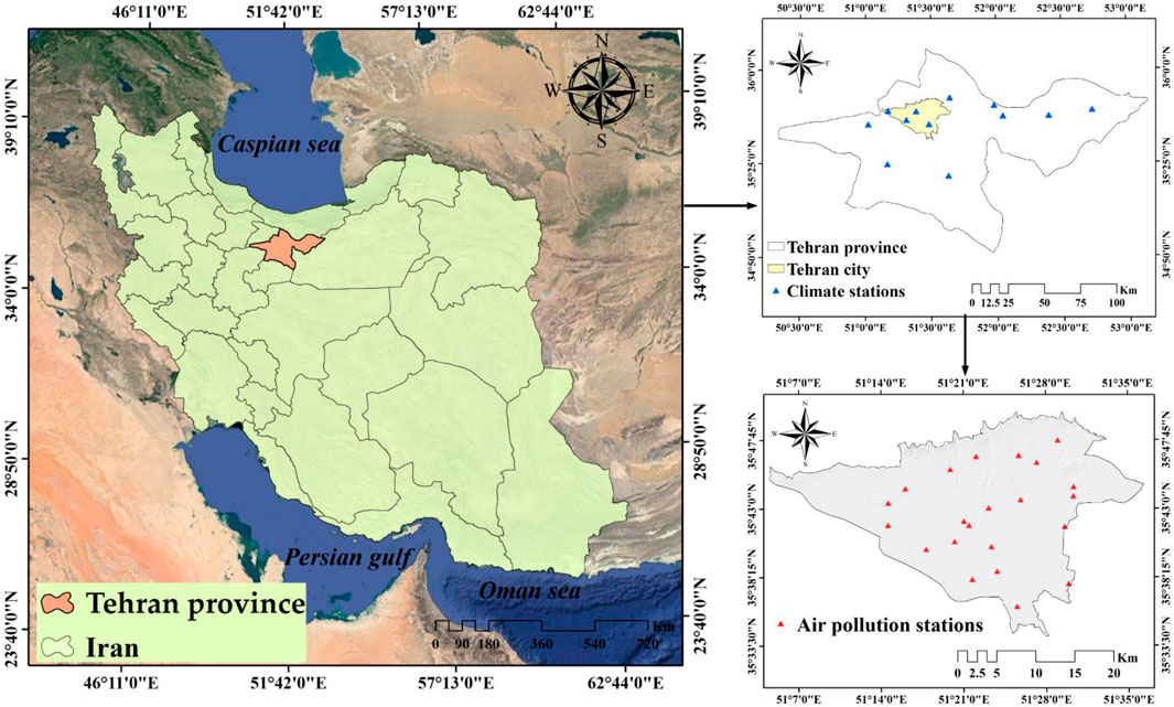
Figure 2. Study area with air pollution and climate stations.

2.3 Air pollutants

Air pollutants can be categorized as either natural or anthropogenic and can be classified as primary or secondary. Primary pollutants are released directly into the atmosphere from a particular source, retaining the same composition. On the other hand, secondary pollutants are not directly released into the atmosphere and are formed in case of a reaction or interaction of primary pollutants or become another compound in the atmosphere, such as photochemical smog (Bhargav, 2020). Six pollutants, PM_2.5, PM₁₀, SO₂, NO₂, O₃, and CO, are considered for this research. Air pollution is a challenging environmental issue that endangers the health and wellbeing of people worldwide, comprising a complex blend of gaseous components and suspended particles (Özbay, 2012; Bergstra et al., 2018). Air quality in cities in developing countries has gradually deteriorated due to rapid urbanization, population growth, and industrialization (Turalıoğlu et al., 2005). The annual average concentration of air pollutants in Tehran was measured from 1 January 2012, to 1 January 2022, using data collected from 23 air quality monitoring stations located in the city. The characteristics of the six pollutants are shown in Table 1, and the trends of the data in the years 2012–2022 are shown in Figure 3. Maps related to the concentration of pollutants were prepared using kriging interpolation in ArcGIS 10.8 software with a pixel size of 30 × 30 m (Figure 4). For modeling, high-risk areas for each pollutant were converted into occurrence points (with a target value of 1) and the low-risk regions into non-occurrence points (with a target value of 0). In the following, each of these parameters will be explained.

➢ Particulate Matter (PM)

Table 1

Table 1. Characteristics of the six air pollutants.

Figure 3

Figure 3. The trend of air pollutant concentrations from 2012 to 2022.

Figure 4

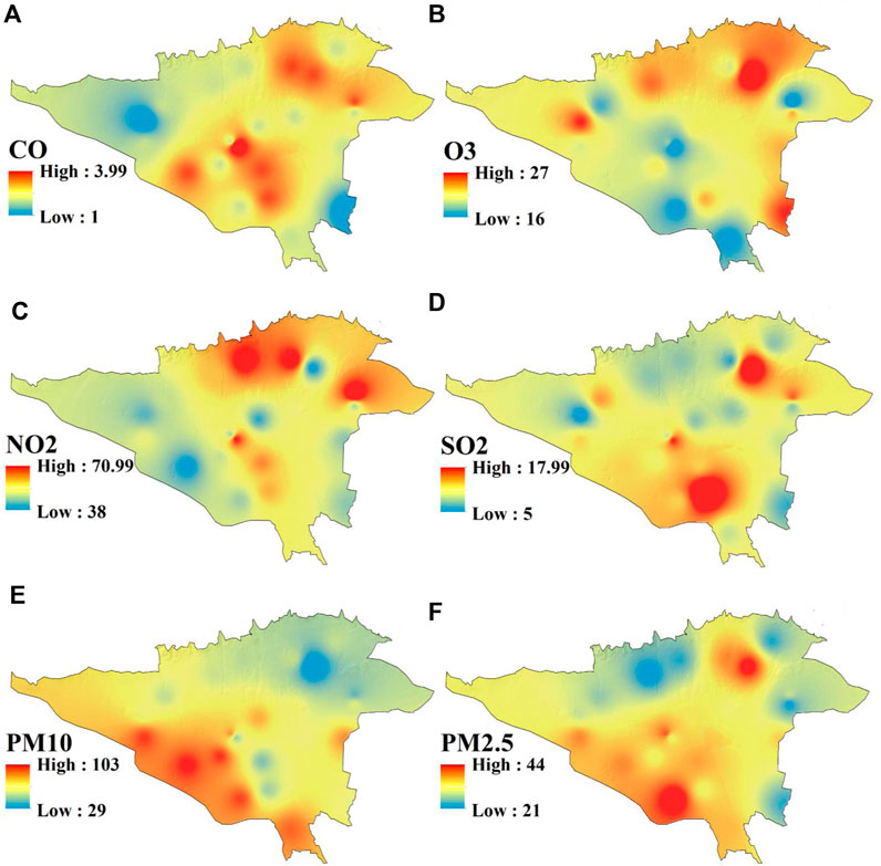
Figure 4. Air pollutant concentration maps: (A) CO, (B) O₃, (C) NO₂, (D) SO₂, (E) PM₁₀, and (F) PM_2.5.

Suspended particles include large particles (PM₁₀) and fine particles (PM_2.5), associated with lung cancer and asthma. PM₁₀ can settle in the bronchi and lungs, and PM_2.5 is the most minor and most dangerous type of suspended particle and can penetrate deep into the respiratory system (Quercia et al., 2015). PM_2.5 particles are mainly caused by fuel combustion, construction dust, and vehicle exhaust, which cause dust-haze. All types of manufactured combustion and some industrial processes are among the most common human sources of PM₁₀ (Özbay, 2012).

➢ Sulfur Dioxide (SO₂)

SO₂ is mainly obtained through the combustion of fossil fuels, biomass burning, and melting ores containing sulfur (Santosa et al., 2008). It is also released through industrial activities and is considered among the harmful gases that affect human, animal, and plant life (Manisalidis et al., 2020). The release of SO₂ in industrial regions can result in serious health concerns such as respiratory irritation, bronchitis, mucus production, bronchospasm, skin redness, eye and mucous membrane damage, and deterioration of cardiovascular health (Chen et al., 2007). Moreover, the environmental consequences of SO₂ include acid rain and soil acidification (Manisalidis et al., 2020).

➢ Nitrogen Oxide (NO₂)

NO₂ is a common traffic-related pollutant that originates from automobile engines, and it is one of the most prevalent air pollutants found in urban regions (Dragomir et al., 2015; Richmond-Bryant et al., 2017). NO₂ is one of the compounds that lead to adverse effects on the environment and human health (Mavroidis and Ilia, 2012), disrupting the sense of smell, burning eyes, throat, and nose, reducing visibility and changing the color of the fabric (Chen et al., 2007).

➢ Carbon Monoxide (CO)

CO is produced due to incomplete or inefficient fuel combustion and affects the blood oxygen transfer in the body and heart (Quercia et al., 2015). CO gas emission and production sources encompass all combustion sources, including motor vehicles, power plants, waste incinerators, domestic gas boilers, and cookers (Vakkilainen, 2017; Manisalidis et al., 2020).

➢ Ozone (O₃)

O₃ is a secondary photochemical pollutant resulting from the oxidation of volatile organic compounds, including benzene, in nitrogen oxides. This colorless, pungent, and reactive gas is the primary component of smog, which is mainly attributed to automobile emissions in urban regions. The concentration of O₃ in urban areas typically increases in the morning, reaches its peak in the afternoon, and decreases at night (Yerramilli et al., 2011).

2.4 Effective factors

The influential factors in this research include meteorological data (rainfall, temperature, humidity, wind direction, and wind speed), altitude, NDVI, distance from street, distance from industrial areas, traffic volume, and population density (Delavar et al., 2019; Shogrkhodaei et al., 2021). Each of the mentioned factors was prepared with a 30 × 30 m pixel size in ArcGIS 10.8 software (Figure 5). In the following, each practical criterion for air pollution has been examined.

• Meteorology data

Figure 5

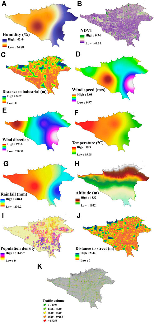
Figure 5. Factors affecting air pollution levels: (A) Humidity, (B) NDVI, (C) Distance to industrial, (D) Wind speed, (E) Wind direction, (F) Temperature, (G) Rainfall, (H) Altitude, (I) Population density, (J) Distance to street, and (K) Traffic volume.

Air pollution has two natural and human causes, natural causes include volcanic eruptions and severe drought, and human activities include motor vehicle emissions, industry, and the burning of agricultural lands and forests, which cause the release of various types of pollutants with multiple characteristics and effects (Sakti et al., 2023). Pollutants in the atmosphere can be dispersed or diluted under various meteorological conditions, such as rainfall, air temperature, and wind speed (Özbay, 2012). Meteorological data, such as wind speed, wind direction, precipitation, temperature, and humidity, were collected from the National Meteorological Organization. The data were obtained from 12 stations and represented the annual average between 2012 and 2022. The kriging interpolation technique was used in ArcGIS 10.8 to create these maps, with a pixel size of 30 * 30 m. The following discusses the impact of meteorological parameters on air pollutants.

➢ Rainfall

Rainfall is one of the main factors of meteorological conditions that affect air quality and has a specific inhibitory effect on air pollutants (Guo and Jiang, 2020; Shukla et al., 2008). Rainfall can affect the concentration of air pollutants by removing gaseous pollution and deposition of suspended particles through atmospheric chemical processes (Kayes et al., 2019).

➢ Temperature

Temperature plays a crucial role in urban air quality, directly influencing gas properties, heterogeneous chemical reaction rates, and the gas-to-particle partitioning process (Aw and Kleeman, 2003). Sunlight and high temperatures stimulate chemical reactions in pollutants and increase smog. The effect of temperature on air pollutants is such that an increase in temperature increases the dispersion and decreases the concentration of contaminants (Shogrkhodaei et al., 2021).

➢ Humidity

Humidity, as one of the meteorological parameters, plays an essential role in air pollutants (their concentration and dispersion) in the urban environment (Endeshaw and Endeshaw, 2020). Most pollutants negatively correlate with relative humidity, so the amount of air pollutants decreases with the increase in humidity (Kayes et al., 2019).

➢ Wind speed and direction

Air quality is affected by wind speed. One case is that wind speed reduces the concentration of pollutants and dilutes them (in areas with higher concentrations). Another issue is that wind speed leads to the entry of contaminants from further distances and increases the concentration of pollutants in an area with a lower concentration (Oleniacz et al., 2016).

• NDVI

Urban vegetation impacts air quality by affecting the sedimentation and dispersion of pollutants (Janhäll, 2015). Urban trees and vegetation are considered an ecosystem regulating service in removing air pollutants (Setälä et al., 2013). The NDVI is a primary indicator of the physiological properties of land vegetation. The NDVI standard was prepared using Landsat-8 satellite images in Google Earth Engine (GEE) (https://earthengine.google.com/) as an annual average from 2012 to 2022. NDVI index was calculated using Eq. 1.

$\text{NDVI}=\frac{\left(\text{NIR}–\text{Red}\right)}{\left(\text{NIR}+\text{Red}\right)}(1)$

In this equation, the symbol NIR denotes the reflectance in the near-infrared band, and the symbol Red represents the reflectance in the red band. By taking the difference and sum of these reflectance values, the NDVI equation normalizes the values and produces an index that ranges from −1 to +1.

•Altitude

Air pollution is affected by the change in altitude, so the increase in altitude causes an increase in sunlight and causes the problem of photochemical smog (U.S. EPA, 1978). This research prepared the height through a digital elevation model (DEM) with a pixel size of 30 × 30 m through the SRTM (Shuttle Radar Topography Mission) image in GEE platform.

• Distance to industrial areas

Industrial sources located inside and close to city borders are among the influential primary factors of urban air pollution (Hosseini and Shahbazi, 2016). Heavy industry causes the release of many dangerous pollutants in the air that affect health (Bergstra et al., 2018). Industrial areas were extracted through land use layers of industrial areas with a scale of 1:10,000. Subsequently, the aforementioned criterion was transformed into a raster map with a pixel resolution of 30 × 30 m by employing the Euclidean distance function in ArcGIS 10.8.

•Distance to street

Motor vehicles produce more air pollutants than any other human activity. Motor vehicle emissions from roads can be considered as a mobile line source with an emission rate per unit of road length (Oji and Adamu, 2020). Therefore, the distance from the measurement location to the roads affects the air quality near the streets (Dragomir et al., 2015). The data relating to the roads of Tehran was extracted through the open street map (OSM) (https://www.openstreetmap.org) with a scale of 1:100,000 in 2022. Subsequently, the mentioned criterion was transformed into a raster map with a pixel resolution of 30 × 30 m by utilizing the Euclidean distance function within the ArcGIS 10.8 software.

• Traffic volume

Urban air pollution is primarily caused by traffic emissions (Guarnieri and Balmes, 2014). Monitoring data about pollution near roads shows hot pollution spots in high-traffic areas (Samet, 2007). Traffic congestion increases vehicle emissions, decreases air quality, and increases air pollutants, including CO, CO₂, nitrogen oxides (NO_x), and PM, which cause complications such as death to drivers, passengers, and people who live near the main roads (Zhang and Batterman, 2013). Data on the traffic volume in Tehran city were obtained from the Tehran Traffic Control Company. The data represent the average traffic volume between 2015 and 2020.

• Population density

The expansion of urban areas and population growth has a significant adverse effect on ambient air quality (Kumar et al., 2016), as the rise in population is linked to an increase in the number of vehicles (traffic density) and industrial and commercial operations (Shogrkhodaei et al., 2021). This factor was obtained based on the data from Iran Statistics Center in 2017.

2.5 Methods

2.5.1 Multicollinearity analysis

The problem of multicollinearity arises due to a correlation (strong relationship) between predictors and their lack of independence in a data set. In the models derived from these data, if multicollinearity is not checked, it may lead to wrong analyzes (Garg and Tai, 2013). Variance Inflation Factor (VIF) is a method used to identify multicollinearity in a regression model (Kim, 2019), and a VIF more significant than 10 indicates the presence of multicollinearity (Chen et al., 2018 Eq. 2).

$\text{VIF}=\frac{1}{\text{Tolerance}}=\frac{1}{1-{\mathrm{R}}^2}(2)$

In the abovementioned equation, the symbol tolerance represents tolerance, and R² is the R-squared value of the regression.

2.5.2 Feature importance using GeoDetector method

GeoDetector is a method used to identify and exploit geographic differences and determines the number of driving forces, influencing factors, and multi-factor interactions (Wang and Xu, 2017). This method does not include complex parameter-setting procedures, nor is it limited to the assumptions of classical linear statistical techniques. In this method, if an independent variable significantly affects another independent variable, it will show spatial distribution (Zhang et al., 2022). GeoDetector has four distinct functions: agent detection, interaction detection, hazard detection, and ecological detection (Wang and Xu, 2017). A factor detector is used to detect the spatial heterogeneity of the dependent variable Y and to evaluate the explanatory ability of the independent variable X on Y. The factor detector assesses the effectiveness of the derived q value in capturing the relationship between the variables. The q values obtained from GeoDetector allow the measurement of spatial variations and factor analysis (Jia et al., 2021). The value of $q_x$ was obtained from Eqs 3–5.

${\mathrm{q}}_{\mathrm{x}}=1-\frac{\text{SSW}}{\text{SST}}(3)$

$SSW={\displaystyle {\sum }_{h=1}^l}{N}_h{{\sigma }_h}^2(4)$

$\text{SST}=\mathrm{N}{\mathrm{\sigma }}^2(5)$

Where SSW denotes the sum of the local variance, while SST represents the global variance. The variable h stands for the number of independent variable categories, $N_h$ and N denote the number of units in zone h and the entire area, respectively. The variable ${{\sigma }_h}^2$ represents the variance of Y in zone h, and ${\mathrm{\sigma }}^2$ denotes the global variance of Y in the entire region.

2.5.3 Convolutional neural network (CNN) algorithm

The traditional ANN in the analysis of complex networks faced the challenge of slowing down the learning process, which Bengio proposed to overcome by a CNN, a neural network that finds local connections between layers (Lu et al., 2017). CNN has achieved remarkable results in various areas of pattern recognition and is particularly useful in reducing the number of parameters in ANN (Albawi et al., 2017). CNN is one of the most widely used deep learning algorithms suitable for spatial data analysis (Khosravi et al., 2020). A CNN architecture generally consists of convolutional, pooling, and fully connected layers (like standard layers in ANN) (Pham et al., 2020). The following is a description of the structure of each layer (Ajit et al., 2020):

➢ The convolutional layer is the most basic and essential in CNN architecture. This layer performs convolution or multiplication operations on the pixel matrix generated for the target image, resulting in an activation map for that image. The activation map stores all the image’s unique features and helps reduce the amount of processed data, which is one of its primary benefits.

➢ Pooling is a crucial layer that helps reduce the activation map’s dimensions while preserving essential features and decreasing spatial invariance. By reducing the number of learnable features, this layer addresses the issue of overfitting. Pooling also enables CNN to combine all dimensions of an image, allowing it to correctly identify the desired object even if its shape is not in the correct position.

➢ The final layer in the neural network is the fully connected layer, which receives input from the previous layers. All the computations and reasoning are performed in this layer of the data.

2.5.4 Autoencoder (AE) algorithm

AE are neural networks that automatically learn useful features and representations from data (Pinaya et al., 2020). AE is also an unsupervised approach to the neural network method. It does not require data labeling with an operational logic that trains input vectors to be reconstructed as output vectors (Sewani and Kashef, 2020). AE can be used for dimensionality reduction, denoising data, generative modeling, and pre-training deep learning neural networks (Pinaya et al., 2020). An encoder and a decoder make AE architecture. An AE layer has an encoder and a decoder according to Eqs 6, 7, respectively (Zavrak and İskefiyeli, 2020).

$\mathrm{h}=\mathrm{\sigma }\left({\mathrm{W}}_{\text{xh}}\mathrm{x}+{\mathrm{b}}_{\text{xh}}\right)(6)$

$\mathrm{z}=\mathrm{\sigma }\left({\mathrm{w}}_{\text{hx}}\mathrm{x}+{\mathrm{b}}_{\text{hx}}\right)(7)$

In the given equations, b and W are referred to as the bias and weight of the neural network, respectively. The symbol σ represents a non-linear transformation function.

2.5.5 Implementing models

The integrated model was implemented using Python in Google Colab, a cloud-based Python development environment. The input data underwent normalization between zero and one to ensure consistent scaling across the different spatial features. This normalization step helps improve the training efficiency and convergence of the model. The experiments and analyses were conducted on a Windows 10 desktop PC with an Intel i7 processor and 16 GB of RAM. The input data was divided into training and testing sets using a 70–30 split. The training set, comprising 70% of the data, was used for model training and parameter optimization. The remaining 30% of the data was reserved for testing the trained model’s performance and evaluating its predictive accuracy. In this research, our objective centered on regression and prediction tasks, for which we employed a 1D CNN model architecture. The implemented CNN model was configured with the following parameters: kernel size set to 3, activation function using ReLU, optimizer utilizing Adam, loss function defined as mean squared error (MSE), an epoch count of 400, batch size set to 16, and verbosity level configured to 2 for detailed logging during training.

2.5.6 Validation methods

To extend the model’s applicability to unfamiliar outputs, it is necessary to assess its performance by comparing the predicted outcomes from each model with the actual results (Mombeini and Yazdani-Chamzini, 2015). In this study, various indicators such as RMSE, MAE, R², and ROC-AUC are employed to evaluate the effectiveness of the model’s construction.

➢ RMSE and MAE

RMSE and MAE are indicators that calculate the error between the actual and predicted values (Farahani et al., 2022). The primary difference between MAE and RMSE indices is that MAE assigns equal weight to all errors. Conversely, RMSE penalizes variance by giving more weight to errors with larger absolute values than errors with smaller values (Chai and Draxler, 2014). RMSE and MAE were calculated according to Eqs 8, 9.

$\text{RMSE}=\sqrt{\frac{{\displaystyle {\sum }_{\mathrm{i}=1}^{\mathrm{n}}}{\left({\mathrm{A}}_{\mathrm{i}}-{\mathrm{P}}_{\mathrm{i}}\right)}^2}{\mathrm{N}}}(8)$

$\text{MAE}=\frac{{\displaystyle {\sum }_{\mathrm{i}=1}^{\mathrm{n}}}\left|\left({\mathrm{A}}_{\mathrm{i}}-P_i\right)\right|}{\mathrm{N}}(9)$

In the above equations, ${\mathrm{A}}_{\mathrm{i}}$ represents the observed value, $P_i$ represents the predicted value, and N is the number of samples.

➢ R²

R² is the variance ratio in the dependent variable that the independent variables can explain (An et al., 2020; Chicco et al., 2021). R² was calculated according to Eq. 10.

${\mathrm{R}}^2=1-\frac{{\sum }_{\mathrm{i}=1}^{\mathrm{n}}{\left({\mathrm{A}}_{\mathrm{i}}-{\mathrm{P}}_{\mathrm{i}}\right)}^2}{{\sum }_{\mathrm{i}=1}^{\mathrm{n}}{\left({\mathrm{A}}_{\mathrm{i}}-\overline{{\mathrm{A}}_{\mathrm{i}}}\right)}^2}(10)$

In this equation, ${\mathrm{A}}_{\mathrm{i}}$ is the observed value, $P_i$ is the predicted value, and $\overline{{\mathrm{A}}_{\mathrm{i}}}$ is the average of the observed set.

➢ ROC curve

The ROC is a prominent method for evaluating spatial models and a standard tool for determining the accuracy of output maps (Shogrkhodaei et al., 2021). The ROC curve plots the false positive rate (FPR) on the x-axis (Eq. 11) against the true positive rate (TPR) on the y-axis (Eq. 12) to measure the area under the curve (AUC) as the true-false thresholds change (Pham et al., 2020).

$\mathrm{x}=1-\frac{\text{TN}}{\text{FP}+\text{TN}}(11)$

$\mathrm{y}=\frac{\text{TP}}{\text{FN}+\text{TP}}(12)$

In this equation, the four data categories in the confusion matrix are TN (True Negative), TP (True Positive), FN (False Negative), and FP (False Positive) (Davis and Goadrich, 2006). AUC is between 0 and 1 (Farahani et al., 2022).

3 Results

3.1 Result of multicollinearity test

A multicollinearity test was performed to assess the presence of multicollinearity among the independent variables utilized in the geographic modeling and risk mapping of the six air contaminants. The results of the test, presented in Table 2, indicate the levels of VIF for each independent variable. From the results, it can be observed that none of the independent variables have VIF values exceeding the threshold limit of 10. This indicates no severe multicollinearity among the independent variables, suggesting that they can be considered individually and collectively in the spatial modeling and risk mapping analysis. The VIF values, ranging from 1.07 to 6.80, indicate that the independent variables have relatively low to moderate levels of correlation with each other. This suggests that the variables provide unique information and do not excessively duplicate each other’s predictive power.

Table 2

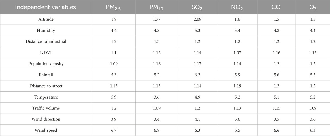
Table 2. Multicollinearity test results on factors affecting air pollution.

3.2 Result of feature importance

The GeoDetector method was employed to determine the importance of different parameters on air pollutants (Figure 6). The analysis revealed distinct findings for each pollutant. CO, temperature, wind speed, and wind direction emerged as the most significant parameters. Variations notably influenced the levels of CO in these factors. In the case of O₃, humidity, precipitation, and altitude were identified as the primary criteria affecting its concentration. Altitude plays a crucial role in the formation and distribution of ozone in the atmosphere.

Figure 6

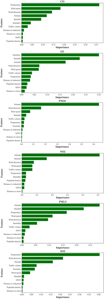
Figure 6. Feature importance results using GeoDetector.

Conversely, for PM₁₀, altitude, wind direction, and wind speed were deemed the most influential parameters. These factors influenced the dispersion and transport of PM₁₀ particles. Regarding NO₂, altitude, rainfall, and wind direction were found to have the most significant impact. Altitude affected the vertical distribution of NO₂, while rainfall and wind direction influenced its dispersion and movement. Similarly, for PM_2.5, altitude, rainfall, and temperature were identified as the key parameters. Altitude affected the vertical distribution of PM_2.5 particles, while rainfall and temperature were crucial in their formation and dispersion. Lastly, for SO₂, temperature, wind direction, and altitude were determined as the most important parameters. Temperature played a role in the chemical reactions involving SO₂, while wind direction and altitude affected its transport and dispersion. In general, altitude, wind direction, wind speed, rainfall, and temperature parameters had the most significant effect on pollutants in the study area.

3.3 Model development

The AE, comprising encoder and decoder layers, is a pre-training step to learn a compact and efficient representation of the input data. The CNN, however, is designed to capture spatial patterns and dependencies within the pollutant data. The input data includes various spatial features such as altitude, humidity, distance to industrial areas, NDVI, population density, rainfall, distance to the street, temperature, traffic volume, wind direction, and wind speed. The Autoencoder’s encoded features serve as input to the CNN, which then extracts spatial features. The model’s weights, biases, learning rates, regularization techniques, and dropout rates are randomly initialized and updated during the training process using the Adam optimizer. A loss function is utilized to measure the difference between the predicted pollutant concentrations and the actual measurements to assess the model’s performance. Common regression loss functions, such as mean squared error (MSE), are commonly used. The results of the loss functions for all pollutants, as shown in Figure 7, indicate the convergence and effectiveness of the integrated CNN-AE model. The loss function values for the training and test data decrease throughout training, demonstrating the model’s ability to learn and capture the underlying patterns in the pollutant data. The decreasing trend of the loss function values suggests the model successfully minimizes the discrepancy between the predicted pollutant concentrations and the actual measurements during training. This indicates that the model is learning to make accurate predictions and is effectively capturing the complex relationships within the data. The decreasing loss function values in the training and test data support the notion that the integrated CNN-AE model successfully learns and generalizes to unseen data, highlighting its ability to capture the spatial patterns and dependencies of the air pollutants.

Figure 7

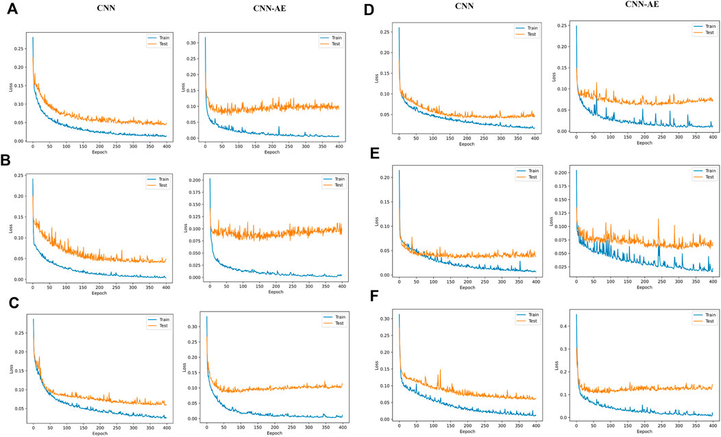
Figure 7. Loss function comparison of CNN and CNN-AE models: (A) CO, (B) O₃, (C) NO₂, (D) SO₂, (E) PM₁₀, and (F) PM_2.5.

Additionally, metrics such as MAE, RMSE, and R² are calculated to assess the accuracy and predictive power of the model (Table 3; Table 4). For the pollutant PM_2.5, the CNN model exhibited reasonably good performance, achieving an R2 of 0.889. The corresponding RMSE and MAE values were 0.166 and 0.046, respectively. However, the CNN-AE model surpassed the CNN model’s performance, demonstrating an improved R² of 0.969. Moreover, the RMSE and MAE values for the CNN-AE model were 0.087 and 0.157, respectively, indicating better accuracy and precision in predicting PM_2.5 concentrations.

Table 3

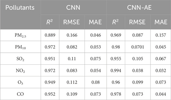
Table 3. Result of air pollution modeling in the training phase.

Table 4

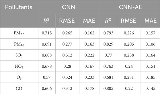
Table 4. Result of air pollution modeling in the test phase.

Regarding the pollutant PM₁₀, both models performed exceptionally well. The CNN model achieved an impressive R² of 0.972, suggesting that the model could explain approximately 97.2% of the PM₁₀ concentration variance. Additionally, the CNN model exhibited low RMSE and MAE values of 0.082 and 0.053, respectively. The CNN-AE model further enhanced the prediction accuracy, yielding an even higher R² of 0.98. The RMSE and MAE values for the CNN-AE model were 0.0701 and 0.045, respectively, indicating a significant improvement over the CNN model. For the pollutant SO₂, both the CNN and CNN-AE models demonstrated commendable performance. The CNN model achieved an R² of 0.951, suggesting that the model could explain approximately 95.1% of the SO₂ concentration variability. The corresponding RMSE and MAE values were 0.11 and 0.075, respectively. The CNN-AE model showed similar performance, with an R2 of 0.955, indicating a comparable ability to explain the variability in SO₂ concentrations. The RMSE and MAE values for the CNN-AE model were 0.105 and 0.067, respectively, demonstrating their effectiveness in predicting SO₂ levels.

Regarding the pollutant NO₂, both models exhibited solid predictive capabilities. The CNN model achieved an R² of 0.972, indicating that the model could explain approximately 97.2% of the NO₂ concentration variability. The RMSE and MAE values were 0.083 and 0.054, respectively, suggesting accurate predictions. The CNN-AE model outperformed the CNN model, attaining an exceptional R² of 0.994. The RMSE and MAE values for the CNN-AE model were significantly lower at 0.038 and 0.032, respectively, indicating superior precision and accuracy in predicting NO₂ concentrations. For the pollutant O₃, both models demonstrated satisfactory performance. The CNN model achieved an R² of 0.949, suggesting that the model could explain approximately 94.9% of the O₃ concentration variability. The RMSE and MAE values were 0.112 and 0.08, respectively. The CNN-AE model improved the prediction accuracy with an R² of 0.96.

Regarding the CO pollutant, the CNN model demonstrated a high level of performance, as indicated by an R² value of 0.952. This suggests that the model’s predictions account for around 95.2% of the variability in CO concentrations. The RMSE and MAE values for CO were calculated as 0.109 and 0.073, respectively. Notably, the CNN-AE further enhanced the accuracy of CO predictions. The CNN-AE model achieved an improved R² value of 0.978, indicating that the model captured approximately 97.8% of the CO concentration variability. The corresponding RMSE and MAE values were calculated as 0.073 and 0.044, respectively.

Moving on to the test data, the CNN exhibited moderate performance with R² values ranging from 0.57 to 0.715 for six pollutants. The RMSE values ranged from 0.265 to 0.324, indicating some difference between the predicted and actual values. The MAE values ranged from 0.162 to 0.233, representing the average absolute difference between predicted and actual values. In contrast, the CNN-AE improved performance on the test data compared to the CNN. It achieved higher R² values ranging from 0.681 to 0.829, indicating a better fit. The lower RMSE values, ranging from 0.205 to 0.281, suggested more accurate predictions. The MAE values ranged from 0.106 to 0.185, indicating a more negligible average absolute difference between predicted and actual values compared to the CNN.

In summary, integrating the AE with the CNN algorithm showed promising results in air quality management. The CNN and CNN-AE models exhibited strong performance in the training phase, with the CNN-AE model consistently outperforming the CNN. Although there was a slight decrease in performance during the testing phase, the CNN-AE model maintained its superiority over CNN. Figure 8 shows the fitting diagram of the training and test data on the target data.

Figure 8

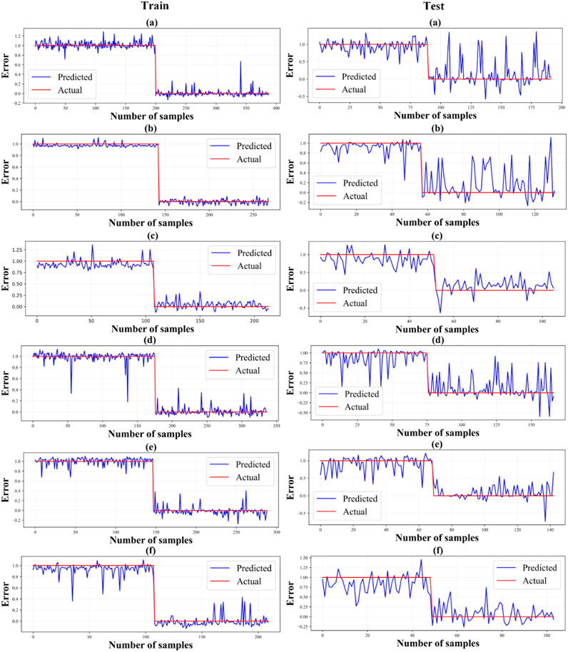
Figure 8. Error diagram in training and test data. (A) CO, (B) O₃, (C) NO₂, (D) SO₂, (E) PM₁₀, and (F) PM_2.5.

3.4 Creation of risk map and validation

Using the trained model, the CNN-AE model estimated pollutant concentrations for each location in the study area. These estimated concentrations were then assigned risk levels to different regions based on classification criteria. The risk levels could be categorized as very low, low, moderate, high, and very high, representing varying degrees of pollution severity (Figure 9). The risk maps were generated by overlaying the estimated pollutant concentrations onto a geographical map of the study area. Each region was color-coded according to the assigned risk level, providing an intuitive visualization of the pollution hotspots and areas of concern, and according to the risk maps generated from the CNN-AE model, the southwest and northeast regions exhibited higher risk levels for CO pollution. Concerning O₃ pollution, elevated risk levels were observed in the north, east, and west areas. The risk of NO₂ pollution was particularly pronounced in the north and central regions. In the case of SO₂ pollution, the risk was concentrated in the south and northeast areas. PM₁₀ pollution posed a higher risk in the west and southwest regions, while PM_2.5 pollution was more prominent in the southern part.

Figure 9

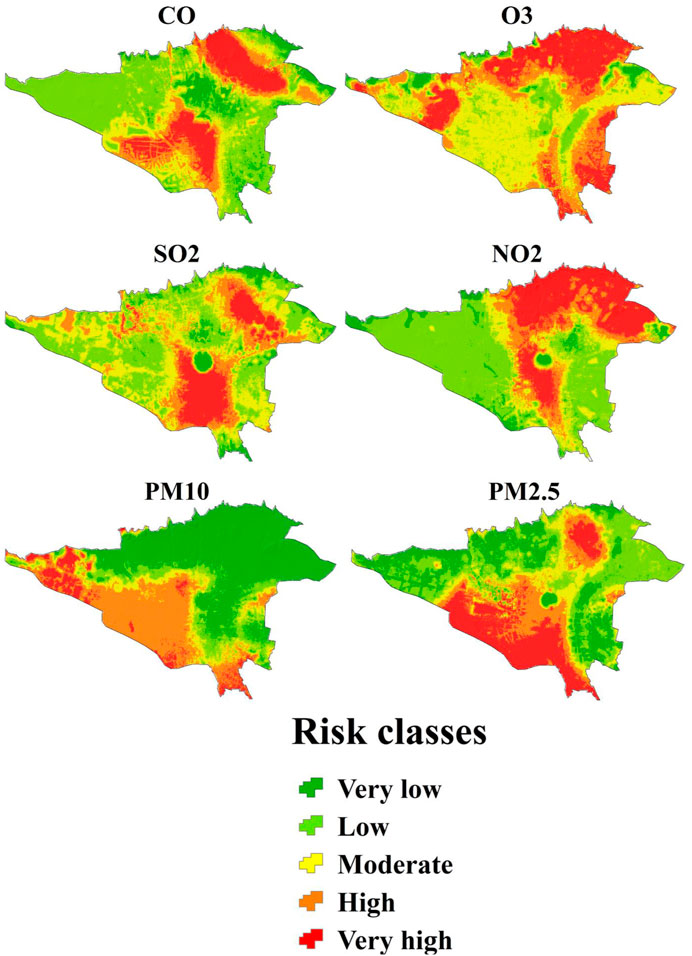
Figure 9. Risk map of different pollutants.

Several evaluation metrics were employed to assess the effectiveness of the risk maps generated by the CNN-AE method, including the ROC curve, AUC, and Youden index J. These metrics were used to analyze the performance of the risk maps in terms of their ability to accurately discriminate between different risk levels. The evaluation results, as presented in Table 5 and Figure 10. For NO₂, an AUC of 0.964 was obtained, indicating a high level of discrimination between different risk levels. The Youden index J was 0.8936, further confirming the model’s ability to identify the optimal threshold for risk classification. The Standard Error was 0.0235, and the 95% Confidence Interval ranged from 0.903 to 0.991, indicating high precision in the risk map. The z statistic value was 19.72, and the significance level was p < 0.0001, demonstrating the statistical significance of the results.

Table 5

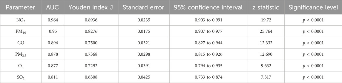
Table 5. Validation result of air pollutants risk mapping.

Figure 10

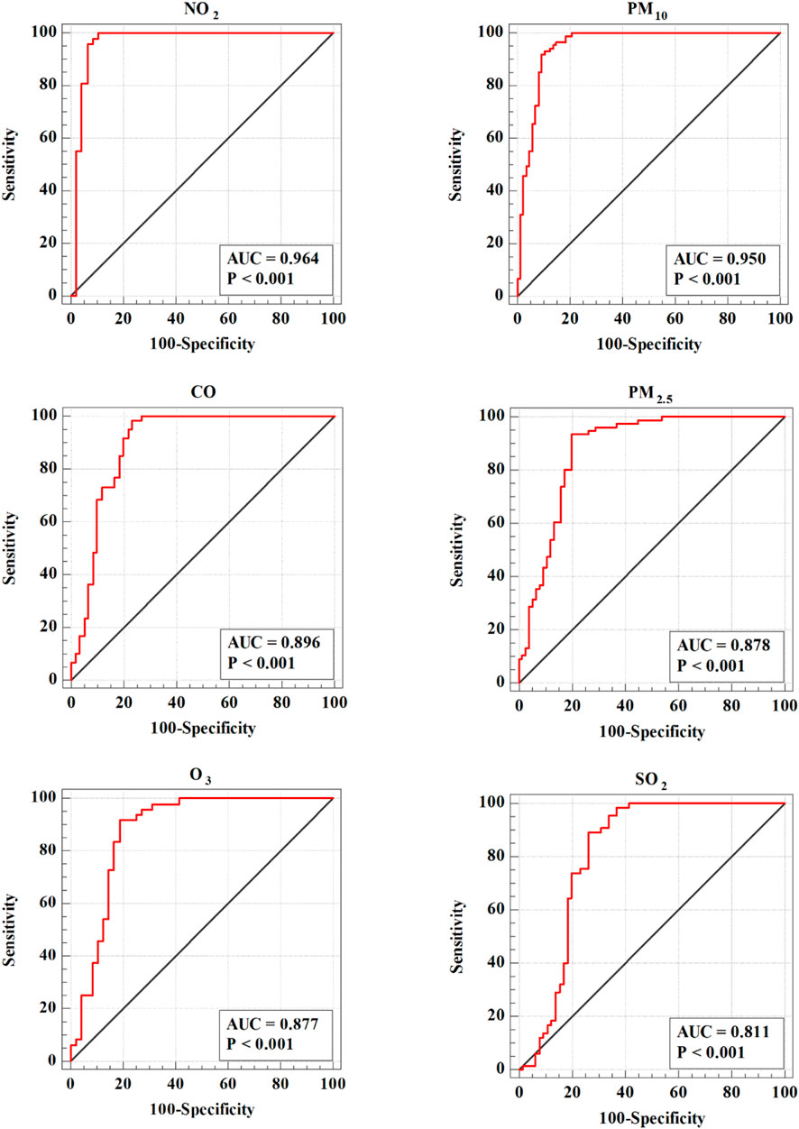
Figure 10. Validation of risk maps by ROC curve.

Similarly, for PM₁₀, an AUC of 0.95 was achieved, indicating good discriminatory power. The Youden index J was 0.8276, highlighting the model’s effectiveness in identifying risk thresholds. The Standard Error was 0.0175, and the 95% Confidence Interval ranged from 0.907 to 0.977, indicating a high confidence level in the risk map. The z-statistic value was 25.764, and the significance level was p < 0.0001, further confirming the statistical significance of the findings. The performance of the CNN-AE algorithm was also evaluated for CO, PM_2.5, O₃, and SO₂. The AUC values for CO, PM_2.5, and O₃ were 0.896, 0.878, and 0.877, respectively, demonstrating moderate to high discriminatory power. The Youden index values were 0.75, 0.7368, and 0.7292, indicating the model’s ability to identify suitable risk thresholds. The Standard Errors were 0.0321, 0.0298, and 0.0391, respectively, showing the precision of the risk maps. The 95% Confidence Intervals ranged from 0.827 to 0.944 for CO, 0.815 to 0.926 for PM_2.5, and 0.794 to 0.935 for O₃, further strengthening the reliability of the risk estimates. The z-statistic values were 12.332, 12.69, and 9.632, respectively, and the significance levels were p < 0.0001 for all three pollutants, underscoring the statistical significance of the observed results. Lastly, for SO₂, an AUC of 0.811 was obtained, indicating an acceptable level of discrimination between risk levels. The Youden index J was 0.6308, suggesting the model’s capability to identify appropriate risk thresholds. The Standard Error was 0.0425, and the 95% Confidence Interval ranged from 0.733 to 0.874, providing a reliable estimate of the risk map. The z statistic value was 7.317, and the significance level was p < 0.0001, affirming the statistical significance of the results. Integrating the AE with the CNN algorithm proved effective in spatial modeling and risk mapping of the six air pollutants. The high AUC values, significant Youden index values, narrow confidence intervals, and low p-values indicate the model’s ability to discriminate between different levels of pollutant risk and its statistical reliability. These results contribute to our understanding of the spatial distribution and potential.

4 Discussion

The study’s outcomes indicate that combining AE with CNN algorithms is a successful approach for spatial modeling and risk mapping of six air pollutants. By combining the strengths of these two techniques, we overcame-overcame the limitations of traditional modeling approaches and achieved more accurate predictions of air pollutant concentrations. This section discusses the key findings, implications, limitations, and potential future directions of the research. One of the major findings of this study is the significant improvement in modeling accuracy achieved through the CNN-AE fusion approach. Integrating the autoencoder allowed for extracting essential features and patterns from the air pollutant data, effectively reducing dimensionality while preserving relevant information (Dairi et al., 2021).

On the other hand, the CNN leveraged the spatial relationships and patterns in the data, enabling more precise modeling of the pollutant concentrations across the study area (Jiang et al., 2022). As a result, the combined model outperformed traditional modeling approaches, as evidenced by the reduced MAE and RMSE values. The superior performance of the CNN-AE model can be attributed to the benefits provided by the AE component. The AE enables the model to learn a compact and meaningful representation of the input data, which enhances its ability to extract relevant features and patterns. This feature extraction capability is significant in air quality management, as various complex and interrelated factors influence pollutant levels (Cheng et al., 2018; Shankar and Parsana, 2022).

The GeoDetector method assessed the importance of different parameters on various air pollutants, revealing crucial insights for policymakers and researchers. For the CO pollutant, the observed influence of temperature, wind speed, and wind direction can be attributed to their impact on the combustion processes and emissions. Higher temperatures may enhance CO’s chemical reactions, increasing pollutant levels (Noyes et al., 2009). Wind speed and direction play a crucial role in the dispersion of CO emissions, affecting the spatial distribution and concentration of the pollutant (Gorai et al., 2015). Regarding the O₃ pollutant, humidity, rainfall, and altitude are important factors. The formation of ozone is primarily influenced by photochemical reactions that occur when nitrogen oxides (NOx) and volatile organic compounds (VOCs) are present in sunlight (Swamy et al., 2012). Humidity and precipitation can influence these reactions by altering the availability of reactants and the rate of chemical transformations (Bell, 2020). Altitude plays a role in determining the amount of solar radiation and the temperature conditions conducive to ozone formation (Zhao et al., 2019). For PM₁₀, altitude, wind direction, and wind speed have significant impacts. Altitude affects the dispersion and transport of PM₁₀ particles, with higher altitudes often leading to increased atmospheric mixing and dilution of pollutants (Li et al., 2019). Wind direction and speed determine the pathways and distances PM₁₀ particles can travel, influencing their spatial distribution and concentration (Wang et al., 2010).

Regarding the NO₂ pollutant, the altitude parameter indicates the vertical distribution of NO₂ emissions (Salmond et al., 2013). Higher emissions released from industrial sources or vehicle exhausts closer to the ground can contribute to increased levels of NO₂ (Richter et al., 2005). Rainfall can play a role in removing NO₂ from the atmosphere through wet deposition, while wind direction influences the spatial distribution and transport of NO₂ emissions (Matejko et al., 2009). For PM_2.5, altitude, rainfall, and temperature exhibit notable effects. Altitude influences the vertical distribution of PM_2.5 particles, with emissions and sources at different heights impacting their ground-level concentration (Peng et al., 2015). Rainfall can remove PM_2.5 particles from the atmosphere, lowering pollutant levels (Nowak et al., 2013). Temperature can influence the chemical reactions and physical processes involved in forming, transforming, and dispersing PM_2.5 particles (Su et al., 2020). Finally, for the SO₂ pollutant, temperature affects the rates of chemical reactions involving SO₂. Higher temperatures can facilitate the conversion of SO₂ into other secondary pollutants, such as sulfuric acid aerosols (He et al., 2014). Wind direction and height play a role in the transport and dispersion of SO₂ emissions, influencing the spatial distribution and concentration of the pollutant (Hong et al., 2021).

Our analysis revealed higher risk levels of SO₂ pollution in Tehran’s northeastern, central, and southern regions. This heightened risk can be attributed to the concentration of industrial zones and higher population density in these areas. Industrial activities and dense urban settlements are known to be significant sources of SO₂ emissions, contributing to elevated pollution levels. Our findings depicted higher risk levels of PM_2.5 and PM₁₀ pollution in Tehran’s southwestern and southern regions. This pattern can be attributed to the concentration of industrial areas in these zones. Industrial activities are a significant source of particulate matter emissions, contributing to higher pollution levels in nearby residential and commercial areas. The risk maps for CO indicated increased risk levels in the southwestern and northeastern parts of Tehran. This observation can be linked to the density of road networks and higher traffic volume in these areas. The combustion of fossil fuels in vehicles releases CO emissions, resulting in elevated concentrations near significant roadways and urban centers. The risk maps for O₃ pollution indicated elevated risk levels in the northern, southern, and eastern parts of Tehran. This heightened risk is associated with increased traffic emissions, NO_x, indirectly contributing to O₃ formation through photochemical reactions. Additionally, Tehran’s central, northeastern, and eastern areas exhibited higher NO₂ concentrations due to population density and increased vehicular traffic.

Despite the valuable insights gained from this research on air quality management using spatial modeling, risk mapping, and the integration of the AE with the CNN algorithm, it is important to acknowledge certain limitations and offer suggestions for future research. Firstly, the accuracy of the models heavily relies on the quality and representativeness of the input data. Any inaccuracies or biases in the monitoring data could affect the reliability of the models and risk maps. Additionally, the spatial criteria used in the analysis are based on existing knowledge and assumptions about factors influencing air pollution. There may be other unaccounted spatial parameters that could affect the models’ accuracy. Future studies could explore incorporating more comprehensive datasets and advanced feature selection techniques to enhance the modeling accuracy.

Furthermore, the evaluation metrics used in this study, such as MAE and RMSE, provide an overall assessment of the modeling performance. However, it is essential to consider additional evaluation measures, such as spatial validation techniques, to assess the goodness of fit and the model’s ability to capture spatial patterns accurately. This can provide further insights into the reliability and generalizability of the risk maps generated. In terms of future directions, this research opens avenues for exploring additional techniques and methodologies to enhance air quality modeling and risk mapping. For example, incorporating spatiotemporal modeling approaches could capture the dynamic nature of air pollution and improve the accuracy of predictions. Furthermore, integrating other machine learning algorithms or hybrid models could yield even better results by leveraging the strengths of different techniques.

The improved spatial modeling and risk mapping techniques developed in this study provide valuable tools for policymakers and environmental regulators to design targeted interventions and implement evidence-based policies for air quality management. By identifying pollution hotspots and understanding the underlying factors contributing to elevated pollutant levels, policymakers can prioritize resources and implement mitigation measures to reduce exposure and protect public health. Furthermore, integrating advanced modeling techniques can enhance the effectiveness of regulatory initiatives to reduce emissions from industrial facilities, transportation networks, and other pollution sources.

The successful fusion of AE with CNN opens up new avenues for air quality modeling and risk assessment research. Future studies could explore further enhancements to the modeling framework by incorporating additional data sources, refining feature extraction algorithms, and integrating spatiotemporal modeling approaches to capture the dynamic nature of air pollution. Additionally, research efforts could focus on investigating the interactions between different pollutants and identifying synergistic effects on human health, ecosystems, and climate change. Furthermore, interdisciplinary collaborations between researchers from various domains, including environmental science, computer science, and public health, can facilitate the development of innovative solutions to address complex air quality challenges.

5 Conclusion

This research presents a novel and innovative approach for spatial modeling and risk mapping of six air pollutants by combining AE with a CNN algorithm. Integrating these two techniques has significantly improved modeling accuracy and the generation of informative risk maps. The research results indicate that the integrated CNN-AE model outperforms the standalone CNN model regarding predictive accuracy. The evaluation of the models on train and test data further confirmed the superiority of the CNN-AE model, as it achieved higher R² values, lower RMSE values, and smaller MAE values than the CNN model. These findings suggest that integrating the AE with the CNN algorithm enhances the model’s ability to capture and utilize the spatial relationships in the pollutant data. In the study area, the pollutants were most influenced by specific parameters, namely, altitude, wind direction, wind speed, rainfall, and temperature, as determined by applying the GeoDetector method.

The risk maps generated by the CNN-AE model indicated distinct pollution patterns across different regions. The southwest and northeast regions showed higher risk levels for CO pollution. Elevated risk levels for O₃ pollution were observed in the north, east, and west areas. The north and central regions exhibited a pronounced risk of NO₂ pollution. The risk of SO₂ pollution was concentrated in the south and northeast areas. PM₁₀ pollution posed a higher risk in the west and southwest regions, while PM_2.5 pollution was more prominent in the southern part. The risk maps generated through the integrated methodology provide valuable insights for air quality management. By visualizing the spatial distribution of the pollutant concentrations, these risk maps help identify high-risk areas and pollution hotspots. This information is crucial for policymakers, environmental agencies, and stakeholders to prioritize mitigation efforts and allocate resources effectively. The risk maps can also support decision-making processes, facilitating the development of targeted interventions to reduce pollutant levels and protect public health. For future research, it is suggested that the CNN-AE model be adapted and validated across diverse geographical regions to ensure generalizability and robustness. Incorporating real-time data from sensors and satellite imagery could enhance the model’s real-time air quality monitoring applicability. Additionally, expanding the methodology to include a broader range of pollutants and investigating the impact of climate change on pollution patterns will provide comprehensive assessments. Linking the risk maps with health impact assessments could offer valuable insights into public health implications, supporting informed policy development.

Data availability statement

The raw data supporting the conclusion of this article will be made available by the authors, without undue reservation.

Author contributions

AB: Conceptualization, Data curation, Formal Analysis, Investigation, Resources, Software, Visualization, Writing–original draft. MM: Conceptualization, Methodology, Project administration, Resources, Supervision, Writing–review and editing. MK: Funding acquisition, Methodology, Resources, Validation, Writing–review and editing.

Funding

The author(s) declare that no financial support was received for the research, authorship, and/or publication of this article.

Conflict of interest

The authors declare that the research was conducted in the absence of any commercial or financial relationships that could be construed as a potential conflict of interest.

Publisher’s note

All claims expressed in this article are solely those of the authors and do not necessarily represent those of their affiliated organizations, or those of the publisher, the editors and the reviewers. Any product that may be evaluated in this article, or claim that may be made by its manufacturer, is not guaranteed or endorsed by the publisher.

References

Abu El-Magd, S., Soliman, G., Morsy, M., and Kharbish, S. (2022). Environmental hazard assessment and monitoring for air pollution using machine learning and remote sensing. Int. J. Environ. Sci. Technol., 1–14. doi:10.1007/s13762-022-04367-6

CrossRef Full Text | Google Scholar

Agarwal, S. K. (2021). Cardiovascular dangers of air pollution. J. Clin. Cardiol. Interv. 2.

Google Scholar

Ajit, A., Acharya, K., and Samanta, A. (2020). “A review of convolutional neural networks,” in 2020 International Conference on Emerging Trends in Information Technology and Engineering (ic-ETITE), Germany, 2020, February, 1–5.

CrossRef Full Text | Google Scholar

Albawi, S., Mohammed, T. A., and Al-Zawi, S. (2017). “Understanding of a convolutional neural network,” in 2017 International Conference on Engineering and Technology (ICET), USA, 2017, August, 1–6.

CrossRef Full Text | Google Scholar

An, G., Xing, M., He, B., Liao, C., Huang, X., Shang, J., et al. (2020). Using machine learning for estimating rice chlorophyll content from in situ hyperspectral data. Remote Sens. 12 (18), 3104. doi:10.3390/rs12183104

CrossRef Full Text | Google Scholar

Aw, J., and Kleeman, M. J. (2003). Evaluating the first-order effect of intraannual temperature variability on urban air pollution. J. Geophys. Res. Atmos. 108 (D12). doi:10.1029/2002jd002688

CrossRef Full Text | Google Scholar

Bank, D., Koenigstein, N., and Giryes, R. (2020). Autoencoders. arXiv preprint arXiv:2003.05991.

Google Scholar

Bekkar, A., Hssina, B., Douzi, S., and Douzi, K. (2021). Air-pollution prediction in smart city, deep learning approach. J. Big Data 8 (1), 161–221. doi:10.1186/s40537-021-00548-1

PubMed Abstract | CrossRef Full Text | Google Scholar

Bell, L. N. (2020). Moisture effects on food's chemical stability. Water Activity Foods Fundam. Appl., 227–253. doi:10.1002/9781118765982.ch9

CrossRef Full Text | Google Scholar

Bell, M. L. (2006). The use of ambient air quality modeling to estimate individual and population exposure for human health research: a case study of ozone in the Northern Georgia Region of the United States. Environ. Int. 32 (5), 586–593. doi:10.1016/j.envint.2006.01.005

PubMed Abstract | CrossRef Full Text | Google Scholar

Bergstra, A. D., Brunekreef, B., and Burdorf, A. (2018). The effect of industry-related air pollution on lung function and respiratory symptoms in school children. Environ. Health 17 (1), 30–39. doi:10.1186/s12940-018-0373-2

PubMed Abstract | CrossRef Full Text | Google Scholar

Bhargav, A. (2020). Air pollution-sources and classification. Op Acc J Bio Sci Res 1 (4). doi:10.46718/jbgsr.2020.01.000022

CrossRef Full Text | Google Scholar

Briggs, D. J., Collins, S., Elliott, P., Fischer, P., Kingham, S., Lebret, E., et al. (1997). Mapping urban air pollution using GIS: a regression-based approach. Int. J. Geogr. Inf. Sci. 11 (7), 699–718. doi:10.1080/136588197242158

CrossRef Full Text | Google Scholar

Bui, T. C., Le, V. D., and Cha, S. K. (2018). A deep learning approach for forecasting air pollution in South Korea using LSTM. doi:10.48550/arXiv.1804.07891

CrossRef Full Text | Google Scholar

Castelli, M., Clemente, F. M., Popovič, A., Silva, S., and Vanneschi, L. (2020). A machine learning approach to predict air quality in California. Complexity 2020, 1–23. doi:10.1155/2020/8049504

CrossRef Full Text | Google Scholar

Chai, T., and Draxler, R. R. (2014). Root mean square error (RMSE) or mean absolute error (MAE)? – Arguments against avoiding RMSE in the literature. Geosci. Model Dev. 7 (3), 1247–1250. doi:10.5194/gmd-7-1247-2014

CrossRef Full Text | Google Scholar

Chen, T. M., Kuschner, W. G., Gokhale, J., and Shofer, S. (2007). Outdoor air pollution: nitrogen dioxide, sulfur dioxide, and carbon monoxide health effects. Am. J. Med. Sci. 333 (4), 249–256. doi:10.1097/maj.0b013e31803b900f

PubMed Abstract | CrossRef Full Text | Google Scholar

Chen, W., Li, H., Hou, E., Wang, S., Wang, G., Panahi, M., et al. (2018). GIS-based groundwater potential analysis using novel ensemble weights-of-evidence with logistic regression and functional tree models. Sci. Total Environ. 634, 853–867. doi:10.1016/j.scitotenv.2018.04.055

PubMed Abstract | CrossRef Full Text | Google Scholar

Cheng, Z., Sun, H., Takeuchi, M., and Katto, J. (2018). “Deep convolutional autoencoder-based lossy image compression,” in 2018 picture coding symposium (PCS) (Germany: IEEE), 253–257.

CrossRef Full Text | Google Scholar

Chicco, D., Warrens, M. J., and Jurman, G. (2021). The coefficient of determination R-squared is more informative than SMAPE, MAE, MAPE, MSE and RMSE in regression analysis evaluation. PeerJ Comput. Sci. 7, e623. doi:10.7717/peerj-cs.623

PubMed Abstract | CrossRef Full Text | Google Scholar

Dairi, A., Harrou, F., Khadraoui, S., and Sun, Y. (2021). Integrated multiple directed attention-based deep learning for improved air pollution forecasting. IEEE Trans. Instrum. Meas. 70, 1–15. doi:10.1109/tim.2021.3091511

PubMed Abstract | CrossRef Full Text | Google Scholar

Davis, J., and Goadrich, M. (2006). “The relationship between Precision-Recall and ROC curves,” in Proceedings of the 23rd International Conference on Machine Learning, China, 2006, June, 233–240.

CrossRef Full Text | Google Scholar

Delavar, M. R., Gholami, A., Shiran, G. R., Rashidi, Y., Nakhaeizadeh, G. R., Fedra, K., et al. (2019). A novel method for improving air pollution prediction based on machine learning approaches: a case study applied to the capital city of Tehran. ISPRS Int. J. Geo-Information 8 (2), 99. doi:10.3390/ijgi8020099

CrossRef Full Text | Google Scholar

Dons, E., Van Poppel, M., Panis, L. I., De Prins, S., Berghmans, P., Koppen, G., et al. (2014). Land use regression models as a tool for short, medium and long term exposure to traffic related air pollution. Sci. Total Environ. 476, 378–386. doi:10.1016/j.scitotenv.2014.01.025

PubMed Abstract | CrossRef Full Text | Google Scholar

Dragomir, C. M., Voiculescu, M., Constantin, D. E., and Georgescu, L. P. (2015). Prediction of the NO2 concentration data in an urban area using multiple regression and neuronal networks AIP Conference Proceedings. AIP Publ. LLC 1694 (1), 040003. doi:10.1063/1.4937255

CrossRef Full Text | Google Scholar

Endeshaw, M. F. L., and Endeshaw, L. (2020). Influence of temperature and relative humidity on air pollution in addis ababa, Ethiopia. J. Environ. Earth Sci. 2 (02), 19–25. doi:10.30564/jees.v2i2.2286

CrossRef Full Text | Google Scholar

Farahani, M., Razavi-Termeh, S. V., and Sadeghi-Niaraki, A. (2022). A spatially based machine learning algorithm for potential mapping of the hearing senses in an urban environment. Sustain. Cities Soc. 80, 103675. doi:10.1016/j.scs.2022.103675

CrossRef Full Text | Google Scholar

Faridi, S., Niazi, S., Yousefian, F., Azimi, F., Pasalari, H., Momeniha, F., et al. (2019). Spatial homogeneity and heterogeneity of ambient air pollutants in Tehran. Sci. Total Environ. 697, 134123. doi:10.1016/j.scitotenv.2019.134123

PubMed Abstract | CrossRef Full Text | Google Scholar

Garg, A., and Tai, K. (2013). Comparison of statistical and machine learning methods in modelling of data with multicollinearity. Int. J. Model. Identif. Control 18 (4), 295–312. doi:10.1504/ijmic.2013.053535

CrossRef Full Text | Google Scholar

Ge, Y., Fu, Q., Yi, M., Chao, Y., Lei, X., Xu, X., et al. (2022). High spatial resolution land-use regression model for urban ultrafine particle exposure assessment in Shanghai, China. Sci. Total Environ. 816, 151633. doi:10.1016/j.scitotenv.2021.151633

PubMed Abstract | CrossRef Full Text | Google Scholar

Ghorbanzadeh, O., Meena, S. R., Blaschke, T., and Aryal, J. (2019). UAV-based slope failure detection using deep-learning convolutional neural networks. Remote Sens. 11 (17), 2046. doi:10.3390/rs11172046

CrossRef Full Text | Google Scholar

Gorai, A. K., Tuluri, F., Tchounwou, P. B., and Ambinakudige, S. (2015). Influence of local meteorology and NO2 conditions on ground-level ozone concentrations in the eastern part of Texas, USA. Air Qual. Atmos. Health 8, 81–96. doi:10.1007/s11869-014-0276-5

PubMed Abstract | CrossRef Full Text | Google Scholar

Guarnieri, M., and Balmes, J. R. (2014). Outdoor air pollution and asthma. Lancet 383 (9928), 1581–1592. doi:10.1016/s0140-6736(14)60617-6

PubMed Abstract | CrossRef Full Text | Google Scholar

Gulliver, J., and Briggs, D. (2011). STEMS-Air: a simple GIS-based air pollution dispersion model for city-wide exposure assessment. Sci. Total Environ. 409 (12), 2419–2429. doi:10.1016/j.scitotenv.2011.03.004

PubMed Abstract | CrossRef Full Text | Google Scholar

Guo, R., and Jiang, Y. (2020). Effects of precipitation on air pollution in spring and summer in lanzhou. E3S Web Conf. 194, 04007. doi:10.1051/e3sconf/202019404007

CrossRef Full Text | Google Scholar

He, H., Wang, Y., Ma, Q., Ma, J., Chu, B., Ji, D., et al. (2014). Mineral dust and NOx promote the conversion of SO2 to sulfate in heavy pollution days. Sci. Rep. 4 (1), 4172. doi:10.1038/srep04172

PubMed Abstract | CrossRef Full Text | Google Scholar

Hogland, J., and Anderson, N. (2017). Function modeling improves the efficiency of spatial modeling using big data from remote sensing. Big Data Cognitive Comput. 1, 3. doi:10.3390/bdcc1010003

CrossRef Full Text | Google Scholar

Hong, Q., Liu, C., Hu, Q., Xing, C., Tan, W., Liu, T., et al. (2021). Vertical distributions of tropospheric SO2 based on MAX-DOAS observations: investigating the impacts of regional transport at different heights in the boundary layer. J. Environ. Sci. 103, 119–134. doi:10.1016/j.jes.2020.09.036

CrossRef Full Text | Google Scholar

Hosseini, V., and Shahbazi, H. (2016). Urban air pollution in Iran. Iran. Stud. 49 (6), 1029–1046. doi:10.1080/00210862.2016.1241587

CrossRef Full Text | Google Scholar

Hu, K., Sivaraman, V., Bhrugubanda, H., Kang, S., and Rahman, A. (2016). “SVR based dense air pollution estimation model using static and wireless sensor network,” in 2016 ieee sensors (China: IEEE), 1–3.

CrossRef Full Text | Google Scholar

Hu, X., Chu, L., Pei, J., Bian, J., and Liu, W. (2021). Deep learning model complexity: concepts and approaches.

Google Scholar

Janhäll, S. (2015). Review on urban vegetation and particle air pollution – deposition and dispersion. Atmos. Environ. 105, 130–137. doi:10.1016/j.atmosenv.2015.01.052

CrossRef Full Text | Google Scholar

Jia, W. J., Wang, M. F., Zhou, C. H., and Yang, Q. H. (2021). Analysis of the spatial association of geographical detector-based landslides and environmental factors in the southeastern Tibetan Plateau, China. PLOS ONE 16 (5), e0251776. doi:10.1371/journal.pone.0251776

PubMed Abstract | CrossRef Full Text | Google Scholar

Jiang, Z., Zheng, T., Bergin, M., and Carlson, D. (2022). Improving spatial variation of ground-level PM2.5 prediction with contrastive learning from satellite imagery. Sci. Remote Sens. 5, 100052. doi:10.1016/j.srs.2022.100052

CrossRef Full Text | Google Scholar

Kalajdjieski, J., Zdravevski, E., Corizzo, R., Lameski, P., Kalajdziski, S., Pires, I. M., et al. (2020) Air pollution prediction with multi-modal data and deep neural networks. Remote Sens. 12, 4142, doi:10.3390/rs12244142

CrossRef Full Text | Google Scholar

Kayes, I., Shahriar, S. A., Hasan, K., Akhter, M., Kabir, M. M., and Salam, M. A. (2019). The relationships between meteorological parameters and air pollutants in an urban environment. Glob. J. Environ. Sci. Manag. 5 (3), 265–278.doi:10.22034/GJESM.2019.03.01

CrossRef Full Text | Google Scholar

Khosravi, K., Panahi, M., Golkarian, A., Keesstra, S. D., Saco, P. M., Bui, D. T., et al. (2020). Convolutional neural network approach for spatial prediction of flood hazard at national scale of Iran. J. Hydrology 591, 125552. doi:10.1016/j.jhydrol.2020.125552

CrossRef Full Text | Google Scholar

Kim, J. H. (2019). Multicollinearity and misleading statistical results. Korean J. Anesthesiol. 72 (6), 558–569. doi:10.4097/kja.19087

PubMed Abstract | CrossRef Full Text | Google Scholar

Kumar, A., Gupta, I., Brandt, J., Kumar, R., Dikshit, A. K., and Patil, R. S. (2016). Air quality mapping using GIS and economic evaluation of health impact for Mumbai city, India. J. Air & Waste Manag. Assoc. 66 (5), 470–481. doi:10.1080/10962247.2016.1143887

PubMed Abstract | CrossRef Full Text | Google Scholar

Li, X., Ma, Y., Wang, Y., Wei, W., Zhang, Y., Liu, N., et al. (2019). Vertical distribution of particulate matter and its relationship with planetary boundary layer structure in Shenyang, Northeast China. Aerosol Air Qual. Res. 19 (11), 2464–2476. doi:10.4209/aaqr.2019.06.0311

CrossRef Full Text | Google Scholar

Liu, Y., Zhou, Y., and Lu, J. (2020). Exploring the relationship between air pollution and meteorological conditions in China under environmental governance. Sci. Rep. 10 (1), 14518–14611. doi:10.1038/s41598-020-71338-7

PubMed Abstract | CrossRef Full Text | Google Scholar

Lü, G., Batty, M., Strobl, J., Lin, H., Zhu, A. X., and Chen, M. (2019). Reflections and speculations on the progress in Geographic Information Systems (GIS): a geographic perspective. Int. J. Geogr. Inf. Sci. 33 (2), 346–367. doi:10.1080/13658816.2018.1533136

CrossRef Full Text | Google Scholar

Lu, H., Fu, X., Liu, C., Li, L. G., He, Y. X., and Li, N. W. (2017). Cultivated land information extraction in UAV imagery based on deep convolutional neural network and transfer learning. J. Mt. Sci. 14 (4), 731–741. doi:10.1007/s11629-016-3950-2

CrossRef Full Text | Google Scholar

Lv, Y., Duan, Y., Kang, W., Li, Z., and Wang, F.-Y. (2014). Traffic flow prediction with big data: a deep learning approach. IEEE Trans. Intelligent Transp. Syst. 16, 865–873. doi:10.1109/TITS.2014.2345663

CrossRef Full Text | Google Scholar

Ma, R., Liu, N., Xu, X., Wang, Y., Noh, H. Y., Zhang, P., et al. (2019). “A deep autoencoder model for pollution map recovery with mobile sensing networks,” in Adjunct Proceedings of the 2019 ACM International Joint Conference on Pervasive and Ubiquitous Computing and Proceedings of the 2019 ACM International Symposium on Wearable Computers, USA, 2019 July, 577–583.

CrossRef Full Text | Google Scholar

Makarovskikh, T., and Herreinstein, A. (2022). Urban air pollution modeling: a critical review.

Google Scholar

Manisalidis, I., Stavropoulou, E., Stavropoulos, A., and Bezirtzoglou, E. (2020). Environmental and health impacts of air pollution: a review. Front. public health 8, 14. doi:10.3389/fpubh.2020.00014

PubMed Abstract | CrossRef Full Text | Google Scholar

Matejko, M., Dore, A. J., Hall, J., Dore, C. J., Błaś, M., Kryza, M., et al. (2009). The influence of long term trends in pollutant emissions on deposition of sulphur and nitrogen and exceedance of critical loads in the United Kingdom. Environ. Sci. Policy 12, 882–896. doi:10.1016/j.envsci.2009.08.005

CrossRef Full Text | Google Scholar

Mavroidis, I., and Ilia, M. (2012). Trends of NOx, NO2 and O3 concentrations at three different types of air quality monitoring stations in Athens, Greece. Atmos. Environ. 63, 135–147. doi:10.1016/j.atmosenv.2012.09.030

CrossRef Full Text | Google Scholar

Mavroulidou, M., Hughes, S. J., and Hellawell, E. E. (2004). A qualitative tool combining an interaction matrix and a GIS to map vulnerability to traffic induced air pollution. J. Environ. Manag. 70, 283–289. doi:10.1016/j.jenvman.2003.12.002

PubMed Abstract | CrossRef Full Text | Google Scholar

Mölter, A., Lindley, S., De Vocht, F., Simpson, A., and Agius, R. (2010). Modelling air pollution for epidemiologic research–Part II: predicting temporal variation through land use regression. Sci. total Environ. 409, 211–217. doi:10.1016/j.scitotenv.2010.10.005

PubMed Abstract | CrossRef Full Text | Google Scholar

Mombeini, H., and Yazdani-Chamzini, A. (2015). Modeling gold price via artificial neural network. J. Econ. Bus. Manag. 3, 699–703. doi:10.7763/joebm.2015.v3.269

CrossRef Full Text | Google Scholar

Naddafi, K., Hassanvand, M. S., Yunesian, M., Momeniha, F., Nabizadeh, R., Faridi, S., et al. (2012). Health impact assessment of air pollution in megacity of Tehran, Iran. Iran. J. Environ. health Sci. Eng. 9, 28–37. doi:10.1186/1735-2746-9-28

PubMed Abstract | CrossRef Full Text | Google Scholar

Nowak, D. J., Hirabayashi, S., Bodine, A., and Hoehn, R. (2013). Modeled PM2. 5 removal by trees in ten US cities and associated health effects. Environ. Pollut. 178, 395–402. doi:10.1016/j.envpol.2013.03.050

PubMed Abstract | CrossRef Full Text | Google Scholar

Noyes, P. D., McElwee, M. K., Miller, H. D., Clark, B. W., Van Tiem, L. A., Walcott, K. C., et al. (2009). The toxicology of climate change: environmental contaminants in a warming world. Environ. Int. 35, 971–986. doi:10.1016/j.envint.2009.02.006

PubMed Abstract | CrossRef Full Text | Google Scholar

Oji, S., and Adamu, H. (2020). Correlation between air pollutants concentration and meteorological factors on seasonal air quality variation. J. air Pollut. health 5, 11–32. doi:10.18502/japh.v5i1.2856

CrossRef Full Text | Google Scholar

Oleniacz, R., Bogacki, M., Szulecka, A., Rzeszutek, M., and Mazur, M. (2016). Assessing the impact of wind speed and mixing-layer height on air quality in Krakow (Poland) in the years 2014–2015. JCEEA 33, 315–342. doi:10.7862/rb.2016.168

CrossRef Full Text | Google Scholar

Özbay, B. (2012). Modeling the effects of meteorological factors on SO2 and PM10 concentrations with statistical approaches. Clean–Soil, Air, Water 40, 571–577. doi:10.1002/clen.201100356

CrossRef Full Text | Google Scholar

Peng, Z.-R., Wang, D., Wang, Z., Gao, Y., and Lu, S. (2015). A study of vertical distribution patterns of PM2. 5 concentrations based on ambient monitoring with unmanned aerial vehicles: a case in Hangzhou, China. Atmos. Environ. 123, 357–369. doi:10.1016/j.atmosenv.2015.10.074

CrossRef Full Text | Google Scholar

Pham, V. D., Nguyen, Q.-H., Nguyen, H.-D., Pham, V.-M., and Bui, Q.-T. (2020). Convolutional neural network—optimized moth flame algorithm for shallow landslide susceptible analysis. IEEE Access 8, 32727–32736. doi:10.1109/access.2020.2973415

CrossRef Full Text | Google Scholar

Pinaya, W. H. L., Vieira, S., Garcia-Dias, R., and Mechelli, A. (2020). Autoencoders, machine learning. Germany: Elsevier, 193–208.

Google Scholar

Quercia, D., Schifanella, R., Aiello, L. M., and McLean, K. (2015). Smelly maps: the digital life of urban smellscapes. Proc. Int. AAAI Conf. Web Soc. Media 9, 327–336. doi:10.1609/icwsm.v9i1.14621

CrossRef Full Text | Google Scholar

Razavi-Termeh, S. V., Sadeghi-Niaraki, A., and Choi, S.-M. (2021). Spatial modeling of asthma-prone areas using remote sensing and ensemble machine learning algorithms. Remote Sens. 13, 3222. doi:10.3390/rs13163222

CrossRef Full Text | Google Scholar

Richmond-Bryant, J., Chris Owen, R., Graham, S., Snyder, M., McDow, S., Oakes, M., et al. (2017). Estimation of on-road NO 2 concentrations, NO 2/NO X ratios, and related roadway gradients from near-road monitoring data. Air Qual. Atmos. Health 10, 611–625. doi:10.1007/s11869-016-0455-7

PubMed Abstract | CrossRef Full Text | Google Scholar

Richter, A., Burrows, J. P., Nüß, H., Granier, C., and Niemeier, U. (2005). Increase in tropospheric nitrogen dioxide over China observed from space. Nature 437, 129–132. doi:10.1038/nature04092

PubMed Abstract | CrossRef Full Text | Google Scholar

Rodrigue, J.-P. (2020). The geography of transport systems. USA: Routledge.

Google Scholar

Sakti, A. D., Anggraini, T. S., Ihsan, K. T. N., Misra, P., Trang, N. T. Q., Pradhan, B., et al. (2023). Multi-air pollution risk assessment in Southeast Asia region using integrated remote sensing and socio-economic data products. Sci. Total Environ. 854, 158825. doi:10.1016/j.scitotenv.2022.158825

PubMed Abstract | CrossRef Full Text | Google Scholar

Salmond, J., Williams, D., Laing, G., Kingham, S., Dirks, K., Longley, I., et al. (2013). The influence of vegetation on the horizontal and vertical distribution of pollutants in a street canyon. Sci. total Environ. 443, 287–298. doi:10.1016/j.scitotenv.2012.10.101

PubMed Abstract | CrossRef Full Text | Google Scholar

Samet, J. M. (2007). Traffic, air pollution, and health. Inhal. Toxicol. 19, 1021–1027. doi:10.1080/08958370701533541

PubMed Abstract | CrossRef Full Text | Google Scholar

Santosa, S. J., Okuda, T., and Tanaka, S. (2008). Air pollution and urban air quality management in Indonesia. CLEAN–Soil, Air, Water 36, 466–475. doi:10.1002/clen.200800038

CrossRef Full Text | Google Scholar

Sengupta, S., Patil, R., and Venkatachalam, P. (1996). Assessment of population exposure and risk zones due to air pollution using the geographical information system. Comput. Environ. urban Syst. 20, 191–199. doi:10.1016/s0198-9715(96)00014-2

CrossRef Full Text | Google Scholar

Setälä, H., Viippola, V., Rantalainen, A.-L., Pennanen, A., and Yli-Pelkonen, V. (2013). Does urban vegetation mitigate air pollution in northern conditions? Environ. Pollut. 183, 104–112. doi:10.1016/j.envpol.2012.11.010

PubMed Abstract | CrossRef Full Text | Google Scholar

Sewani, H., and Kashef, R. (2020). An autoencoder-based deep learning classifier for efficient diagnosis of autism. Children 7, 182. doi:10.3390/children7100182

PubMed Abstract | CrossRef Full Text | Google Scholar

Shankar, V., and Parsana, S. (2022). An overview and empirical comparison of natural language processing (NLP) models and an introduction to and empirical application of autoencoder models in marketing. J. Acad. Mark. Sci. 50, 1324–1350. doi:10.1007/s11747-022-00840-3

CrossRef Full Text | Google Scholar

Shi, Y., Bilal, M., Ho, H. C., and Omar, A. (2020). Urbanization and regional air pollution across South Asian developing countries–A nationwide land use regression for ambient PM2. 5 assessment in Pakistan. Environ. Pollut. 266, 115145. doi:10.1016/j.envpol.2020.115145

PubMed Abstract | CrossRef Full Text | Google Scholar

Shogrkhodaei, S. Z., Razavi-Termeh, S. V., and Fathnia, A. (2021). Spatio-temporal modeling of PM2. 5 risk mapping using three machine learning algorithms. Environ. Pollut. 289, 117859. doi:10.1016/j.envpol.2021.117859

PubMed Abstract | CrossRef Full Text | Google Scholar

Shukla, J., Misra, A., Sundar, S., and Naresh, R. (2008). Effect of rain on removal of a gaseous pollutant and two different particulate matters from the atmosphere of a city. Math. Comput. Model. 48, 832–844. doi:10.1016/j.mcm.2007.10.016

CrossRef Full Text | Google Scholar

Somvanshi, S. S., Vashisht, A., Chandra, U., and Kaushik, G. (2019). Delhi air pollution modeling using remote sensing technique. Handb. Environ. Mater. Manag., 1–27. doi:10.1007/978-3-319-58538-3_174-1

CrossRef Full Text | Google Scholar

Steininger, M., Kobs, K., Zehe, A., Lautenschlager, F., Becker, M., and Hotho, A. (2020). Maplur: exploring a new paradigm for estimating air pollution using deep learning on map images. ACM Trans. Spatial Algorithms Syst. (TSAS) 6, 1–24. doi:10.1145/3380973

CrossRef Full Text | Google Scholar

Su, H., Cheng, Y., and Poschl, U. (2020). New multiphase chemical processes influencing atmospheric aerosols, air quality, and climate in the anthropocene. Accounts Chem. Res. 53, 2034–2043. doi:10.1021/acs.accounts.0c00246

PubMed Abstract | CrossRef Full Text | Google Scholar

Swamy, Y., Venkanna, R., Nikhil, G., Chitanya, D., Sinha, P., Ramakrishna, M., et al. (2012). Impact of nitrogen oxides, volatile organic compounds and black carbon on atmospheric ozone levels at a semi arid urban site in Hyderabad. Aerosol Air Qual. Res. 12, 662–671. doi:10.4209/aaqr.2012.01.0019

CrossRef Full Text | Google Scholar

Szopińska, K., Cienciała, A., Bieda, A., Kwiecień, J., Kulesza, Ł., and Parzych, P. (2022). Verification of the perception of the local community concerning air quality using ADMS-roads modeling. Int. J. Environ. Res. Public Health 19, 10908. doi:10.3390/ijerph191710908

PubMed Abstract | CrossRef Full Text | Google Scholar

Turalıoğlu, F. S., Nuhoğlu, A., and Bayraktar, H. (2005). Impacts of some meteorological parameters on SO2 and TSP concentrations in Erzurum, Turkey. Chemosphere 59, 1633–1642. doi:10.1016/j.chemosphere.2005.02.003

PubMed Abstract | CrossRef Full Text | Google Scholar

U.S. EPA (1978). Altitude as a factor in air pollution. Washington, D.C.: U.S. Environmental Protection Agency. EPA/600/9-78/015 (NTIS PB285645).

Google Scholar

Vakkilainen, E. K. (2017). Solid biofuels and combustion. Steam generation biomass, 18–56. doi:10.1016/b978-0-12-804389-9.00002-2

CrossRef Full Text | Google Scholar

Wang, F., Chen, D., Cheng, S., Li, J., Li, M., and Ren, Z. (2010). Identification of regional atmospheric PM10 transport pathways using HYSPLIT, MM5-CMAQ and synoptic pressure pattern analysis. Environ. Model. Softw. 25, 927–934. doi:10.1016/j.envsoft.2010.02.004

CrossRef Full Text | Google Scholar

Wang, J., Tang, J., Xu, Z., Wang, Y., Xue, G., Zhang, X., et al. (2017). “Spatiotemporal modeling and prediction in cellular networks: a big data enabled deep learning approach,” in IEEE INFOCOM 2017-IEEE conference on computer communications (USA: IEEE), 1–9.

CrossRef Full Text | Google Scholar

Wang, J., and Xu, C. (2017). Geodetector: principle and prospective. Acta Geogr. Sin. 72, 116–134. doi:10.11821/dlxb201701010

CrossRef Full Text | Google Scholar

Xu, H., Bechle, M. J., Wang, M., Szpiro, A. A., Vedal, S., Bai, Y., et al. (2019). National PM2. 5 and NO2 exposure models for China based on land use regression, satellite measurements, and universal kriging. Sci. Total Environ. 655, 423–433. doi:10.1016/j.scitotenv.2018.11.125

PubMed Abstract | CrossRef Full Text | Google Scholar

Xu, X., Qin, N., Zhao, W., Tian, Q., Si, Q., Wu, W., et al. (2022). A three-dimensional LUR framework for PM2. 5 exposure assessment based on mobile unmanned aerial vehicle monitoring. Environ. Pollut. 301, 118997. doi:10.1016/j.envpol.2022.118997

PubMed Abstract | CrossRef Full Text | Google Scholar

Yerramilli, A., Dodla, V. B. R., and Yerramilli, S. (2011). Air pollution, modeling and GIS based decision support systems for air quality risk assessment. Adv. air Pollut., 295–324. doi:10.5772/22055

CrossRef Full Text | Google Scholar

Yousefian, F., Faridi, S., Azimi, F., Aghaei, M., Shamsipour, M., Yaghmaeian, K., et al. (2020). Temporal variations of ambient air pollutants and meteorological influences on their concentrations in Tehran during 2012–2017. Sci. Rep. 10, 292. doi:10.1038/s41598-019-56578-6

PubMed Abstract | CrossRef Full Text | Google Scholar

Zaini, Na, Ean, L. W., Ahmed, A. N., Abdul Malek, M., and Chow, M. F. (2022). PM2. 5 forecasting for an urban area based on deep learning and decomposition method. Sci. Rep. 12, 17565. doi:10.1038/s41598-022-21769-1

PubMed Abstract | CrossRef Full Text | Google Scholar

Zavrak, S., and Iskefiyeli, M. (2020). Anomaly-based intrusion detection from network flow features using variational autoencoder. IEEE Access 8, 108346–108358. doi:10.1109/access.2020.3001350

CrossRef Full Text | Google Scholar

Zhang, K., and Batterman, S. (2013). Air pollution and health risks due to vehicle traffic. Sci. total Environ. 450, 307–316. doi:10.1016/j.scitotenv.2013.01.074

PubMed Abstract | CrossRef Full Text | Google Scholar

Zhang, S., Zhou, Y., Yu, Y., Li, F., Zhang, R., and Li, W. (2022). Using the geodetector method to characterize the spatiotemporal dynamics of vegetation and its interaction with environmental factors in the qinba mountains, China. Remote Sens. 14, 5794. doi:10.3390/rs14225794

CrossRef Full Text | Google Scholar

Zhao, K., Bao, Y., Huang, J., Wu, Y., Moshary, F., Arend, M., et al. (2019). A high-resolution modeling study of a heat wave-driven ozone exceedance event in New York City and surrounding regions. Atmos. Environ. 199, 368–379. doi:10.1016/j.atmosenv.2018.10.059

CrossRef Full Text | Google Scholar

Zou, B., Peng, F., Wan, N., Mamady, K., and Wilson, G. J. (2014). Spatial cluster detection of air pollution exposure inequities across the United States. PLoS One 9, e91917. doi:10.1371/journal.pone.0091917

PubMed Abstract | CrossRef Full Text | Google Scholar