 Yohan Dulac
 Brienne R. Nelson2
 Alexandre R. Cabral
- 1Department of Civil and Building Engineering, University of Sherbrooke, Sherbrooke, QC, Canada
- 2Dillon Consulting Ltd. (Formerly With University of Guelph), Toronto, ON, Canada
- 3School of Engineering, University of Guelph, Guelph, ON, Canada
Introduction: Methane oxidation biosystems (MOBs) are cost effective engineered systems capable of catalyzing the transformation of CH4 into CO2 biotically, thereby mitigating emissions from landfills.
Method: In this study we validate how accurately one can predict the hydraulic behaviour of a MOB using numerical modeling. More precisely how one can identify the length of unrestricted gas migration (LUGM), a critical design criterion for effective methane abatement biosystems. Laboratory experiments were conducted to obtain the material properties for a compost mixed with plastic pellets, and sand. With the water retention curve and air permeability function, we predicted the hydraulic performance of a MOB using Hydrus-2D. We then designed and constructed a MOB and monitored several key parameters for 12 months. The validation of the design methodology was conducted using field measurements, while actual climatic data was used as input in numerical modeling.
Results: The air permeability function was an appropriate activation function for determining LUGM. Accordingly, the predicted hydraulic behaviour matched the measured hydraulic behaviour reasonably well, validating the proposed procedure.
1 Introduction
In 2016, the cumulative CO2 equivalent (CO2_eq) emissions from landfill were estimated at 1.6 billion tonnes globally. If no substantial measures are implemented, this value is projected to escalate to 2.6 billion tonnes by the year 2050 (Kaza et al., 2018). Landfill biogas contains methane as a significant component, accounting for approximately 40%–50% of its composition (Capanema et al., 2014). The global warming potential of methane is 80–86 times higher than that of CO2 over a 20-year period. This means that abating 1 tonne of methane is equivalent to mitigating the impact of 80–86 tonnes of CO2 on the overall carbon equilibrium (Environment and Climate Change Canada, 2021; Wang and J. Lee, 2022). In landfills, the mitigation of methane with concentrations over 35% typically involves its conversion into energy. The mitigation with methane concentration over 20% involves its treatment through high-temperature flaring. However, in cases where the methane concentration is lower, treatment through flaring becomes both technically and economically infeasible (Huber-Humer et al., 2008).
For a long time, landfills were only covered to keep waste in place. Then, safety regulations led to the capture and pumping of biogas (Humer and Lechner, 1999). These landfill covers have then proved effective in reducing seepage and leachate production when properly designed (Lacroix Vachon et al., 2015; Kahale et al., 2022). Recent literature also suggests that these covers can also foster biological methane abatement, although the design criteria remain debated and are have yet to be precised (Huber-Humer et al., 2008; Jugnia et al., 2008; Gebert et al., 2011; Gebert et al., 2022).
An effective solution for mitigating lower-concentration methane emissions (or fugitive emissions, in which methane concentrations are greater than 20%) is the implementation of methane oxidation biosystems (MOBs) into the cover, which are engineered and economical systems capable of catalyzing the transformation of methane into CO2 biotically (Roncato and Cabral, 2012). Numerous case studies have been conducted to attest the effectiveness of MOBs in diminishing CH4 emissions originating from landfills (Gebert and Groengroeft, 2006; Cabral et al., 2010a, Cabral et al., 2010b; Scheutz et al., 2017, Scheutz et al., 2014, Scheutz et al., 2011; Capanema and Cabral, 2012; Capanema et al., 2013; Cassini et al., 2017; Fjelsted et al., 2020). The essential steps for the design of MOBs are continuously reassessed in the existing literature, the latest being by Gebert et al. (2022). These tasks encompass crucial steps such as assessing the oxidation capacity of the methane oxidation layer (MOL)—relevant to determining the thickness to the biosystem (not addressed herein) –, predicting the hydraulic response of the biosystem, and ensuring that enough O2 can diffuse through the MOL.
According to Ahoughalandari and Cabral (2017a) an inadequate hydraulic design of the MOB can result in the formation of a capillary barrier at the interface between the MOL and the gas distribution layer (GDL). This capillary barrier obstructs gas flow and can drastically diminish the system’s efficacy insofar as methane removal is concerned. To account for the capillary barrier effect, one must determine the length of unrestricted gas migration (LUGM), a critical parameter in the design of MOBs (Ahoughalandari and Cabral, 2017b; Ahoughalandari et al., 2018). LUGM is the distance between the upmost point of the MOB and the point where the air pockets in the soil pores are no longer interconnected along part of the GDL-MOL interface. Such occlusion prevents effective upward gas migration. The water content at the occlusion point, θw-occ, is the water content where the air permeability of the MOL drops substantially (Ahoughalandari and Cabral, 2017b; Ahoughalandari and Cabral, 2017a), and the length from upslope to this point is LUGM.
This paper addresses the question of how to design a MOB from the standpoint of its hydraulic behaviour. It is hypothesized that the assessment of the hydraulic behaviour of a MOB is possible by studying the evolution of θw-occ at the interface between the GDL and MOL. In practical terms, an appropriate activation function in a numerical model identifies where θw-occ occurs, thereby defining LUGM, and the effective area where gas can migrate upward. There are three types of biosystems (Gebert et al., 2022). In this study, we focus on biofilters.
We validated how accurately numerical models can predict the hydraulic behaviour of a MOB, with particular focus on the determination of LUGM. To achieve this goal, in the laboratory, we obtained the material properties of a pre-selected MOL material and predicted the hydraulic performance of the MOB using the commercial code Hydrus-2D. We then constructed the MOB and monitored water content and suction sensor data for 12 months. The novelty of this study resides in the validation of the design methodology through modeling using field measurements (suction, water content), and actual climatic data collected from an in situ weather station. Validation using field data allows for verification of the accuracy to predict the hydraulic behaviour of a MOB with a view to simplifying the design process.
One of the limitations of this study is the fact that water generated by methanotrophic activity was not considered during modeling. The improvement strategy adopted is presented in the conclusions.
2 Design methodology
The design-validation methodology used in this article can be broken down into four steps. Figure 1 shows the inter-relationship between the different phases of the proposed methodology, which focuses on the feedback loop between modeling and monitoring. The 1st step was characterization in the laboratory of a series of materials that could potentially be used as MOL materials. In this study, only the chosen mixture is presented, as described in the Media characterization section, below.
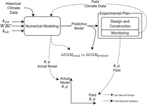
Figure 1. Design-validation mind map.
The 2nd step involved numerical modeling to predict the hydraulic behaviour and subsequent design of the experimental plan. The software chosen (HYDRUS 2D; PC-Progress) is industry recognized for modeling unsaturated water flow. This software allows for optimal management of boundary conditions that best simulate field conditions, in particular, the atmospheric interface and seepage face below the MOL. The objective of this step is to determine LUGM for different slopes, based on laboratory-determined occlusion values (water content). For research purposes, we opted for a design which forces LUGM to occur within the biofilter, so that we can verify the accuracy of its prediction (4th step). In this case, we arbitrarily decided to place the design LUGM at about ¾ of the length of the biofilter, herein denominated Target LUGM. This means that ¼ of the interface would become obstructed.
The 3rd step in the design process was the construction, instrumentation, and monitoring of the experimental MOB, presented by Nelson et al. (2022). The 4th and last design step was the validation, which aimed at providing an objective assessment of the proposed design methodology. This validation is fundamental because, ultimately, MOB end-users will have to rely on predictive modeling only (2nd step). Validation starts by assessing if LUGM (based on field water content values) is attained at the Target LUGM (or design point), obtained in the 2nd design step, therefore from modeling runs using historical climate data.
One occlusion criterion to determine LUGM that was initially considered was volumetric water content, θ, greater than θw-occ for more than 3 consecutive days. This is a valid way to address this assessment, in particular, because it excludes long periods of heavy rainfall. However, we decided to consider various water content percentiles to determine LUGM. For example, the 95% percentile means that only 5% of the values—the highest ones—were excluded from the analysis, and, therefore, from determination of LUGM. The subsequent step in the validation process was to compare field water content and suction values at specific points with values obtained from model runs using field climate data. Verification took place on a day-by-day basis. In addition, LUGM values obtained from the second modeling run (using field climate data) were compared with LUGM values obtained from the predictive model (using historic climate data).
3 Media characterization
As noted by van Verseveld and Gebert (2020), increasing air-filled porosity is essential for increasing permeability and allowing methanotrophic bacteria to access oxygen. The MOL material consisted of a mixture of two parts compost with one part plastic pellets (by volume), herein denominated compost mix (Figure in Table 1, left). The pellets were added to provide structure, increasing total porosity. The compost was sourced from the Region of Waterloo composting facility in Cambridge, Canada, out of unsieved compost basically composed of leaves, leftover food, and branches. Non-compostable matter (such as plastic residue) could be found in the raw compost. The unsieved nature of this material yields a highly heterogeneous structure. The plastic pellets are a mixture of resin manufactured from post-consumer materials in Canada.
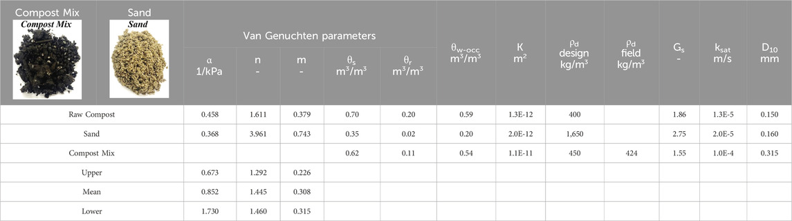
Table 1. Material properties.
The upper part of the GDL was composed of sand (Figure in Table 1, right). The sand is used as a filter material to prevent particles from migrating from the MOL to the GDL. The sand was provided by a local aggregate material supplier. Its characterization was crucial because a capillary barrier was expected to occur at the interface between the compost mix (MOL) and the sand filter layer. Table 1 summarizes all the relevant characterization parameters of the 1st step of the design-validation methodology (Figure 1).
The water retention curve (WRC) was obtained from laboratory testing data using the van Genuchten (1980) formulation. We used both a commercial apparatus and a customized test cell and methodology to obtain the WRC data points. The WRC of the sand, presented in Figure 2A, was obtained using the Hyprop device (Meter Group, 2015). The saturation water content of the sand, which may appear high, is explained by the very low density of the test samples (Table 1; Eq. 2).
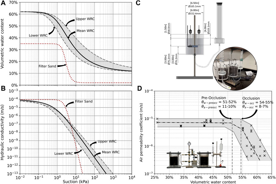
Figure 2. Water retention curve (A), hydraulic conductivity function (B), apparatus to obtain the latter two (C) and air permeability function (D) of the materials.
Despite its simplicity, the use of Hyprop for compost mixes may be impossible when large structural particles are present, as was the case here. We therefore adopted a similar testing principle, but in a cell that we designed. Figure 2C shows the cell designed to obtain the WRC of the compost mix. The internal diameter of the cell is 152.4 mm (i.e., the same as the height of the sample). It is designed to allow saturation from the bottom using a Mariotte bottle, therefore under constant head. This enables air bubbles in the sample to be expelled more efficiently, speeding up the saturation process. The cell is instrumented at mid-height with an EC-5 water content probe (manufactured by Meter Group), using the following custom calibration specific to the material (Eq. 1), where RAW is the raw sensor reading:
This EC-5 was chosen for its small radius of influence—estimated at 80 mm (Meter Group, 2021a) –, thereby avoiding border effects. To measure suction, Teros 31 tensiometers (Meter Group, 2022) were also installed at mid-height. Two identical cells have been manufactured so that tests can always be carried out in duplicate.
The resulting WRC is comparable with that obtained by Rüth et al. (2007). Due to heterogeneity of materials, the WRC for the compost mix varied substantially from one sample to another. Accordingly, in Figure 2A, rather than a single curve, we present an envelope of WRCs. The upper WRC is at the upper boundary of the envelope, the lower WRC at the lower boundary, while the mean WRC is the average suction value for a given water content for all eight samples. The saturated water content (θs) is assumed equal to the total porosity and is calculated using Eq. 2, where ρd is the dry density, Gs the specific density of the sample (see Table 1), and ρw the density of water.
Figure 2A presents the WRC of the chosen materials and Figure 2B the hydraulic conductivity functions (kfct) derived from their respective WRC. We adopted the transformation model proposed by van Genuchten (1980) using the k-function formulated by Mualem (1976).
The intrinsic permeability (K; L2) and water content at occlusion (θw-occ) were obtained via the air permeability function (kair-fct) in an air permeameter. The dry density for design (ρd-design) was obtained via static compaction in a proctor mould, an approach similar to preparing samples to be tested in an oedometer. This is used as the target self-weight for laboratory testing. The field dry density (ρd-field) was the density in the field after 1 year obtained following the ASTM-D 2167 Rubber Balloon Standard (ASTM, 2016). Gs, the specific density, was obtained by saturating the sample at low density in a rigid-wall permeameter (therefore not according to standard, because of the nature of compost-rich materials, which float in water). Due to the challenge of achieving saturation of a compost-rich mixture through conventional means, a variety of techniques were employed to determine the saturated hydraulic conductivity (Ksat). Table 2 presents the average values from several laboratory tests.
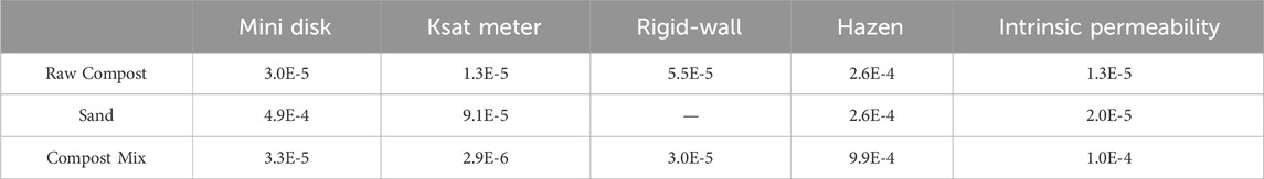
Table 2. Saturated hydraulic conductivity (m/s).
Due to its simplicity, the MiniDisk infiltrometer (Meter Group, 2021b), designed for field measurements, was systematically applied to all soil samples studied. Results obtained from this apparatus were calculated based on van Genuchten (1980) parameters and were used for comparative analysis. For sand, reference values from the user manual were employed, while for compost, the measured α and n values were used. In the case of the compost mix, the mean value was applied. Values obtained using the KSAT device (Meter Group, 2017) were included in the table, but due to the apparatus cells’ incompatibility with larger-scale structural materials, such as wood chips, also found in the compost mix, these values are not considered reliable.
The rigid-wall permeameter was additionally employed, as it enabled material saturation under pressure, addressing the above-mentioned challenge in saturating compost-based mixes. Nonetheless, the heterogeneity of the compost mix led to significant variability in results. Among the 27 permeability measurements taken from 8 distinct samples, values ranged from 2.2E-6 to 1.5E-4 m/s. Hazen’s equation is widely accepted for estimating permeability in sand. Since the D10 value of compost is comparable to that of sand, Hazen’s equation was used for comparison purposes.
K, a constant for a material, was determined by means of air permeability tests (described hereafter). These measurements yielded stable values since it was easier to circulate air than water through the mix. K allows for easy determination of the saturated permeability using ρw ≈ 1,000 kg.m−3, the gravitational acceleration (g = 9.81 m.s−2) and the dynamic viscosity (μ ≈ 0.001 Pa.s) according to Eq. 3. Given the stability of the intrinsic permeability, we decided to employ it in the MOB design process.
The kair-fct, presented in Figure 2D, was also carried out in a cell that we designed, to accommodate large particles from the compost mix. This cell has an internal diameter of 19 cm, and the height of the sample is 18 cm. Pressure is controlled by a pressure gauge at the inlet (bottom) and the flow rate is measured at the outlet (top) using a soap bubble gas flow meter (Bubble-O-Meter). The methodology and calculations are explained by Ahoughalandari et al. (2018). Two identical cells were manufactured so that the tests could always be carried out in duplicate.
The kair-fct is characterized by two sections. In the first, the air permeability remains nearly constant with increasing water content. The second section starts when the occlusion water content (θw-occ) is reached. At this point, air permeability drops drastically with the increasing water content. This occurs when air-filled pore voids are no longer interconnected, sharply reducing its diffusivity. In certain cases, as observed by Ahoughalandari et al. (2018), there is a third section between the other two. It starts when what can be denominated the pre-occlusion point is reached at θw-preocc. Gas flow is reduced, but there may still be a few interconnected pores. As a consequence, the drop in kair is not as drastic as when θ > θw-occ.
In Figure 2D, we can see that the plateau obtained for the compost mix is relatively well defined up to θw-preocc of 51%–52%. Due to the heterogeneity of the material, as well as the hydrophobicity of the plastic pellets used as a structuring agent, it was difficult to control the water content between θw-occ and θw-preocc, resulting in a gap between these two water content values. The adopted value for θw-preocc was set at 52%. When θ > θw-occ ≈ 54%–55%, there is a clear drop in air permeability. It is not possible to have a very precise value due to the heterogeneity of the mix, i.e., the drop does not always occur at the same spot. To adopt a conservative design value, we set θw-occ at 54%. For design purposes, Ahoughalandari et al. (2018) suggested using a conservative value, therefore adopting occlusion when θ ≈ θw-preocc.
4 Predictive design modeling parameters
The objective of the 2nd step in the design-validation methodology (Figure 1) is to predict the flow of water in the MOB, and the optimization of LUGM. Preliminary models showed that a total length of 10 m would allow LUGM to occur within the length of the MOB. In addition, due to space limitations, the maximum length of the MOB had to be less than 10 m. For the purpose of validation, the Target LUGM for this study was set at 7.5 m from the upslope end of the biofilter (3/4 of the length of the biofilter).
Figure 3 shows the conceptualization of the numerical model. It shows the methane oxidation layer (MOL), which rests on a layer of filter sand above the GDL. The coarse nature of the GDL (gravel) allows incoming biogas to be distributed as uniformly as possible at the base of the MOL. Figure 3 also depicts the perforated tube that carries the biogas to the bottom of the biosystem. The red arrows show the theoretical path of the biogas through the MOL, a flow that is diverted into the zone where there is no pore occlusion, defined by LUGM. Water is drained via the p-trap. Water was supplied to the system by an atmospheric boundary condition. ECCC historic climatic data, shown in Figure 4, were applied. A line of observation points spaced 0.5 m apart was placed at the base of the MOL, 3 cm above the GDL-MOL interface (not shown in Figure 3).
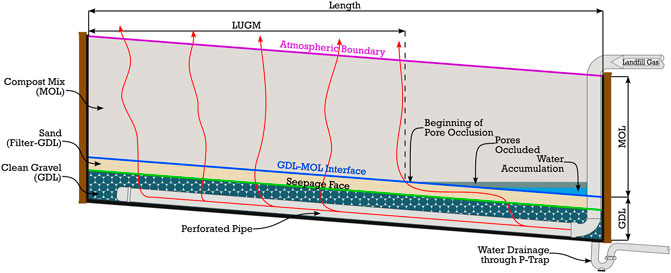
Figure 3. Schematic view of a biofilter with modeling boundaries.
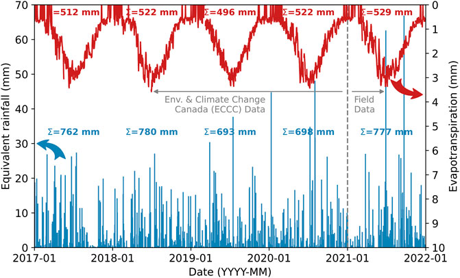
Figure 4. Climate data.
For numerical modeling purposes, only the compost mix and sand layers were incorporated in the model. In the model, an initial volumetric water content equal to 35% was applied to the compost and 25% to the sand. These values are the rounded average of the natural water content values taken from several samples delivered to the lab. A seepage face boundary condition was imposed at the interface between sand and gravel. The replacement of a layer by a seepage face is achieved by applying a trigger suction value. When this value is attained, drainage occurs. We assumed—for simplicity and to be conservative—that the clean gravel would not develop any suction, thus a nil suction (ψ = 0) was applied to the seepage face. As observed by McCartney and Zornberg (2010), and Kahale and Cabral (2022), in the field, the trigger suction value could be taken at the point of intersection of the kfct of the two materials.
The impact of width was assumed to be negligible (for hydraulic purposes) since the main direction of water flow is toward the downstream edge. For this study, the slope was varied from 0% to 8%, with an increment of 2%. The thickness of the MOB was set at 1 m, an effective thickness for methane oxidation (Roncato and Cabral, 2012). At this stage, consideration of oxidation capacity has not yet been optimally integrated, therefore we decided to adopt an arbitrary thickness value from the existing literature.
The meshing and convergence parameters were chosen to focus on the capillary barrier effect. The general mesh was set to triangles with a size of 100 mm, therefore the global precision offered is 1 kPa (P = ρgh, where “h” is the size of the mesh element). However, 1 kPa is not precise enough for the WRC of the compost mix since the saturation plateau ends well before 1 kPa (Figure 2A). A mesh refinement was therefore inserted at the GDL-MOL interface, with a size of 10 mm, thus a precision of 0.1 kPa. Finally, water content convergence was fixed at 0.1% and pressure convergence at 10 mm, thus 0.1 kPa.
Figure 4 shows the climate data applied at the atmospheric boundary condition of the models, both for the predictive models (2nd design step) with historical data from 2017 to 2020 and for the actual models (4th design step), with actual data measured from an on-site weather station in 2021. The historical climate data used to design the MOB were extracted from Environment and Climate Change Canada (2021) for the period considered for the design, i.e., 2017 to 2020. Precipitation values from direct measurement are shown in blue at the bottom of the figure, with the annual sum in the centre. Potential evapotranspiration, in red at the top of the figure, was calculated using the Oudin et al. (2005) method, while actual evapotranspiration was estimated using a linear calibration proposed by Amani et al. (2022). The annual sum (Σ) is shown at the top of the figure. The mean actual evapotranspiration, estimated at 516 mm annually, is consistent with what is considered as average for the Great Lakes region, i.e., 500–600 mm (Wang et al., 2013; Statistics Canada, 2017). For modeling purposes, precipitation as water in Figure 4 includes snowmelt during colder months, because the heat trace wire below the MOL caused snow to melt. Temperature profiles of the MOB presented by Nelson et al. (2022) confirmed that the MOB never froze. Finally, it is important to note the increase in heavy rainfall events over time. This is further reason for using the field climatic data in numerical modeling when comparing the response of the model with field response during the validation phase (4th step).
5 Design of the experimental plan
Following modeling, the next phase in the 2nd design step involved analyzing modeling data to choose a design which would meet the established criteria (LUGM ≈ 7.5 m), and then preparing the plans and specifications for the construction of the experimental biosystem. For this step, 12 models were considered, out of the 153 initially attempted. The main reason for this high number of initial models was testing the sensitivity of certain parameters, such as the trigger suction on seepage faces, and choice of kfct (Table 2). Non-convergence of certain models also was an issue.
The density distribution panes in Figure 5 show the frequency of occurrence of water content values, rounded to the nearest 0.1%. Only the upper WRC is shown, given the fact that it represents the worst-case scenario (highest water content for the same suction). The 4-year frequency scale, produced with historical climate data (Figure 4—2017–2020), is the same for all the panes. Each curve represents the distribution of water content for each of the points along the interface for the 0%, 2%, 4%, 6% and 8% slope models, from top to bottom. The curves are represented by the colour (blue to yellow) associated with their respective observation point located along the GDL-MOL interface (Figure 3) number (1–19) spaced every 0.5 m, as shown in the insert in the top left-hand corner. The emphasis is on points 1 (closest point to downstream edge), 5 (Target LUGM = 7.5 m from upstream) and 19 (closest point to upstream edge). The curves associated with these three points are represented by bold dotted distribution contours. A zone is considered unoccluded when the water content is lower than θw-preocc, while the MOB is occluded when the water content is greater than θw-occ. The pre-occlusion range lies between these two values.
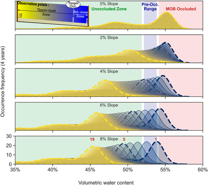
Figure 5. Water content occurrence frequency using the upper WRC model. Scale repeats for every subplot (magnitude depends on the number of years analyzed). Numbers relate to observation points in the predictive numerical models adopted for design purposes. The observation points are located along the GDL-MOL interface.
The results presented in Figure 5 show the impact of slope on the hydraulic behaviour of the MOB. The greater the slope, the greater the length of the unoccluded zone. There is a noteworthy difference from the flat (0% slope) model to the 4% sloped model. However, the effect of slope decreases for slopes greater than 4%, particularly when the biofilter is drier (e.g., values related to observation point 19 remain relatively stable). Models with 6% and 8% slopes show a similar behaviour. However, there is a shift to the left for the downstream points (e.g., observation point 5), meaning that the biofilter becomes drier—or, at least, less occluded, downstream, with higher slopes. An 8% slope was eventually adopted for construction because of this slight shift towards the left for point 5. At 8%, slope points 1 to 4 (0.5–2 m) have a tail in the MOB occluded zone, whereas point 5 does not.
Figure 6 presents the water content distributions shown in Figure 5 transformed into a single design criterion: LUGM. Slopes equal to 0%, 4%, 6% and 8% are shown for the upper WRC (green), mean WRC (orange), and lower WRC (purple). For clarity of the presentation, the 2% slope was excluded from this figure. This transformation shows the maximum water content at each observation point as a function of their location along the interface. The beginning of the X-axis is the upstream edge, and 10 m is the downstream edge of the MOB.
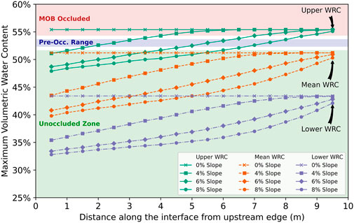
Figure 6. LUGM obtained with the predictive numerical models. Slopes are shown for the upper WRC (green), mean WRC (orange), and lower WRC (purple).
The upper WRC and the mean WRC are always in the unoccluded zone. Models using the upper WRC are occluded for the most part at the 0% and 4% slopes. At a 6% slope, the maximum water content is on both sides of the pre-occ zone. We only find the majority of the water content values in the unoccluded zone when considering an 8% slope. The design criterion LUGM = 7.5 m is met for the 8% slope, when adopting the upper WRC. The pre-occ range extends from 6.5 to 8.5 m, also justifying the 8% slope adopted for construction purposes. Finally, this analysis shows that the WRC has a significant impact on the value of LUGM. Proper determination of the WRC in the laboratory is therefore of the utmost importance. A slight deviation in the WRC (Figure 2A) could substantially alter the design. Table 3 shows a summary of LUGM values for each of the selected models, this time including all 3 WRCs.
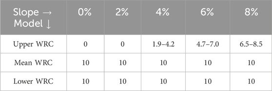
Table 3. Selected LUGM values (in meters) as a function of slope and model.
Maximum water content as a function of position is used as the design criterion since it is hard to determine a unique value from the density distribution (Figure 5). The maximum water content gives the shortest LUGM, which provides a design for the worst-case scenario. It is debatable whether it would not be better to use a probability distribution criterion allowing a certain percentage of the time occluded, thus the presentation of the temporal variation of the LUGM shown in Figure 7.
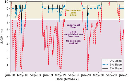
Figure 7. Temporal variation of LUGM obtained with the upper WRC model.
Figure 5 presented the range of possible water content values in the MOB, while Figure 6 (and the summary in Table 3) presented the worst-case scenario for LUGM. Figure 7 presents the temporal variation of LUGM over the 4 years of preliminary modeling. Occlusion above Target LUGM is identifiable by the segments where the LUGM is below the white line (LUGM = 7.5 m). It can be observed that designs using the upper WRC and 6% or 8% slopes meet the design criteria. The 2% slope was also plotted to show—to the extreme—the impact of seasonality on the hydraulic response of the MOB. Indeed, one can see that for a 2% slope, the biofilter is very dry during summer (June to September), and would work very well, since LUGM would be greater or equal to 10 m. However, during winter, the 2% sloped MOB would be occluded all the time, with the exception of two spikes.
This observation opens the debate on the design criterion. Is it preferable to design a system using the maximum water content to identify the LUGM (in order to have a system that is functional at all times) or to design a system using a probability distribution criterion, (even if it means accepting short non-functional periods)? The authors believe that this criterion is at the discretion of the MOB designer, depending on the level of risk accepted for each project.
This 2nd step of the design-validation methodology determines the design parameters enabling construction of a full-scale experimental plan to validate the design hypotheses.
6 Construction and installation of monitoring equipment
Construction details, choice of instrumentation and monitoring details (3rd step in the validation process) are explained in Nelson et al. (2022). Figure 8 shows a sectional view and the dimensions of the constructed MOB at the Old Kitchener landfill. The length of the biofilter was set at 10 m, its width at 3 m and the slope at 8%. The thicknesses of the MOL and sand layer were 1 m and 0.15 m, respectively.
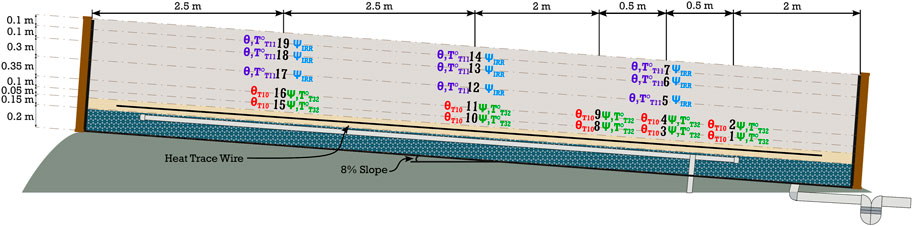
Figure 8. Constructed biofilter. Numbers relate to observation points in the numerical model adopted for field validation.
Volumetric water content sensors (identified as θ) and tensiometers (identified as ψ) probes were installed at the locations (observation points) shown in Figure 8, numbered 1 to 19. In this experimental plot, we used Teros 10 (identified as T10, in red) and Teros 11 (T11, in purple), water content sensors, both manufactured by Meter Group. Teros 11 probes were placed close to the surface to monitor temperature. Teros 32 tensiometers (T32, in green) were placed near the bottom interface, while Irrometer tensiometers (IRR, in blue) were placed near the surface. Observation points 1, 3, 8, 10 and 15 were placed along the GDL-MOL interface. Data from these observation points were used for design validation using Hydrus.
Additional probes were placed in the downstream area to closely monitor the occurrence of LUGM, therefore verify if it occurred at the expected occlusion point (target LUGM = 7.5 m from the upstream edge). The near-surface instrumentation helped validate the overall behaviour of the MOB.
7 Validation of initial design and methodology
This 4th step aimed at providing an objective assessment of the proposed design methodology. We started the validation process with a simple question: Was the field LUGM (determined based on field water content data) close enough to the target LUGM (determined from numerical model runs using historic climate data; 2nd step)?
Figure 9 presents field water content values along the GDL-MOL interface. These values are compared to occlusion and pre-occlusion water content values obtained from the laboratory (Figure 2D). We subdivided the biofilter into three zones, namely, the occluded, the pre-occluded, and the unoccluded (gas is free to flow) zones. If all the field water content values are considered (100th percentile), the pre-occluded zone would start at ∼ 4 m. However, if values logged after major precipitation events are excluded, thereby excluding the 5% highest values (95th percentile) or the 10% highest (90th percentile) values, occlusion occurs at approximately the target value (7.5 m). The dent shown in Figure 9 results from a problem with the probe placed 7.5 m away from the upstream edge, along the interface. This sensor stopped working on 12 September 2021, and the highest water content for sensors placed at 5 m, 7 m and 8 m occurred in mid-September 2021, i.e., after the sensor at 7.5 m stopped working.
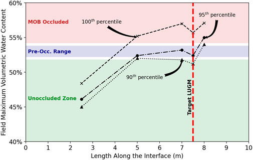
Figure 9. State of occlusion along the GDL-MOL interface based on field data. The biofilter was subdivided into three following zones: occluded, pre-occluded, and unoccluded.
The results in Figure 9 show that if major precipitation events are excluded (i.e., using the 95th or 90th percentiles), the target LUGM is attained. Behaviour of real (Figure 9) and modeled MOB (8% slope, upper WRC; Figure 6) match reasonably by excluding the 5% highest water content values in the field. This exclusion seems valid from the engineering design perspective, in the sense that the designer would accept a malfunction of the MOB for short periods of time. The impact of extreme precipitation on water content values along the interface can also be observed in Figure 7.
Figure 10 is analogous to Figure 7, and shows the evolution of LUGM values in the biofilter during the field study period. The main difference here is that we have divided this figure into two sections. For both upper and lower panes, the position of LUGM is represented by the x symbols on the dotted lines, i.e., it indicates where θw > θw-occ. The bold dotted red line represents the Target LUGM (7.5 m). The violet zones on the top and bottom panels represent the locations where instruments were placed (Figure 8). The jumps in LUGM values reflect the non-continuous positioning of sensors placed along the interface (Figure 8). If LUGM values lie either before the first sensor or beyond the farthest one from the upstream edge, no point or line is plotted. At the bottom of each pane is the equivalent rainfall, which considers total precipitation as water (Figure 4), including snowmelt.
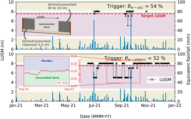
Figure 10. Temporal variation of LUGM based on field data.
The upper panel in Figure 10 presents the evolution of the length of unrestricted gas migration considering θw-occ = 54%. It can be observed that the target LUGM is exceeded (values below the Target value) during—or following—extreme rainfall events (e.g., July and September). With respect to free gas migration across the GDL-MOL interface, it is reasonable to state that the designed MOB worked quite well when considering θw-occ = 54%. This was not the case when θw-occ = 52% (results in the lower panel). In this case, LUGM exceeded the Target value rather often, reaching values as low as 5 m for long periods of time (e.g., early July and early September), meaning that the design would not have met expectations. An insert in the lower panel shows the raw water content data over time for the period when the MOB did not work properly (assuming θw-occ = 52%). This insert shows that the probe located at 5 m (in red) oscillated immediately above and below the pre-occlusion line (52%) throughout the summer. This shows the risk and sensitivity of this type of design which makes the case for proper laboratory testing and careful analysis of the results when selecting an occlusion activation function, as does the difference in behaviour between the two scenarios (θw-occ = 54% or 52%).
In the next exercise of the validation process, field climate data were fed into the numerical model, so that the model was exposed to site-specific climatic variations. We then compared field moisture content and suction values at observation points with values determined from numerical model runs using field climate data. This way, any discrepancy between model values (with actual weather data) and field water content values could be attributed to other parameters, such as the adopted WRC.
The heatmaps in Figure 11 show the daily difference between water content values obtained from numerical modeling using field climatic data (θmodel) and measured in the field (θfield). Figure 11A shows this difference at the GDL-MOL interface, i.e., at a depth of 0.95 m (Figure 8), while Figure 11B shows this difference 10 cm above the interface (0.85 m deep). The points are numbered, for each model, incrementing from downstream (point 1 at the interface and point 2 just 10 cm above point 1; Figure 8) to upstream (point 15 at the interface and point 16 at 10 cm above). Differences are presented on a scale of −0.20 to 0.20 in volumetric water content. The scale was flattened to 16 colours to enhance visual differentiation. Each heatmap is divided into three sections, one for each of the three different WRC models used during the design phase, namely, the upper, mean, and lower water retention curves (Figure 2A). Light-shaded areas represent a perfect match, meaning that the numerical model has predicted the actual hydraulic behaviour, whereas dark-shaded areas mean that the numerical model has not predicted the actual hydraulic behaviour. The darker the area, the greater the difference. Grey shaded zones represent unavailable data. Blue represents an underestimation of water content values (field greater than model), while red-shaded pixels mean an overestimation of water content values (model greater than field).
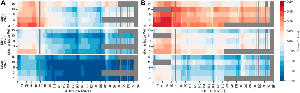
Figure 11. Difference in water content values obtained from the numerical model and the field, considering the upper, mean and lower WRCs. At the GDL-MOL interface (A) and 5 cm above this interface (B). Instrumentation points are indicated in Figure 8.
At the interface (Figure 11A), the lower WRC underestimates water content values, thus the dark blue pixels. The mean WRC also underestimates water content values, but not as much, leading to slightly lighter pixels. The upper WRC underestimates field values in the beginning (probably initial wetting of the organic matter in the compost mix) but estimates water content values rather well (mostly lighter pixels). The results in Figure 11B (10 cm above the interface), show that the upper WRC clearly overestimates θfield. The mean WRC slightly overestimates θfield, while the lower WRC tends to underestimate it. The optimal WRC would lie between the mean and lower WRC, as discussed next.
In an additional validation exercise, we compared the water retention curves obtained in the laboratory (used for design purposes; Figure 2A) with data points obtained from tensiometers placed very close to water content sensors. In Figure 12, only the suction and water content values obtained from the instrumentation points near the GDL-MOL interface (red squares) and 10 cm above it (blue dots) were plotted. They fall within two relatively dense clusters: one for the interface and another for the region just above it. In both cases, the MOL never became too wet or too dry.
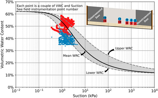
Figure 12. Restitution of the field water retention curve. Numbers relate to observation nodes in the numerical model adopted for field validation.
Interface points (in red) tend to be close to the upper WRC, while above the interface (blue), they tend to lie between the mean and lower WRCs, as observed previously. Despite the fact that there are a seemingly large number of blue points under the lower WRC, they only number 182, which is a fraction of the 3,452 points located over or above the lower WRC. For this analysis, we excluded a small number of suction values logged right after tensiometer resaturation, when suction values become nil or even positive (pressure). Figure 12 reconfirms the assertion made previously that the actual WRC representing the region above the interface would lie between the lower and mean WRCs.
The observed behaviour for this particular MOB seems to indicate that the design of MOBs constructed with organic-rich materials such as compost might be perfected by working with an envelope of WRCs, instead of fitting a unique curve from laboratory points. This would make it possible to assign different WRCs for the region very close to the interface and another WRC for the rest of the MOL above the interface. Unpublished data from another experimental site monitored by the same authors and other colleagues—also built using organic matter—also indicate that the design of MOBs constructed with organic-rich materials such as compost might be perfected by working with an envelope of WRCs. Further field studies, based on observation of experimental MOBs (particularly those properly instrumented), will shed more light on this subject. Field studies may also help further validate the hypothesis that MOB designers can rely solely on numerical modeling based on historic climatic data.
8 Conclusion
In this study we validated the prediction of the hydraulic response of an experimental MOB using numerical modeling and field data. We analyzed the evolution of moisture at the interface between the GDL and MOL. The magnitude of the length of unrestricted gas migration (LUGM) depended on the level of occlusion of the pore voids. Through experimental evidence, it was established that θw-occ was a suitable activation function to define occlusion, therefore LUGM. The results of these experiments led to the conclusion that accurate modeling of MOB hydraulic behavior and determination of LUGM is possible using laboratory-derived hydraulic and geotechnical parameters. The main contribution of this study lies in a confirmed validation of the design methodology through modelling using field measurements (suction, water content) and real climatic data.
Bearing in mind that designers will only be relying on numerical models (physical models are mainly the domain of researchers) an important question needed to be answered, i.e., is it possible to rely on numerical modeling for the design of MOB? The results presented herein seem to indicate that the answer is a sound yes, if one follows the design methodology proposed herein, based on numerical modeling with proper soils and climatic data, plus appropriate boundary conditions (and a good dose of common sense, as usual). Further on-going field studies will allow more comparisons between physical and numerically modelled behaviour of MOBs.
Noteworthy observations revealed different behaviours of the MOL material at the GDL-MOL interface and right above it. The prospect of specifying distinct Water Retention Curves (WRCs) for the same material may lead to improved designs using numerical modeling. For this purpose, additional properly instrumented MOB field studies would be necessary, in which MOL and GDL materials would be thoroughly characterized.
Water generated by methanotrophic activity was not considered during modeling. The following improvement strategies could be adopted: 1. Estimate the amount of liquid water produced in the laboratory, while submitting samples to conditions as similar as possible to those in the field. A simplified approach (to be tested) would be to simply add the amount of liquid water generated to the net infiltration (precipitation minus evaporation). 2. Carry out a mass balance of infiltration water and water recovered from the bottom drain. We could not quantify the impact of these limitations in this study.
Data availability statement
The original contributions presented in the study are publicly available. This data can be found here: https://github.com/geoenvironnement/validation-of-a-methane-oxidation-biofilter-design-methodology-using-numerical-modeling.
Author contributions
YD: Conceptualization, Data curation, Formal Analysis, Investigation, Methodology, Validation, Writing–original draft. BN: Investigation, Methodology, Writing–review and editing. RZ: Supervision, Writing–review and editing. AC: Supervision, Conceptualization, Funding acquisition, Investigation, Methodology, Project administration, Validation, Writing–original draft.
Funding
The authors declare that financial support was received for the research, authorship, and/or publication of this article. The work presented in this paper received financial support from NSERC (ALLRP 548667-19), Dillon Consulting Ltd. and the Regional Municipality of Waterloo.
Acknowledgments
The authors also acknowledge the contribution of several members of the BiomethoxUS Group (Université de Sherbrooke) and from personnel from the University of Guelph.
Conflict of interest
Author BN was employed by Dillon Consulting Ltd., after completion of the data acquisition phase.
The remaining authors declare that the research was conducted in the absence of any commercial or financial relationships that could be construed as a potential conflict of interest.
Publisher’s note
All claims expressed in this article are solely those of the authors and do not necessarily represent those of their affiliated organizations, or those of the publisher, the editors and the reviewers. Any product that may be evaluated in this article, or claim that may be made by its manufacturer, is not guaranteed or endorsed by the publisher.
References
Ahoughalandari, B., and Cabral, A. R. (2017a). Landfill gas distribution at the base of passive methane oxidation biosystems: transient state analysis of several configurations. Waste Manag. 69, 298–314. doi:10.1016/j.wasman.2017.08.027
Ahoughalandari, B., and Cabral, A. R. (2017b). Influence of capillary barrier effect on biogas distribution at the base of passive methane oxidation biosystems: parametric study. Waste Manag. 63, 172–187. doi:10.1016/j.wasman.2016.11.026
Ahoughalandari, B., Cabral, A. R., and Leroueil, S. (2018). Elements of design of passive methane oxidation biosystems: fundamental and practical considerations about compaction and hydraulic characteristics on biogas migration. Geotech. Geol. Eng. 36, 2593–2609. doi:10.1007/s10706-018-0485-z
Amani, A., Boucher, M.-A., Cabral, A. R., and Nadeau, D. F. (2022). “Assessing the generalization power of three machine learning models and three evapotranspiration formulas using 143 FLUXNET towers data,” in Presented at the EGU general assembly (Vienna, Austria: GU General Assembly). doi:10.5194/egusphere-egu22-5580
ASTM (2016). Standard test method for density and unit weight of soil in place by the rubber Balloon method. doi:10.1520/D2167-15
Cabral, A. R., Capanema, M. A., Gebert, J., Moreira, J. F., and Jugnia, L. B. (2010a). Quantifying microbial methane oxidation efficiencies in two experimental landfill biocovers using stable isotopes. Water. Air. Soil Pollut. 209, 157–172. doi:10.1007/s11270-009-0188-4
Cabral, A. R., Létourneau, M., McCartney, J. S., Parks, J., Yanful, E., and Song, Q. (2010b). “Geotechnical issues in the design and construction of PMOBs,” in Unsaturated soils (London, England: Taylor and Francis Group), 7.
Capanema, M. A., Cabana, H., and Cabral, A. R. (2014). Reduction of odours in pilot-scale landfill biocovers. Waste Manag. 34, 770–779. doi:10.1016/j.wasman.2014.01.016
Capanema, M. A., and Cabral, A. R. (2012). Evaluating methane oxidation efficiencies in experimental landfill biocovers by mass balance and carbon stable isotopes. Water. Air. Soil Pollut. 223, 5623–5635. doi:10.1007/s11270-012-1302-6
Capanema, M. A., Ndanga, E., Lakhouit, A., and Cabral, A. R. (2013) Methane oxidation efficiencies of A 6-year-old experimental landfill biocover. in Fourteenth International Waste Management and Landfill Symposium. Cagliari, Italy.
Cassini, F., Scheutz, C., Skov, B. H., Mou, Z., and Kjeldsen, P. (2017). Mitigation of methane emissions in a pilot-scale biocover system at the AV Miljø Landfill, Denmark: 1. System design and gas distribution. Waste Manag. 63, 213–225. doi:10.1016/j.wasman.2017.01.013
Environment and Climate Change Canada (2021). Historical climate data. Past Weather Clim. Available at: https://climate.weather.gc.ca/.
Fjelsted, L., Scheutz, C., Christensen, A. G., Larsen, J. E., and Kjeldsen, P. (2020). Biofiltration of diluted landfill gas in an active loaded open-bed compost filter. Waste Manag. 103, 1–11. doi:10.1016/j.wasman.2019.12.005
Gebert, J., and Groengroeft, A. (2006). Performance of a passively vented field-scale biofilter for the microbial oxidation of landfill methane. Waste Manag. 26, 399–407. doi:10.1016/j.wasman.2005.11.007
Gebert, J., Groengroeft, A., and Pfeiffer, E.-M. (2011). Relevance of soil physical properties for the microbial oxidation of methane in landfill covers. Soil Biol. biochem. 43, 1759–1767. doi:10.1016/j.soilbio.2010.07.004
Gebert, J., Huber-Humer, M., and Cabral, A. R. (2022). Design of microbial methane oxidation systems for landfills. Front. Environ. Sci. 10, 907562. doi:10.3389/fenvs.2022.907562
Huber-Humer, M., Gebert, J., and Hilger, H. (2008). Biotic systems to mitigate landfill methane emissions. Waste Manag. Res. 26, 33–46. doi:10.1177/0734242X07087977
Humer, M., and Lechner, P. (1999). Alternative approach to the elimination of greenhouse gases from Old landfills. Waste Manag. Res. 17, 443–452. doi:10.1034/j.1399-3070.1999.00064.x
Jugnia, L.-B., Cabral, A. R., and Greer, C. W. (2008). Biotic methane oxidation within an instrumented experimental landfill cover. Ecol. Eng. 33, 102–109. doi:10.1016/j.ecoleng.2008.02.003
Kahale, T., and Cabral, A. R. (2022). Field and numerical evaluation of breakthrough suction effects in lysimeter design. Environ. Technol. 45, 1169–1182. doi:10.1080/09593330.2022.2139635
Kahale, T., Ouédraogo, O., Duarte Neto, M., Simard, V., and Cabral, A. R. (2022). Field-based assessment of the design of lysimeters for landfill final cover seepage control. J. Air Waste Manag. Assoc. 72, 1477–1488. doi:10.1080/10962247.2022.2126557
Kaza, S., Yao, L., Bhada-Tata, P., Van Woerden, F., lonkova, K., Morton, J., et al. (2018). What a waste 2.0: a global snapshot of solid waste management to 2050, Urban development series. Washington, DC, USA: World Bank Group.
Lacroix Vachon, B., Abdolahzadeh, A. M., and Cabral, A. R. (2015). Predicting the diversion length of capillary barriers using steady state and transient state numerical modeling: case study of the Saint-Tite-des-Caps landfill final cover. Can. Geotech. J. 52, 2141–2148. doi:10.1139/cgj-2014-0353
McCartney, J. S., and Zornberg, J. G. (2010). Effects of infiltration and evaporation on geosynthetic capillary barrier performance. Can. Geotech. J. 47, 1201–1213. doi:10.1139/T10-024
Mualem, Y. (1976). A new model for predicting the hydraulic conductivity of unsaturated porous media. Water Resour. Res. 12, 513–522. doi:10.1029/WR012i003p00513
Nelson, B., Zytner, R. G., Dulac, Y., and Cabral, A. R. (2022). Mitigating fugitive methane emissions from closed landfills: a pilot-scale field study. Sci. Total Environ. 851, 158351. doi:10.1016/j.scitotenv.2022.158351
Oudin, L., Hervieu, F., Michel, C., Perrin, C., Andréassian, V., Anctil, F., et al. (2005). Which potential evapotranspiration input for a lumped rainfall–runoff model? J. Hydrol. 303, 290–306. doi:10.1016/j.jhydrol.2004.08.026
Roncato, C. D. L., and Cabral, A. R. (2012). Evaluation of methane oxidation efficiency of two biocovers: field and laboratory results. J. Environ. Eng. 138, 164–173. doi:10.1061/(ASCE)EE.1943-7870.0000475
Rüth, B., Lennartz, B., and Kahle, P. (2007). Water regime of mechanical—biological pretreated waste materials under fast-growing trees. Waste Manag. Res. 25, 408–416. doi:10.1177/0734242X07076940
Scheutz, C., Cassini, F., De Schoenmaeker, J., and Kjeldsen, P. (2017). Mitigation of methane emissions in a pilot-scale biocover system at the AV Miljø Landfill, Denmark: 2. Methane oxidation. Waste Manag. 63, 203–212. doi:10.1016/j.wasman.2017.01.012
Scheutz, C., Fredenslund, A. M., Chanton, J., Pedersen, G. B., and Kjeldsen, P. (2011). Mitigation of methane emission from Fakse landfill using a biowindow system. Waste Manag. 31, 1018–1028. doi:10.1016/j.wasman.2011.01.024
Scheutz, C., Pedersen, R. B., Petersen, P. H., Jørgensen, J. H. B., Ucendo, I. M. B., Mønster, J. G., et al. (2014). Mitigation of methane emission from an Old unlined landfill in klintholm, Denmark using a passive biocover system. Waste Manag. 34, 1179–1190. doi:10.1016/j.wasman.2014.03.015
Statistics Canada (2017). Average annual evapotranspiration, 1981 to 2010. Available at: https://www150.statcan.gc.ca/n1/pub/16-201-x/2017000/sec-2/m-c/m-c-2.5-eng.htm.
van Genuchten, M.Th (1980). A closed-form equation for predicting the hydraulic conductivity of unsaturated soils. Soil Sci. Soc. Am. J. 44, 892–898. doi:10.2136/sssaj1980.03615995004400050002x
van Verseveld, C. J. W., and Gebert, J. (2020). Effect of compaction and soil moisture on the effective permeability of sands for use in methane oxidation systems. Waste Manag. 107, 44–53. doi:10.1016/j.wasman.2020.03.038
Wang, A., and J. Lee, J. (2022). Methane ‘super-emitters’ mapped by NASA’s new earth space mission. Available at: http://www.nasa.gov/feature/jpl/methane-super-emitters-mapped-by-nasa-s-new-earth-space-mission.
Keywords: design of methane oxidation biosystems, biofilter, unsaturated flow of water, water retention curve, length of unrestricted gas migration, capillary barrier, landfill cover
Citation: Dulac Y, Nelson BR, Zytner RG and Cabral AR (2024) Validation of a methane oxidation biosystem design methodology using numerical modeling. Front. Environ. Sci. 12:1397134. doi: 10.3389/fenvs.2024.1397134
Received: 06 March 2024; Accepted: 09 July 2024;
Published: 30 July 2024.
Edited by:
Marco Schiavon, University of Padua, ItalyReviewed by:
Song Feng, Fuzhou University, ChinaLuis Yermán, The University of Queensland, Australia
Copyright © 2024 Dulac, Nelson, Zytner and Cabral. This is an open-access article distributed under the terms of the Creative Commons Attribution License (CC BY). The use, distribution or reproduction in other forums is permitted, provided the original author(s) and the copyright owner(s) are credited and that the original publication in this journal is cited, in accordance with accepted academic practice. No use, distribution or reproduction is permitted which does not comply with these terms.
*Correspondence: Alexandre R. Cabral, YWxleGFuZHJlLmNhYnJhbEB1c2hlcmJyb29rZS5jYQ==