A methane monitoring station siting method based on WRF-STILT and genetic algorithm

Reducing methane emissions in the oil and gas industry is a top priority for the current international community in addressing climate change. Methane emissions from the energy sector exhibit strong temporal variability and ground monitoring networks can provide time-continuous measurements of methane concentrations, enabling the rapid detection of sudden methane leaks in the oil and gas industry. Therefore, identifying specific locations within oil fields to establish a cost-effective and reliable methane monitoring ground network is an urgent and significant task. In response to this challenge, this study proposes a technical workflow that, utilizing emission inventories, atmospheric transport models, and intelligent computing techniques, automatically determines the optimal locations for monitoring stations based on the input quantity of monitoring sites. This methodology can automatically and quantitatively assess the observational effectiveness of the monitoring network. The effectiveness of the proposed technical workflow is demonstrated using the Shengli Oilfield, the second-largest oil and gas extraction base in China, as a case study. We found that the Genetic Algorithm can help find the optimum locations effectively. Besides, the overall observation effectiveness grew from 1.7 to 5.6 when the number of site increased from 1 to 9. However, the growth decreased with the increasing site number. Such a technology can assist the oil and gas industry in better monitoring methane emissions resulting from oil and gas extraction.

1 Introduction

Methane emissions account for more than 10 per cent of China’s total greenhouse gas emissions, making it the second largest greenhouse gas after carbon dioxide (Omara et al., 2023). The radiative forcing of methane is greater than that of all other non-carbon dioxide greenhouse gases combined, and its global warming potential is over 80 times that of carbon dioxide over a 20-year period (Kirschke et al., 2013). In recent years, the atmospheric methane concentration has shown an accelerated growth trend, which has attracted great attention from the international climatology community (Jacob et al., 2016; Kang et al., 2016; Erland et al., 2022; Jacob et al., 2022; Peng et al., 2022). Reducing methane emissions associated with petroleum extraction is considered the most cost-effective pathway for methane reduction, and it also brings about economic benefits (Varon et al., 2019; Gong and Shi, 2021; Chen et al., 2022). Zhang et al., 2020 indicated a significant underestimation of oil and gas-related methane emissions in the Permian Basin of the United States. Irakulis-Loitxate et al., 2021 utilized high-resolution methane concentration anomaly inversion results from satellites such as PRISMA and GF-5 to identify prominent oil and gas methane emitters in the Permian Basin and quantified the emissions from these sources. D. J. Varon et al. used methane observation data from GHGSAT and TROPOMI to identify super-emitters of methane in the Central Asian oil fields. These smaller emission sources, though in smaller quantities, contribute to over 60% of the total emissions (Varon et al., 2018; Varon et al., 2019). Although high-resolution methane concentration anomalies have made significant progress in identifying and quantifying super-emitters of methane (Pei et al., 2023a), emissions from oil and gas sources exhibit notable temporality (Shi et al., 2022; Shi et al., 2023a). To accurately quantify their annual emissions, high-frequency concentration observations remain crucial (Chen et al., 2022; Schissel and Allen, 2022). Theoretically, TROPOMI’s XCH4 product offers a high observation frequency (Hu et al., 2018; Pei et al., 2020). However, studies have indicated interference from clouds and aerosols, preventing it from providing a sufficient frequency of observations in most regions of China (Zhang et al., 2022). Therefore, the establishment of ground-based monitoring networks plays an irreplaceable role in capturing the temporal variations in methane emission intensity from oilfields (Turner et al., 2016; Omara et al., 2023).

At present, China’s methane monitoring network is primarily utilized to reflect large-scale methane background concentrations (Wu et al., 2023), and a dedicated observational network for methane emissions monitoring has yet to be established. These two have fundamentally different design considerations. The former requires avoiding local emissions to better reflect large-scale fluxes (Laughner et al., 2023), while the latter needs to capture information about local emissions in order to quantify emission intensity (Tu et al., 2022). In 2021, under the supervision of the Ministry of Ecology and Environment of China, several Chinese cities initiated the construction of ground-based GHG monitoring networks to reflect the greenhouse gas fluxes in their respective urban areas (Sun et al., 2022; Zhang Y. et al., 2023). However, as of now, there have been no publicly available academic publications on the design methodology of such monitoring networks (Yang et al., 2024). In this work, we will introduce a method for selecting ground-based GHG monitoring site locations with the purpose of monitoring methane emissions from oilfields. In this study, we focus on the Shengli Oilfield, which is the second-largest oilfield in terms of petroleum production in China (Pei et al., 2023b; Shi et al., 2023b). In this study, we integrated TROPOMI’s XCH4 products to assess the reliability of two common oil and gas emission inventories, Global Fuel Exploitation Inventory (GFEI) and Emissions Database for Global Atmospheric Research (EDGAR), within our research area. Subsequently, using the Stochastic Time-Inverted Lagrangian Transport driven by Weather Research and Forecasting model (WRF-STILT) (Lin et al., 2003; Pei et al., 2022), we generated footprints for each monitoring site, stratified by wind speed, and rotated all footprints according to upwind conditions. Furthermore, we utilized ERA-5 reanalysis data (Liu et al., 2024) to establish probability distributions of wind speed and direction for each grid cell. Through these steps, we efficiently computed annual average footprints for every grid point across the entire study area. Ultimately, based on the principle of maximum methane concentration enhancement attributed to oilfield emissions and minimum enhancement from other sources, we formulated a quantified fitness function. This facilitated the optimization of site locations using a Genetic Algorithm (GA). This framework efficiently determines optimal site positions for varying site quantities, offering a relatively straightforward yet quantitatively characterized design strategy for greenhouse gas emission monitoring networks.

The remaining parts of this work are organized as follow. In Section 2, we describe the proposed optimization method for determining locations of monitoring site as well as the data and tools we used in this work. In Section 3, we demonstrate samples of footprints generated by WRF-STILT. Besides, we also present the optimization process and results of the proposed method in Shengli oilfield. In Section 4, we discuss the potential limitations of this method and directions for improvement. Finally, we summarize the whole work in Section 5.

2 Methodology and data

2.1 Quantitative metrics for a single observation site

To enhance the site selection process for the methane observation network, it is imperative to establish specific quantitative metrics that gauge the effectiveness of individual sites. In this study, we introduce the pivotal concept of “footprint,” extensively utilized in flux inversion, to precisely characterize an observation site’s ability to capture nearby emission information. The term “footprint” refers to a virtual area or volume that delineates the source region or path of air at a specific observation point (Lin et al., 2003; Pillai et al., 2012). A meticulously planned observation site should possess a well-defined footprint to ensure that the observed gas concentration is predominantly influenced by the target area, without undue interference from surrounding regions.

We used WRF-STILT to obtain footprints of sites. The Lagrangian stochastic model effectively addresses the issue of large-scale gas flux observations by simulating turbulence and capturing sub-grid scale transport (He et al., 2018). The model incorporates turbulence velocity statistics explicitly into the trajectories of tracer particles to simulate advection and dispersion in the Planetary Boundary Layer (PBL) (Qiu et al., 2024), surpassing conventional mean wind trajectory models (Ye et al., 2020). The distribution of particle positions is not constrained by grid cells, allowing for the capture of fine-scale structures resulting from small-scale heterogeneities in source distribution, which grid-based transport models are unable to address (Thompson and Stohl, 2014; Wu et al., 2018).

The footprint is defined as the upstream area that influences the air arriving at a specific location. The surface influence footprint is calculated based on the positions and height above ground of particles at each time step. Footprints not only delineate the area upstream from the receptor but also quantify the strength of influence originating from any given location within the model domain. These footprints can be readily convolved with surface flux inventories to simulate the impact of near-field surface fluxes on the receptor.

STILT is mainly modeled by Markov chains, and it has been shown that the assumption that Markov chains can model turbulent diffusion is reasonable, i.e., the particle velocity vector $u$ can be decomposed into an averaged component $\overline{\mathit{u}}$ (expressed in units of m/s) and a turbulent component ${\mathit{u}}^{\prime }$ (expressed in units of m/s), and the turbulent component follows the following equation:

${\mathit{u}}^{\prime }\left(\mathit{t}+\mathbf{\Delta }\right)=\mathit{R}\left(\mathbf{\Delta }\mathit{t}\right){\mathit{u}}^{\prime }\left(\mathit{t}\right)+{\mathit{u}}^{″}\left(\mathit{t}\right)(1)$

where is the random vector ${\mathit{u}}^{″}$ (expressed in units of m/s), $\mathit{R}$ is the autocorrelation coefficient, and $\mathbf{\Delta }\mathit{t}$ (expressed in units of s) is the time step. The autocorrelation coefficient in Eq. 1 follows the exponential form $\mathit{R}\left(\mathbf{\Delta }\mathit{t}\right)=\mathbf{exp}\left(-\mathbf{\Delta }\mathit{t}/{\mathit{T}}_{\mathit{L}\mathit{i}}\right)$, where ${\mathit{T}}_{\mathit{L}\mathit{i}}$ (expressed in units of s) is the Lagrangian time scale in the $\mathit{i}$ direction ($\mathit{i}$ = $\mathit{u}$, horizontal; $\mathit{i}$ = $\mathit{w}$, vertical) is a de-correlation time scale that determines the degree to which the particle’s motion behaves like a random wandering (${\mathit{T}}_{\mathit{L}\mathit{i}}$ = 0) or an advection similar to a mean wind (very large ${\mathit{T}}_{\mathit{L}\mathit{i}}$). Where the random velocity ${\mathit{u}}^{″}\left(\mathit{t}\right)$ of Eq. 1 is defined by the following relation:

${\mathit{u}}^{″}=\mathit{\lambda }{\left[\mathbf{1}-{\mathit{R}}^{\mathbf{2}}\left(\mathbf{\Delta }\mathit{t}\right)\right]}^{\raisebox{1ex}{$1$}\!\left/ \!\raisebox{-1ex}{$2$}\right.}(2)$

Where $\mathit{\lambda }$ is usually taken from a Gaussian distribution with mean 0 and standard deviation, ${\mathit{\sigma }}_{\mathit{i}}$ characterizing the propagation of the random velocity. The trajectories of the moving particles are obtained by integrating Eq. 2, while the trajectories of the entire particle population exhibit properties commonly used to characterize turbulent motion.

In this study, we employed the backward mode of the STILT simulation to compute the transport of 500 particles released every hour from the oilfield. Subsequently, we derived the sensitivity of methane enhancements at these designated site locations in relation to emission rates (expressed in units of $\mathit{p}\mathit{p}\mathit{b}\mathit{v}\cdot {\left(\mathit{t}\cdot \mathit{h}{\mathit{r}}^{-1}\right)}^{-1}$) at those respective sites. This sensitivity was computed by enumerating particle numbers in the surface layer on a 0.1°×0.1° grid.

Particles transported forward in time provide a direct method for quantifying the effect of the emitting source on downstream concentrations. The total amount of tracer emitted is averaged into the number of particles starting from the emitting location and the concentration of tracer directly resulting from the particle density at the designated location (receptor). Assuming that particle transport is time-reversible, a backward time run from the receptor results in the same number of particles being produced at the emission source. Emission from an upstream region with more particles would therefore result in a greater change in receptor concentration. Particle densities from backward-time simulations provide “impact densities”: changes in tracer concentration at the receptor in response to fluxes at the location and time of discovery of particles in a time-reversal model. Thus, backward-time particle modeling enables a “receptor-oriented framework” that defines the upstream effects of tracer observations at the receptor. The backward time particle positions map an influence function $\mathit{I}\left({\mathit{x}}_{\mathit{r}},{\mathit{t}}_{\mathit{r}}|\mathit{x},\mathit{t}\right)$ that quantitatively relates the source and sink $\mathit{S}\left(\mathit{x},\mathit{t}\right)$ to the receptor concentration $\mathit{C}\left({\mathit{x}}_{\mathit{r}},{\mathit{t}}_{\mathit{r}}\right)$ at the position ${\mathit{x}}_{\mathit{r}}$ and time ${\mathit{t}}_{\mathit{r}}$ as follows:

$\mathit{C}\left({\mathit{x}}_{\mathit{r}},{\mathit{t}}_{\mathit{r}}\right)={\displaystyle \underset{{\mathit{t}}_0}{\overset{{\mathit{t}}_{\mathit{r}}}{\int }}}\mathit{d}\mathit{t}{\int }_{\mathit{V}}{\mathit{d}}^3\mathit{x}\mathit{I}\left({\mathit{x}}_{\mathit{r}},{\mathit{t}}_{\mathit{r}}|\mathit{x},\mathit{t}\right)\mathit{S}\left(\mathit{x},\mathit{t}\right)+{\int }_{\mathit{V}}{\mathit{d}}^3\mathit{x}\mathit{I}\left({\mathit{x}}_{\mathit{r}},{\mathit{t}}_{\mathit{r}}|\mathit{x},{\mathit{t}}_0\right)\mathit{C}\left(\mathit{x},{\mathit{t}}_0\right)(3)$

$\mathit{I}\left({\mathit{x}}_{\mathit{r}},{\mathit{t}}_{\mathit{r}}|\mathit{x},\mathit{t}\right)$ has the unit of density (1/volume), $\mathit{C}\left({\mathit{x}}_{\mathit{r}},{\mathit{t}}_{\mathit{r}}\right)$ expressed the unit of mixing ratio (ppm), and the unit of $\mathit{S}\left(\mathit{x},\mathit{t}\right)$ is the mixing ratio per unit time (ppm∙h^-1). $\mathit{I}\left({\mathit{x}}_{\mathit{r}},{\mathit{t}}_{\mathit{r}}|\mathit{x},\mathit{t}\right)$ is given by the following equation:

$\mathit{I}\left({\mathit{x}}_{\mathit{r}},{\mathit{t}}_{\mathit{r}}|\mathit{x},\mathit{t}\right)=\frac{\mathit{\rho }\left({\mathit{x}}_{\mathit{r}},{\mathit{t}}_{\mathit{r}}|\mathit{x},\mathit{t}\right)}{N_{\mathit{t}\mathit{o}\mathit{t}}}=\frac{1}{N_{\mathit{t}\mathit{o}\mathit{t}}}\sum _{\mathit{P}=\mathbf{1}}^{N_{\mathit{t}\mathit{o}\mathit{t}}}\mathit{\delta }\left({\mathit{x}}_{\mathit{p}}\left(\mathit{t}\right)-\mathit{x}\right)(4)$

Where ${\mathit{N}}_{\mathit{t}\mathit{o}\mathit{t}}$ is the total number of particles and the $\mathit{\delta }$ equation in Eq. 4 simply represents the presence or absence of particles in position.

Leveraging STILT to correlate measurements with emission estimates presents a robust approach for mapping pollution, refining emissions inventories, and monitoring changes in emissions over time.

2.2 Design of optimization experiments for selections site locations

After defining metrics to assess the effectiveness of individual site monitoring, we further devised an experimental procedure to determine the optimal site locations based on available site data. In previous studies, scholars generated site locations randomly based on the input quantity of sites and evaluated the overall observational efficacy. Common strategies for site generation included random generation and circular deployment. This work employed an exhaustive method, assuming the possibility of any location being a potential site. The specific implementation process is outlined below (Figure 1).

Figure 1

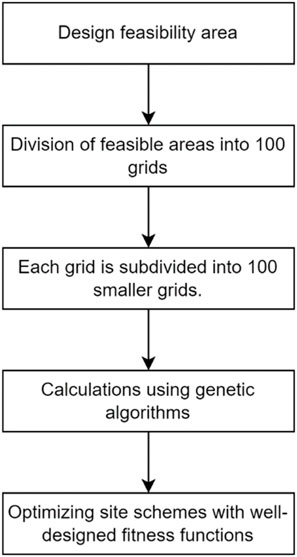
Figure 1. Site selection method.

1. Firstly, a feasible area of $1^{\circ }\times 1^{\circ }$ was designed based on the monitoring target, covering the entire oil field region and representing the theoretically largest feasible area.

2. We divided this feasible area into 100 grids with a spatial resolution of $0.1^{\circ }\times 0.1^{\circ }$. For each grid, we needed to compute the observational efficacy of having a site within that grid, resulting in 100 different footprints. Theoretically, calculating footprints on a denser grid would yield more accurate results, but this would significantly increase computational burden. Moreover, preliminary trials and prior related studies indicated minimal variation in footprints within the $0.1^{\circ }$ range. This influenced our decision to compute footprints on grids with a $0.1^{\circ }$ resolution.

3. Subsequently, we further subdivided the $0.1^{\circ }$ grids into $10\times 10$ fine grids of ${0.01}^{\circ }$ size. We assumed monitoring stations could potentially appear on any of these ${0.01}^{\circ }$ fine grids. Footprints corresponding to each fine grid retained the morphology of the larger grid they belonged to, but we applied a translation to the footprints based on the specific position of the fine grid to ensure accurate alignment with the positions of observation stations.

4. At this stage, we have up to 10,000 feasible candidate positions for observation stations within the entire feasible observation area. Assuming our observation network comprises N stations, we need to select the optimal solution from ${\mathit{C}}_{10000}^{\mathit{n}}$ different possibilities. Exhaustive methods guarantee identifying the best solution but demand computation beyond feasibility. Therefore, this work adopts a genetic algorithm to facilitate the search for the optimal solution. Genetic algorithms excel in navigating complex search spaces efficiently, offering a feasible approach to finding the best solution within a vast set of possibilities. The Genetic Algorithm (GA), originating from bio-inspired computing, is a stochastic global optimization method that simulates biological behavior in nature through computer technology. It is based on Mendel’s laws of genetics, describing natural selection and heredity, simulating phenomena such as replication, crossover, and mutation in this process. This method initially generates an initial population based on specific conditions. Through random selection, crossover, and mutation operations, it evolves the population towards a direction we set by obtaining individuals with higher fitness. Through continuous iterations of evolution, the population of individuals eventually reaches a threshold we define, converging to a group of individuals best adapted to the environment, thus obtaining high-quality solutions to the problem.

5. Formulating the fitness function, a pivotal parameter guiding the iterations of the genetic algorithm, entails its maintenance at a perpetually positive value. This ensures the maximization of the aggregate received emissions at monitoring stations, constituting the fundamental precondition. The initial sub-condition strives to optimize the apportionment of received emissions towards those emanating from emission sources rather than background emissions, while upholding the premise of maximizing the aggregate received emissions. The secondary sub-condition involves normalizing the fitness function within the unit interval [0, 1], serving as a subsequent evaluative criterion. In consideration of these multiple criteria, the fitness function is defined as articulated in Eqs 4, 5.

$\mathit{I}=\mathit{a}\mathit{b}\mathit{s}\left(\mathit{d}\mathit{i}\mathit{f}\mathit{f}\left(\mathbf{tan}\mathit{s}\mathit{i}\mathit{g}\left(\frac{\mathit{\epsilon }}{\mathbf{log}\left(\mathbf{1}+{\mathit{X}}_1*\mathit{H}-\mathbf{log}\left({\mathit{X}}_2*\mathit{H}\right)\right)}\right)\right)\right)(5)$

$=\mathit{a}\mathit{b}\mathit{s}\left(\mathbf{1}-{\left(\mathbf{tan}\mathbf{h}\left(\frac{\mathit{\epsilon }}{\mathbf{log}\left(1+{\mathit{X}}_1*\mathit{H}-\mathbf{log}\left({\mathit{X}}_2*\mathit{H}\right)\right)}\right)\right)}^2)\right.(6)$

In this context, $\mathit{\epsilon }={\mathit{X}}_1*\mathit{H}-{\mathit{X}}_2*\mathit{H},{\mathrm{X}}_1$ (expressed in units of $\mathit{t}\cdot \mathit{h}{\mathit{r}}^{-\mathbf{1}}$) signifies the fraction of emissions originating from the oil and gas sector as stipulated in the GFEI inventory, whereas ${\mathrm{X}}_2$ (expressed in units of $\mathit{t}\cdot \mathit{h}{\mathit{r}}^{-\mathbf{1}}$) denotes the background emissions computed by subtracting the oil and gas-related component from the overall inventory. The term $\mathrm{H}$ (expressed in units of $\mathit{p}\mathit{p}\mathit{b}\mathit{v}\cdot {\left(\mathit{t}\cdot \mathit{h}{\mathit{r}}^{-\mathbf{1}}\right)}^{-\mathbf{1}}$) refers to the footprint. Applying a convolution operation in the spatial domain to both ${\mathrm{X}}_1$ and ${\mathrm{X}}_2$ with the footprint, we derive the natural logarithm of the fitness function’s independent variable by subtracting the convolution of the background difference inventory and footprint from the convolution of the oil and gas inventory with the footprint.

2.3 Emission inventory

The location of methane monitoring stations needs to consider the spatial distribution characteristics of methane emissions, and the current Dongying region has not yet carried out special work on the preparation of methane emission inventories. For this reason, this collected two emission inventories, the Global Fuel Exploitation Inventory (GFEI) and Emissions Database for Global Atmospheric Research (EDGAR), which are commonly used in studies regarding monitoring methane emissions.

The GFEI was developed by Harvard University to assess methane emissions. The inventory has been compared to results from satellites with Global Observations of Atmospheric Methane (GOSAT) and the In-Situ Observation Platform (GLOBALVIEW). The GFEI maps methane emissions from the oil, gas, and coal sectors and subsectors by utilizing national emissions data reported by individual countries to the United Nations Framework Convention on Climate Change (UNFCCC) and mapping them to infrastructure locations to assigned to a $0.1^{\circ }\times 0.1^{\circ }$ grid. Harvard’s updated GFEI v2 provides annual emissions data from 2010 through 2019, including the latest UNFCCC country reports, new oil and gas well locations, and improved spatial distribution of emissions for Canada, Mexico, and China.

EDGAR (Emissions Database for Global Atmospheric Research) is a global emissions database used to estimate emissions of various greenhouse gases and other atmospheric pollutants. The database collects emissions data for individual countries and regions and provides detailed analyses and estimates. The EDGAR database provides emission data for different years, sectors, and countries to help researchers and policymakers understand the trends and distribution of global and regional emissions. For this work, the EDGAR v7.0 was used, the first product of the new EDGAR Community GHG Emissions Database.

3 Results

3.1 Selection of the methane emission inventory

The GFEI emissions inventory focuses solely on the energy industry, primarily divided into two sectors: coal mining and oil development. In the Dongying area, there is almost no methane emissions associated with the coal mining industry. Therefore, the GFEI inventory can directly represent the emissions related to the oil industry in the Dongying area, as shown in Figure 2B.

Figure 2

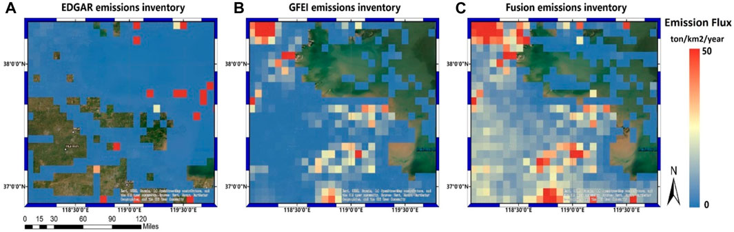
Figure 2. Comparisons of different inventories and fusion of two inventories. (A–C) are EDGAR, GFEI and EDGAR combined with GEFI respectively.

On the other hand, EDGAR covers a wider range of sectors. To ensure comparability between the two inventories, we extract emissions related to the oil and gas sector from the complete EDGAR inventory, as shown in Figure 2A. This extraction process allows for comparison between these two different emissions inventories.

Figure 2 displays that in the Dongying area, a qualitative analysis of the spatial distribution of the two inventories indicates that the GFEI inventory (expressed in units of t∙km^-2∙year⁻²) better reflects the actual spatial distribution of methane emissions in the region. Direct evidence of this is that EDGAR allocates excessive emissions to the offshore area, with the highest value allocated reaching 669.5 t km^-2∙year⁻². This difference may be related to EDGAR using the location of oil and gas extraction facilities as spatial proxies. Offshore drilling platforms may be given greater importance, resulting in excessive emissions being allocated to the offshore area, deviating significantly from the actual situation. Additionally, we also carried out quantitative calculations to analyze the statistical differences between the two inventories. First, compared to the GFEI inventory, the EDGAR inventory (expressed in units of t∙km⁻²∙year⁻²) has a noticeable concentration of emissions allocation. We established a research area with a radius of 50 km centered around oil fields. Within this area, the range of values for the GFEI inventory is 3.86–50.7, while for EDGAR it is 0.17–124.3. Based on this, we separately calculated the means and mean squared errors (MSE) for both inventories, with mean values of 17.42 and 15.39 respectively. Comparing the means, there seems to be no difference between the two. However, when calculating the MSE, we found that the values for GFEI and EDGAR are 101.3 and 1163.4 respectively, indicating that the degree of dispersion in value allocation is much higher in the GFEI inventory than in EDGAR. Referring to the aforementioned EDGAR inventory, which disproportionately allocates contributions from most oil field areas to the offshore area, we believe that under the premise of comparability between the two, the comprehensive spatial distribution and numerical statistical results demonstrate that GFEI is more suitable to represent emissions related to the oil industry in this area.

In addition, in this study, we also collected information about the distribution of local oil field facilities through private communication. However, due to confidentiality agreements in the Chinese oil and gas industry, we are unable to disclose this information in the published work. Through comparison, it was found that the spatial distribution of methane emissions presented by GFEI aligns more closely with the location of local oil and gas extraction and refining facilities. Therefore, in this study, we chose to use the GFEI inventory to describe methane emissions related to the oil and gas industry. At the same time, we use the EDGAR inventory to describe methane emissions from other sectors, separating the EDGAR inventory from the aforementioned reports related to the oil and gas industry, which are the same as the GFEI inventory. The results of the two inventories overlaid can be seen in Figure 2C.

3.2 Footprints under different wind speeds

To calculate the observational effectiveness at specified site locations throughout the year, it’s necessary to compute the annual average footprint for each point. However, conducting extensive simulations using WRF-STILT is practically unfeasible. To derive the annual average footprint for a particular location, we’ve employed a simplified strategy. Initially, we used meteorological reanalysis data to determine the frequency of different wind speeds and directions at a given location.

Subsequently, based on these frequencies, we rotated and weighted precomputed footprints of various levels, ultimately yielding the annual average footprint for that location. This strategy assumes that the shape of the footprint is primarily determined by both wind speed and direction, with geographical location playing a relatively minor role. While this assumption might not hold in areas with complex terrain, Dongying is situated in a plain near the mouth of the Yellow River and lacks significant hills or elevation changes. Given the flat nature of this region, we consider this assumption reasonable.

Therefore, our focus involves calculating typical footprints for each wind speed level per grid, while accounting for wind direction by rotating all precomputed standard footprints to align with an assumed due north wind direction. Wind direction changes can distort footprint shapes, so selecting periods of stable wind conditions becomes crucial to obtain standardized footprints.

In this study, we identified periods corresponding to specific wind speeds based on statistical analyses of wind field data. Subsequently, we selected periods with wind direction stability lasting over 36 h to compute footprints for each wind speed level. Finally, we rotated the computed footprints according to wind direction, with the rotation angle being the angle between the wind direction and true north. Figure 3 displays the situation of standard footprints for various wind speed levels in a 0.1-degree resolution grid, with annotated sampling dates for each wind speed level.

Figure 3

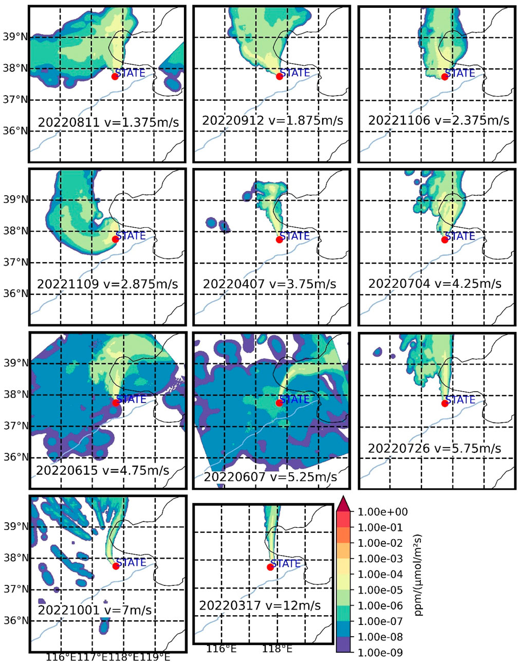
Figure 3. Scenario of footprints at different wind speed levels in a northerly wind direction.

Figure 3 illustrates that as wind speed increases, footprints appear more elongated, and conversely, slower wind speeds result in broader footprints. With higher wind speeds, methane signals captured by observation stations are more concentrated within a narrow area in the upwind direction. Conversely, lower wind speeds make observation stations more susceptible to receiving signals from nearby areas. These characteristics align with the fundamental theory of atmospheric transport, validating the representativeness of footprints computed across different wind speed levels.

It's crucial to note that, for visualization purposes, Figure 3 employs an exponential scale for the intensity of footprints. This implies that even neighboring color gradients represent differences in footprint intensity of over tenfold. During the computation of observational effectiveness, only the strongest color gradient plays a dominant role. The next strongest gradient, when covering a substantial area, might exert some influence, while the remaining gradients have minimal impact on the computed results.

According to Figure 5, the observational effectiveness (emission inventory convolved with footprint, i.e., methane increase) of a site is greater than 150 ppb. It is known from the previous section that the range of GEFI inventory values at the site is from 3.86 to 50.7. As can be seen from Figure 3, when the order of magnitude of the footprint is less than 10⁻⁷, the effect on the observational effectiveness is less than 10⁻² ppb, and we consider that such an effect on the observational effectiveness of the site can be negligible. In Figure 3 the footprint with a wind speed of 1.375 m/s has 85.3% of the data greater than 10⁻⁷, and the footprint with a wind speed of 1.875 m/s has 91.7% of the data greater than 10⁻⁷, these two low wind speed footprints cover a large area and have larger values of footprints, compared to the two very large footprints covering an area with wind speeds of 4.75 m/s and 5.25 m/s, which have 36.4% and 22.8% of the data greater than 10⁻⁷ respectively. We believe that it is easier to receive the impact of emissions from areas other than the oil field area at low wind speeds.

3.3 Annually-averaged footprints

After computing 11 different footprints for each 0.1-degree grid at various wind speed levels, the next step involves further analyzing the wind field characteristics for each grid. Wind rose diagrams serve as standard tools for illustrating the frequency of wind speed and direction in a specific region. In Figure 4, we present the annual wind rose diagram for the coordinates (118.55E, 37.55N). Figure 4A illustrates that southerly winds prevail at this location, often associated with lower wind speeds, while northerly winds tend to bring higher wind speeds.

Figure 4

Figure 4. Wind rose map and annually-averaged footprint map for a given site location. (A–C) are annually-averaged Wind Rose Map at 118.55E,37.55N, annually-averaged footprint case at 118.55E,37.55N, Satellite imagery of the study area respectively.

Utilizing the wind rose diagram allows us to acquire information on the proportion of wind speed and wind direction combinations in a particular area. For instance, if we know that the probability of a wind field with a speed of 3.75 m/s and a direction of WNW is 3%, we would retrieve the standard footprint corresponding to 3.75 m/s wind speed and rotate it counterclockwise by 67.5°. Then, we would multiply this footprint by 0.03. By iterating through all wind speed and wind direction combinations across the grid, we obtain the annual average footprint, as depicted in Figure 4B.

Taking the scenario shown in Figure 4B as an example, we observe that the annual average footprint at this location isn't a uniformly distributed circular shape but rather a complex pattern primarily aligned along the northwest-southeast axis. This indicates that using methods like inverse distance weighting interpolation to generate footprints for observation station locations is unreasonable, as many areas have predominant wind directions, and wind speed and direction aren't uniformly distributed across all directions.

Moreover, it's crucial to emphasize that the simplified strategy employed in this study doesn't account for terrain factors. If, for instance, there are mountains in the southern part of a region, the coverage of different locations towards the south would evidently vary due to their proximity to the mountains. Figure 4C displays satellite imagery of the Dongying vicinity, revealing the eastern part of the North China Plain with only Mount Tai, approximately 200 km southwest of Dongying, amidst vast plains and sea. This issue deserves particular attention for readers seeking a brief overview of this study’s approach. For areas with complex terrain, careful consideration of terrain factors impacting footprints is imperative.

3.4 Site location optimization

Figure 5 illustrates the convergence of the optimization algorithm under different numbers of observation sites (1, 3, 5, 7, 9). The graph indicates that fewer observation sites lead to faster convergence in the optimization process, showing a clear trend: as the number of observation sites decreases, the optimization converges more rapidly, and vice versa.

Figure 5

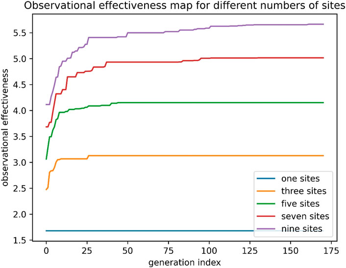
Figure 5. Convergence of optimization processes for different number of sites.

This phenomenon is straightforward to explain: when there’s only one observation site, the optimization program needs to select the best location from 10,000 possible scenarios. However, when the number of sites increases to 3, the feasible solutions drastically expand to C (10, 3) = 1.67 × 10¹¹ possible scenarios. This highlights the challenge in designing observation networks, where the number of feasible solutions escalates rapidly as the number of sites grows—not linearly, but exponentially by orders of 10.

Consequently, the current design of urban observation networks often relies on human judgment and experience, making it difficult to employ quantitative methods for calculation.

In previous studies, researchers employed a random approach to generate a specific number of observation sites and computed the observational effectiveness through multiple iterations. However, this strategy isn't suitable for site selection, which is the problem addressed in this paper.

With just one observation site, the optimization algorithm finds the best solution within 5 iterations. Yet, with 3 observation sites, convergence requires 25 iterations. As the number of sites increases to 5, 7, and 9, the required iterations for convergence further rise to 41, 128, and 162, respectively. These numbers aren't fixed due to the stochastic nature of the GA algorithm—repeated runs may yield varying convergence times—but the overall trend remains consistent.

It's advisable to set an iteration limit for the GA algorithm based on the number of sites, aiding in faster computation results. Generally, as the number of sites increases, a higher maximum iteration count is needed to ensure the algorithm finds the optimal solution.

Our experiments were conducted on a standard personal computer. Optimizing the most complex scenario with 9 sites required approximately 100 min over 200 iterations, a timeframe deemed acceptable for us. However, for larger observation networks or increased grid resolutions, optimization time might significantly increase. At such times, setting a reasonable maximum convergence count becomes a crucial consideration.

Figure 5 demonstrates that as the number of observation sites increases, the overall observational effectiveness improves. However, the degree of improvement diminishes with a rising number of observation sites. The observational effectiveness achieved by the optimal solutions with 1, 3, 5, 7, and 9 sites are 1.7, 3.1, 4.2, 5, and 5.6, respectively.

It's expected that with further increases in the number of observation sites, the enhancement in observational effectiveness will continue to decrease, possibly reaching a maximum value. The construction cost of the observation network grows linearly with the number of observation sites. Therefore, it's essential to determine a balance point that achieves a compromise between cost and observational capability.

3.5 Optimized solution for monitoring networks of different sites

Figure 6, Figure 7, and Figure 8 respectively display the positions of five, seven, and nine optimized stations generated by the optimization algorithm, along with the annual average footprints (We only show the fraction greater than 1 ppbv∙(t∙hr-1), since the previously mentioned fraction less than this value is negligible for the observational power of the site) at each station based on GFEI emission inventory. The background is a satellite image of the Dongying oil field. Among them, different colored squares represent different methane concentrations in the GEFI inventory, the darker the color the higher the methane concentration. The green origin represents the optimized site location. The irregular cloudy portion represents the annual average methane backward footprint of the site. We utilize the GFEI inventory to represent methane concentration in the area, combined with the annual average footprints to assess the observational capabilities at each station. It's evident that the stations are primarily located in areas with higher methane concentrations (>10 t km^-2∙year⁻²) according to the GFEI inventory. The alignment between the annual average footprints and the GFEI inventory is relatively comprehensive, particularly concentrated in the southern part of Dongying (Shengli Oilfield). As the number of stations increases, the distribution becomes more stable. The addition of stations from five to nine doesn't alter the general positions of the existing stations but rather includes stations in areas with higher methane concentrations according to the GFEI inventory, with more stations distributing in the southern part of Dongying. Because emissions are more concentrated and intense in the southern part of Dongying, which is the main location for the placement of oil field facilities, it makes perfect sense to place more sites there.

Figure 6

Figure 6. Optimum solution for 5 sites.

Figure 7

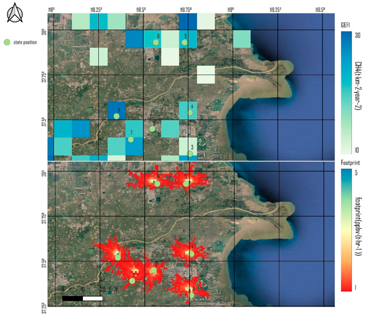
Figure 7. Optimum solution for 7 sites.

Figure 8

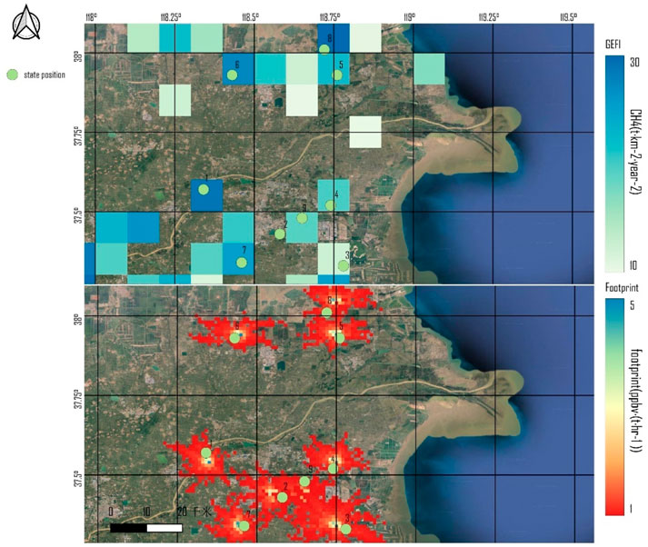
Figure 8. Optimum solution for 9 sites.

As depicted in Figure 5, the increase in observational effectiveness gradually diminishes with a rise in the number of stations, the number of stations increased from 5 to 7 to 9, and the observational effectiveness increased from 3.1 to 4.2 to 5. In Figure 6, the stations are mainly situated in regions with darker colors in the GFEI inventory, while with an increase in station numbers, the locations of the stations correspond to lighter colors, indicating lower methane concentrations in those areas. Consequently, the original stations are presumed to have higher observational capabilities compared to the newly added stations. This could be attributed to the overlapping observation ranges between the new and original stations, where the methane concentration at the new station locations is lower than that of the original stations. Figure 7 adds Site 6 (118.57E, 37.93N), Site 7 (118.55E, 37.45N), and an increase in observational effectiveness of 1.1 compared to Figure 6. Site 6 has a 3.4 percent average annual footprint coverage (How much the footprints overlap) with the original site, and Site 7 has a 31.2 percent average annual footprint coverage with the original site. Figure 8 adds Site 8 (118.72E, 38.01N), Site 9 (118.65E, 37.48N), and an increase in observational effectiveness of 0.8 compared to Figure 7. Site 8 has 2.1 percent annual average footprint coverage with the original site, and Site 9 has 67.5 percent annual average footprint coverage with the original site. The above results are consistent with a decreased increase in observational effectiveness due to the overlap of site observation ranges.

Considering the coverage range of station observations and the actual deployment costs, we can roughly determine the required number and positions of stations. Under the premise of guaranteeing the basic observation range, the selection of more stations with better observation effectiveness is an urgent problem to be solved. The change in observational effectiveness from seven to nine stations is not a significant improvement, so seven stations can be considered the basic placement standard when considering costs, and a number of stations lower than seven may result in an incomplete range of observations, which can be increased if the budget is sufficient.

The optimized station locations correspond well with reality, mostly positioned in areas with higher methane concentrations according to the GFEI inventory. Additionally, with an increase in optimized station quantity, the station distribution becomes more stable.

4 Discussion

Given the extensive dispersion of oil field infrastructure throughout the entire region rather than concentrated layouts, the feasible range for monitoring points is considerably broad. This necessitates narrowing down the feasible range of monitoring points before numerical optimization due to the high spatiotemporal complexity, which could lead to optimization difficulties and potential non-convergence. The wind field data used in this study originated from hourly 10 m wind field data from ERA-5 reanalysis. However, due to the 0.25°×0.25° grid accuracy of ERA-5 reanalysis data, which cannot match the precision of the footprints, interpolation methods were applied to adapt the wind field data to a 0.1°×0.1° grid. Kriging interpolation was utilized for this study, and it's essential to note that the precision of the 0.1° wind field vector speed might be influenced by the interpolation method chosen.

Regarding the generation of annual average footprints, we divided it into 12 wind field levels based on wind speed and frequency. Footprints were rotated under each of the 12 wind levels and eventually combined to form the annual average footprint. To adapt each footprint level’s wind speed selection, we attempted to select 12 wind field intervals with approximately the same frequency. The wind speed was set at the midpoint of each frequency interval. However, finding periods with stable wind speeds and directions, especially in summer, particularly for wind speeds below 6 m/s, was challenging. Considering that approximately 80% of the wind field in the oil field region is concentrated below 6 m/s, evaluating the stability of the wind field data, particularly at 10m, becomes crucial.

The emission inventory utilized in this study is a combination of GFEI and EDGAR data. GFEI mainly represents the energy industry, while EDGAR provides more comprehensive coverage. The site selection process focuses on maximizing the observational benefits while ensuring maximum oil and gas content in the observed emissions. As per the comparison between the GFEI and EDGAR inventories, the former is selected for oil and gas emissions, while the latter represents the background emissions after subtracting oil and gas emissions. Errors in both inventories accumulate spatially and sectorally following the law of error propagation. Both inventories have a spatial resolution of 0.1°×0.1°, which needs to be adapted to 0.01°×0.01° to match the footprints’ resolution. Unlike the wind field reanalysis data, the emission inventory does not exhibit spatial correlation; hence, resampling was used during the interpolation, causing limitations in the accuracy of emission fluxes at each 0.01° grid point.

Increasing the number of stations leads to a linear increase in computational burden, which is also influenced by factors like algorithm iteration counts, study area size, and the spatial resolution of the emission inventory and footprints. The maximum station count in this experiment was nine, taking approximately 10 min. For instance, increasing the station count to 90 or 900 would lead to computation times of 100 min or 1000 min, respectively. However, this computational burden is manageable within realistic scenarios, considering the upper limit of 9600 for the station locations, where linear computational increments occur for station counts below this limit. Realistically, under limited funding, the actual station count is unlikely to reach this upper limit, thus making the increased computational burden acceptable.

Expanding the diffusion range of footprints, enlarging the study area, or enhancing the spatial resolution of emission inventories and footprints on the existing experimental basis will result in a multiple-fold increase in computational burden. Due to practical research considerations and budget constraints, such a high computational burden might not be feasible. Hence, considering these factors, planning a station optimization strategy with an acceptable computational burden is entirely plausible.

At present, only in situ measurement equipment will be deployed at each site. However, there are plans to supplement this with Differential Absorption LiDAR (Shi et al., 2021; Zhang H. et al., 2023) in the future. This technology is capable of measuring range-resolved atmospheric CH4 concentrations (Han et al., 2017; Shi et al., 2020), thereby extending coverage over a larger area. Besides, The main oil production area of the Shengli Oilfield is located near the mouth of the Yellow River. Distance-resolved observational data helps distinguish methane emissions from natural ecosystems and anthropogenic processes (Qiu et al., 2023).

5 Conclusion

This study employed multisource remote sensing and geographic data to conduct an initial screening of methane emission areas. Meteorological reanalysis data was used to drive a high-resolution atmospheric transport model, which calculated the footprints of specified observation points. A Monte Carlo method was utilized to randomly generate a designated number of observation points. The Boltzmann-GA optimization model was then employed to iteratively adjust the positions of these observation points until fitness convergence was achieved. By integrating atmospheric transport modeling, Boltzmann-GA optimization algorithm, and remote sensing environmental monitoring data, this study successfully designed and optimized a methane monitoring network for oil fields, providing technical support for methane emission monitoring in the energy industry.

In the current scenario where reference examples and guidelines for designing methane monitoring networks are lacking, the findings of this study fill the gap and have the potential to become an industry standard for effective site selection in methane monitoring in oil fields. The designed monitoring network, which leverages multiple data sources and advanced optimization algorithms, exhibits high accuracy and coverage in methane emission monitoring. Furthermore, the proposed methodology is applicable to methane monitoring and environmental surveillance tasks in other regions.

In conclusion, this study provides an effective approach for designing and optimizing methane monitoring networks in oil fields. Future research can further enhance and expand upon this methodology to cater to monitoring requirements in different regions and application scenarios. By continuously improving monitoring technologies and methodologies, we will be better equipped to manage and control methane emissions in the energy industry, thereby achieving sustainable energy development and environmental protection goals.

Data availability statement

The raw data supporting the conclusion of this article will be made available by the authors, without undue reservation.

Author contributions

LF: Writing–original draft, Writing–review and editing, Conceptualization, Data curation, Formal Analysis, Funding acquisition, Investigation, Methodology, Project administration, Resources, Software, Supervision, Validation, Visualization. XH: Data curation, Formal Analysis, Writing–original draft, Writing–review and editing. XW: Project administration, Resources, Software, Writing–original draft. KM: Methodology, Validation, Visualization, Writing–review and editing. XZ: Conceptualization, Data curation, Formal Analysis, Writing–review and editing. YY: Investigation, Methodology, Project administration, Writing–original draft. FR: Methodology, Project administration, Software, Visualization, Writing–original draft. HS: Funding acquisition, Investigation, Methodology, Project administration, Writing–original draft. JY: Data curation, Investigation, Methodology, Resources, Software, Validation, Visualization, Writing–original draft, Writing–review and editing.

Funding

The author(s) declare that financial support was received for the research, authorship, and/or publication of this article. This study was funded by Hubei Provincial Natural Science Foundation (Grant Nos 2023AFB834 and 202CFD015), National Natural Science Foundation of China (Grant No. 4197283) and the Fundamental Research Funds for the Central Universities (2042023kf1050). The numerical calculations in this paper have been done on the supercomputing system in the Supercomputing Center of Wuhan University.

Conflict of interest

Authors LF, XH, XW, KM, XZ, YY, FR, and HS were employed by the Ltd. Of Sinopec Shengli OilField.

The remaining author declares that the research was conducted in the absence of any commercial or financial relationships that could be construed as a potential conflict of interest.

Publisher’s note

All claims expressed in this article are solely those of the authors and do not necessarily represent those of their affiliated organizations, or those of the publisher, the editors and the reviewers. Any product that may be evaluated in this article, or claim that may be made by its manufacturer, is not guaranteed or endorsed by the publisher.

References

Chen, Y. L., Sherwin, E. D., Berman, E. S., Jones, B. B., Gordon, M. P., Wetherley, E. B., et al. (2022). Quantifying regional methane emissions in the New Mexico Permian Basin with a comprehensive aerial survey. Environ. Sci. Technol. 56 (7), 4317–4323. doi:10.1021/acs.est.1c06458

PubMed Abstract | CrossRef Full Text | Google Scholar

Erland, B. M., Thorpe, A. K., and Gamon, J. A. (2022). Recent advances toward transparent methane emissions monitoring: a review. Environ. Sci. Technol. 56 (23), 16567–16581. doi:10.1021/acs.est.2c02136

PubMed Abstract | CrossRef Full Text | Google Scholar

Gong, S., and Shi, Y. (2021). Evaluation of comprehensive monthly-gridded methane emissions from natural and anthropogenic sources in China. Sci. Total Environ. 784, 147116. doi:10.1016/j.scitotenv.2021.147116

PubMed Abstract | CrossRef Full Text | Google Scholar

Han, G., Cui, X., Liang, A., Ma, X., Zhang, T., and Gong, W. (2017). A CO2 profile retrieving method based on Chebyshev fitting for ground-based DIAL. IEEE Trans. Geoscience Remote Sens. 55 (99), 6099–6110. doi:10.1109/tgrs.2017.2720618

CrossRef Full Text | Google Scholar

Han, G., Xin, M., Gong, W., Chen, W., and Liu, J. (2021). Quantifying CO2 uptakes over oceans using lidar: a tentative experiment in bohai bay. Geophys. Res. Lett. 48 (9). doi:10.1029/2020gl091160

CrossRef Full Text | Google Scholar

He, W., van der Velde, I. R., Andrews, A. E., Sweeney, C., Miller, J., Tans, P., et al. (2018). CTDAS-Lagrange v1.0: a high-resolution data assimilation system for regional carbon dioxide observations. Geosci. Model Dev. 11 (8), 3515–3536. doi:10.5194/gmd-11-3515-2018

CrossRef Full Text | Google Scholar

Hu, H., Landgraf, J., Detmers, R., Borsdorff, T., Aan de Brugh, J., Aben, I., et al. (2018). Toward global mapping of methane with TROPOMI: first results and intersatellite comparison to GOSAT. Geophys. Res. Lett. 45 (8), 3682–3689. doi:10.1002/2018gl077259

CrossRef Full Text | Google Scholar

Irakulis-Loitxate, I., Guanter, L., Liu, Y. N., Varon, D. J., Maasakkers, J. D., Zhang, Y., et al. (2021). Satellite-based survey of extreme methane emissions in the Permian basin. Sci. Adv. 7 (27), eabf4507. doi:10.1126/sciadv.abf4507

PubMed Abstract | CrossRef Full Text | Google Scholar

Jacob, D. J., Turner, A. J., Maasakkers, J. D., Sheng, J., Sun, K., Liu, X., et al. (2016). Satellite observations of atmospheric methane and their value for quantifying methane emissions. Atmos. Chem. Phys. 16 (22), 14371–14396. doi:10.5194/acp-16-14371-2016

CrossRef Full Text | Google Scholar

Jacob, D. J., Varon, D. J., Cusworth, D. H., Dennison, P. E., Frankenberg, C., Gautam, R., et al. (2022). Quantifying methane emissions from the global scale down to point sources using satellite observations of atmospheric methane. Atmos. Chem. Phys. 22 (14), 9617–9646. doi:10.5194/acp-22-9617-2022

CrossRef Full Text | Google Scholar

Kang, M., Christian, S., Celia, M. A., Mauzerall, D. L., Bill, M., Miller, A. R., et al. (2016). Identification and characterization of high methane-emitting abandoned oil and gas wells. Proc. Natl. Acad. Sci. 113 (48), 13636–13641. doi:10.1073/pnas.1605913113

PubMed Abstract | CrossRef Full Text | Google Scholar

Kirschke, S., Bousquet, P., Ciais, P., Saunois, M., Canadell, J. G., Dlugokencky, E. J., et al. (2013). Three decades of global methane sources and sinks. Nat. Geosci. 6 (10), 813–823. doi:10.1038/ngeo1955

CrossRef Full Text | Google Scholar

Laughner, J. L., Toon, G. C., Mendonca, J., Petri, C., Roche, S., Wunch, D., et al. (2023). The total carbon column observing network's GGG2020 data version. Earth Syst. Sci. Data Discuss. 2023, 1–86. doi:10.5194/essd-2023-331

CrossRef Full Text | Google Scholar

Lin, J. C., Gerbig, C., Wofsy, S. C., Andrews, A. E., Daube, B. C., Davis, K. J., et al. (2003). A near-field tool for simulating the upstream influence of atmospheric observations: the Stochastic Time-Inverted Lagrangian Transport (STILT) model. J. Of Geophys. Research-Atmospheres 108 (D16). doi:10.1029/2002jd003161

CrossRef Full Text | Google Scholar

Liu, B., Ma, X., Guo, J., Wen, R., Li, H., Jin, S., et al. (2024). Extending the wind profile beyond the surface layer by combining physical and machine learning approaches. Atmos. Chem. Phys. 24 (7), 4047–4063. doi:10.5194/acp-24-4047-2024

CrossRef Full Text | Google Scholar

Omara, M., Gautam, R., O'Brien, M. A., Himmelberger, A., Franco, A., Meisenhelder, K., et al. (2023). Developing a spatially explicit global oil and gas infrastructure database for characterizing methane emission sources at high resolution. Earth Syst. Sci. Data Discuss. 15, 3761–3790. doi:10.5194/essd-15-3761-2023

CrossRef Full Text | Google Scholar

Pei, Z., Han, G., Mao, H., Chen, C., Shi, T., Yang, K., et al. (2023a). Improving quantification of methane point source emissions from imaging spectroscopy. Remote Sens. Environ. 295, 113652. doi:10.1016/j.rse.2023.113652

CrossRef Full Text | Google Scholar

Pei, Z., Han, G., Shi, T., Ma, X., and Gong, W. (2023b). A XCO retrieval algorithm coupled spatial correlation for the aerosol and carbon detection lidar. Atmos. Environ. 309, 119933. doi:10.1016/j.atmosenv.2023.119933

CrossRef Full Text | Google Scholar

Pei, Z. P., Han, G., Ma, X., Su, H., and Gong, W. (2020). Response of major air pollutants to COVID-19 lockdowns in China. Sci. Total Environ. 743, 140879. doi:10.1016/j.scitotenv.2020.140879

PubMed Abstract | CrossRef Full Text | Google Scholar

Pei, Z. P., Han, G., Ma, X., Shi, T., and Gong, W. (2022). A method for estimating the background column concentration of CO2 using the Lagrangian approach. Ieee Trans. Geoscience And Remote Sens. 60, 1–12. doi:10.1109/tgrs.2022.3176134

CrossRef Full Text | Google Scholar

Peng, S., Lin, X., Thompson, R. L., Xi, Y., Liu, G., Hauglustaine, D., et al. (2022). Wetland emission and atmospheric sink changes explain methane growth in 2020. Nature 612 (7940), 477–482. doi:10.1038/s41586-022-05447-w

PubMed Abstract | CrossRef Full Text | Google Scholar

Pillai, D., Gerbig, C., Kretschmer, R., Beck, V., Karstens, U., Neininger, B., et al. (2012). Comparing Lagrangian and Eulerian models for CO2 transport - a step towards Bayesian inverse modeling using WRF/STILT-VPRM. Atmos. Chem. And Phys. 12 (19), 8979–8991. doi:10.5194/acp-12-8979-2012

CrossRef Full Text | Google Scholar

Qiu, R., Han, G., Li, S., Tian, F., Ma, X., and Gong, W. (2023). Soil moisture dominates the variation of gross primary productivity during hot drought in drylands. Sci. Total Environ. 899, 165686. doi:10.1016/j.scitotenv.2023.165686

PubMed Abstract | CrossRef Full Text | Google Scholar

Qiu, R., Han, G., Li, X., Xiao, J., Liu, J., Wang, S., et al. (2024). Contrasting responses of relationship between solar-induced fluorescence and gross primary production to drought across aridity gradients. Remote Sens. Environ. 302, 113984. doi:10.1016/j.rse.2023.113984

CrossRef Full Text | Google Scholar

Schissel, C., and Allen, D. T. (2022). Impact of the high-emission event duration and sampling frequency on the uncertainty in emission estimates. Environ. Sci. Technol. Lett. 9, 1063–1067. doi:10.1021/acs.estlett.2c00731

CrossRef Full Text | Google Scholar

Shi, T., Han, G., Ma, X., Mao, H., Chen, C., Han, Z., et al. (2023a). Quantifying factory-scale CO2/CH4 emission based on mobile measurements and EMISSION-PARTITION model: cases in China. Environ. Res. Lett. 18 (3), 034028. doi:10.1088/1748-9326/acbce7

CrossRef Full Text | Google Scholar

Shi, T., Han, G., Ma, X., Pei, Z., Chen, W., Liu, J., et al. (2023b). Quantifying strong point sources emissions of CO2 using spaceborne LiDAR: method development and potential analysis. Energy Convers. Manag. 292, 117346. doi:10.1016/j.enconman.2023.117346

CrossRef Full Text | Google Scholar

Shi, T., Han, G., Ma, X., Zhang, M., Pei, Z., Xu, H., et al. (2020). An inversion method for estimating strong point carbon dioxide emissions using a differential absorption Lidar. J. Clean. Prod. 271, 122434. doi:10.1016/j.jclepro.2020.122434

CrossRef Full Text | Google Scholar

Shi, T., Han, Z., Han, G., Ma, X., Chen, H., Andersen, T., et al. (2022). Retrieving CH 4-emission rates from coal mine ventilation shafts using UAV-based AirCore observations and the genetic algorithm–interior point penalty function (GA-IPPF) model. Atmos. Chem. Phys. 22 (20), 13881–13896. doi:10.5194/acp-22-13881-2022

CrossRef Full Text | Google Scholar

Sun, Y., Yin, H., Wang, W., Shan, C., Notholt, J., Palm, M., et al. (2022). Monitoring greenhouse gases (GHGs) in China: status and perspective. Atmos. Meas. Tech. 15 (16), 4819–4834. doi:10.5194/amt-15-4819-2022

CrossRef Full Text | Google Scholar

Thompson, R. L., and Stohl, A. (2014). FLEXINVERT: an atmospheric Bayesian inversion framework for determining surface fluxes of trace species using an optimized grid. Geosci. Model Dev. 7 (5), 2223–2242. doi:10.5194/gmd-7-2223-2014

CrossRef Full Text | Google Scholar

Tu, Q., Hase, F., Schneider, M., García, O., Blumenstock, T., Borsdorff, T., et al. (2022). Quantification of CH<sub>4</sub> emissions from waste disposal sites near the city of Madrid using ground- and space-based observations of COCCON, TROPOMI and IASI. Atmos. Chem. Phys. 22 (1), 295–317. doi:10.5194/acp-22-295-2022

CrossRef Full Text | Google Scholar

Turner, A. J., Shusterman, A. A., McDonald, B. C., Teige, V., Harley, R. A., and Cohen, R. C. (2016). Network design for quantifying urban CO2 emissions: assessing trade-offs between precision and network density. Atmos. Chem. And Phys. 16 (21), 13465–13475. doi:10.5194/acp-16-13465-2016

CrossRef Full Text | Google Scholar

Varon, D. J., Jacob, D. J., McKeever, J., Jervis, D., Durak, B. O. A., Xia, Y., et al. (2018). Quantifying methane point sources from fine-scale satellite observations of atmospheric methane plumes. Atmos. Meas. Tech. 11 (10), 5673–5686. doi:10.5194/amt-11-5673-2018

CrossRef Full Text | Google Scholar

Varon, D. J., McKeever, J., Jervis, D., Maasakkers, J. D., Pandey, S., Houweling, S., et al. (2019). Satellite discovery of anomalously large methane point sources from oil/gas production. Geophys. Res. Lett. 46, 13507–13516. doi:10.1029/2019gl083798

CrossRef Full Text | Google Scholar

Wu, D., Lin, J. C., Fasoli, B., Oda, T., Ye, X., Lauvaux, T., et al. (2018). A Lagrangian approach towards extracting signals of urban CO<sub>2</sub> emissions from satellite observations of atmospheric column CO<sub>2</sub> (XCO<sub>2</sub>): X-Stochastic Time-Inverted Lagrangian Transport model (“X-STILT v1”). Geosci. Model Dev. 11 (12), 4843–4871. doi:10.5194/gmd-11-4843-2018

CrossRef Full Text | Google Scholar

Wu, D., Yue, Y., Jing, J., Liang, M., Sun, W., Han, G., et al. (2023). Background characteristics and influence analysis of greenhouse gases at jinsha atmospheric background station in China. Atmosphere 14 (10), 1541. doi:10.3390/atmos14101541

CrossRef Full Text | Google Scholar

Yang, J., Gan, R., Luo, B., Wang, A., Shi, S., and Du, L. (2024). An improved method for individual tree segmentation in complex urban scenes based on using multispectral LiDAR by deep learning. IEEE J. Sel. Top. Appl. Earth Observations Remote Sens. 17, 6561–6576. doi:10.1109/jstars.2024.3373395

CrossRef Full Text | Google Scholar

Ye, X., Lauvaux, T., Kort, E. A., Oda, T., Feng, S., Lin, J. C., et al. (2020). Constraining fossil Fuel CO2 emissions from urban area using OCO-2 observations of total column CO2. J. Geophys. Res. Atmos. 125 (8), e2019JD030528. doi:10.1029/2019jd030528

CrossRef Full Text | Google Scholar

Zhang, H., Ma, X., Chen, W., Zhang, X., and Liu, J. (2023b). Robust algorithm for precise X CO2 retrieval using single observation of IPDA LIDAR. Opt. Express 31 (7), 11846–11863. doi:10.1364/oe.482629

PubMed Abstract | CrossRef Full Text | Google Scholar

Zhang, J., Mao, H., Pei, Z., Ma, X., and Jia, W. (2022). The spatial and temporal distribution patterns of XCH4 in China: new observations from TROPOMI. Atmosphere 13 (2), 177. doi:10.3390/atmos13020177

CrossRef Full Text | Google Scholar

Zhang, Y., Gautam, R., Pandey, S., Omara, M., Maasakkers, J. D., Sadavarte, P., et al. (2020). Quantifying methane emissions from the largest oil-producing basin in the United States from space. Sci. Adv. 6 (17), eaaz5120. doi:10.1126/sciadv.aaz5120

PubMed Abstract | CrossRef Full Text | Google Scholar

Zhang, Y., Wang, W., He, J., Jin, Z., and Wang, N. (2023a). Spatially continuous mapping of hourly ground ozone levels assisted by Himawari-8 short wave radiation products. GIScience Remote Sens. 60 (1), 2174280. doi:10.1080/15481603.2023.2174280

CrossRef Full Text | Google Scholar