 Zhuo Chen
 Tao Liu1,3*
94% of researchers rate our articles as excellent or good
Learn more about the work of our research integrity team to safeguard the quality of each article we publish.
Find out more
ORIGINAL RESEARCH article
Front. Environ. Sci., 10 July 2024
Sec. Environmental Informatics and Remote Sensing
Volume 12 - 2024 | https://doi.org/10.3389/fenvs.2024.1393031
This article is part of the Research TopicRemote Sensing in Ecological Environments: Innovations and AchievementsView all 8 articles
The climate change and extension of human activities are shedding more stresses on ecosystems. Ecological zoning could help manage the ecosystem and deal with environmental problems more effectively. Geology and topography could affect the ecology primarily and are vital perspectives on ecological zoning. It is worth preliminarily understanding the spatial-temporal patterns of ecological-environmental attributes within various geological-topographical ecological zones (GTEZs). The objective of this study was to delineate GTEZs and present a spatial-temporal analysis on soil and land surface parameters within GTEZs. Firstly, Landsat imageries, high resolution satellite imagery products, digital elevation model, regional geological map, black soil thickness, soil bulk density, meteorological data, and ground survey were collected and conducted. Secondly, GTEZs in Hailun District were delineated according to geological and topographical background. Thirdly, soil composition, and monthly land surface temperature (LST), enhanced vegetation index (EVI), net primary productivity (NPP) were derived from ground survey and Landsat imageries. Finally, spatial-temporal patterns of various ecological-environmental attributes within different GTEZs were preliminarily revealed and analyzed. Results show that sand alluvial plain zone and silt-clay undulating plain zone mainly possess thick soil with fine-medium granule and higher bulk density, and are mainly covered by crops and grass, vegetation flourish the most in August with the highest monthly EVI and NPP. While the sand-conglomerate hill zone, sandstone hill zone, and granite hill zone possess relatively thin soil with medium-coarse granule and lower bulk density, and are mainly covered by forest, vegetation flourish the most in June and July, and has the highest yearly total NPP. With thinner soil thickness and higher NPP, hill zones tend to have more vulnerability to disturbance and more contribution to carbon neutrality target.
Climate change is an inevitable theme faced by the current era (NAS, 2020). Besides, anthropogenic factors such as expansions of human activity range, industrialization, and environmental policies also have a significant impact on ecosystems (Liu et al., 2018; Wang et al., 2018). To better plan and manage natural resources, researchers have innovatively assessed the contributions of climate change and anthropogenic factors in some respects and regions (Shahid et al., 2018). Ecological zoning may also better help preserve, manage, utilize the ecosystem (Klimina and Ostroukhov, 2021; Suska et al., 2023) and deal with environmental problems like climate change, pollution, biodiversity loss, and irrational construction expansion (Gao et al., 2019; Deng and Cao, 2023). Ecological zone or region could be defined as land or water that contain distinct assemblages of natural communities, these communities share a large majority of their species, dynamics, environmental, geographic, geological, climatic conditions and function together effectively with internal consistency (Nilsson, 2002; Thompson et al., 2004). Different ecological zones could response distinctly to climate change and human activities (Bracewell et al., 2021; Chen et al., 2024).
Various methods have been applied to ecological zoning, including machine learning (ML), spatial modeling, and GIS-based analysis. ML method uses zone samples and attribute layers to train the ML model, and then identify target zone in other locations (Li Z. et al., 2023), it could demonstrate superhuman performance in many tasks, but may fail in model simplicity and interpretability (Linardatos et al., 2021). Unlike the iteration conducted in ML method, spatial modeling relies more on theoretical reasoning and traditional mathematical algorithms, it combines target-related attributes using certain formulas (Xu et al., 2024), the attribute layers applied in ML and spatial modeling are quantitative data with digital value or codes (Amin et al., 2022; Li Z. et al., 2023). The concept of GIS-based analysis is broad, including quantitative calculation and qualitative visual delineation (Wang et al., 2019; Jafar et al., 2020), which makes this method flexible and adaptive, but sometimes may lead to subjective. A number of ecological zoning has been conducted on various scales with diverse purposes and emphases. Ministry of Environmental Protection of Chinese government and Chinese Academy of Sciences (MEP and CAS, 2015) delineated approximately 242 ecological functional zones in China. Liu et al. (2021) emphasized the effects of soil erosion, mining, precipitation, vegetation changing, cultivated land grade, and incomes of people, then assessed various watersheds and obtained ecological zones in the Qilian Mountain Area, China. Xiao et al. (2022) emphasized the optimization of land space development patterns, then calculated the change trend of “production-living-ecology” spatial conflict, and eventually obtained ecological zones in Qianjiang City, China. Li H. et al (2023) emphasized the ecological functions and services, took both natural conditions and socioeconomics into consideration, and classified ecological functional zones in Qinghai-Tibet Plateau, China. Staselko et al. (2020) emphasized the significance of lichens as indicators of environmental status, and divided Elista City, Russia into three zones according to the distribution of lichen groups. Wen et al. (2021) emphasized aquifer structures, cycle process, and spatial variation of ground water systems, and divided the groundwater in Asia into eleven primary systems according to geological structures, climate, landforms, and hydrogeological structures. Bian et al. (2023) emphasized the landscape ecological risk, and graded the landscape ecological risk of counties in China from 2000 to 2015. Jiang et al. (2022) emphasized the importance of ecological network to biodiversity, and carried out ecological zoning on the basis of ecological source area ratio, ecological source connectivity, ecological corridor area ratio, ecological corridor current, pinch-point area ratio, and barrier area ratio in Yunnan Province, China.
In addition to topography, land use, water, habitat connectivity, function, and ecological risk, geology could also be a vital perspective on ecological zoning. Researchers have recognized the influence of geological factors to an ecosystem early. A concept of “ecological geology system” was introduced in 1997 and defined as a certain volume of the lithosphere with biota, including humans and the social function in it (Trofimov, 2009). Concept of “earth’s critical zones” was also introduced in 2001 to investigate rock, soil, water, air, and living organisms as a whole (Nie et al., 2020). Unlike the other conditions, the characteristics of geology and topography are relatively stable, and could affect the spatiotemporal pattern of ecology at regional scale (Tao et al., 2022). Tao et al. (2022) calculated the coupling coordination degrees (CCDs) of geology-topography and ecology in different ecological regions in Northeastern China, and results showed that the CCDs were distinct in the Songnen Plain and Lesser Khingan Range, China. Chakraborty (2018) studied the synthetic effects of geology, topography, chemical elements, and humans on ground landscapes. Hou and Gao (2020) studied the spatial relationships between karst landscape pattern and vegetation activities in Guizhou Province, China, results showed that negative effects on vegetation activity from landscape structural changes were more significant in the carbonate areas, which might be due to the more vulnerable ecosystems there. Chen et al. (2022) took soil thickness, soil nitrogen content, and slope into consideration during the ecological-environment assessment in the Northeastern China. Flores et al. (2019) studied the relationships between landform and vegetation in the Cerro Zonda Mountain, Argentina, and found that slope and roughness would determine the vegetation coverage at regional scale, and high coverage of rock fragments would determine the vegetation richness and diversity at local scale. Guo et al. (2023) studied the geological genesis of some typical land desertification, salinization, and rocky desertification areas in China from the perspective of parent materials/rocks weathering process, and established models to help understand the genesis of these eco-geological problems.
Soil is the foundation of vegetation and agricultural activities, and affects the local ecological vulnerability. Many subsurface processes in different landscapes are primarily dominated by soil thickness (Catani et al., 2010), plant roots cannot develop vertically on hills with shallow soil thickness (Chen et al., 2022). Black soil is rich in organic carbon with superior physical and chemical characteristics (Fang, 2021), thicker black soil provides better nutrient conditions. Different soil granularity could result in various moisture (Sabathier et al., 2021), soil bulk density is an indicator for soil compaction and porosity (Suuster et al., 2011), and could affect the water holding capacity, infiltration, aeration, root growth, and carbon stocks (Zhao et al., 2021). Apart from soil parameters, land surface temperature (LST), normalized difference vegetation index (NDVI) are parameters widely used to assess ecological conditions (Firozjaei et al., 2020; Qureshi et al., 2020). LST is determined by local surface conditions and macro-atmospheric conditions (Liang et al., 2019), and is a key parameter for monitoring and evaluating the surface physical, chemical, and biological processes (Alavi Panah et al., 2017). Vegetation is vital to climate regulation, geochemical cycling, water flux between soil and atmosphere, and soil-water conservation (Bai et al., 2024), so NDVI is widely used in the study of plant physical characteristics and ecology (Myneni and Williams, 1994; Chen et al., 2023). However, NDVI would face with the saturation problem when leaf area index exceeds 4, thus affecting the accurate estimation of vegetation conditions (Huete et al., 2002; Xu et al., 2020). Compared with NDVI, the enhanced vegetation index (EVI) is more sensitive to dense vegetation and variation in the viewing geometry, surface albedo, and Sun elevation angle across variable terrain, making EVI robust for vegetation biomass and quality estimation (Garroutte et al., 2016). The combined influence of climate change and human activities calls for carbon neutrality (Lyu et al., 2023), net primary productivity (NPP) could directly reflect the production capacity of the vegetation and play as the reference of carbon exchanges (Cloern et al., 2021). Human activities have reduced global NPP available to terrestrial ecosystems by approximately 25% (Haberl et al., 2007), so beyond LST and EVI, it is also worth preliminarily understanding the NPP patterns within various ecological zones.
Seasonality is the regular and periodic changes of a condition on an annual timescale (Williams et al., 2017), and can essentially influence an ecosystem yearly (Hastings, 2014) and alter the phenology of species in important ways, but seasons were constantly ignored in the investigations of ecological system and process (White and Hastings, 2020). At present, researchers mainly focused on the spatial or yearly conditions of hydrogeology, landform, precipitation, soil erosion, vegetation, landscape risk, land space development, cultivation, ecological service, ecological network, biodiversity, floras, and economic development within or between ecological zones (Staselko et al., 2020; Liu et al., 2021; Wen et al., 2021; Jiang et al., 2022; Xiao et al., 2022; Li H. et al., 2023; Bian et al., 2023), few studies delineated ecological zones from the geological-topographical perspective, nor considered the diversities of soil and spatial-temporal patterns of temperature, vegetation, and carbon fixation effects as season changes in different geological-topographical ecological zones (GTEZs). Research on this recommended theme is helpful to understanding the seasonal influence on ecological-environmental cyclic change, and could also furtherly provide information for the seasonal surface energy budget and carbon balance research (Dang et al., 2020; Lian et al., 2022; Wang et al., 2023). In this study, the Hailun District, Heilongjiang Province, China was selected as the study area, GTEZs were delineated on the basis of regional geological map, digital elevation model (DEM), and ground survey through GIS-based analysis method. Soil composition, black soil thickness, and soil bulk density were obtained, LST, EVI, and NPP within April and November were derived from Landsat-8 images, and their spatial-temporal patterns were revealed and preliminarily understood in qualitative or quantitative ways. Various GTEZs do possess distinct ecological-environmental attributes to some extent, and show particular patterns in regional and seasonal scale. We expect this study help to understanding the geological-topographical background as primary factors of ecological zones more comprehensively, and is also beneficial to zonal land cover management and ecological preservation.
Hailun District, located in the Northeastern China, was selected as the study area (Figure 1). It is an area of 4,600 km2 belonging to the transitional zone between Songnen Plain and Lesser Khingan Range. According to the Chinese national ecological functional zoning, the northeastern part, which is mainly covered by forests, lies in the Lesser Khingan Range biodiversity conservation functional zone; while the southwest part, which is mainly covered by crops and grass, lies in the Eastern Songnen Plain agricultural products supply functional zone (MEP and CAS, 2015). The coldest and hottest months are January and July, respectively (https://www.weather-atlas.com/zh/china/hailun-climate), and precipitation is primarily concentrated from May to September, water resources are abundant in the study area.
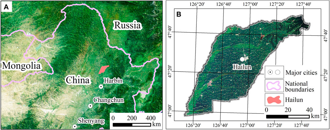
Figure 1. Location (A) and the Landsat-8 true color image of the study area (B).
From late to early stages, stratums in the study area are mainly composed of Quaternary Holocene low washland (sand, mainly covered by grassland), Quaternary Holocene high washland (sand and silt, mainly covered by crop land), Quaternary upper-Pleistocene Guxiangtun Formation (silt and clay, mainly covered by crop land), Quaternary middle-upper-Pleistocene Harbin Formation (silt and clay, mainly covered by crop land), Quaternary middle-Pleistocene Shanghuangshan Formation (silt and clay, mainly covered by crop land), Neogene Sunwu Formation (sand and conglomerate, mainly covered by forest), and upper-Cretaceous Nenjiang Formation (sandstone, mainly covered by forest) (Figure 2A). The magmatic rocks are mainly Permian-Triassic monzonitic granites which are mainly covered by forest (Figure 2A). Elevation in the study area ranges from 150 m to 500 m, and is generally higher in the northeast and lower in the southwest (Figure 2B).
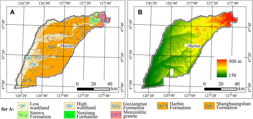
Figure 2. Regional geological map (A) and elevation (B) of the study area.
Figure 3 shows the framework of spatial-temporal analysis of ecological-environmental attributes within different GTEZs, comprising three main parts: data acquisition, information extraction, and statistical analysis.

Figure 3. Workflow of this study.
Regional geological map and high-resolution satellite imagery product were acquired from relevant institute, then the geological map was modified by visual interpretation from high-resolution satellite imagery. Ground survey was conducted in different geological bodies, including four observation points in bedrock outcrops and three drilling points in Quaternary, their vertical compositions were recorded, and the regional geological map was again modified according to the ground survey (Figure 2A). 489 samples of black soil thickness and soil bulk density were collected from Harbin Center for Integrated Natural Resources Survey, CGS (Table 1). Soil parameters might vary a lot within a short range, therefore, these soil data were directly applied to analyzing the statistic characteristics of different GTEZs, rather than interpolated into raster file. Landsat-8 imageries from April to November were collected, which are available at https://earthexplorer.usgs.gov/. For Landsat-8 imageries, it was necessary to ensure that there were no clouds and snow in the study area, and the favorite year was 2022 if possible, imageries from 2020 or 2021 were used when the 2022 images did not meet the requirements. ALOS DEM product was collected from https://search.asf.alaska.edu/, and elevation relief within 1 km2, slope, slope direction, and slope length were then derived from DEM. In addition, air temperature (AT) and total solar radiation (TSR) data were collected and interpolated into raster file to assist the calculation of NPP, the original data could be accessed through Chinese National Meteorological Science Data Center (Table 1).
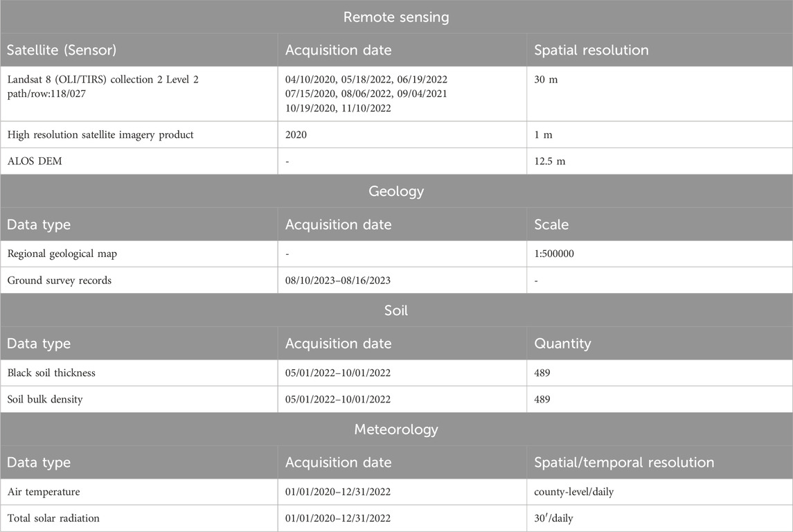
Table 1. Data list of this study.
In this study, the GIS-based analysis method was applied to delineate GTEZs. To be geologically and topographically consistent, the GTEZs were delineated on the basis of regional geological map, elevation, elevation relief, and slope.
In the first step, the formation boundaries in regional geological map were modified through visual interpretation and field survey: ① Quaternary Holocene low washland and Quaternary Holocene high washland tend to change along with the river migration and artificial constructions, so these two formations were re-delineated thoroughly according to interpretation signs (Table 2); ② Quaternary upper-Pleistocene Guxiangtun Formation, Quaternary middle-upper-Pleistocene Harbin Formation, and Quaternary middle-Pleistocene Shanghuangshan Formation share similar composition with different deposition ages, could mainly be separated through Carbon-14 dating, boundaries between them were not distinct to human eyes, so their boundaries were directly deprived from regional geological map; ③As bedrocks, Neogene Sunwu Formation, upper-Cretaceous Nenjiang Formation, and Permian-Triassic monzonitic granites were mainly exposed to land surface in hill or adjacent regions, their boundaries were slightly modified through interpretation signs (Table 2), in addition, three geological bodies of Sunwu Formation conglomerate, Nenjiang Formation sandstone, and monzonitic granite were newly discovered and delineated through field survey.
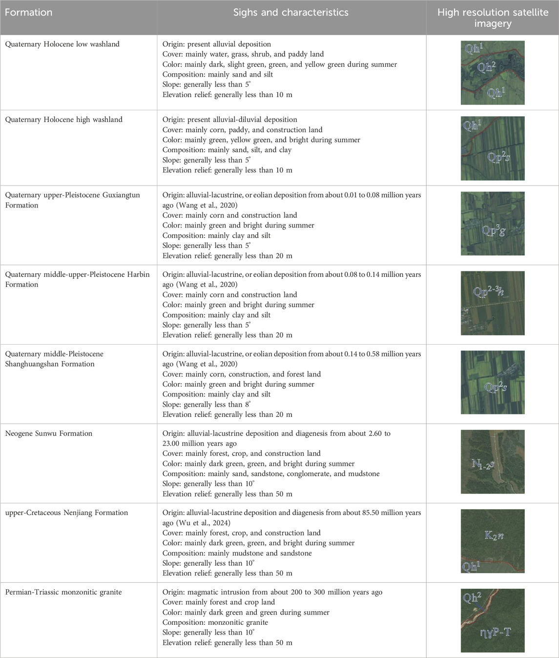
Table 2. Interpretation sighs and characteristics of geological formations.
In the second step, GTEZs were delineated through genesis and qualitative spatial analysis: ① considering the alluvial-diluvial origin at present, Quaternary Holocene washlands were directly converted into sand alluvial plain. ② silt-clay undulating plain was delineated within Quaternary upper-Pleistocene Guxiangtun Formation, Quaternary middle-upper-Pleistocene Harbin Formation, and Quaternary middle-Pleistocene Shanghuangshan Formation from the geological map. Note that the slope of the northeast part of the Quaternary middle-Pleistocene Shanghuangshan Formation is greater than 5°, so this part was excluded from silt-clay undulating plain, and was regarded as sand-conglomerate hill (considering the Sunwu Formation is adjacent and beneath Shanghuangshan Formation). ③ as the terrain within Neogene Sunwu Formation, upper-Cretaceous Nenjiang Formation, and Permian-Triassic monzonitic granites were relatively higher and steeper, they were directly converted into sand-conglomerate hill, sandstone hill, and granite hill zone, respectively.
Landsat 8 OLI/TIRS Collection 2 Level 2 dataset contains the semi-finished products of reflectance and LST, calibration should be applied to these data to eventually obtain the reflectance and LST products:
in Eqs 1, 2 R refers to the reflectance (0–1); DN1∼7 refers to the digital value of band 1∼band 7 from the Landsat 8 OLI Collection 2 Level 2 dataset; LST refers to land surface temperature (K), which could be transformed to Celsius by subtracting 273.15; DN10 refers to the digital value of band 10 from the Landsat 8 TIRS Collection 2 Level 2 dataset.
EVI was processed via band algebra between the reflectance of the near-infrared, red, and blue bands (Garroutte et al., 2016):
in Eq. 3 EVI refers to enhanced vegetation index, RNIR refers to the reflectance of near infrared band (band 5 for Landsat 8), RRed refers to the reflectance of red band (band 4 for Landsat 8), RBlue refers to the reflectance of blue band (band 2 for Landsat 8).
Net primary productivity requires a systematic process and could be derived from the Carnegie-Ames-Stanford Approach (CASA). NDVI, simple ratio for vegetation, total solar radiation (TSR), maximum light use efficiency for vegetation (εmax), daily/monthly mean air temperature (AT), and land surface water index (LSWI) data are typically needed for this approach. The detailed process of CASA is as below (Potter et al., 1993; Zhu et al., 2006; Chandrasekar et al., 2010; Guan et al., 2015; Liang et al., 2019; Yin et al., 2020; Zhang M. et al., 2022):
in Eq. 4 NPP refers to net primary productivity (gC/(m2*month)); FAPAR refers to fraction of absorbed photosynthetically active radiation; PAR refers to photosynthetically active radiation (MJ/(m2*month)); εmax refers to maximum light use efficiency of vegetation (gC/MJ); f (AT1) and f (AT2) refer to effects of temperature stress, f (W) refers to effects of water stress.
in Eqs 5-7 NDVI refers to normalized difference vegetation index; SR refers to simple ratio, SRmin should be set as 1.08, SRmax could be set as 4.14 (evergreen broadleaf forest, and broadleaf forest with groundcover), 6.17 (deciduous broadleaf forest, and mixed forest of broadleaf and needle-leaf), 5.43 (evergreen needle-leaf forest, and deciduous needle-leaf forest), and 5.13 (perennial grassland, broadleaf shrub with grassland, broadleaf shrub with bare soil, tundra, bare soil and desert, and cultivation). When FAPAR exceeds 0.95, the value of FAPAR should be set as 0.95.
in Eq. 8 TSR refers to total solar radiation (MJ/(m2*month)); the factor of 0.5 refers to the fact that approximately half of the incident total solar radiation is within in the PAR wavelength (400∼700 nm).
εmax could be commonly set as 0.389, it also could be set as 0.485(deciduous needle-leaf forest), 0.389(evergreen needle-leaf forest), 0.692(deciduous broadleaf forest), 0.985(evergreen broadleaf forest), 0.475(mixed forest of needle and broadleaf), 0.768(mixed forest of evergreen and deciduous broadleaf), 0.429(broadleaf bush), and 0.542 (grassland, cultivation, and other vegetation).
When the mean monthly air temperature for a month is above −10°C, the f (AT1) of this specific month is set as below:
in Eq. 9 ATopt refers to the mean monthly air temperature at which NDVI reaches its peak during a year. When the mean monthly air temperature for a month is below −10°C, the f (AT1) of this specific month should be set as 0.
When the mean monthly air temperature for a month is within range (ATopt −13, ATopt +10), the f (AT2) of this specific month is set as below:
in Eq. 10 AT refers to the mean monthly air temperature for a month. When the mean monthly air temperature for a month is beyond range (ATopt −13, ATopt +10), the f (AT2) of this specific month is set as 0.5203.
in Eqs 11, 12 LSWI refers to land surface water index; LSWImax refers to the maximum LSWI of a pixel, which is calculated via the maximum value composite method within LSWI time series data; RSWIR refers to the reflectance of shortwave infrared band (band 7 for Landsat 8).
After all the information were extracted, the ecological-environmental attributes within various GTEZs were spatial-temporally analyzed. Among all these attributes, the soil vertical composition records were stored as texts and pictures, so their soil granularities at different depths were qualitatively compared by seven bore-logs. While the soil physical conditions, including black soil thickness and soil bulk density, were stored as tables, due to the strong spatial variability, spatial interpolation among these samples would be unfaithful, so they were qualitatively analyzed by counting the sample amounts within different ranges. On the other hand, elevation relief, slope, slope direction, slope length, LST, EVI, and NPP were stored as raster images, so it would be convenient to quantitatively analyze their GTEZs-related characteristics by a combination of frequency distribution curves, peak values, means, standard deviations (S.D.), medians, and 25%/75% quantiles.
According to the geological and topographical components beneath, five GTEZs were delineated, including: ① sand alluvial plain, where elevation ranges from 150 m to 300 m with the mean of 200 m; ② silt-clay undulating plain, where elevation ranges from 160 m to 350 m with the mean of 230 m; ③ sand-conglomerate hill; ④ sandstone hill; and ⑤ granite hill (Figure 4A). Within the hill region, elevation ranges from 280 m to 500 m with the mean of 350 m. Corresponding to GTEZs, the landforms include alluvial plain, undulating plain, and hill (Figure 4B). The GTEZs in the study area are both relatively diverse and unfragmented, which are suit for spatial-temporal analysis on ecological-environmental attributes.
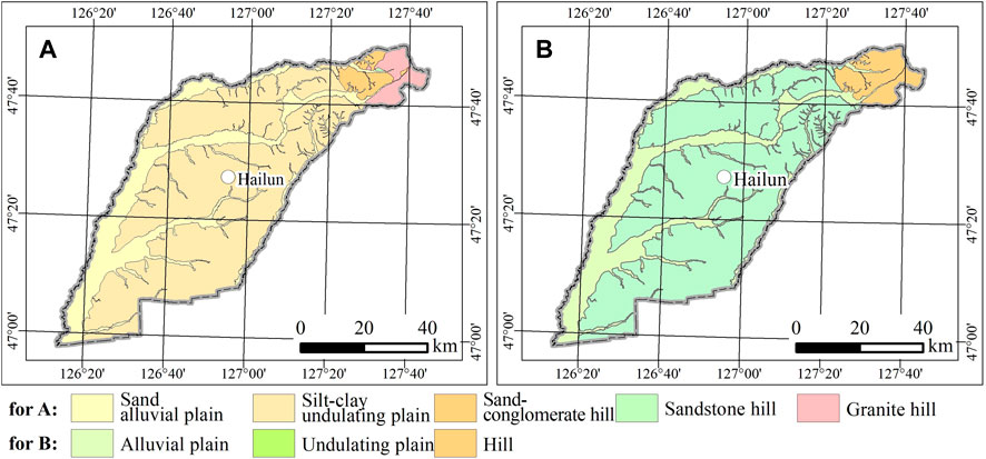
Figure 4. Geological-topographical ecological zones (A), and corresponding landforms (B) of the study area.
Vertical compositions of five GTEZs were observed during the ground survey, the observation points were named as GSP01∼GSP07 (Figure 5). GSP01 was conducted in the sand-conglomerate hill zone, the vertical compositions are sandy silt, pebbly silty sand, and conglomerate from top to bottom. GSP02 was conducted in the sandstone hill zone, the vertical compositions are silty clay, sandy clay, sandy gravel, and sandstone from top to bottom. GSP03 was conducted in the sand-conglomerate hill zone, the vertical compositions are clayey silt, conglomerate, and granite from top to bottom. GSP04 was conducted in the granite hill zone, the vertical compositions are pebbly clayey silt, and granite from top to bottom. GSP05 was conducted in the silt-clay undulating plain zone, the vertical compositions are clayey silt, and silty clay from top to bottom. GSP06 was conducted in the sand-alluvial plain zone, the vertical compositions are clayey silt, silty clay, silty sand, sandy silty clay, and clay from top to bottom. GSP07 was conducted in the sand-alluvial plain zone, the vertical compositions are clayey silt, sandy silt, pebbly sand, sand, and pebbly sand from top to bottom.
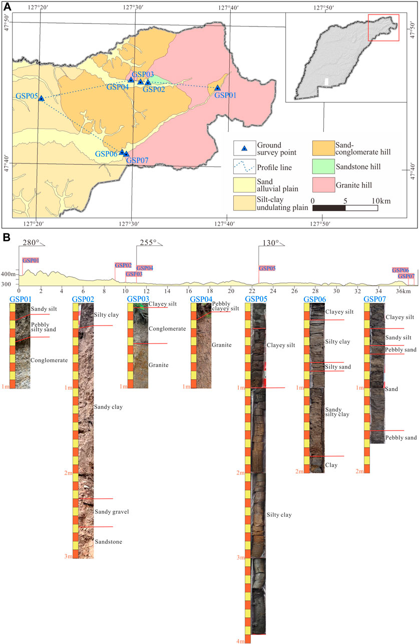
Figure 5. Ground survey point locations (A), and soil vertical compositions (B) of the study area.
As seen from Figure 5, the vertical composition and soil thickness varies between different GTEZs. Sand alluvial plain zone (GSP06, GSP07) possesses thick soil (did not reach the bedrock during ground survey), the soil layer is the most complex, and tend to contain medium-fine grained granule, such as silt, clay, and sand. Silt-clay undulating plain zone (GSP05) possesses very thick soil (did not reach the bedrock during ground survey), the soil layer is the second-most complex, and tend to contain fine grained granule, such as silt and clay. Sand-conglomerate hill zone (GSP01, GSP03) possesses the second-thinnest soil, the soil layer is the second simplest, and tend to contain medium-coarse granule, such as sand and pebble. Sandstone hill zone (GSP02) possesses the relatively thicker soil, the soil layer is relatively more complex, and tend to contain medium granule, such as sand. Granite hill zone (GSP04) possesses the thinnest soil, the soil layer is the simplest, and tend to contain coarse granule, such as pebble and coarse sand.
The black soil thicknesses among GTEZs are relatively distinct. For sand alluvial plain, it mainly ranges from 10 to 60 cm; for silt-clay undulating plain, it also mainly ranges from 10 to 60 cm; for sand-conglomerate hill, it mainly ranges from 10 to 30 cm; there is only one sample in sandstone hill zone, and the black soil thickness is within 30–40 cm; for granite hill, it mainly ranges from 10 to 30 cm (Table 3; Figure 6A). The soil bulk densities among GTEZs are generally similar except granite hill. For sand alluvial plain, it mainly ranges from 1.20 to 1.60 g/cm3; for silt-clay undulating plain, it also mainly ranges from 1.20 to 1.60 g/cm3; for sand-conglomerate hill, it mainly ranges from 1.00 to 1.60 g/cm3; there is only one sample in sandstone hill zone, the soil bulk density is 1.30 g/cm3; and for granite hill, it mainly ranges from 0.60 to 1.40 g/cm3 (Table 3; Figure 6B).
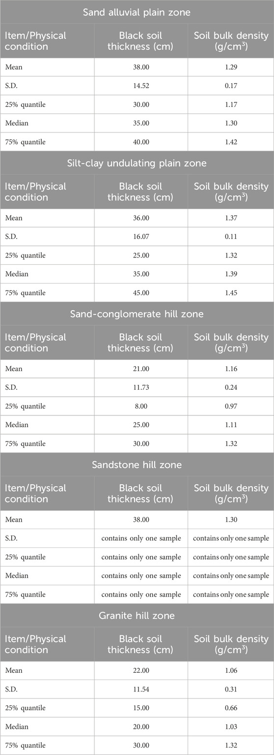
Table 3. Statistical characteristics of soil physical condition.
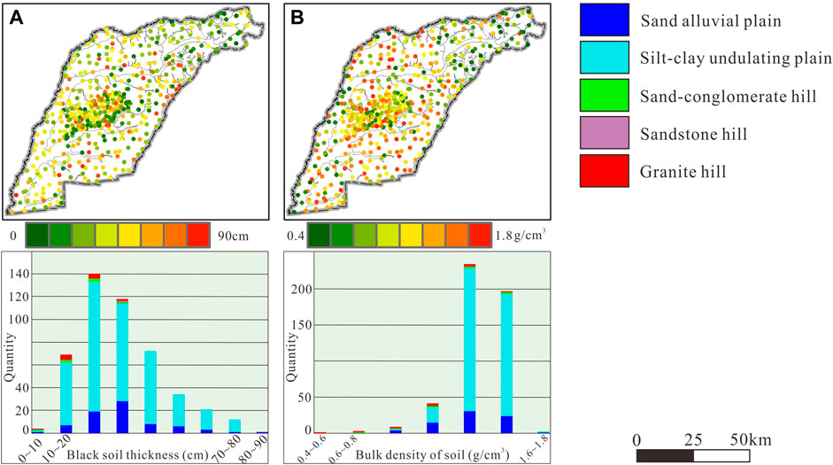
Figure 6. Black soil thickness (A), and soil bulk density (B) of the study area.
The elevation reliefs among GTEZs are distinct from each other. For sand alluvial plain, it mainly ranges from 2 to 10 m, and peaks at about 6 m; for silt-clay undulating plain, it mainly ranges from 3 to 20 m, and peaks at about 6 m; for sand-conglomerate hill, it mainly ranges from 10 to 40 m, and peaks at about 20 m; for sandstone hill, it mainly ranges from 13 to 35 m, and peaks at about 22 m; for granite hill, it mainly ranges from 6 to 50 m, and peaks at about 15 m (Table 4; Figure 7A). Slope directions among GTEZs also show some particularities. Sand alluvial plain and silt-clay undulating plain tend to slant equally among SW, NW, SE, and NE; sand-conglomerate hill tends to slant from NE to SW; sandstone hill tends to slant from N to S; granite hill tends to slant from NW to SE; hill zones generally tend to slant to the west (Table 4; Figure 7C), this might result from the tectonic regime from Mesozoic to Neozoic in Northeastern China (Hu, 2008). Nevertheless, distribution of slopes and slope lengths in GTEZs are generally similar, except that slope exceeding 8° is exclusive to hill zones (Table 4; Figures 7B,D).
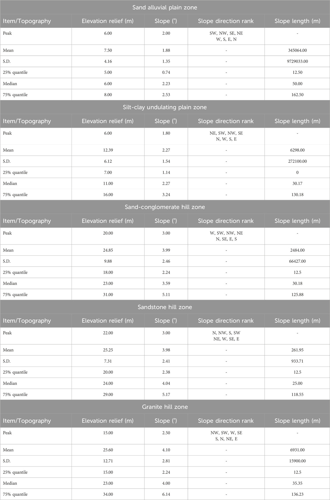
Table 4. Statistical characteristics of topography.
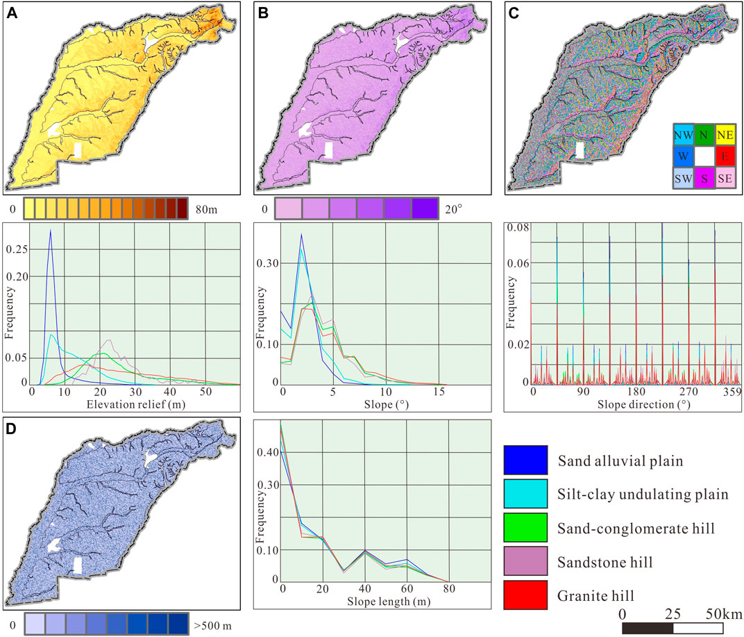
Figure 7. Elevation relief (A), slope (B), slope direction (C), and slope length (D) of the study area.
In April, LST frequency curve is slightly right-skewed normally distributed, and peaks at about 20.00°C; in May, the LST increases, frequency curve is right-skewed normally distributed, and peaks at about 26.50°C; in June, LST continues to increase, frequency curve is slightly right-skewed normally distributed, and peaks at about 33.00°C; in July, LST keeps steady, frequency curve is slightly right-skewed normally distributed, and peaks at about 33.50°C; in August, LST slightly decreases, frequency curve is normally distributed, and peaks at about 29.50°C; in September, LST keeps steady, frequency curve is normally distributed, and peaks at about 28°C; in October, LST decreases significantly, frequency curve is normally distributed, and peaks at about 13.50°C; in November, LST continues to decrease significantly, frequency curve is normally distributed, and peaks at about 5.50°C. From April to November, the frequency curve of monthly LST mean is quasi-normally distributed, and peaks at about 23.50°C; the frequency curve of monthly LST standard deviation (S.D.) is normally distributed, and peaks at about 10.00°C (Table 5; Figures 8, 9).

Table 5. Statistical characteristics of LST (°C).
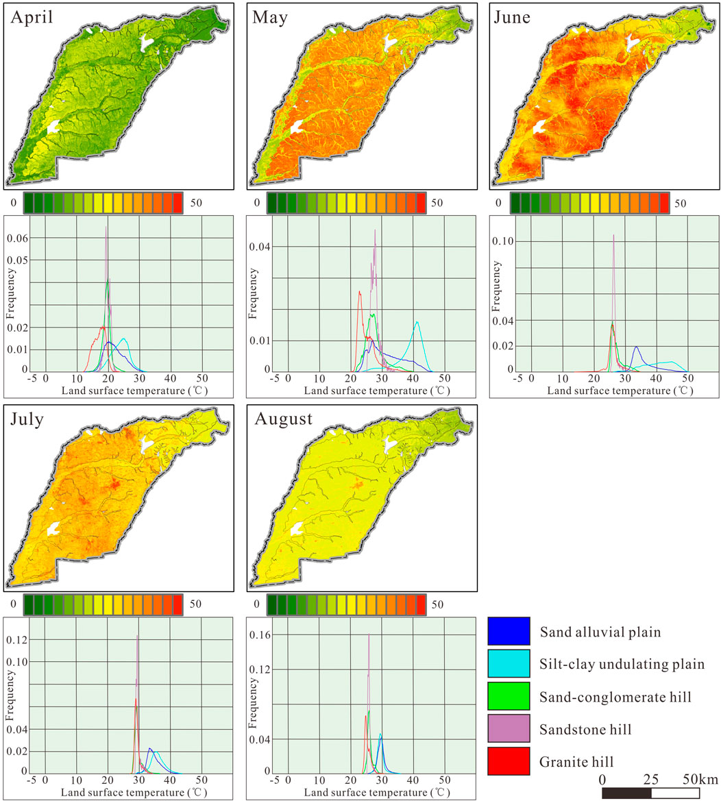
Figure 8. LST from April to August of the study area.
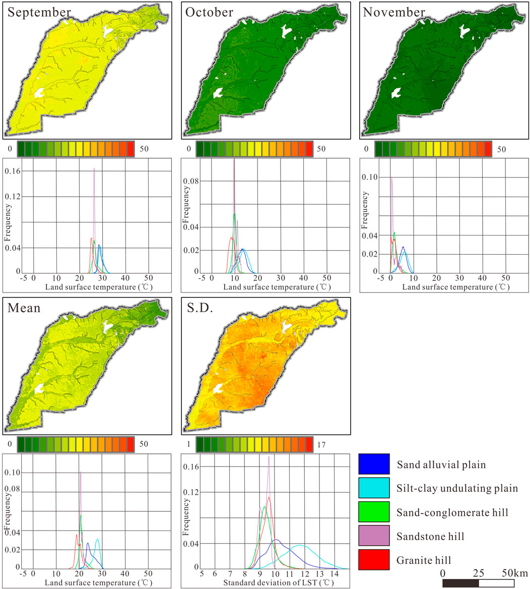
Figure 9. LST from September to November of the study area.
In April, LST frequency curve is slightly left-skewed normally distributed, and peaks at about 25.00°C; in May, LST increases significantly, frequency curve is slightly left-skewed normally distributed, and peaks at about 41.50°C; in June, LST continues to increase slightly, frequency curve is quasi-normally distributed with very gentle slope, and peaks at about 45.00°C; in July, LST decreases slightly, frequency curve is normally distributed, and peaks at about 35.50°C; in August, LST decreases, frequency curve is normally distributed, and peaks at about 29.00°C; in September, LST keeps steady, frequency curve is normally distributed, and peaks at about 28.50°C; in October, LST decreases significantly, frequency curve is normally distributed, and peaks at about 14.00°C; in November, LST continues to decrease, frequency curve is normally distributed, and peaks at about 6.00°C. From April to November, the frequency curve of monthly LST mean is slightly left-skewed normally distributed, and peaks at about 28.00°C; the frequency curve of monthly LST S.D. is right-skewed normally distributed, and peaks at about 11.50°C (Table 5; Figures 8, 9).
In April, LST frequency curve is quasi-normally distributed with steep slope, and peaks at about 20.00°C; in May, LST increases, frequency curve is slightly right-skewed normally distributed, and peaks at about 26.00°C; in June, LST holds steady, frequency curve is right-skewed normally distributed, and peaks at about 26.50°C; in July, LST increases slightly, frequency curve is quasi-normally distributed with steep slope, and peaks at about 29.00°C; in August, LST slightly decreases, frequency curve is quasi-normally distributed with steep slope, and peaks at about 25°C; in September, LST holds steady, frequency curve is slightly right-skewed normally distributed, and peaks at about 26°C; in October, LST decreases significantly, frequency curve is normally distributed, and peaks at about 10.00°C; in November, LST continues to decrease, frequency curve is right-skewed normally distributed, and peaks at about 2.00°C. From April to November, the frequency curve of monthly LST mean is normally distributed, and peaks at about 20.50°C; the frequency curve of monthly LST S.D. is normally distributed, and peaks at about 9.40°C (Table 5; Figures 8, 9).
In April, LST frequency curve is quasi-normally distributed with steep slope, and peaks at about 19.50°C; in May, LST increases, frequency curve is quasi-normally distributed with steep slope, and peaks at about 27.50°C; in June, LST holds steady, frequency curve is quasi-normally distributed with steep slope, and peaks at about 26.50°C; in July, LST increases slightly, frequency curve is quasi-normally distributed with steep slope, and peaks at about 29.50°C; in August, LST slightly decreases, frequency curve is quasi-normally distributed with steep slope, and peaks at about 25.50°C; in September, LST holds steady, frequency curve is quasi-normally distributed with steep slope, and peaks at about 26.00°C; in October, LST decreases significantly, frequency curve is quasi-normally distributed with steep slope, and peaks at about 10.00°C; in November, LST continues to decrease, frequency curve is quasi-normally distributed with steep slope, and peaks at about 1.00°C. From April to November, the frequency curve of monthly LST mean is quasi-normally distributed, and peaks at about 20.00°C; the frequency curve of monthly LST S.D. is bimodally distributed, and peaks at about 9.60°C and 9.00°C (Table 5; Figures 8, 9).
In April, LST frequency curve is slightly left-skewed normally distributed, and peaks at about 18.00°C; in May, LST increases, frequency curve is right-skewed normally distributed, and peaks at about 23.00°C; in June, LST keeps steady, frequency curve is normally distributed, and peaks at about 26.50°C; in July, LST increases slightly, frequency curve is quasi-normally distributed with steep slope, and peaks at about 29.00°C; in August, LST slightly decreases, frequency curve is quasi-normally distributed with steep slope, and peaks at about 24.50°C; in September, LST holds steady, frequency curve is quasi-normally distributed with steep slope, and peaks at about 24.50°C; in October, LST decreases significantly, frequency curve is normally distributed, and peaks at about 8.50°C; in November, LST continues to decrease, frequency curve is quasi-normally distributed with faintly double-peaks, and generally peaks at about 1.00°C. From April to November, the frequency curve of monthly LST mean is quasi-normally distributed with faintly double-peaks, and primarily peaks at about 19.00°C; the frequency curve of monthly LST S.D. is normally distributed, and peaks at about 9.60°C (Table 5; Figures 8, 9).
In April, EVI frequency curve is normally distributed, and peaks at about 0.11; in May, EVI holds steady, frequency curve is slightly right-skewed normally distributed, and peaks at about 0.09; in June, EVI increases, frequency curve is slightly right-skewed normally distributed, and peaks at about 0.19; in July, EVI increases significantly, frequency curve is left-skewed normally distributed, and peaks at about 0.60; in August, EVI continues to increase, frequency curve is normally distributed with a second peak on the right slope, and peaks primarily at about 0.68; in September, EVI decreases, frequency curve is normally distributed, and peaks at about 0.48; in October, EVI decreases significantly, frequency curve is bimodally distributed, and peaks at about 0.19 and 0.10; in November, EVI continues to decrease, frequency curve is quasi-normally distributed with two peaks, which are 0.12 and 0.08. From April to November, the frequency curve of monthly EVI mean is normally distributed, and peaks at about 0.30; the frequency curve of monthly EVI S.D. is left-skewed normally distributed, and peaks at about 0.24 (Table 6; Figures 10, 11).

Table 6. Statistical characteristics of EVI.
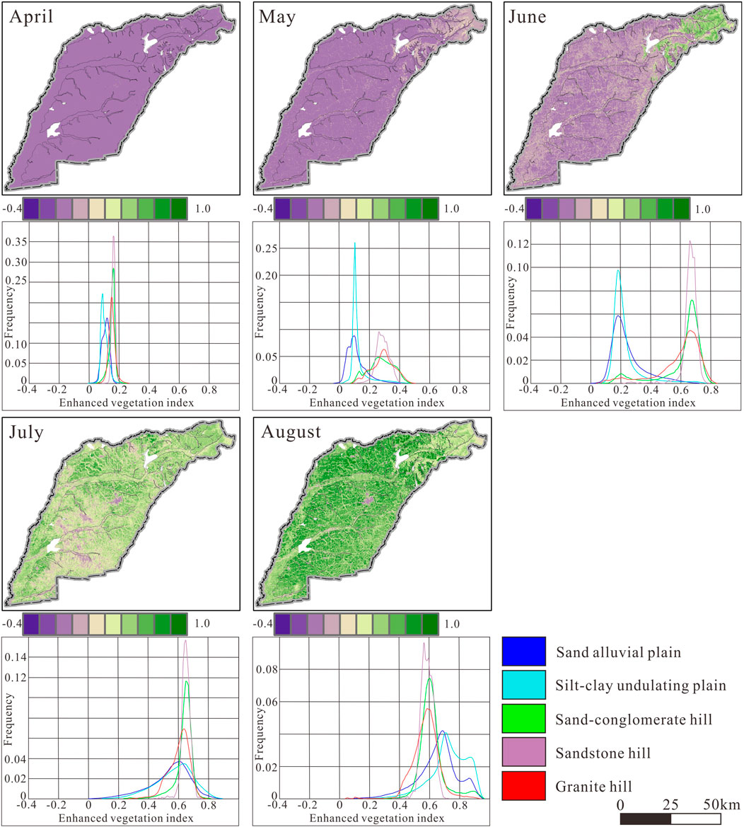
Figure 10. EVI from April to August of the study area.
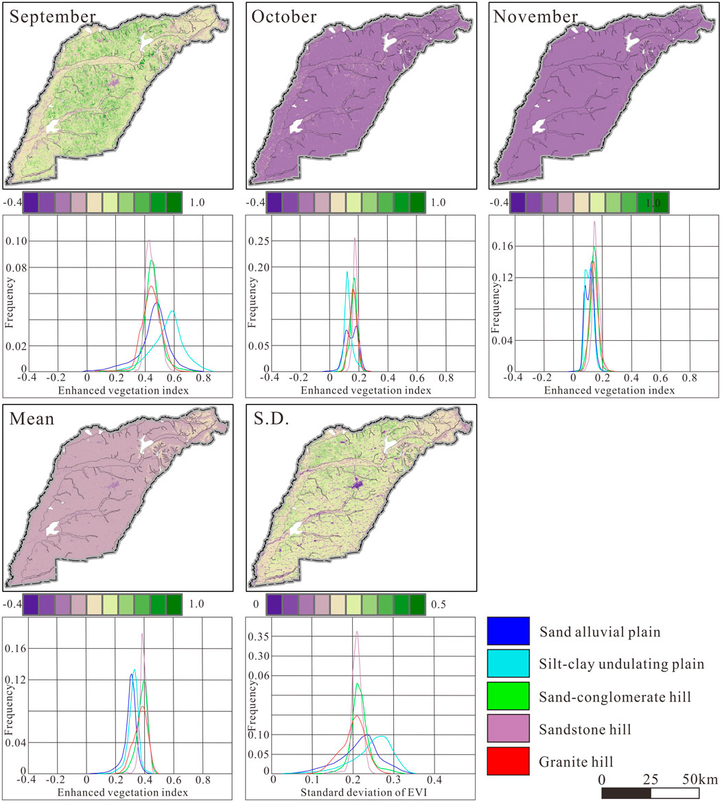
Figure 11. EVI from September to November of the study area.
In April, EVI frequency curve is normally distributed with steep slope, and peaks at about 0.08; in May, EVI holds steady, frequency curve is normally distributed with steep slope, and peaks at about 0.11; in June, EVI slightly increases, frequency curve is normally distributed, and peaks at about 0.19; in July, EVI increases significantly, frequency curve is left-skewed normally distributed, and peaks at about 0.63; in August, EVI continues to increase, frequency curve is bimodally distributed, and peaks at about 0.71 and 0.83; in September, EVI decreases, frequency curve is normally distributed, and peaks at about 0.59; in October, EVI decreases significantly, frequency curve is normally distributed, and peaks at about 0.11; in November, EVI holds steady, frequency curve is quasi-normally distributed with two peaks at top, and generally peaks at about 0.10. From April to November, the frequency curve of monthly EVI mean is normally distributed, and peaks at about 0.32; the frequency curve of monthly EVI S.D. is left-skewed normally distributed, and peaks at about 0.28 (Table 6; Figures 10, 11).
In April, EVI frequency curve is quasi-normally distributed with steep slope, and peaks at about 0.16; in May, EVI increases, frequency curve is bimodally distributed, and peaks primarily at about 0.26 and 0.12; in June, EVI increases significantly, frequency curve is slightly left-skewed normally distributed, and peaks at about 0.68; in July, EVI increase very slightly, frequency curve is normally distributed with steep slope, and peaks at about 0.64; in August, EVI decrease slightly, frequency curve is normally distributed, and peaks at about 0.60; in September, EVI decreases, frequency curve is normally distributed, and peaks at about 0.44; in October, EVI decreases significantly, frequency curve is normally distributed with steep slope, and peaks at about 0.18; in November, EVI holds steady, frequency curve is normally distributed with steep slope, and generally peaks at about 0.14. From April to November, the frequency curve of monthly EVI mean is slightly left-skewed normally distributed, and peaks at about 0.40; the frequency curve of monthly EVI S.D. is normally distributed, and peaks at about 0.21 (Table 6; Figures 10, 11).
In April, EVI frequency curve is normally distributed with steep slope, and peaks at about 0.16; in May, EVI increases, frequency curve is quasi-normally distributed, and peaks at about 0.26; in June, EVI increases significantly, frequency curve is normally distributed, and peaks at about 0.67; in July, EVI keeps steady, frequency curve is normally distributed with steep slope, and peaks at about 0.63; in August, EVI decreases, frequency curve is normally distributed with faintly two peaks at top, and generally peaks at about 0.56; in September, EVI continues to decrease, frequency curve is normally distributed, and peaks at about 0.42; in October, EVI decreases significantly, frequency curve is normally distributed with steep slope, and peaks at about 0.19; in November, EVI holds steady, frequency curve is normally distributed with steep slope, and peaks at about 0.15. From April to November, the frequency curve of monthly EVI mean is normally distributed with steep slope, and peaks at about 0.39; the frequency curve of monthly EVI S.D. is normally distributed with steep slope, and peaks at about 0.21 (Table 6; Figures 10, 11).
In April, EVI frequency curve is normally distributed with steep slope, and peaks at about 0.15; in May, EVI increases, frequency curve is quasi-normally distributed, and peaks at about 0.30; in June, EVI increases significantly, frequency curve is left-skewed normally distributed, and peaks at about 0.67; in July, EVI keeps steady, frequency curve is left-skewed normally distributed, and peaks at about 0.62; in August, EVI decrease very slightly, frequency curve is normally distributed, and peaks at about 0.60; in September, EVI continues to decrease, frequency curve is normally distributed, and peaks at about 0.44; in October, EVI decreases significantly, frequency curve is normally distributed, and peaks at about 0.17; in November, EVI holds steady, frequency curve is normally distributed, and peaks at about 0.13. From April to November, the frequency curve of monthly EVI mean is slightly left-skewed normally distributed, and peaks at about 0.39; the frequency curve of monthly EVI S.D. is also slightly left-skewed normally distributed, and peaks at about 0.21 (Table 6; Figures 10, 11).
In April, NPP frequency curve is normally distributed with steep slope, and peaks at about 3.00 gC/(m2*month); in May, NPP increases slightly, frequency curve is right-skewed quasi-normally distributed, and peaks at about 7.00 gC/(m2*month); in June, NPP increases significantly, frequency curve is uniformly distributed from 10.00 to 160.00 gC/(m2*month) with a minor peak at 140.00 gC/(m2*month); in July, NPP increases significantly, frequency curve is left-skewed quasi-normally distributed, and peaks at about 135.00 gC/(m2*month); in August, NPP continues to increase, frequency curve is bimodally distributed with steep slope, and peaks at about142.00 and 148.00 gC/(m2*month); in September, NPP decreases, frequency curve is left-skewed normally distributed, and peaks at about 101.00 gC/(m2*month); in October, NPP decreases significantly, frequency curve is normally distributed with steep slope, and peaks at about 3.00 gC/(m2*month); in November, NPP generally continues to decrease to 0 gC/(m2*month). From April to November, the frequency curve of monthly NPP mean is bimodally distributed, and peaks at about 68.00 and 51.00 gC/(m2*month); the frequency curve of monthly NPP S.D. is also bimodally distributed, and peaks at about 57.00 and 62.00 gC/(m2*month); the frequency curve of yearly total NPP is still bimodally distributed, and peaks at about 545.00 and 415.00 gC/(m2*year) (Table 7; Figures 12, 13).

Table 7. Statistical characteristics of NPP (gC×m-2×month-1).
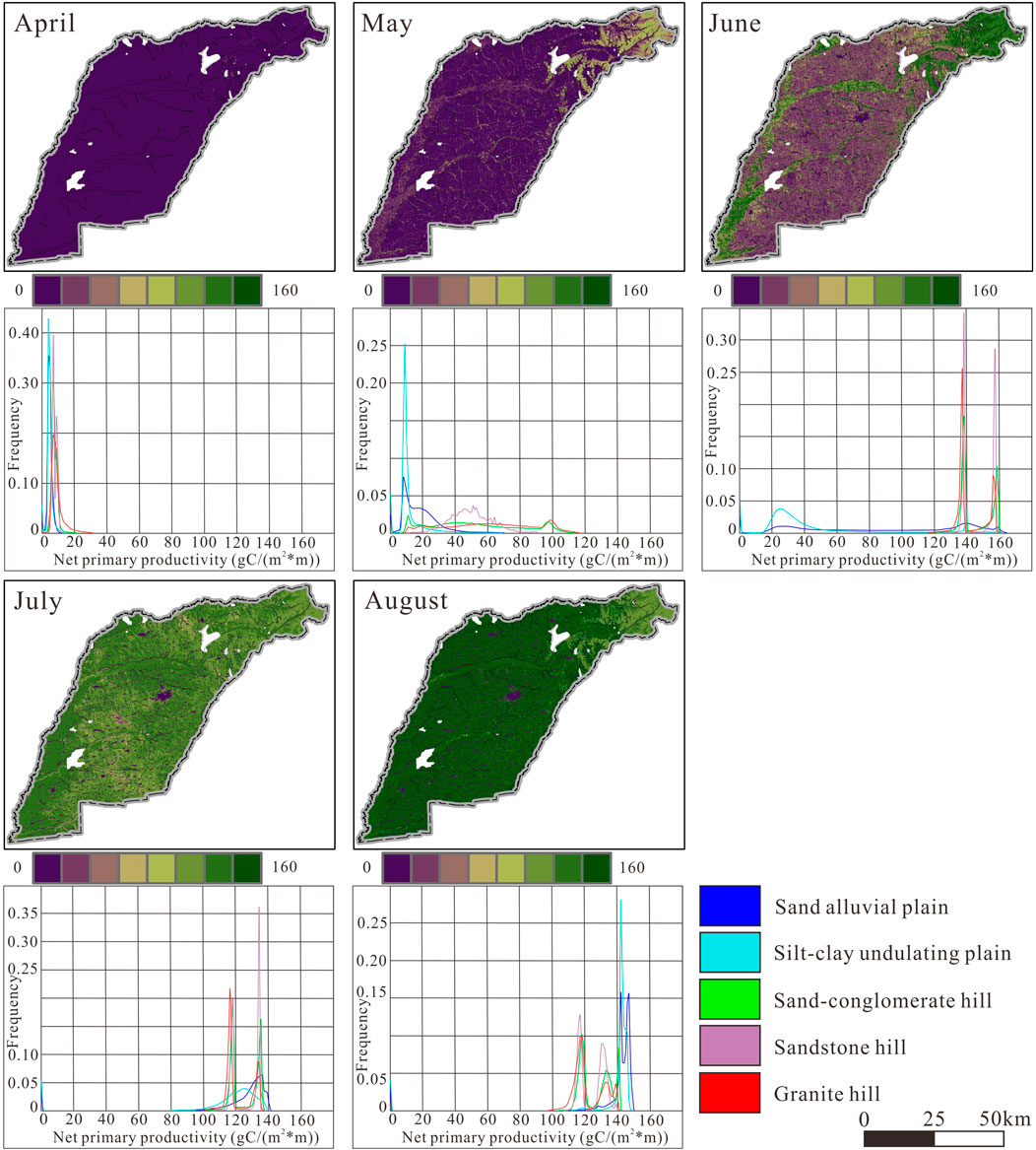
Figure 12. NPP from April to August of the study area.

Figure 13. NPP from September to November of the study area.
In April, NPP frequency curve is quasi-normally distributed with steep slope, and peaks at about 3.00 gC/(m2*month); in May, NPP increases slightly, frequency curve is normally distributed with steep slope, and peaks at about 9.00 gC/(m2*month); in June, NPP increases significantly, frequency curve is right-skewed normally distributed, and peaks at about 25.00 gC/(m2*month); in July, NPP increases significantly, frequency curve is left-skewed normally distributed, and peaks at about 127.00 gC/(m2*month); in August, NPP continues to increase, frequency curve is quasi-normally distributed with steep slope, and peaks at about 142.00 gC/(m2*month); in September, NPP decreases, frequency curve is quasi-normally distributed with two peaks at top, which are 101.00 and 106.00 gC/(m2*month); in October, NPP continues to decrease significantly, frequency curve is quasi-normally distributed with steep slope, and peaks at about 3.00 gC/(m2*month); in November, NPP generally continues to decrease to 0 gC/(m2*month). From April to November, the frequency curve of monthly NPP mean is quasi-normally distributed, and peaks at about 52.00 gC/(m2*month); the frequency curve of monthly NPP S.D. is normally distributed, and peaks at about 56.00 gC/(m2*month); the frequency curve of yearly total NPP is also normally distributed, and peaks at about 410.00 gC/(m2*year) (Table 7; Figures 12, 13).
In April, NPP frequency curve is quasi-normally distributed with steep slope, and peaks at about 7.00 gC/(m2*month); in May, NPP increases significantly, frequency curve is uniformly distributed with two minor peaks at about 11.00 and 98.00 gC/(m2*month); in June, NPP increases significantly, frequency curve is bimodally distributed, and peaks at about 139.00 and 159.00 gC/(m2*month); in July, NPP decreases slightly, frequency curve is also bimodally distributed, and peaks at about 119.00 and 135.00 gC/(m2*month); in August, NPP keeps steady, frequency curve is trimodally distributed, and peaks at about 118.00, 141.00, and 132.00 gC/(m2*month); in September, NPP decreases significantly, frequency curve is bimodally distributed, and peaks at about 79.00 and 88.00 gC/(m2*month); in October, NPP continues to decrease significantly, frequency curve is quasi-normally distributed with steep slope, and peaks at about 5.00 gC/(m2*month); in November, NPP generally continues to decrease to 0 gC/(m2*month). From April to November, the frequency curve of monthly NPP mean is quasi-normally distributed, and peaks at about 70.00 gC/(m2*month); the frequency curve of monthly NPP S.D. is bimodally distributed, and peaks at about 53.00 and 60.00 gC/(m2*month); the frequency curve of yearly total NPP is quasi-normally distributed, and peaks at about 560.00 gC/(m2*year) (Table 7; Figures 12, 13).
In April, NPP frequency curve is bimodally distributed with steep slope, and peaks at about 7.00 and 10.00 gC/(m2*month); in May, NPP increases significantly, frequency curve is quasi-normally distributed, and peaks at about 50.00 gC/(m2*month); in June, NPP continues to increase significantly, frequency curve is bimodally distributed, and peaks at about 139.00 and 158.00 gC/(m2*month); in July, NPP decreases slightly, frequency curve is also bimodally distributed, and peaks at about 134.00 and 119.00 gC/(m2*month); in August, NPP keeps steady, frequency curve is still bimodally distributed, and peaks at about 117.00 and 130.00 gC/(m2*month); in September, NPP decreases significantly, frequency curve is still bimodally distributed, and peaks at about 78.00 and 88.00 gC/(m2*month); in October, NPP continues to decrease significantly, frequency curve is quasi-normally distributed with steep slope, and peaks at about 5 gC/(m2*month); in November, NPP generally continues to decrease to 0 gC/(m2*month). From April to November, the frequency curve of monthly NPP mean is bimodally distributed, and peaks at about 71.00 and 62.00 gC/(m2*month); the frequency curve of monthly NPP S.D. is also bimodally distributed, and peaks at about 53.00 and 60.00 gC/(m2*month); the frequency curve of yearly total NPP is still bimodally distributed, and peaks at about 570.00 and 505.00 gC/(m2*year) (Table 7; Figures 12, 13).
In April, NPP frequency curve is quasi-normally distributed with steep slope, and peaks at about 7.00 gC/(m2*month); in May, NPP increases significantly, frequency curve is uniformly distributed from 15.00 to 120.00 gC/(m2*month), a minor peak could be seen at about 98.00 gC/(m2*month); in June, NPP continues to increase significantly, frequency curve is bimodally distributed, and peaks at about 138.00 and 157.00 gC/(m2*month); in July, NPP decreases slightly, frequency curve is also bimodally distributed, and peaks at about 118.00 and 134.00 gC/(m2*month); in August, NPP keeps steady, frequency curve is trimodally distributed, and peaks at about 117.00, 131.00, and 139.00 gC/(m2*month); in September, NPP decreases significantly, frequency curve is quasi-normally distributed with a second peak at right, and primarily peaks at about 82.00 gC/(m2*month); in October, NPP continues to decrease significantly, frequency curve is quasi-normally distributed with steep slope, and peaks at about 5.00 gC/(m2*month); in November, NPP generally continues to decrease to 0 gC/(m2*month). From April to November, the frequency curve of monthly NPP mean is quasi-normally distributed, and peaks at about 70.00 gC/(m2*month); the frequency curve of monthly NPP S.D. is bimodally distributed, and peaks at about 53.00 and 60.00 gC/(m2*month); the frequency curve of yearly total NPP is left-skewed quasi-normally distributed, and peaks at about 560.00 gC/(m2*year) (Table 7; Figures 12, 13).
The formation of soil is mainly affected by parent material, climate, topography, organisms, and time (Mapelli et al., 2012), among which the parent material directly determines the primary soil structure, topography indirectly affects soil material migration and energy redistribution (Liu, 2018). Soil vertical compositions and physical conditions act as examples of soil diversities among different GTEZs (Table 3; Figures 5, 6).
Sand alluvial plain zone is topographically adjacent to rivers, the soil composition strongly depends on alluvial-diluvial parent materials derived from rivers and floods (El Hourani and Broll, 2021). The soil layers and granule sizes in sand alluvial plain zone are mainly related to sediment transportation and deposition, in this study, the complex soil layers and medium-fine granules (Figure 5) are due to the volatile historical flow regime and fluvial environment (Gerrard, 1987; Boettinger, 2005). Silt-clay undulating plain zone is topographically in the transitional zone between alluvial plain and hills, and soil composition is materially related to the Shanghuangshan Formation, Guxiangtun Formation, and Harbin Formation, their thick-bedded yellow-tawny fine granules (Figure 5) were derived from alluvial-lacustrine, or eolian deposition facies, and pollens indicate a dry-cold climate background (Wang, 2012). Black soil is generally derived from sandy-silty sediments (Andreeva et al., 2011), and soil bulk density is related to organic matter content, land use, soil genus and topography (Li et al., 2019). Compared to three hill zones, the two plain zones possess thicker black soil and higher bulk density (Table 3; Figure 6), hill zones with forest could accumulate more organic matters and coarse granules with more porosity in the surface soil, which would result in lower bulk density.
At present, the main geological processes in the hill zones are weathering and residual-slope deposition. Sand-conglomerate hill zone possesses the second-thinnest soil, the second simplest soil layers, and the second coarsest soil granules; sandstone hill zone possesses the relatively thicker soil, the relatively-more complex soil layers, and medium soil granules; granite hill zone possesses the thinnest soil, the simplest soil layers, and the coarsest soil granules (Figure 5). Soil parameters might differ within a local scale as a reflection of rock and topographical diversity (Fonseca et al., 2021). Table 4 and Figure 7 shows that these three hill zones generally share similar elevation relief, slope and relatively particular slope direction, bed rock and slope direction could be the main factor that causes difference in rock weathering rate and soil formation rate (Abe et al., 2019), sedimentary rocks generally weather faster than igneous and metamorphic rocks (Evans et al., 2021). The soil parameter differences between three hill zones are the combined outcomes of petrogenesis, minerals, granule sizes, cements diversities, and slope directions among conglomerate, sandstone, and granite.
land surface parameters in different GTEZs tend to show their particular patterns for some possible reasons. The sand alluvial plain zone typically contains grassland and cultivated land, and displays relatively moderate monthly variations of EVI, LST, and NPP as season changes (Table 5–7; Figure 8–13). In April and May, EVI is mainly within 0.05 and 0.25, indicating the scattered existence of grassland, LST increases as air temperature rises, vegetation activity is restrained by air temperature, and NPP mainly ranges from 0 to 30.00 gC/(m2*m). When comes to June, EVI is mainly within 0.10 and 0.40, this is related to landcovers, grasses and crops in Heilongjiang Province start to thrive in June and July, respectively (Hu et al., 2019). Since air temperature keeps rising, LST also continues to increase, NPP in some positions could be around 140.00 gC/(m2*m). In July, due to the flourish of grass and crops, the general EVI increases significantly, and is mainly within 0.40 and 0.70, LST keeps unchanged when monthly air temperature reaches its peak, NPP also increases significantly to the range of 120.00 and 140.00 gC/(m2*m). In August, EVI continues to increase and reaches peak, and is mainly within 0.50 and 0.85, LST slightly decreases along with the air temperature’s decline, NPP also continues to increase and reaches peak, and mainly ranges from 140.00 to 150.00 gC/(m2*m). From September to November, since vegetation fades and air temperature keeps declining, the EVI, LST, and NPP maintain downward trends.
Benefiting from its relatively higher elevation (without the frequent threat of flood) and gentle slope, silt-clay undulating plain zones are highly cultivated for crops and exploited for construction, and displays significant monthly variations of EVI, LST, and NPP as season changes (Table 5–7; Figure 8–13). In April and May, EVI is mainly under 0.20, LST of the nearly-bare cultivated lands increases as air temperature rises, the NPP is mainly under 20.00 gC/(m2*m). In June, crops start to sprout, EVI is mainly within 0.10 and 0.30, LST continues to slightly increase with more spatial varieties, which might be caused by the uneven growth of crops, NPP is mainly around 19.00 and 40.00 gC/(m2*m). When comes to July, the general EVI increases significantly, and is mainly within 0.40 and 0.70. LST decreases significantly despite that the monthly air temperature reaches its peak, this could be explained that crops become flourishing in July, and LST reflects the temperature of crop canopy, which is dramatically pulled down by vegetation transpiration (Bramley et al., 2022). NPP also increases significantly to the range of 110.00 and 138.00 gC/(m2*m). In August, EVI continues to increase and reaches peak, and is mainly within 0.60 and 0.85, LST slightly decreases along with the air temperature’s decline and the flourish of crops, NPP also continues to increase and reaches peak, and mainly ranges from 140.00 to 148.00 gC/(m2*m). From September to November, since the crop harvest and air temperature’s declining, the EVI, LST, and NPP of silt-clay undulating plain zone also show downward trends.
The seasonal EVI, LST, and NPP frequency curves of sand-conglomerate hill zone, sandstone hill zone, and granite hill zone are generally similar. Minor diversities among three zones might be caused by spatial differences of geology, geologically-derived soil parameter, geologically-derived ground water condition (Costa et al., 2017; Sabathier et al., 2021), and tree species, forest with taller trees tends to present greater net cooling effect (Zhang Z. et al., 2022; Shaik et al., 2023). Landcovers of these three zones are dominated by mixed forest of broadleaf and needle-leaf, and displays relatively slight monthly variations of EVI, LST, and NPP as season changes (Table 5–7; Figure 8–13). In April, due to the deciduous forest, EVI is mainly under 0.20, the NPP is correspondingly under 20.00 gC/(m2*m). When comes to May, forest starts to sprout, EVI is mainly within 0.10 and 0.40, LST increases as air temperature rises, and NPP increases with more spatial varieties, which might be caused by uneven distribution of broad-leaf and needle-leaf forest. In June, forest flourishes, EVI is mainly within 0.60 and 0.75 and reaches peak, LST holds stable under the combined influence of air temperature and vegetation transpiration, NPP increases significantly with the flourish forest and proper air temperature, and is around 138.00 and 158.00 gC/(m2*m). In July, EVI keeps steady, and is mainly within 0.50 and 0.70, LST slightly increases and reaches peak, this might be due to the minor decline of forest growth and air temperature’s peak in July. As the consequent of air temperature rising and vegetation condition, NPP decreases to around 118.00 and 135.00 gC/(m2*m). Entering August, EVI and LST slightly decrease, but NPP fluctuates or keeps stable, this phenomenon might be because the air temperature lowers down to an optimal range for forest. In September, due to seasonal change, EVI continues decrease, but LST holds stable, NPP correspondingly decreases gradually. From October to November, the changing season is in dominan, EVI, LST, and NPP decrease significantly along with air temperature’s decline. During June and August, the NPP frequency curves are bimodally or trimodally distributed, whereas the corresponding EVI frequency curves are normally distributed, this might be because the NPP is also dependent on the humidity and air temperature, while humidity and air temperature could vary at different slopes and slope directions.
As seen from the spatial-temporal patterns of soil and land surface parameters in different GTEZs, the combination of geology and topography contribute a lot to the spatial-temporal pattern of ecological-environmental attributes in a region. Lithological condition could determine the weathering resistance and parent materials, which affects soil composition and formation rate, and topographical condition could influent the migration of parent materials, which affects soil vertical composition and physical conditions. Furthermore, topography and the geological-topographically-driven soil parameters would limit vegetation growth and human activities, then determine the landcover, whose phenology could interact with ecology (Snyder et al., 2019; Ranjbar et al., 2020), and is as essential as topography to the land surface parameters. Ecological zoning from the perspective of geology and topography is helpful to understanding the primary mechanism of ecological environmental processes.
According to the spatial-temporal patterns of ecological-environmental parameters in different GTEZs, there are several advices for ecological management: ① Hill zones possess the thinnest soil thickness (Figure 5) and the highest total yearly NPP (Table 7), and recover the slowest from damage and contribute the most to carbon neutrality (Wen et al., 2023), so disturbance to hill zones should be avoided. ② Hill zones, with the most seasonally stable ecological-environmental attributes, are ideal habitats for wild animals. However, with relatively moderate slope (Table 4; Figure 7B), hill zone is also available for cultivation, this may rise the risk of human-wild animal conflict, so the possible unpermitted assart in hill zones should be constantly monitored. ③ The silt-clay undulating plain zone is nearly bare land from April to June, while precipitation is concentrated from May to September, and tends to cause soil loss and erosion gullies. Planting shrub on the bottom of erosion gullies is recommended, and it is beneficial to inhibiting erosion gully extension and promoting landscape diversity without occupying crop land.
There are also several limitations to this study: (1) the study area is a temperate region mainly covered by forest, cultivated land, and grassland, and the land surface is widely covered by snow from late November to early April. Besides, vegetation transpiration produces considerable water vapor or clouds during summer, which would limit the availability of optical images. A particular sensor (Landsat 8 OLI/TIRS in this study) generally could not provide qualified images from April to November in one particular year, resulting the images applied for monthly patterns in this study are within 2020 and 2022. (2) The outcrops of bedrock (especially sandstone of the Nenjiang Formation) in the hilly region are relatively scarce, which limits the amount of ground survey points and representativeness of soil parameters, future observations in similar areas should be used to conduct more comprehensive discussion.
The study area, belonging to the transitional zone between plain and mountain range, contains both plains and hills with crops and forests. The comprehensive application of geology, topography, soil composition, soil physical condition, LST, EVI, and NPP has preliminarily revealed the spatial-temporal patterns of ecological-environmental attributes within different GTEZs. Under the integrated effect of geology, topography, and corresponding human activities, the plain zones mainly possess layered thick soil with fine-medium grained granule and higher bulk density. As season changes, bare lands in plain zones start to transfer to crop lands in June, and the crops flourish the most in August with the highest monthly NPP. The hill zones, on the other hand, possess relatively thin soil with medium-coarse granule and lower bulk density. As season changes, green on the hill starts to merge in May, and flourish the most in June and July, and have the highest yearly total NPP, which highlights the vulnerability to disturbance and significance to carbon neutrality. Geological and topographical conditions are fundamental to soil parameters by affecting the provenance, type, and distribution of parent materials; topography and the geological-topographically-related soil parameters are essential to land surface parameters by affecting the landcover. Ecological zoning would help understand the ecological-environmental conditions more essentially when considering geological and topographical conditions, which could primarily affect the ecological-environmental process.
The original contributions presented in the study are included in the article/Supplementary material, further inquiries can be directed to the corresponding author.
ZC: Conceptualization, Data curation, Formal Analysis, Funding acquisition, Investigation, Methodology, Project administration, Software, Visualization, Writing–original draft, Writing–review and editing. TL: Conceptualization, Funding acquisition, Project administration, Writing–review and editing. KY: Funding acquisition, Methodology, Project administration, Writing–review and editing. YL: Methodology, Software, Visualization, Writing–review and editing.
The author(s) declare that financial support was received for the research, authorship, and/or publication of this article. This study was funded by Harbin Center for Integrated Natural Resources Survey, China Geological Survey (No. DD20211589) and Northeast Geological S&T Innovation Center of China Geological Survey (No. QCJJ2022-6).
The authors thank reviewers for their constructive comments and instructions, and editors for their elaborative, patient assistances. The authors would also like to acknowledge USGS for providing access to Landsat imagery, NASA for providing access to DEM products, and other institutions for providing meteorological, high resolution satellite imagery, geological map, and soil parameter data, which are all of great help.
The authors declare that the research was conducted in the absence of any commercial or financial relationships that could be construed as a potential conflict of interest.
All claims expressed in this article are solely those of the authors and do not necessarily represent those of their affiliated organizations, or those of the publisher, the editors and the reviewers. Any product that may be evaluated in this article, or claim that may be made by its manufacturer, is not guaranteed or endorsed by the publisher.
Abe, S. S., Harada, T., Okumura, H., and Wakatsuki, T. (2019). Comparing rates of rock weathering and soil formation between two temperate forest watersheds differing in parent rock and vegetation type. Jpn. Agric. Res. Q. 53 (3), 169–179. doi:10.6090/jarq.53.169
Alavi Panah, S. K., Kiavarz Mogaddam, M., and Karimi Firozjaei, M. (2017). Monitoring spatiotemporal changes of heat island in Babol city due to land use changes. Int. Archives Photogrammetry, Remote Sens. Spatial Inf. Sci., 17–22. doi:10.5194/isprs-archives-XLII-4-W4-17-2017
Amin, M. E. S., Mohamed, E. S., Belal, A. A., Jalhoum, M. E. M., Abdellatif, M. A., Nady, D., et al. (2022). Developing spatial model to assess agro-ecological zones for sustainable agriculture development in MENA region: case study Northern Western Coast, Egypt. Egypt. J. Remote Sens. Space Sci. 25 (1), 301–311. doi:10.1016/j.ejrs.2022.01.014
Andreeva, D. B., Leiber, K., Glaser, B., Hambach, U., Erbajeva, M., Chimitdorgieva, G. D., et al. (2011). Genesis and properties of black soils in Buryatia, southeastern Siberia, Russia. Quat. Int. 243 (2), 313–326. doi:10.1016/j.quaint.2010.12.017
Bai, X., Zhao, W., Luo, W., and An, N. (2024). Effect of climate change on the seasonal variation in photosynthetic and non-photosynthetic vegetation coverage in desert areas, Northwest China. Catena 239, 107954. doi:10.1016/j.catena.2024.107954
Bian, J., ·Chen, W., and Zeng, J. (2023). Ecosystem services, landscape pattern, and landscape ecological risk zoning in China. Environ. Sci. Pollut. Res. 30, 17709–17722. doi:10.1007/s11356-022-23435-5
Boettinger, J. L. (2005). “Alluvium and alluvial soils,” in Encyclopedia of soils in the environment. Editor D. Hillel (Oxford, UK: Elsevier).
Bracewell, S. A., Dafforn, K. A., Lavender, T., Clark, G. F., and Johnston, E. L. (2021). Latitudinal variation in the diversity-disturbance relationship demonstrates the context dependence of disturbance impacts. Glob. Ecol. Biogeogr. 30 (7), 1389–1402. doi:10.1111/geb.13305
Bramley, H., Ranawana, S. R. W. M. C. J. K., Palta, J. A., Stefanova, K., and Siddique, K. H. M. (2022). Transpirational leaf cooling effect did not contribute equally to biomass retention in wheat genotypes under high temperature. Plants 11 (16), 2174. doi:10.3390/plants11162174
Catani, F., Segoni, S., and Falorni, G. (2010). An empirical geomorphology-based approach to the spatial prediction of soil thickness at catchment scale. Water Resour. Res. 46 (5). doi:10.1029/2008wr007450
Chakraborty, S. (2018). “The interface of geology, ecology, and society: the case of Aso volcanic landscape,” in Natural heritage of Japan, geoheritage, geoparks and geotourism. Editors A. Chakraborty, K. Mokudai, M. Cooper, M. Watanabe, and S. Chakraborty (Cham, Switzerland: Springer). doi:10.1007/978-3-319-61896-8_11
Chandrasekar, K., Sesha Sai, M. V. R., Roy, P. S., and Dwevedi, R. S. (2010). Land surface water index (LSWI) response to rainfall and NDVI using the MODIS vegetation index product. Int. J. Remote Sens. 31 (15), 3987–4005. doi:10.1080/01431160802575653
Chen, X., Guan, T., Zhang, J., Liu, Y., Jin, J., Liu, C., et al. (2024). Identifying and predicting the responses of multi-altitude vegetation to climate change in the Alpine zone. Forests 15 (2), 308. doi:10.3390/f15020308
Chen, Z., Chen, J., Zhou, C., and Li, Y. (2022). An ecological assessment process based on integrated remote sensing model: a case from Kaikukang-Walagan District, Greater Khingan Range, China. Ecol. Inf. 70, 101699. doi:10.1016/j.ecoinf.2022.101699
Chen, Z., Zhang, X., Jiao, Y., Cheng, Y., Zhu, Z., Wang, S., et al. (2023). Investigating the spatio-temporal pattern evolution characteristics of vegetation change in Shendong coal mining area based on kNDVI and intensity analysis. Front. Ecol. Evol. 11, 1344664. doi:10.3389/fevo.2023.1344664
Cloern, J. E., Safran, S. M., Smith Vaughn, L., Robinson, A., Whipple, A. A., Boyer, K. E., et al. (2021). On the human appropriation of wetland primary production. Sci. Total Environ. 785, 147097. doi:10.1016/j.scitotenv.2021.147097
Costa, S., Santos, V., Melo, D., and Santos, P. (2017). “Evaluation of landsat 8 and sentinel-2A data on the correlation between geological mapping and NDVI,” in 2017 First IEEE International Symposium of Geoscience and Remote Sensing (GRSS-CHILE), Valdivia, Chile, 2017-July, 1–4. doi:10.1109/GRSS-CHILE.2017.7996006
Dang, T., Yue, P., Bachofer, F., Wang, M., and Zhang, M. (2020). Monitoring land surface temperature change with Landsat images during dry seasons in Bac Binh, Vietnam. Remote Sens. 12 (24), 4067. doi:10.3390/rs12244067
Deng, Z., and Cao, J. (2023). Incorporating ecosystem services into functional zoning and adaptive management of natural protected areas as case study of the Shennongjia region in China. Sci. Rep. 13, 18870. doi:10.1038/s41598-023-46182-0
El Hourani, M., and Broll, G. (2021). Soil protection in floodplains—a review. Land 10 (2), 149. doi:10.3390/land10020149
Evans, D. L., Quinton, J. N., Tye, A. M., Rodes, A., Rushton, J. C., Davies, J. A. C., et al. (2021). How the composition of sandstone matrices affects rates of soil formation. Geoderma 401, 115337. doi:10.1016/j.geoderma.2021.115337
Fang, H. (2021). Impacts of rainfall and soil conservation measures on soil, SOC, and TN losses on slopes in the black soil region, northeastern China. Ecol. Indic. 129, 108016. doi:10.1016/j.ecolind.2021.108016
Firozjaei, M. K., Fathololoumi, S., Weng, Q., Kiavarz, M., and Alavipanah, S. K. (2020). Remotely sensed urban surface ecological index (RSUSEI): an analytical framework for assessing the surface ecological status in urban environments. Remote Sens. 12 (12), 2029. doi:10.3390/rs12122029
Flores, D., Ocaña, E., and Rodríguez, A. I. (2019). Relationships between landform properties and vegetation patterns in the Cerro Zonda Mt., central precordillera of san juan. Argentina. J. S. Am. Earth Sci. 96, 102359. doi:10.1016/j.jsames.2019.102359
Fonseca, J. d.S., Campos, M. C. C., Brito Filho, E. G. d., Mantovanelli, B. C., Silva, L. S., Lima, A. F. L. d., et al. (2021). Soil-landscape relationship in a sandstone-gneiss topolithosequence in the State of Amazonas, Brazil. Environ. Earth Sci. 80, 714. doi:10.1007/s12665-021-10026-9
Gao, L., Ma, C., Wang, Q., and Zhou, A. (2019). Sustainable use zoning of land resources considering ecological and geological problems in Pearl River Delta Economic Zone, China. Sci. Rep. 9, 16052. doi:10.1038/s41598-019-52355-7
Garroutte, E. L., Hansen, A. J., and Lawrence, R. L. (2016). Using NDVI and EVI to map spatiotemporal variation in the biomass and quality of forage for migratory elk in the Greater Yellowstone ecosystem. Remote Sens. 8 (5), 404. doi:10.3390/rs8050404
Gerrard, J. (1987). Alluvial soils (Van Nostrand Reinhold soil science series). New York, USA: Van Nostrand Reinhold.
Guan, X., Shen, H., Gan, W., and Zhang, L. (2015). Estimation and spatiotemporal analysis of winter NPP in Wuhan based on Landsat TM/ETM+ images. Remote Sens. Technol. Appl. 30 (5), 884–890. (in Chinese with English abstract). doi:10.11873/j.issn.1004-0323.2015.5.0884
Guo, X., Li, J., Jia, Y., Yuan, G., Zheng, J., and Liu, Z. (2023). Geochemistry process from weathering rocks to soils: perspective of an ecological geology survey in China. Sustainability 15, 1002. doi:10.3390/su15021002
Haberl, H., Heinz Erb, K., Krausmann, F., Fischer-Kowalski, M., Bondeau, A., Plutzar, C., et al. (2007). Quantifying and mapping the human appropriation of net primary production in earth's terrestrial ecosystems. Biol. Sci. 104 (31), 12942–12947. doi:10.1073/pnas.0704243104
Hastings, A. (2014). Persistence and management of spatially distributed populations. Popul. Ecol. 56 (1), 21–26. doi:10.1007/s10144-013-0416-z
Hou, W., and Gao, J. (2020). Spatially variable relationships between karst landscape pattern and vegetation activities. Remote Sens. 12 (7), 1134. doi:10.3390/rs12071134
Hu, Q., Sulla-Menashe, D., Xu, B., Yin, H., Tang, H., Yang, P., et al. (2019). A phenology-based spectral and temporal feature selection method for crop mapping from satellite time series. Int. J. Appl. Earth Observation Geoinformation 80, 218–229. doi:10.1016/j.jag.2019.04.014
Hu, Y. (2008). The geophysical evidences of the structural characteristics in the northern and eastern areas of North Harbin in Songliao Basin and the analysis of the oil & gas structural conditions. Changchun, China: Jilin University. (in Chinese with English abstract).
Huete, A., Didan, K., Miura, T., Rodriguez, E. P., Gao, X., and Ferreira, L. G. (2002). Overview of the radiometric and biophysical performance of the MODIS vegetation indices. Remote Sens. Environ. 83 (1-2), 195–213. doi:10.1016/S0034-4257(02)00096-2
Jafar, N., Ahmad, N., Ehsan, N., and Morteza, A. (2020). GIS-based agro-ecological zoning for crop suitability using fuzzy inference system in semi-arid regions. Ecol. Indic. 117, 106646. doi:10.1016/j.ecolind.2020.106646
Jiang, H., Peng, J., Zhao, Y., Xu, D., and Dong, J. (2022). Zoning for ecosystem restoration based on ecological network in mountainous region. Ecol. Indic. 142 (7713), 109138. doi:10.1016/j.ecolind.2022.109138
Klimina, E. M., and Ostroukhov, A. V. (2021). Municipal districts in the system of landscape-ecological zoning of the Northern Sikhote-Alin. IOP Conf. Ser. Earth Environ. Sci. 895 (1), 012015. doi:10.1088/1755-1315/895/1/012015
Li, H., Ma, S., Zhang, M., Yin, Y., Wang, L., and Jiang, J. (2023a). Determinants of ecological functional zones in the Qinghai-Tibet Plateau ecological shelter at different scales in 2000 and 2015: from the perspective of ecosystem service bundles. Ecol. Indic. 154, 110743. doi:10.1016/j.ecolind.2023.110743
Li, S., Li, Q., Wang, C., Li, B., Gao, X., Li, Y., et al. (2019). Spatial variability of soil bulk density and its controlling factors in an agricultural intensive area of Chengdu Plain, Southwest China. J. Integr. Agric. 18 (2), 290–300. doi:10.1016/S2095-3119(18)61930-6
Li, Z., Tian, J., Ya, Q., Feng, X., Wang, Y., Ren, Y., et al. (2023b). Interpretation and spatiotemporal analysis of terraces in the Yellow River Basin based on machine learning. Sustainability 15 (21), 15607. doi:10.3390/su152115607
Lian, X., Jeong, S., Park, C.-E., Xu, H., Li, L. Z. X., Wang, T., et al. (2022). Biophysical impacts of northern vegetation changes on seasonal warming patterns. Nat. Commun. 13 (1), 3925. doi:10.1038/s41467-022-31671-z
Liang, S., Li, X., and Wang, J. (2019). Quantitative remote sensing: idea and algorithm. second edition. Beijing, China: Science Press. (in Chinese).
Linardatos, P., Papastefanopoulos, V., and Kotsiantis, S. (2021). Explainable AI: a review of machine learning interpretability methods. Entropy 23 (1), 18. doi:10.3390/e23010018
Liu, L., Song, W., Zhang, Y., Han, Z., Li, H., Yang, D., et al. (2021). Zoning of ecological restoration in the Qilian Mountain area, China. Int. J. Environ. Res. Public Health 18 (23), 12417. doi:10.3390/ijerph182312417
Liu, S., Liu, L., Wu, X., Hou, X., Zhao, S., and Liu, G. (2018). Quantitative evaluation of human activity intensity on the regional ecological impact studies. Acta Ecol. Sin. 38 (19), 6797–6809. (in Chinese with English abstract). doi:10.5846/stxb201711172048
Liu, Y. (2018). From rock to soil: microflora succession example and ecological function analysis. Nanjing Norm. Univ. Nanjing, China. (in Chinese with English abstract). doi:10.27245/d.cnki.gnjsu.2018.000390
Lyu, J., Fu, X., Lu, C., Zhang, Y., Luo, P., Guo, P., et al. (2023). Quantitative assessment of spatiotemporal dynamics in vegetation NPP, NEP and carbon sink capacity in the Weihe River Basin from 2001 to 2020. J. Clean. Prod. 428, 139384–146526. doi:10.1016/j.jclepro.2023.139384
Mapelli, F., Marasco, R., Balloi, A., Rolli, E., Cappitelli, F., Daffonchio, D., et al. (2012). Mineral–microbe interactions: biotechnological potential of bioweathering. J. Biotechnol. 157 (4), 473–481. doi:10.1016/j.jbiotec.2011.11.013
MEP and CAS (2015). Chinese Academy of Sciences (MEP and CAS). Beijing, China: National ecological function zone (revised edition). MEP and CAS. (in Chinese).
Myneni, R. B., and Williams, D. L. (1994). On the relationship between FAPAR and NDVI. Remote Sens. Environ. 49 (3), 200–211. doi:10.1016/0034-4257(94)90016-7
National Academy of Sciences (NAS) (2020). Climate change: evidence and causes: update 2020. Washington DC, USA: The National Academies Press.
Nie, W., Guo, H., Yang, L., Xu, Y., Li, G., Ruan, X., et al. (2020). Economic valuation of earth’s critical zone: a pilot study of the Zhangxi Catchment, China. Sustainability 12 (4), 1699. doi:10.3390/su12041699
Nilsson, C. (2002). Freshwater ecoregions of North America: a conservation assessment. Ecol. Econ. 40 (2), 315. doi:10.1016/s0921-8009(01)00262-2
Potter, C. S., Randerson, J. T., Field, C. B., Matson, P. A., Vitousek, P. M., Mooney, H. A., et al. (1993). Terrestrial ecosystem production: a process model based on global satellite and surface data. Glob. Biogeochem. Cycles 7 (4), 811–841. doi:10.1029/93GB02725
Qureshi, S., Alavipanah, S. K., Konyushkova, M., Mijani, N., Fathololomi, S., Firozjaei, M. K., et al. (2020). A remotely sensed assessment of surface ecological change over the Gomishan wetland, Iran. Remote Sens. 12 (18), 2989. doi:10.3390/rs12182989
Ranjbar, A., Vali, A., Mokarram, M., and Taripanah, F. (2020). Investigating variations of vegetation: climatic, geological substrate, and topographic factors—a case study of Kharestan area, Fars Province, Iran. Arabian J. Geosciences 13, 597. doi:10.1007/s12517-020-05615-0
Sabathier, R., Singer, M. B., Stella, J. C., Roberts, D. A., and Caylor, K. K. (2021). Vegetation responses to climatic and geologic controls on water availability in southeastern Arizona. Environ. Res. 16, 064029. doi:10.1088/1748-9326/abfe8c
Shahid, M., Cong, Z., and Zhang, D. (2018). Understanding the impacts of climate change and human activities on streamflow: a case study of the Soan River basin, Pakistan. Theor. Appl. Climatol. 134, 205–219. doi:10.1007/s00704-017-2269-4
Shaik, R. U., Jallu, S. B., and Doctor, K. (2023). Unveiling temperature patterns in tree canopies across diverse heights and types. remote Sens. 15 (8), 2080. doi:10.3390/rs15082080
Snyder, K. A., Huntington, J. L., Wehan, B. L., Morton, C. G., and Stringham, T. K. (2019). Comparison of Landsat and land-based phenology camera normalized difference vegetation index (NDVI) for dominant plant communities in the Great Basin. Sensors 19 (5), 1139. doi:10.3390/s19051139
Staselko, E. A., Sangadzhieva, S. A., Germasheva, Y. S., Baryshev, A. V., Nidyulin, V. N., and Mushaeva, K. B. (2020). Ecological bioindication-based zoning of the urbanized area in arid conditions. IOP Conf. Ser. Earth Environ. Sci. 579 (1), 012084. doi:10.1088/1755-1315/579/1/012084
Suska, A., Buzina, I., Khainus, D., Borodin, Y., and Tupchii, O. (2023). Features of functional zoning of the territory of the national natural park "Homilshanski Forests" for preservation of phytocenotic rinhynosis. Rev. Econ. Finance 21, 994–1001. doi:10.55365/1923.x2023.21.109
Suuster, E., Ritz, C., Roostalu, H., Reintam, E., Kõlli, R., and Astover, A. (2011). Soil bulk density pedotransfer functions of the humus horizon in arable soils. Geoderma 163 (1-2), 74–82. doi:10.1016/j.geoderma.2011.04.005
Tao, G., Jiang, Q., Shi, C., Chen, C., and Jiang, Z. (2022). Coupling coordination relationship between geology-geomorphology and ecology in Northeast China. PLoS ONE 17 (4), e0266392. doi:10.1371/journal.pone.0266392
Thompson, R. S., Shafer, S. L., Anderson, K. H., Strickland, L. E., Pelltier, R. T., Bartlein, P. J., et al. (2004). Topographic, bioclimatic, and vegetation characteristics of three ecoregion classification systems in North America: comparisons along continent-wide transects. Environ. Manag. 34 (S1), 125–148. doi:10.1007/s00267-003-7200-3
Trofimov, V. T. (2009). The ecological-geological system, its types and position in the structure of an ecosystem. Mosc. Univ. Geol. Bull. 64 (2), 111–115. doi:10.3103/S0145875209020057
Wang, E. (2012). Quaternary sedimentary sequences and their environmental significance in Harbin area. Changchun, China: Jilin University. (in Chinese with English abstract).
Wang, J., Lin, Y., Zhai, T., He, T., Qi, Y., Jin, Z., et al. (2018). The role of human activity in decreasing ecologically sound land use in China. Land Degrad. Dev. 29 (3), 446–460. doi:10.1002/ldr.2874
Wang, Q., Liang, L., Wang, S., Wang, S., Zhang, L., Qiu, S., et al. (2023). Insights into spatiotemporal variations in the NPP of terrestrial vegetation in Africa from 1981 to 2018. Remote Sens. 15 (2748), 2748. doi:10.3390/rs15112748
Wang, Y., Dong, J., and Yang, J. (2020). Quaternary stratigraphy of the huangshan section in Harbin. Earth Sci. 45 (7), 2662–2672. (in Chinese with English abstract). doi:10.3799/dqkx.2020.171
Wang, Y., Li, H., and Ren, J. (2019). Delimitation and zoning of natural ecological spatial boundary based on GIS. Asian Agric. Res. 11 (5), 40–45. doi:10.22004/ag.econ.293214
Wen, D., Li, X., Wang, X., Hong, M., Zhou, W., and Xu, N. (2023). Evaluating the impact of multiscenario land use change simulation on carbon storage at different scales: a case study of Pearl River Delta Urban Agglomeration. Front. Ecol. Evol. 11, 1259369. doi:10.3389/fevo.2023.1259369
Wen, X., Cheng, Y., Zhang, J., and Dong, H. (2021). Ecological function zoning and protection of groundwater in Asia. J. Groundw. Sci. Eng. 9 (4), 359–368. doi:10.19637/j.cnki.2305-7068.2021.04.009
White, E. R., and Hastings, A. (2020). Seasonality in ecology: progress and prospects in theory. Ecol. Complex. 44, 100867. doi:10.1016/j.ecocom.2020.100867
Williams, C. M., Ragland, G. J., Betini, G., Buckley, L. B., Cheviron, Z. A., Donohue, K., et al. (2017). Understanding evolutionary impacts of seasonality: an introduction to the symposium. Integr. Comp. Biol. 57 (5), 921–933. doi:10.1093/icb/icx122
Wu, H., Li, S., Wang, C., Chu, R., Wang, P., Gao, Y., et al. (2024). Integrated chronostratigraphic framework for cretaceous strata in the songliao basin. Earth Sci. Front. 31 (1), 431–445. (in Chinese with English abstract). doi:10.13745/j.esf.sf.2024.1.22
Xiao, P., Xu, J., and Zhao, C. (2022). Conflict identification and zoning optimization of “production-living-ecological” space. Int. J. Environ. Res. Public Health 19 (3), 7990. doi:10.3390/ijerph19137990
Xu, D., An, D., and Guo, X. (2020). The impact of non-photosynthetic vegetation on LAI estimation by NDVI in mixed grassland. Remote Sens. 12 (12), 1979. doi:10.3390/rs12121979
Xu, Y., Dai, Q., Lu, Y., Zhao, C., Huang, W., Xu, M., et al. (2024). Identification of ecologically sensitive zones affected by climate change and anthropogenic activities in Southwest China through a NDVI-based spatial-temporal model. Ecol. Indic. 158, 111482. doi:10.1016/j.ecolind.2023.111482
Yin, X., Zhu, H., Gao, J., Gao, J., Guo, L., and Gou, Z. (2020). NPP simulation of agricultural and pastoral areas based on Landsat and MODIS data fusion. Trans. Chin. Soc. Agric. Mach. 51 (8), 163–170. (in Chinese with English abstract). doi:10.6041/j.issn.1000-1298.2020.08.018
Zhang, M., Yuan, N., Lin, H., Liu, Y., and Zhang, H. (2022a). Quantitative estimation of the factors impacting spatiotemporal variation in NPP in the Dongting Lake wetlands using Landsat time series data for the last two decades. Ecol. Indic. 135, 108544. doi:10.1016/j.ecolind.2022.108544
Zhang, Z., Li, X., and Liu, H. (2022b). Biophysical feedback of forest canopy height on land surface temperature over contiguous United States. Environ. Res. Lett. 17 (30), 034002. doi:10.1088/1748-9326/ac4657
Zhao, Y., Wang, Y., and Zhang, X. (2021). Spatial and temporal variation in soil bulk density and saturated hydraulic conductivity and its influencing factors along a 500 km transect. Catena 207, 105592. doi:10.1016/j.catena.2021.105592
Keywords: remote sensing, spatial-temporal pattern, ecological-environmental attribute, geological-topographical ecological zone, Hailun
Citation: Chen Z, Liu T, Yang K and Li Y (2024) Spatial-temporal patterns of ecological-environmental attributes within different geological-topographical zones: a case from Hailun District, Heilongjiang Province, China. Front. Environ. Sci. 12:1393031. doi: 10.3389/fenvs.2024.1393031
Received: 28 February 2024; Accepted: 12 June 2024;
Published: 10 July 2024.
Edited by:
Jun Li, China University of Mining and Technology, ChinaReviewed by:
Li Jingji, Chengdu University of Technology, ChinaCopyright © 2024 Chen, Liu, Yang and Li. This is an open-access article distributed under the terms of the Creative Commons Attribution License (CC BY). The use, distribution or reproduction in other forums is permitted, provided the original author(s) and the copyright owner(s) are credited and that the original publication in this journal is cited, in accordance with accepted academic practice. No use, distribution or reproduction is permitted which does not comply with these terms.
*Correspondence: Tao Liu, aHVhbmdqaW5saXV0YW9AMTYzLmNvbQ==
Disclaimer: All claims expressed in this article are solely those of the authors and do not necessarily represent those of their affiliated organizations, or those of the publisher, the editors and the reviewers. Any product that may be evaluated in this article or claim that may be made by its manufacturer is not guaranteed or endorsed by the publisher.
Research integrity at Frontiers
Learn more about the work of our research integrity team to safeguard the quality of each article we publish.