Computer vision segmentation model—deep learning for categorizing microplastic debris

The characterization of beached and marine microplastic debris is critical to understanding how plastic litter accumulates across the world’s oceans and identifying hotspots that should be targeted for early cleanup efforts. Currently, the most common monitoring method to quantify microplastics at sea requires physical sampling using surface trawling and sifting for beached microplastics, which are then followed by manual counting and laboratory analysis. The need for manual counting is time-consuming, operator-dependent, and incurs high costs, thereby preventing scalable deployment of consistent marine plastic monitoring worldwide. Here, we describe a workflow combining a simple experimental setup with advanced image processing techniques to conduct both quantitative and qualitative assessments of microplastic (0.05 cm < particle size <0.5 cm). The image processing relies on deep learning models designed for image segmentation and classification. The results demonstrated comparable or superior performance in comparison to manual identification for microplastic particles with a 96% accuracy. Thus, the use of the model offers an efficient, more robust, standardized, highly replicable, and less labor-intensive alternative to particle counting. In addition to the relative simplicity of the network architecture used that made it easy to train, the model presents promising prospects for better-standardized reporting of plastic particles surveyed in the environment. We also made the models and datasets open-source and created a user-friendly web interface for directly annotating new images.

Introduction

An exponentially increasing trend in plastic production and worldwide demand thereof has drawn attention to the mismanagement of anthropogenic waste and the effect the accumulation of this waste has on the environment (Law et al., 2014; Europe, 2021; Walker and Fequet, 2023). In particular, marine pollution from microplastics, typically defined as plastic particles <5 mm in diameter, has been recognized as a worldwide environmental and ecological threat (GESAMP, 2019; 2015; Hartmann et al., 2019). To address the detrimental effects of plastic pollution on a variety of ecosystems across the globe, it is essential for the research community to harmonize data collection and reporting of plastic waste concentrations, distribution, and overall trends. This ensures that their finding can efficiently be communicated to the public and policymakers. Their understanding of the fate of plastic debris across various environmental compartments is crucial for the development of efficient, evidence-based strategies for cleanup and mitigation (Haward, 2018; Critchell et al., 2019).

Advances in global oceanographic modelling (Lebreton et al., 2019; Isobe and Iwasaki, 2022; Kaandorp et al., 2023), coupled with existing reporting on plastics concentrations and dynamics, have significantly improved our ability to predict primary pathways of plastic transportation and key environmental reservoirs, including river systems, oceanic gyres, sea surface, sea water column, coastal waters, shorelines, beach sediments and the deep ocean floor (Eriksen et al., 2014; Law et al., 2014; Lebreton et al., 2019; 2018; González-fernández et al., 2021; Weiss et al., 2021). While these large-scale models are valuable in identifying priority research areas, they are often too coarse in resolution to comprehensively understand the temporal and spatial variations in plastic accumulation within these regions (Critchell et al., 2015; Critchell and Lambrechts, 2016; Ryan et al., 2020). Increasing observational debris data within these high-priority zones and across geographical regions is crucial for a more refined understanding of the fates and impacts of plastic which is instrumental for local management agencies and authorities to develop targeted intervention strategies (Thompson et al., 2009; Critchell and Lambrechts, 2016; Critchell et al., 2019; Ryan et al., 2020). However, existing methodologies for quantifying, classifying, and reporting debris data across diverse environmental compartments are often hampered by operational challenges, such as large sample volumes, slow or tedious processing steps, or lack of standardization across classification practices. Furthermore, plastics research is being conducted in a variety of environmental matrices (air, water, biota, and sediment), each presenting its unique challenges in sample processing (Zhang et al., 2023). Discrepancies in terminology, reporting units, and inconsistencies in methodologies make accurate geographical comparisons and use in numerical models difficult for microplastics (Provencher et al., 2020a).

For small microplastic particles (<5 mm) and debris in beach sediment or the deep sea, manual sampling, counting, and categorization are still commonly used. This can lead to sampling bias and discrepancies, making it challenging to compare plastic debris data across locations and individuals (Critchell and Lambrechts, 2016; Provencher et al., 2020a; Ryan et al., 2020). In addition, manual sampling, only allows the differentiation of size fractions that are discrete categories based on the mesh size of the sifters and does not allow the full tracking of the size distribution of the particles. Hence, there is a pressing need for time-efficient, affordable, simplified, and non-biased standardization of field-sampled data, which has also been highlighted as a key topic of discussion within the plastic pollution research community (Waller et al., 2017; Billard and Boucher, 2019; GESAMP, 2019), and already put into practice in several studies (Mukhanov et al., 2019; Lorenzo-Navarro et al., 2020; Lorenzo-Navarro et al., 2021; Razzell et al., 2023; Zhang et al., 2023), but most are inaccessible and rarely freely available which prevents the upscaling of these standardized methods.

Here, we propose a new methodology combining a straightforward experimental procedure and advanced image processing techniques to quantify and characterize microplastics found in various environmental compartments. The workflow is designed to accept images of cell phone quality as input, thus compatible with simple beach sampling experimental protocols used by researchers and citizen scientists. The image processing encompasses three key elements: image segmentation, particle classification, and particle characterization. The particles are then individually classified and analyzed to infer size, shape, color, surface area, and other characteristics. The workflow is designed to process plastic particles typically found on shorelines of polluted beaches worldwide as well as any floating debris found in aquatic environments typically found in the size of 0.05 cm–0.5 cm. In summary, our automated workflow efficiently determines physical parameters for each plastic particle from input images, providing a faster and more robust alternative to manual picking. We aim to create open-source resources—datasets, models, and interfaces—to support plastic pollution researchers in standardized and comparable sample analysis.

Methods

Dataset creation

We categorized sets of particles within a given image into four distinct classes, all falling within the micro size range of 0.05 cm–0.5 cm. These particle categories included hard plastic fragments, pre-production pellets, lines, and foam particles. A comprehensive collection of 4,795 particles was amassed, and subsequently, these particles’ images underwent processing via the research protocol outlined in the Supplementary Material section. In brief, the image collection process featured the inclusion of a reference point with standardized dimensions in each image. Further, to facilitate training and validation, we compiled separate datasets of non-overlapping particles for each category.

Image dataset annotation

We annotated each image manually from the training and the validation dataset by creating a bounding box for each particle. We then converted the coordinates and the label of each particle for a given image into a TSV file. To facilitate the process, we created a Graphical User Interface (GUI) (https://gitlab.com/Grouumf/toc_plastic) using the Python Flask (https://github.com/pallets/flask) library. The GUI can be deployed locally or on a server and creates both the annotation file and the sub-images of each annotated particle.

Image preprocessing

Each image was divided into overlapping frames of 600 × 600 pixels. To obtain an overlapping frame, the middle of the x and y-axes of each square was selected and these coordinates were used as a starting point to create a new square. The original bounding boxes were also converted into each square. For a given frame, the bounding boxes having less than 20% of their original surface were discarded. These new overlapping frame images and their corresponding annotations were used as training sets for the segmenters and classifiers. With this process, we created a total of 948 frames as a training dataset. Furthermore, we preprocessed the image defined by the bounding box of each identified particle into a 48 × 48 pixels image that we organized into different folders depending on the dataset (training or validation) and category. These images were then used as input for the ResNet classifier (see below).

Segmentation models training

Overall, we trained our model on a total of 4,795 particles displayed on 68 images and divided into 948 overlapping frames with a 600 × 600 pixels resolution. We relied on AI python libraries (GluonCV (Guo et al., 2020) and MxNet (Chen et al., 2015) to train a Single Shot Detector SSD (Liu et al., 2016) neural network, which accommodates images of varying resolutions. This is achieved by partitioning the input image into overlapping frames of a predetermined size and subsequently resolving the individual outcomes to yield the final segmentation. We first downloaded a pre-trained SSD model (ssd_512_resnet50_v1_coco with the pre-trained option set as ‘True’) downloaded from the GluonCV zoo, used as a starting point. We then used the SSDDefaultTrainTransform function from GluonCV to preprocess each image with multiple data augmentation processing and the SSDMultiBoxLoss from GluonCV, the CrossEntropy SmoothL1 from MxNet as loss functions. We only used the CPU cores with a batch size of four for the computations. When training the segmenter, we considered each particle besides the reference coins to belong to one generic class “particle”. This process was performed to increase the sensitivity of the segmenter for particle identification while preventing their annotation resulting sometimes in low confidence due to similarities between categories. 1,200 epochs were used for training the segmenter.

Classification models training

We trained a classifier to label particles into five categories: “hard”, “pellet”, “line”, “foam”, and “reference”, using a ResNet (He et al., 2016) neural network architecture. We downloaded the cifar_resnet56_v1 pre-trained model from GluonCV and used it as a starting point. The RandomCrop, RandomFlipLeftRight, RandomFlipTopBottom, RandomRotation, and Normalize ([0.4914, 0.4822, 0.4465] [0.2023, 0.1994, 0.2010]) functions from GluonCV were used to preprocess the training images. We divided the 4,795 particles from our annotated database into training (70%) and test (30%) datasets with the latter being excluded for training the model. The SoftmaxCrossEntropyLoss from GluonCV function was used to compute the loss. The model was trained using 600 epochs and a batch size of 30.

Segmentation of a new image

To effectively segment a new image utilizing both the segmenter and classifier models, we have devised a comprehensive protocol. This protocol begins by partitioning an input image, of any dimensions, into fixed and overlapping frames. Each frame undergoes individual processing before the results are reconciled across frames. A detailed explanation of this frame division and reconciliation process, as well as the background and foreground inference protocols, can be found in the Supplementary Material. Briefly, the workflow uses an axis-aligned bounding boxes (AABB; https://aabbtree.readthedocs.io/en/latest/) tree data structure to index the annotated boxes based on their coordinates. The boxes are then sorted by size and a recursive procedure is then used to merge the overlapping boxes (see Supplementary Material).

Evaluation by an external classifier

Each annotated region was then optionally annotated again using the trained classifier. If the score of the region inferred by the segmenter was below a user-defined threshold (0.80) and the particle had the generic “particle” annotation, the region was re-annotated again by the classifier and the annotation and score updated if the new score was not below a second classifier-specific threshold (0.32).

Removal of multiple references

Since each processed image was supposed to contain only one particle used as a reference, only the region annotated as the legend and with the highest score was kept in the case of multiple reference annotations.

Foreground and background inference

After the segmentation and particle annotation, the foreground and the background of the image are then inferred using multiple image processing functions from the Python OpenCV library (cv2, https://github.com/opencv/opencv). Briefly, the Watershed algorithm (Kornilov and Safonov, 2018) was applied after pre-processing to find the exact boundaries of the particles within the boxes. The detailed protocol is described in details in the Supplementary Material.

Visual characteristics inference

For each particle region identified by the segmentation step, multiple characteristics are then inferred by the workflow. First, the particle boxes, defined as rectangles surrounding the particles, are ordered by size and an AABB tree (see above) is constructed. Then, the background and foreground of each particle are inferred. Using the background regions of the entire image (see above), we identified the background label of a particle image as the most representative region label found in the extremities of the label image. We then defined all the other region labels as foreground. Then, we set the areas of all smaller overlapping particle boxes as background. We re-segmented into region the binary image box, defined by whether a pixel is from the background or not, using the Scikit-Image label function and removed the minor regions accounting for less than 25% of the most representative region, background excluded. Finally, we defined the particle foreground as the agglomeration of the convex representation of each remaining region. Again, the convex representation of a region is similar to smoothing and was directly obtained using the convex_image attribute of each region (see the regionprops function documentation). For particles annotated as “line”, or if no foreground is found with the previous procedure, we used a slightly different protocol. Instead of using the background regions inferred from the entire image, we inferred again the background/foreground on the individual particle box, using the protocol described in the paragraph above. This alternative is useful for smaller particles, which can be missed and seen as background when processing the entire image. Then, for each particle with its identified foreground and background, we used the Scikit-Image regionprops function to infer the perimeter, the eccentricity, the ferret diameter, and the orientation. We also reported the size of the minimum and maximum axis, the surface area, the number of pixels of the foreground, and the height and width in pixels of the foreground. If a reference coin is detected (with a known diameter), these measurements are scaled to millimeters.

Color inference for an annotated region

For each annotated region, the workflow computed an average Hex color code of this region and the closed reference color from a list of 12 colors: black, white, blue, green, red, orange, salmon, yellow, lightblue, lightgreen, indigo, turquoise, and lightgray, according to the color codes of the color python library. The average color was defined as the median of the red, green, and blue values from the positive background of the given region. The closed reference color was inferred by computing the Euclidean distances between the average color and the reference colors, using the RGB values.

Use of manual annotations

The segmentation workflow can optionally accept manual annotation labels as input which are compared with the labels inferred. To manually annotate an image and obtain compatible manual labels, one could use our annotation GUI, available as a Git package: https://gitlab.com/Grouumf/toc_plastic. If provided, the workflow first creates an AABB tree (see above) from the manual label boxes. Then, it iterates through each of the manual boxes and, thanks to the AABB tree, finds the best match amongst the overlapping inferred label boxes. To do so, it computes and maximizes the geometric mean of the ratio overlaps (overlap surface/box surface) from the manual and inferred boxes. The results, the overlapping volumes, the coordinates, and the annotations of each manual box are then saved into a results TSV file. The results file also reports the inferred boxes with no intersection with the reference labels. Finally, an image displaying the labels matches and misses with respect to the manual annotations is created.

If a reference coin is added to the image and successfully identified, the workflow detects its foreground and background as explained above. Then it finds the centroid and the diameter of the foreground. The number of pixels per millimeter relationship is then inferred based on the reference diameter length. All the particle properties calculated are then converted to centimeters. Finally, an image of the inferred diameter and centroid is created as a quality control.

Sample selection

Samples of microplastics collected using a manta trawl of 500 μm that filtered surface seawater in the North Pacific Garbage Patch (NPGP) led by The Ocean Cleanup in 2022 were selected for evaluating and testing the performance of the model. Four samples between 298 and 822 particles were selected (Supplementary Figure S1) which offer a good representation of the marine plastic particles and were photographed using the research protocol described in Supplementary Material and represented in Figure 1A. For each sample station, the particles were displayed carefully on a blue background sheet alongside a reference coin of 37 mm diameter and were taken in picture with a resolution of at least 10 pixels in diameter (Figure 1). The same particles were shuffled and photographed which resulted in five different replicates of the samples per station. Four images were the results of all of the particles shuffled (mixed particles dispersed across the sheet) and one image was also taken where all of the particles were categorized manually. Afterwards the image is then processed using an analytical workflow which segments, classifies, and then characterizes each plastic particle present (Figure 2). The procedure relies on simple yet efficient neural network models to segment and classify each particle from the image (Figure 2A). An original procedure is developed, that splits an input image into overlapping frames of fixed size allowing the processing of images of any resolution without the loss of accuracy (see above).

Figure 1

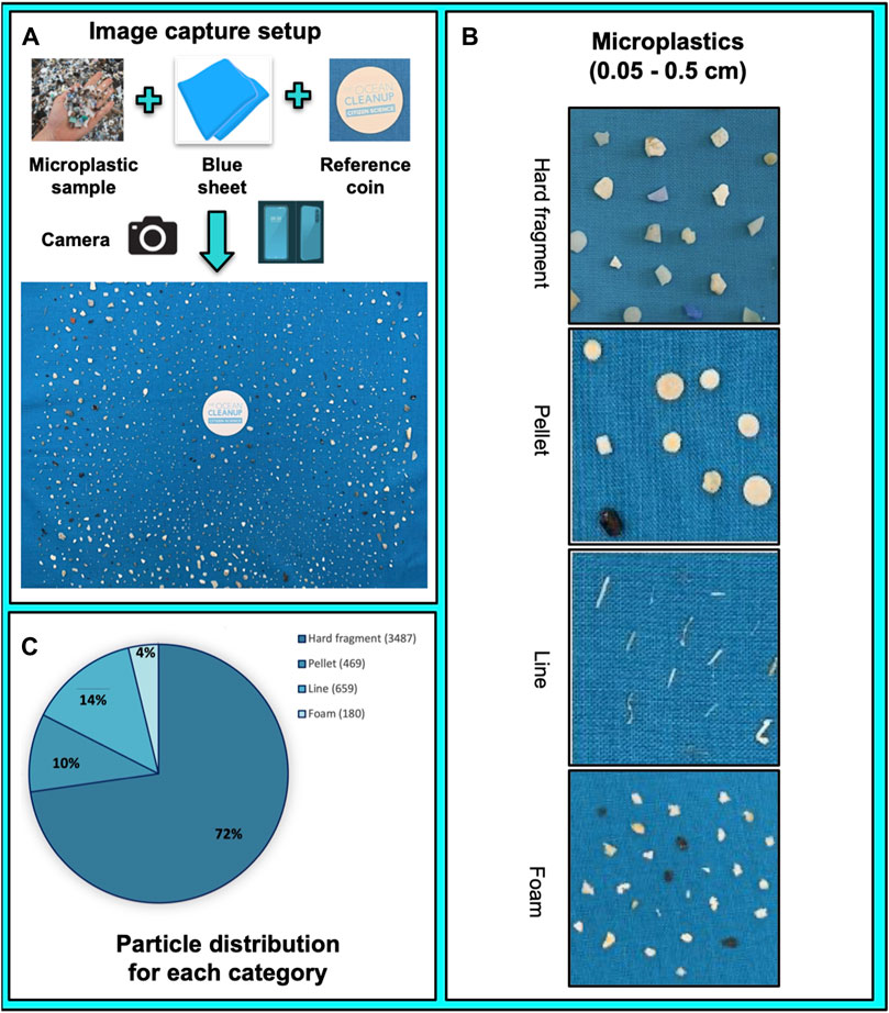
Figure 1. Image prototypes, imagery setup and particle distribution used for the training of the microplastic model with particles ranging from 0.05 to 0.5 cm. (A). Image capture setup demonstrated in chronological order with the final result being the capture of the image. (B). Typical images of the particles are classified into the four categories recognised by the segmentation model: hard fragment, pellet, line, and foam. (C). Particle distribution for each of the categories used by the classifier.

Figure 2

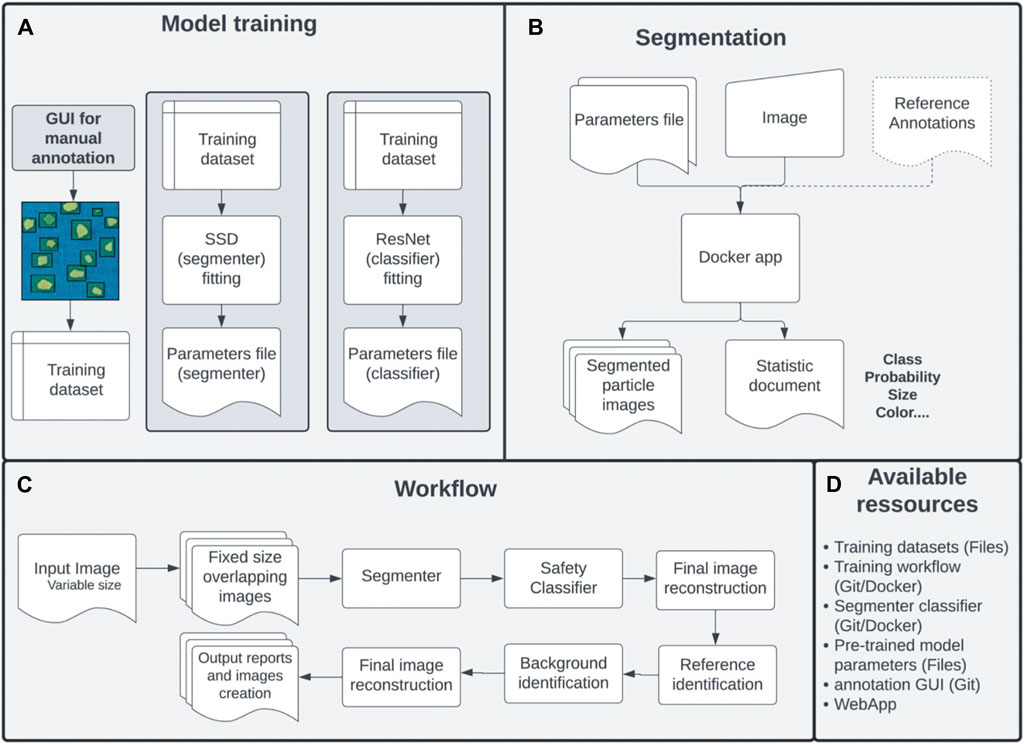
Figure 2. Analytical workflow. (A) A new image is first annotated with a graphical user that allows the storage of the particle type and location within the image. A dataset is then used to train an SSD and a ResNet neural network for segmentation and classification, respectively. (B) A new image is segmented by the workflow using the trained parameters file, which will output a segmented image with individual particle images together with the output TSV file containing the different metrics for each particle. Reference labels for images can optionally be used as input to compare expected versus inferred labels. (C). The segmentation workflow divides the input into multiple overlapped images of fixed size that are segmented. These particles are annotated and the final segmentation is obtained by merging and resolving the annotations for all of the sub-images. A background detection analytical procedure is applied to identify the inferred background of each particle. Different metrics (colors, size, surface area) are inferred for each particle. (D). The workflow is available via a git package docker image or directly through the web portal. The entire dataset with annotation is freely available.

Fine-tuning of the sensitivity and specificity of the segmenter

The sensitivity and the specificity of the segmenter can be fine-tuned with the cutoff parameter which can be seen as a confidence score (default: cutoff = 0.45 with 0 < cutoff <1), of the segmenter to correctly identify a particle within the image. Conversely, training the segmenter with more epochs or a larger, more diverse dataset results in higher overall scores. Essentially, this leads to models with greater confidence in particle identification, enhancing performance, especially in the recognition of low-resolution particles.

Output results and parameters

Each identified particle is labeled in the results file and in an additional output image with a specific particle label allowing to target subsets of particles for further analysis such as Raman spectroscopy or Fourier-transform infrared spectroscopy analysis for polymer identification. The outputted features and coordinates are generated into two TSV files for each individual image processed. The outputted features: ref_color, avg_color, min_length_rectangle, max_length_rectangle, surface, perimeter, min_axis, max_axis, eccentricity, orientation, max_feret_diameter, sum_feret_diameter, class, nb_pixels, nb_pixels_width, nb_pixels_height, equivalent_diameter, are described in Table 1. Amongst these parameters, surface, perimeter, eccentricity, orientation, feret_diameter, and equivalent_diameter are inferred from the Sciki-Image measure class.

Table 1

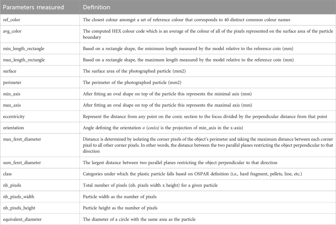
Table 1. List of parameters and their definitions outputted by the computer vision segmentation model after conducting the image analysis.

Performances evaluation

Two strategies were used to evaluate the performance of the classifier and the segmenter. Firstly, we processed validation images through the workflow and compared the expected versus the inferred labels. For doing so, we used the real environmental samples from four stations (see above), took images of them, and used these images as validation datasets that were manually annotated and counted with two methods. We first annotated the images by drawing squares around particles and visually determining their label. In addition, we manually counted the particles and determined their labels directly from the samples. These steps were performed by two different analysts. The particles were manually shuffled to take four additional images for each sample. A comparison between the inferred annotation using the model versus the manual annotations by the user was then conducted. When segmenting an image, our workflow can optionally include reference labels with which the particles inferred from the image are compared.

Secondly, we directly measured the accuracy scores of the labels inferred when training the classifier with a test set where we compared the inferred with the manual counts. We built our validation dataset by collecting plastic particles from four samples and for each sample, we took five different pictures (one image sorted and four manual shuffling) with different particle displays (see above). Having multiple images per sample allowed us to compute a variance for each sample and particle type. We compared the total particle count for each category obtained for each sample with both the manual count obtained from the image and the experimental samples. This was done to estimate the variance between samples but also within samples. When using validation images, the workflow annotates a given particle with the classifier only if the inferred probability is higher than a user-defined threshold (0.60 by default), otherwise the generic annotation “particle” is used. We considered all generic particles as hard fragments since it is the most generic and diverse class and inferred the particle count for each class, sample and image, allowing us to compute the means and variances. These counts were compared to the manual counts obtained directly from the image. Also, for each sample, one of the images was manually segmented. We intersected the manual with the inferred segmentation (see above) and measured how many intersections were found for each sample. Also, the particles were directly counted experimentally when sorting the samples with the manual counts from the image and the experiment performed by two different analysts. To compute the accuracy scores of the classifier, we only used 70% of the dataset for training the classifier and used the remaining 30% as test sets. For each category, we computed the $Precision=\frac{TP}{TP+FP}$, $Recall=\frac{TP}{TP+FN}$, and the $f{1}_{score}=2\frac{Precision.Recall}{Precision+Recall}$ with TP, FP, TN, FP the number of true and false positives and true and false negatives, respectively.

Code availability

The source code and documentation for the computer vision segmentation model framework is free for non-commercial use under Apache 2.0 license. The algorithm for the particle detection can be found at: https://gitlab.com/Grouumf/particle_detect and the web interface to manually annotate a new image can be found at: https://gitlab.com/Grouumf/toc_plastic. The workflow is written in Python3 and tested under Linux, OSX, and Windows. The package contains instructions for installation and usage and the different requirements. Also, a docker image containing all the dependencies installed is also freely available at: docker.io/opoirion/particle_detect.

Availability of data and materials

The full dataset (image and manual annotation) used for training the model is available as Figshare datasets.

Web interface and online portal

A web interface (https://research-segmentation.toc.yt) free to use is now available online per request and allows users to upload their images processed and their respective data available as a TSV file.

Results

Segmentation workflow

A procedure for efficiently quantifying and describing plastic particles within a sample, employing a robust and straightforward method was established. Overall, the model was trained on 68 images divided into 948 overlapping frames, gathering 4,795 particles in total, and used two categories: “reference” or “particle” (Figure 2B). To elaborate, each particle is first segmented (Figure 2C) as a generic “particle” thereby reducing the false negative detection rate of the segmenter if all categories were used directly (Supplementary Figure S1). Subsequently, a classifier trained on the 4,795 particles, labels each segmented particle into four categories: “hard”, “pellet”, “line”, or “foam”. Finally, the annotated particles are characterized with multiple image transformations to extract multiple geometrical properties such as surface area, dimensions, and colors (see Methods for more details). If a reference coin is present, the workflow will automatically infer the absolute size of a pixel to convert the relative sizes and surfaces of the particles inferred. It is accessible as a Git package or Docker image, accompanied by thorough documentation at https://gitlab.com/Grouumf/particle_detect for the main pipeline. A user-friendly web interface, outlined below, has also been created.

Model validation

For assessing the accuracy and the performance of the model, the output of images processed by the model was compared to particles that were counted manually using the same samples. The particles in the selected environmental samples (Supplementary Figure S1) corresponded to the four commonly found categories for microplastics (hard fragment, pellet, line, and foam). Examples for each category are shown in Figure 1B. Reflecting the real distribution, unequal numbers of particles were used for each category but a minimum of at least 200 particles was used for each category. Hard fragments predominated, constituting 72% of the total particles. Lines, pellets, and foams made up smaller fractions, with 14%, 10%, and 4%, respectively (Figure 1C). These two approaches (model output vs manual count) indicated both methods to be similar with a small variance and a count varying between 298 and 822 for the four different microplastic categories provided by the model and used for manual annotation.

Performances and limitations of the models

To assess the performance of the workflow we used the real environmental samples from the four stations (see above), took images of them, and used these images as validation datasets (Figure 3). For each sample, the overall accuracy of the segmenter was evaluated by comparing the number of matches/mismatches between the inferred and annotated image labels (Figures 3B, C). Overall, the segmenter was able to identify more than 96% of the particles for the four samples selected and was fast with an average processing time of less than 25 s per image on a regular laptop. However, as the particles become smaller the performance of the model decreases. Indeed, smaller particles have higher chances of being either missed or being a false positive, with all the missing annotated particles (1%). The performance of the segmenter is not solely driven by the size of the particles but even more so by the number of pixels per frame, highlighting the importance of taking high-resolution images for particle count. The optimum number of pixels is 45–65 pixels per frame. In some cases, and this varies when adjusting the sensitivity of the image, the model can either miss particles or annotate particles that were not seen by the operator and are considered as noise. The latter might be due to patterns from the blue sheets or noise from the image that results in the overestimation of the number of particles.

Figure 3

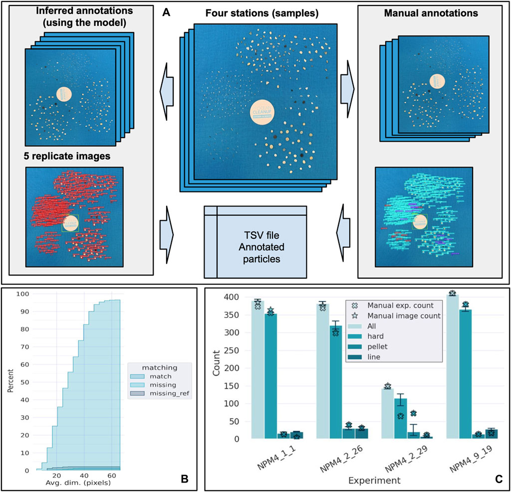
Figure 3. Segmenter performance based on the selection of four oceanographic stations where samples of microplastics were collected using a manta trawl that filtered surface seawater in the North Pacific Garbage Patch during the North Pacific Mission 4 led by The Ocean Cleanup in 2022. (A). For each of the four stations, the particles were shuffled four times with mixed particles dispersed across the sheet, one image was also taken where all of the particles were categorized manually. These five resulting images were used as replicates for the inferred annotation analysis (left) and the manual annotation analysis (right). The inferred annotation using the model provides an output image with the particles segmented. The red box represents a particle captured by the model and numbered (Figure 3A left). The manual annotation that corresponds to the drawing of a rectangle around each particle manually provides an output image with the particles segmented with three distinct colors (Figure 3A right). Cyan represents a match between the inferred and the manual annotations, red represents the missing annotated particles, and purple represents unannotated particles, meaning these were captured by the model but not annotated manually. (B). The comparison between the manual experimental count (hand-counted), the manual image count (annotation), and the inferred count (model) using visual images. Results are shown for all of the particles (light cyan) and the three separate categories (hard fragment, pellets, and lines). The cross corresponds to the manual count referred to as the manual experimental count and the star corresponds to the manual image count that was conducted by an independent operator. The bars and the error bars represent the mean for the data generated by the model estimated using the five replicates per station, respectively. The stars represent the manual counts. (C). The cumulative distribution of the matching particles between the annotated and inferred label, the missing particles from the reference (false positive), and the missing particles from the classifier (false negative) as a function of the pixel size.

False positives refer to instances where the segmenter annotates particles that do not actually exist, including noise, reflections, disturbances, or the sheet matrix. However, a fraction of these particles was simply not manually annotated due to their small size rendering them barely visible to the human eye (Supplementary Figure S2). The flexibility of the workflow allows for the adjustment of sensitivity and specificity by fine-tuning the detection thresholds of the segmenter model (see below). Additional analyses were also conducted to assess the effect of the dimensions of the pixel (image resolution) related to the percent of successes, highlighting an overall 97% of successful matches (Figures 3B, C). Moreover, all missing reference particles and false positive particles wrongfully detected by the workflow were less than 40 pixels wide. Supplementary Figure S3 is a different way of visualizing the effect of the pixel dimensions versus the performance of the model (100% being perfect) where on average in proportion, false positive and false negative occur for smaller particles which are harder to detect as demonstrated above. Hence, data demonstrates that as we decrease the pixel dimension the results are further away from 100% where an increase in false positives and false negatives are seen for smaller pixel sizes (Supplementary Figure S3). Furthermore, amongst the particles annotated only by the segmenter (putative false positive), we found that a significant fraction were small particles missed by the analyst (Supplementary Figure S2). Others seem to be either ambiguous or originated because of patterns from the background misleading the segmenter (Supplementary Figure S2).

Classification performance

To estimate the accuracy of labels inferred, we compared the inferred and the manual counts of the four selected samples and computed a variance for each sample and particle type. and observed overall a very good agreement between the observed and expected counts (Figure 3B). The average observed error was less than 2% ( ± 1%) for identifying the particles, however, a larger error was observed for identifying the correct labels for pellets, hard fragments, and lines which are explained by the visual similarities of some particles of a given class with another (Figure 4). Indeed, it was virtually impossible to manually correct some of the mislabeled particles based only on visual attributes (Figure 4A). It is worth noting that the observed error remains in most cases small. For example, three out of the four samples have an error of less than 5% for the hard fragments, while the fourth sample (NPM4_2_29) had an error of 25%. This could be explained by the lower number of annotated hard fragments (65) and their similarities with the pellets (Figure 4A).

Figure 4

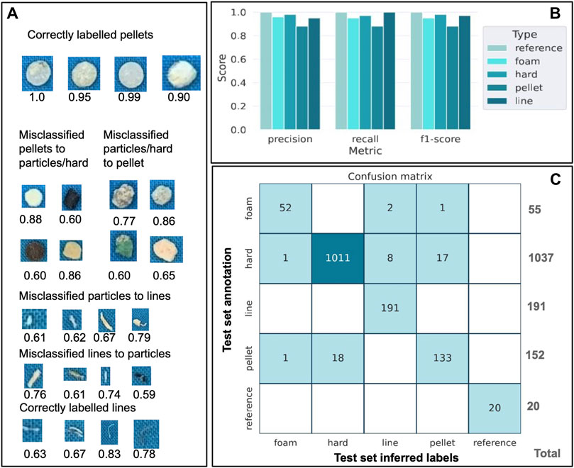
Figure 4. Classifier performance based on the test dataset representing 30% of the full dataset (30% of 4,795 particles). (A). Examples of mis-annotated particles and the resemblance between the different categories for these mismatches. The number below each annotated particle represents the f1-score. (B). The score for the precision, the recall, and the f1-score are shown for the reference (score = 1.0) and the different categories of the test data set (hard fragment, pellet, line. and foam particles). (C). Confusion matrix displaying the match between the test set inferred labels and the test set annotation for the reference and the different categories of the test data set (hard fragment, pellet, line, and foam particles). Note that the results should be read horizontally (i.e., the classifier shows most difficulties in distinguishing pellets from hard fragments with 18 misclassified particles for the pellets.

Precision and recall are convenient metrics to reflect the true positive rates amongst labeled and unlabeled particles of a given class while the f1-score reflects the overall accuracy. We then assessed the classification performance by randomly creating a test dataset containing 30% (1,439 particles) of the particles and trained our classifier on the remaining 70% (3,556 particles). From the labels inferred from the test dataset, we obtained high precision, recall, and f1-score for all classes, with the highest scores obtained for the reference (f1-score = 1.0), followed by the hard fragments (f1-score = 0.98) and the lowest obtained for the pellets (f1-score = 0.88) (Figure 4B), with an average weighted f1-score of 0.97. The most significant mislabeling occurs with pellets being identified as hard fragments, or vice versa. This highlights the classifier’s challenges in distinguishing between pellets and hard fragments (Figure 4C), attributed to the striking similarity in shape, size, and colors of both categories. Small lines are also particularly hard to distinguish since their shape, size, and morphology overlap with other small-type particles (Figure 4C). Overall, larger and very distinct particles such as long lines and hard fragments with sharp edges are easily identifiable and thus correctly labeled.

Workflow calibration

The efficiency of our workflow is intricately linked to the quality and resolution of the analyzed images. Thus, it is crucial to possess the capability to fine-tune sensitivity and specificity, tailored to the specifics of each experimental setup. To achieve this objective, our workflow provides the flexibility to incorporate external labels and annotations, serving as benchmarks for comparison with the particles and annotations inferred by the model (see Methods). Additionally, we have developed an intuitive Graphical User Interface (GUI) to facilitate the annotation of new images (see Methods). By leveraging annotated reference images, the sensitivity and specificity of the segmentation can be precisely adjusted through a customizable cutoff hyperparameter (see Methods). Lowering this cutoff enhances the workflow’s sensitivity by identifying lower-resolution particles. However, it also leads to an increase in false positives—annotated particles that do not correspond to actual particles. Likewise, the classifier’s sensitivity and specificity can be configured using a distinct cutoff. Increasing this cutoff will lower the frequency of misclassified particles, albeit at the cost of a higher occurrence of particles that will retain the generic “particle” label by not meeting the threshold criteria.

Training and processing time

Thanks to the use of a relatively simple model architecture (SSD and ResNet56, see Methods), training a new segmentation or classification model can be performed with CPUs of a standard laptop in a reasonable time. The time required to train one epoch was measured, which corresponds to using all the training samples one time, using a standard laptop CPU (Intel i7 1.8 GHz). We measured 900 s for 1,000 frames of 600 × 600 pixels for the segmenter (Figure 5A) and of 31 s for 4,000 particles of 48 × 48 pixels per frame for the classifier (Figure 5B). We also found a linear relationship in the processing time with a maximum of 35 s and an increasing number of particles with dimensions (frame width, Figure 5C). These results indicate that these models can be directly built on conventional computers. In practice, we trained our models on faster CPUs using 600 and 1,200 epochs for a total training time of two and six hours for the classifier and the segmenter respectively.

Figure 5

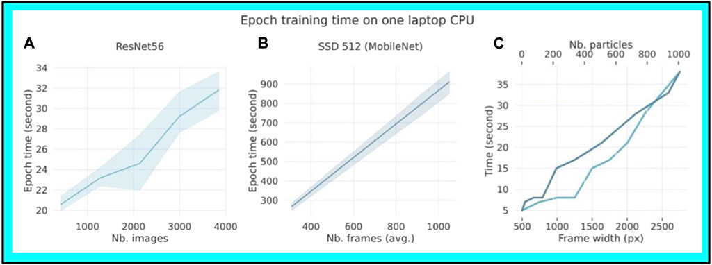
Figure 5. Speed efficiency and training time per Epoch using a conventional Intel i7 1.8 GHz Laptop CPU. (A) A given number of particles processed by the segmenter SSD 512 against the epoch time (sec) using a conventional CPU laptop. The input images were 600 × 600 pixels per frame. (B) A given number of particles processed by the classifier ResNet56 against the epoch time (sec). The input images were 48 × 48 pixels per frame. The light cyan represents the variability around the mean for each data point. (C). The frame width and the number of particles against the processing time (sec).

Freely accessible web interface

A freely accessible web interface has been developed for the seamless upload and processing of images. The interface generates a TSV file containing all measured parameters. The image processing involves both segmentation and classification of particles, with flexibility in selecting either the micro or meso model (briefly described in the Supplementary Material). This graphical interface is available at no cost and can be accessed upon request via the following web address: https://research-segmentation.toc.yt/. The website offers a concise, clean, and efficient user experience. Upon initial use, the user creates an account, enters image-related information, and selects parameters like the size of the reference coin (default value is 37 mm) and sensitivity, which can be fine-tuned later through the cut-off setting (Figure 6). After completing these steps, the image can be uploaded. In the second phase, once all required details are entered, the job is submitted, and the image undergoes processing. The process is swift, and the results, along with the processed image, are organized in a dedicated section of the app. Here, users can easily visualize and download all results. Multiple results can be conveniently assembled and accessed in the future under the user’s identification. The portal offers live updates for newer models, allowing users to choose the most up-to-date version for their work. This flexibility is particularly valuable for maintaining consistency in processing samples over time series, while also providing opportunities for optimizing methods and improving results.

Figure 6

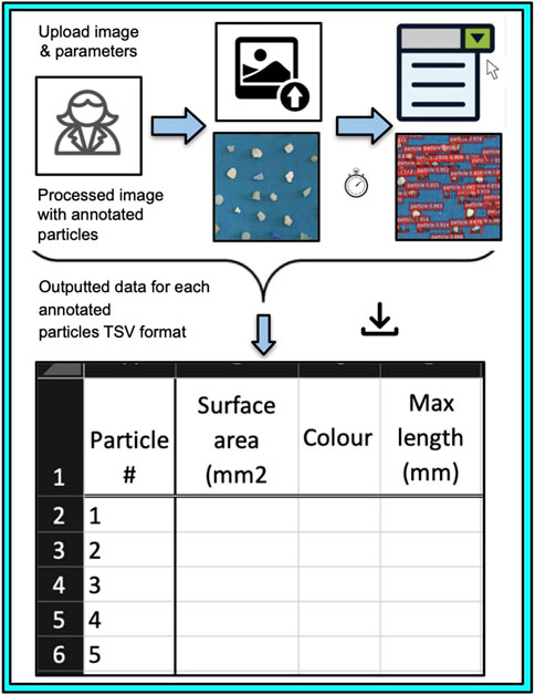
Figure 6. Segmentation model accessibility and the processing of a new image using the graphical web interface. A Scheme of the graphical web interface that is readily available and free of charge for users and allows the generation of the data after the processing of the image and available as a TSV file.

Discussion

Estimation of microplastic concentrations in the environment is a challenging task due to the large varieties of terrestrial and oceanic environments, the wide range of plastic sources, and the variability in the shapes, sizes, and types of microplastic particles. To streamline and standardize essential steps in the process, we advocate for a dual-pronged standardized methodology. The first step involves capturing images of microplastic samples through a straightforward experimental procedure, while the second step focuses on processing these images using computer vision approaches in the modeling phase. In summary, this workflow establishes a robust method for the characterization of microplastics and we believe it offers significant advantages described below.

Reporting plastic particle size is crucial as it plays a critical role in understanding size distributions, predicting the eventual fate of plastic particles in various environments, and for their impact and risk analysis in these environments (Koelmans et al., 2022; Schnepf, 2023). However, variations in reported plastic particle sizes are common which can often be attributed to the different methods of measurements. To date, the two most widely used methods to measure plastic particle size or size distribution are based on visual observation with manual measurements through the use of rulers or post-processing using a numerical model with a size reference and sieving (Reinhardt, 2021; Huang et al., 2023). Microscopic techniques such as electron scanning microscopy (Hidalgo-Ruz et al., 2012; Shim et al., 2017) and laser diffraction particle size analysis (Huang et al., 2023) are also two techniques that are gaining popularity in reporting plastic particle sizes (Shim et al., 2017). Each method will produce different results due to the nature of the distinctive measurement techniques. For example, visual measurements usually report the maximum length or diameter of the particle, whereas in microscopy it is common to report the Feret’s diameter, which is the distance between two tangents on opposite sides of a particle and parallel to a fixed dimension (Reinhardt, 2021).

Overall, our model presents important benefits with regard to manual annotation. First, it greatly improves the annotation speed, diminishes the complexity of the preparation and thus cost-effectiveness. Secondly, multiple morphological characteristics difficult to measure manually such as the surface area, the diameter, or the color, are inferred. It is also very valuable to be able to view the particle sizes as a continuous dataset instead of in discrete size fractions binned in sizes of 0.05–0.15 cm, 0.15–0.5 cm, etc. Other advantages are the replicability of the method, the possibility of making changes to the script and adapting it to specific datasets, and the ease of using the model by different organizations and communities. With regards to speed efficiency, our workflow can process a high-resolution image containing more than 800 particles in less than 30 s. The speed difference with manual counting will be even more magnified when using larger images with high numbers of particles. Another important advantage of our workflow is the ability to mitigate sampling bias through impartial particle annotations. This stands in contrast to human annotations, which may be prone to variations, especially when multiple annotators interpret the annotation guidelines differently.

In general, comparing studies becomes challenging because of the diverse data collection methods employed. Furthermore, as sample sizes increase and particle sizes decrease, conventional visual techniques become increasingly labor-intensive and intricate. Our segmentation workflow on the other hand, provides consistent measurements with the possibility of adding more parameters, identically regardless of the data collector and environmental compartments where the particles were sampled. The workflow not only offers greater consistency and efficiency in comparison to the manual techniques employed today but also mitigates the potential for human error. Furthermore, the data generated after the processing of the images provide parameters difficult or time-consuming to measure with manual characterization, such as the surface area of the particle, the perimeter, and the eccentricity (“roundness”). These additional parameters open up new possibilities for quantitative comparison within the realm of plastic pollution in various environmental compartments.

Our workflow also grants users to customize the script and tailor the algorithm to their specific datasets, enabling, for example, the inclusion or exclusion of additional categories, or changing the sensitivity detection thresholds. Consequently, our method can be seamlessly adapted to diverse environmental conditions, facilitating the estimation of plastic concentrations in water bodies, along shorelines, and even in sediments. This uniform approach enables the monitoring of different environments using the same method, capturing the evolution of microplastic concentrations over time. Finally, our workflow is available through a user-friendly graphical interface enhancing ease of use for a broad audience, directly segmenting an input image and storing the results online. This accessibility is particularly beneficial for diverse communities engaged in plastic pollution research, ensuring that the method is readily available and easily utilized by different stakeholders.

Currently, an experimental model exists for meso (0.5–5 cm) and macro (>5 cm) plastic objects. However, insufficient annotated data hampers its performance. Ongoing efforts involve collecting more particles in these size ranges to enhance the model. Accessible online, the model and the datasets support individual users and benefiting diverse researchers and citizen scientists in the plastic pollution community. Furthermore, upcoming developments could lead to the availability of new models trained on additional particle classes or more extensive datasets.

While the model presents several advantages, it also has notable limitations. Visual recognition alone does not allow users to assess the three dimensions of particles. This limitation affects distinguishing between foam and pellets versus hard fragments, where touch and three-dimensional evaluation are beneficial. By touching these two different types of items, the user can evaluate the particle being a foam by feeling the texture and can also identify a pellet better by its 3D-rounded shape that can be hard to detect from an image.

In summary, while the segmenter achieves high accuracy in particle counting, the classifier’s performance is lower, particularly for categories with high variability, such as pellets and smaller foam particles. Increasing further the number of particles in the training dataset is expected to improve performance for these categories. The hard fragment category, with its diverse shapes and sizes, dominates the training dataset, leading to a higher annotation of hard fragment particles by the model. This aligns with environmental sample realities, as demonstrated by Egger et al. (2020) in the NPGP, where hard fragments prevail. User-dependent qualitative data could introduce variability, but the model ensures repeatability and standardization in microplastic categorization. Understanding the limitations is crucial for interpreting the data appropriately for its intended use but we believe this methodology will significantly improve data quality.

Data availability statement

The raw data supporting the conclusion of this article will be made available by the authors, without undue reservation.

Author contributions

S-JR: Conceptualization, Data curation, Investigation, Methodology, Project administration, Resources, Supervision, Validation, Visualization, Writing–original draft, Writing–review and editing. HW: Conceptualization, Data curation, Investigation, Writing–review and editing. AD: Data curation, Investigation, Resources, Validation, Writing–review and editing. LL: Conceptualization, Funding acquisition, Investigation, Supervision, Writing–review and editing. OP: Conceptualization, Data curation, Formal Analysis, Investigation, Methodology, Resources, Software, Supervision, Validation, Visualization, Writing–original draft, Writing–review and editing.

Funding

The author(s) declare financial support was received for the research, authorship, and/or publication of this article. This work was funded by the donors of The Ocean Cleanup Foundation.

Acknowledgments

The authors are grateful to the donors of The Ocean Cleanup who sponsored this study. The authors are also grateful to the help of Maarten van Berkel, Chiel Peters, and Kiki van Rongen for their help and support for the setup of the web interface. AD has received funding from the European Union’s Horizon Europe research and innovation program under the Marie Sklodowska-Curie grant agreement No 101061749. AD has a project endorsed as “No 93.2. PlaSTic On beaches: 3D-distRibution and weathering” as part of the UN Decade of Ocean Science for Sustainable Development 2021-2030, and is attached to the Ocean Decade Programme “15. Early Career Ocean Professionals (ECOPs).

Conflict of interest

The authors declare that the research was conducted in the absence of any commercial or financial relationships that could be construed as a potential conflict of interest.

Publisher’s note

All claims expressed in this article are solely those of the authors and do not necessarily represent those of their affiliated organizations, or those of the publisher, the editors and the reviewers. Any product that may be evaluated in this article, or claim that may be made by its manufacturer, is not guaranteed or endorsed by the publisher.

Supplementary material

The Supplementary Material for this article can be found online at: https://www.frontiersin.org/articles/10.3389/fenvs.2024.1386292/full#supplementary-material

References

Billard, G., and Boucher, J. (2019). The challenges of measuring plastic pollution. F. Actions Sci. Rep. 2019, 68–75.

Google Scholar

Chen, T., Li, M., Li, Y., Lin, M., Wang, N., Wang, M., et al. (2015). MXNet: a flexible and efficient machine learning library for heterogeneous distributed systems. ArXiv 1–6. doi:10.48550/arXiv.1512.01274

CrossRef Full Text | Google Scholar

Critchell, K., Bauer-Civiello, A., Benham, C., Berry, K., Eagle, L., Hamann, M., et al. (2019). Plastic pollution in the coastal environment: current challenges and future solutions. Coasts Estuaries Future. Elsevier Inc., 595–609. doi:10.1016/B978-0-12-814003-1.00034-4

CrossRef Full Text | Google Scholar

Critchell, K., Grech, A., Schlaefer, J., Andutta, F. P., Lambrechts, J., Wolanski, E., et al. (2015). Modelling the fate of marine debris along a complex shoreline: lessons from the Great Barrier Reef. Estuar. Coast. Shelf Sci. 167, 414–426. doi:10.1016/j.ecss.2015.10.018

CrossRef Full Text | Google Scholar

Critchell, K., and Lambrechts, J. (2016). Modelling accumulation of marine plastics in the coastal zone; what are the dominant physical processes? Estuar. Coast. Shelf Sci. 171, 111–122. doi:10.1016/j.ecss.2016.01.036

CrossRef Full Text | Google Scholar

Eriksen, M., Lebreton, L. C. M., Carson, H. S., Thiel, M., Moore, C. J., Borerro, J. C., et al. (2014). Plastic pollution in the world’s oceans: more than 5 trillion plastic pieces weighing over 250,000 tons afloat at sea. PLoS One 9, e111913–e111915. doi:10.1371/journal.pone.0111913

PubMed Abstract | CrossRef Full Text | Google Scholar

Europe, P. (2021). Plastics Europe association of plastics manufacturers plastics—the facts 2021 an analysis of European plastics production. Demand Waste Data.

Google Scholar

GESAMP (2015). Sources, fate and effects of microplastics in the marine environment: a global assessment. Rep. Stud. GESAMP. doi:10.13140/RG.2.1.3803.7925

CrossRef Full Text | Google Scholar

GESAMP (2019). Guidelines for the monitoring and assessment of plastic litter in the ocean. Rep. Stud. GESAMP no 99, 130p.

Google Scholar

González-fernández, D., Cózar, A., Hanke, G., Viejo, J., Morales-caselles, C., Bakiu, R., et al. (2021). Floating macrolitter leaked from Europe into the ocean. Nat. Sustain. 4, 474–483. doi:10.1038/s41893-021-00722-6

CrossRef Full Text | Google Scholar

Guo, J., He, H., He, T., Lausen, L., Li, M., Lin, H., et al. (2020). GluonCV and gluon NLP: deep learning in computer vision and natural language processing. J. Mach. Learn. Res. 21, 1–7.

PubMed Abstract | Google Scholar

Hartmann, N. B., Hüffer, T., Thompson, R. C., Hassellöv, M., Verschoor, A., Daugaard, A. E., et al. (2019). Are we speaking the same language? Recommendations for a definition and categorization framework for plastic debris. Environ. Sci. Technol. 53, 1039–1047. doi:10.1021/acs.est.8b05297

PubMed Abstract | CrossRef Full Text | Google Scholar

Haward, M. (2018). Plastic pollution of the world’s seas and oceans as a contemporary challenge in ocean governance. Nat. Commun. 9, 667–711. doi:10.1038/s41467-018-03104-3

PubMed Abstract | CrossRef Full Text | Google Scholar

He, K., Zhang, X., Ren, S., and Sun, J. (2016). Deep residual learning for image recognition. Proc. IEEE Comput. Soc. Conf. Comput. Vis. Pattern Recognit. 2016-Decem, 770–778. doi:10.1109/CVPR.2016.90

CrossRef Full Text | Google Scholar

Hidalgo-Ruz, V., Gutow, L., Thompson, R. C., and Thiel, M. (2012). Microplastics in the marine environment: a review of the methods used for identification and quantification. Environ. Sci. Technol. 46, 3060–3075. doi:10.1021/es2031505

PubMed Abstract | CrossRef Full Text | Google Scholar

Huang, Z., Hu, B., and Wang, H. (2023). Analytical methods for microplastics in the environment: a review. Environ. Chem. Lett. 21, 383–401. doi:10.1007/s10311-022-01525-7

PubMed Abstract | CrossRef Full Text | Google Scholar

Isobe, A., and Iwasaki, S. (2022). The fate of missing ocean plastics: are they just a marine environmental problem? Sci. Total Environ. 825, 153935. doi:10.1016/j.scitotenv.2022.153935

PubMed Abstract | CrossRef Full Text | Google Scholar

Kaandorp, M. L. A., Lobelle, D., Kehl, C., Dijkstra, H. A., and Van Sebille, E. (2023). Global mass of buoyant marine plastics dominated by large long-lived debris. Nat. Geosci. 16, 689–694. doi:10.1038/s41561-023-01216-0

CrossRef Full Text | Google Scholar

Koelmans, A. A., Redondo-Hasselerharm, P. E., Nor, N. H. M., de Ruijter, V. N., Mintenig, S. M., and Kooi, M. (2022). Risk assessment of microplastic particles. Nat. Rev. Mater. 7, 138–152. doi:10.1038/s41578-021-00411-y

CrossRef Full Text | Google Scholar

Kornilov, A. S., and Safonov, I. V. (2018). An overview of watershed algorithm implementations in open source libraries. J. Imaging 4, 123. doi:10.3390/jimaging4100123

CrossRef Full Text | Google Scholar

Law, K. L., Morét-Ferguson, S. E., Goodwin, D. S., Zettler, E. R., Deforce, E., Kukulka, T., et al. (2014). Distribution of surface plastic debris in the eastern Pacific Ocean from an 11-year data set. Environ. Sci. Technol. 48, 4732–4738. doi:10.1021/es4053076

PubMed Abstract | CrossRef Full Text | Google Scholar

Lebreton, L., Egger, M., and Slat, B. (2019). A global mass budget for positively buoyant macroplastic debris in the ocean. Sci. Rep. 10, 12922. doi:10.1038/s41598-019-49413-5

PubMed Abstract | CrossRef Full Text | Google Scholar

Lebreton, L., Slat, B., Ferrari, F., Sainte-Rose, B., Aitken, J., Marthouse, R., et al. (2018). Evidence that the great pacific garbage Patch is rapidly accumulating plastic. Sci. Rep. 8, 4666. doi:10.1038/s41598-018-22939-w

PubMed Abstract | CrossRef Full Text | Google Scholar

Liu, W., Anguelov, D., Erhan, D., Szegedy, C., Reed, S., Fu, C.-Y., et al. (2016). SSD: Single Shot MultiBox detector. ECCV 1, 398–413. doi:10.1007/978-3-319-46448-0

CrossRef Full Text | Google Scholar

Lorenzo-Navarro, J., Castrillón-Santana, M., Sánchez-Nielsen, E., Zarco, B., Herrera, A., Martínez, I., et al. (2021). Deep learning approach for automatic microplastics counting and classification. Sci. Total Environ. 765, 142728. doi:10.1016/j.scitotenv.2020.142728

PubMed Abstract | CrossRef Full Text | Google Scholar

Lorenzo-Navarro, J., Castrillon-Santana, M., Santesarti, E., De Marsico, M., Martinez, I., Raymond, E., et al. (2020). SMACC: a system for microplastics automatic counting and classification. IEEE Access 8, 25249–25261. doi:10.1109/ACCESS.2020.2970498

CrossRef Full Text | Google Scholar

Mukhanov, V. S., Litvinyuk, D. A., Sakhon, E. G., Bagaev, A. V., Veerasingam, S., and Venkatachalapathy, R. (2019). A new method for analyzing microplastic particle size distribution in marine environmental samples. Ecol. Montenegrina 23, 77–86. doi:10.37828/em.2019.23.10

CrossRef Full Text | Google Scholar

Provencher, J. F., Covernton, G. A., Moore, R. C., Horn, D. A., Conkle, J. L., and Lusher, A. L. (2020a). Proceed with caution: the need to raise the publication bar for microplastics research. Sci. Total Environ. 748, 141426. doi:10.1016/j.scitotenv.2020.141426

PubMed Abstract | CrossRef Full Text | Google Scholar

Razzell, J., Gabrielle, H., Jennifer, H., Rea, E., Komyakova, V., and Bond, A. L. (2023). Quantitative photography for rapid, reliable measurement of marine macro-plastic pollution. Methods Ecol. Evol. 2023, 1–17. doi:10.1111/2041-210X.14267

CrossRef Full Text | Google Scholar

Reinhardt, I. (2021) Modelling of features of microplastics in soil. USA: Univ. Stuuttgart.

Google Scholar

Ryan, P. G., Weideman, E. A., Perold, V., and Moloney, C. L. (2020). Toward balancing the budget: surface macro-plastics dominate the mass of particulate pollution stranded on beaches. Front. Mar. Sci. 7, 1–14. doi:10.3389/fmars.2020.575395

PubMed Abstract | CrossRef Full Text | Google Scholar

Schnepf, U. (2023). Realistic risk assessment of soil microplastics is hampered by a lack of eligible data on particle characteristics: a call for higher reporting standards. Environ. Sci. Technol. 57, 3–4. doi:10.1021/acs.est.2c08151

PubMed Abstract | CrossRef Full Text | Google Scholar

Shim, W. J., Hong, S. H., and Eo, S. E. (2017). Identification methods in microplastic analysis: a review. Anal. Methods 9, 1384–1391. doi:10.1039/c6ay02558g

CrossRef Full Text | Google Scholar

Thompson, R. C., Moore, C. J., Saal, F. S. V., and Swan, S. H. (2009). Plastics, the environment and human health: current consensus and future trends. Philos. Trans. R. Soc. B Biol. Sci. 364, 2153–2166. doi:10.1098/rstb.2009.0053

PubMed Abstract | CrossRef Full Text | Google Scholar

Walker, T. R., and Fequet, L. (2023). Current trends of unsustainable plastic production and micro(nano)plastic pollution. Trac. - Trends Anal. Chem. 160, 116984. doi:10.1016/j.trac.2023.116984

CrossRef Full Text | Google Scholar

Waller, C. L., Griffiths, H. J., Waluda, C. M., Thorpe, S. E., Loaiza, I., Moreno, B., et al. (2017). Microplastics in the Antarctic marine system: an emerging area of research. Sci. Total Environ. 598, 220–227. doi:10.1016/j.scitotenv.2017.03.283

PubMed Abstract | CrossRef Full Text | Google Scholar

Weiss, L., Ludwig, W., Heussner, S., Canals, M., Ghiglione, J. F., Estournel, C., et al. (2021). The missing ocean plastic sink: gone with the rivers. Sci. (80-. ) 373, 107–111. doi:10.1126/science.abe0290

CrossRef Full Text | Google Scholar

Zhang, Y., Zhang, D., and Zhang, Z. (2023). A critical review on artificial intelligence—based microplastics imaging technology: recent advances, hot-spots and challenges. Int. J. Environ. Res. Public Health 20, 1150. doi:10.3390/ijerph20021150

PubMed Abstract | CrossRef Full Text | Google Scholar