Flexibility evaluation of psammophytes using Young’s modulus based on 3D numerical simulation

Flexible psammophytes play an important role in controlling soil wind erosion and desertification, owing to their characteristics. Although flexibility of psammophytes has been considered in previous studies, the interaction between flexible psammophytes and the surrounding airflow field still remained unclear. In this study, we used the Young’s modulus to describe plant flexibility and conducted a 3D computational fluid dynamics simulation using a standard k-ε model and a fluid–structure interaction model. Taking Caragana korshinskii (Caragana), a typical psammophyte, as the research object, we constructed 3D geometric models with different diameters to simulate the airflow field around the flexible psammophytes. By comparing with the simulation results of rigid plants and simulation results of flexible plants at different wind speeds, we could verify the rationality of the simulation method. Based on the simulation results, the maximum swing amplitude of the model and the Young’s modulus were found to have a negative correlation, presenting an exponential functional relationship with good fitting. The relationship between the actual Young’s modulus of the plant branches and that of different diameter models in the numerical simulation was also established. This study is expected to improve our basic understanding of the interaction between flexible psammophytes and the surrounding airflow field, and provide some qualitative reference for the numerical simulation of the airflow field around flexible psammophytes.

1 Introduction

Psammophytes are plants that grow in sandy soil environments. Given their adaptability to the growing environment, they typically exhibit a series of ecological characteristics, including wind erosion resistance, sand cutting resistance, burning resistance, and drought resistance. Owing to these characteristics, psammophytes play an important role in controlling soil wind erosion and desertification. The impact of psammophytes on soil protection is complex. Plant coverage, shape, canopy morphology, leaf area, and flexibility have different degrees of impact on soil protection (Tang et al., 2011; Qu et al., 2012). In general, the protective effects of these factors on soil formation are mainly embodied in the pattern variation in the surrounding airflow field and decrease in the wind speed and sand interception by the plant (Qu et al., 2012). Researchers have qualitatively and quantitatively evaluated the effects of coverage (Liu et al., 2021), shape (Liu et al., 2021), canopy morphology (Liu et al., 2018), and leaf area (Zhang et al., 2008) on the shelter benefit and sand intercepting capacity of psammophytes. With the advancement of studies on the mechanism of wind erosion resistance, the flexibility of psammophytes has been found to be an important factor affecting the distribution of the airflow fields around the plants. On one hand, the branches of flexible plants deform and swing under the action of airflow. On the other hand, plants with structural deformation and swinging also disturb the airflow and affect the distribution of the airflow field (Abulaiti et al., 2016). Therefore, plants with different flexibility have varied effects on controlling wind erosion, and it is necessary to quantitatively study the flexibility of psammophytes.

The flexibility of plants was first studied on aquatic plants, and the mechanism of the impact of flexible aquatic plants on water flow was found to be much more complicated than that of the impact of rigid plants (Qu et al., 2012). A previous study analyzed the correlation between plant density and flexibility, and hydraulic resistance, thus pointing out the logarithmic distribution of velocity (Kouwen et al., 1969). Järvelä, (2002) examined the flow resistance of natural grasses, sedges, and willows in a laboratory flume and found the flexibility has an obvious effect on the friction coefficient of water flow. Wu and Jiang, (2008) found that the turbulence intensity of the water flow with rigid plants is much higher than that of the water flow with flexible plants, especially at the plant canopy. To study the flexibility of psammophytes, a literature review indicated that owing to the similarity of the fluid, the concept of aquatic rigid and flexible plants can be applied to the study of wind dynamics (Tang et al., 2011). Furthermore, Qu et al. (2012) pointed out that flexible psammophytes are distributed in desertified areas, have branches with certain toughness, and evidently swing and bend along the wind direction under the action of wind. Furthermore, there is no evident dividing line between flexible and rigid plants.

Currently, the commonly used methods to study flexible psammophytes include field observations (Grant and Nickling, 1998; Leenders et al., 2007; Li et al., 2007; Tang et al., 2011), wind-tunnel experiments (Guan et al., 2003; Walter et al., 2012; Abulaiti et al., 2016; Kang et al., 2019; 2020), and numerical simulations (Mayaud et al., 2016; Fang, 2019; Wu et al., 2022; 2023). Most previous studies on the wind erosion resistance of plants were based on wind-tunnel tests. A field observation and wind-tunnel test on shrub sand piles was conducted to investigate the impact of roughness elements on sand transport efficiency. In a wind-tunnel test, they compared flexible (using fake grass) and rigid (using tufts of stiff wire) roughness elements, and found that using low-flexibility plants will effectively reduce dust emission more than using high-flexibility plants (Abulaiti et al., 2016). Kang et al. (2020) compared the characteristics of surface wind speed profiles of two types of flexible plants based on a wind-tunnel test. The change in the airflow field structure indicates that the flexibility of plant stems and branches is an important factor affecting the sediment resistance of plants. However, it is difficult to simulate plant flexibility in wind tunnels, and model materials are bound to be inconsistent with those of real plants. In addition, many species of psammophytes grow in sandy land, and their morphologies are diverse, which cannot be completely modeled in wind tunnels (Qu et al., 2012).

Compared with conventional wind-tunnel tests, a numerical simulation is labor-saving and cost-effective to a significant extent while also overcoming the size limitation of the test section in wind tunnels and the shortage of model selection. Many studies have been conducted to simulate the airflow field around plants. Because of the limitation to modeling methods and the large number of meshes required for real models, most current modeling methods for psammophytes still simplify plants into a regular geometry with similar morphology. Liu et al. (2018) studied the airflow field around a single plant, and plant models of four different shapes were built: cylinder, cone, inverted cone, and simple tree shape. Moreover, almost all the numerical simulations of psammophytes have been limited to rigid plants (Gan and Salim, 2014; Kim et al., 2018; Liu et al., 2018). Although Tang et al. (2011) and Qu et al. (2012) pointed out the importance of considering flexibility for psammophytes, the interaction between these flexible plants and airflow was not further investigated. When flexibility is considered based on the abovementioned geometric models, the Young’s modulus of the plants and the elastic modulus of the plant branches are typically measured on the basis of material mechanics in a laboratory (Zuo et al., 2015). However, a plant is made up of many branches with varying diameters; furthermore, the different water contents in each part of the plant result in varying biomechanical characteristics (Gerile et al., 2013). Therefore, using the Young’s modulus of the branches as the Young’s modulus of the entire plant geometry will not yield accurate results. In the field, the swinging of the entire plant is due to the swinging of each branch, and it is typically consistent with the swinging of most branches in the plant. At present, a few researchers have carried out numerical simulation research on the airflow field distribution around flexible psammophytes (Fang, 2019; Liu et al., 2021). However, the quantitative numerical simulation of psammophyte flexibility has not been reported.

Previous studies have found that the elastic modulus (Young’s modulus, E) and Poisson’s ratio (ν_s) are two important parameters that can help characterize the flexibility of plants in numerical simulations (Fang, 2019). The elastic modulus is the ratio of the normal stress to the corresponding positive strain in the elastic deformation stage, also called the Young’s modulus. The Young’s modulus is a measure of the ability of an object to resist elastic deformation and can be used as an index to measure the deformation degree of a material. The greater the Young’s modulus, the greater the stress that causes the material to undergo a certain elastic deformation, i.e., the greater the material stiffness. Therefore, if plants with a high elastic modulus were to break/fall, a greater force must be applied to the crown (compared with easily deformable trees). Poisson’s ratio refers to the ratio of the transverse deformation to the longitudinal deformation in the elastic range, also known as the transverse deformation coefficient. When a conventional material is squeezed by an external force, it shrinks in the direction of pressure and expands perpendicularly to the pressure. It is an elastic constant reflecting the transverse deformation of the material. Poisson’s ratio of most materials seen in daily life is 0–0.5 (Chen and Gu, 2017). For example, the Poisson’s ratio of air is 0, that of aluminum is 0.33, and that of water is 0.5. Therefore, the Young’s modulus is a key factor affecting plant flexibility.

Based on the above, this study aims to clarify the relationship between the maximum swing amplitude of different models and Young’s modulus of them in numerical simulation. Thus, we refer to the Young’s modulus of the branches of typical psammophytes (Zuo et al., 2015). All the cases are simulated using OpenFOAM (version 7.0) and foam-extend (version 4.0), and post-processing is conducted with ParaView (version 8.0). In the OpenFOAM extended version foam-extend environment, the interaction between a real branch model, ideal-geometry models, and airflow was simulated under different flexibility conditions using the fluid–structure interaction (FSI) solver. The relationship between the Young’s modulus of the branches and that of the ideal-geometry models was established using the swing amplitude of the model in the downwind as the evaluation criterion. This study is expected to provide some numerical reference for flexibility quantification in the numerical simulation of the airflow field around flexible psammophytes.

2 Methods

2.1 Numerical simulation

2.1.1 Simulation setup

According to a previous study (Zuo et al., 2015), the Young’s modulus of the branches of some typical psammophytes (e.g., Hippophae rhamnoides, Caragana korshinskii, and Leguminose) with a diameter range of 1–2.5 mm is between 1 × 10⁹ and 6 × 10⁹ N .m⁻². Given the limited computing capacity, the minimum diameter of the simulated branch in our study was set to 1 cm. Caragana is one of the most common psammophytes in semi-arid areas; thus, we built a plant model based on the geometry of Caragana korshinskii. Specifically, its branches are modeled with diameters of 1 and 2 cm. With the increase in the diameter, the Young’s modulus decreases (Zuo et al., 2015). The Young’s modulus ranges corresponding to these models were, respectively, set as 3 × 10⁷–1 × 10⁸ N .m⁻² and 4 × 10⁶–3 × 10⁷ N .m⁻².

We measured the geometric parameters of Caragana in the Bashang Grassland of Hebei Province. In total, we measured 74 Caragana trees in two Caragana forests and further counted the geometric parameters of Caragana, mainly including the main diameter range of branches, height, and size of canopy. The diameter of most of the branches in the plant ranges from 1 cm to 2 cm (Figure 1A). Then, the average geometric parameters were used to build the geometric model based on the common shape surveyed in this study, i.e., a plant with a height of 170 cm and a canopy size of 140 cm × 139 cm (Figure 1B). Because the number of meshes required for real models is very high, it is difficult to simulate a plant of actual size. Moreover, previous numerical simulation studies have adopted scaled models of plants (Fang et al., 2018; Guo et al., 2021; Wu et al., 2022; 2023). Considering the need to deal with the interaction between the fluid and the solid at the interface and the fact that the mesh quality has a significant influence on the calculation results, we constructed regular hexahedron meshes with a resolution of 0.01 m (in all directions x, y, and z) using the blockMesh tool and divided the computational domains of the solid and fluid using the SplitMeshRegions tool to ensure a close bonding of the meshes between the fluid and the solid at the interface. Therefore, we scaled down the size of the Caragana plant by five times to build a realistic numerical simulation model (thereafter called the “realistic model”) (Figure 1C). Since the maximum width of the scaled realistic model (Figure 1C) is 28 cm and the minimum width is 10 cm (Figure 1C), we first constructed two cuboid models with a height of 34 cm and side lengths of 1 cm and 2 cm (i.e., the diameter of the plant branches) at the bottom (Figure 1D) and defined them as branch models to represent the real branches of Caragana (Figure 1A). We also simplified the realistic model and established three groups of simplified cuboid models with a height of 34 cm and diameters d) of 10, 20, and 30 cm. In addition, we modeled three other groups of cuboid models with the same height, i.e., d = 4, 6, and 8 cm, so as to determine the relationship between the branch and simplified models with different diameters in terms of their Young’s modulus. All the models are shown in Figure 1D. Figure 2 shows the 3D computational domain for the cuboid model with d = 1 cm. The size of the domain is set to be 1 m (height, H) × 2 m (width, W) × 4 m (length, L), and it meets the requirement of congestion (more verification information is detailed in Supplementary Figure S2 of Supplementary Material).

Figure 1

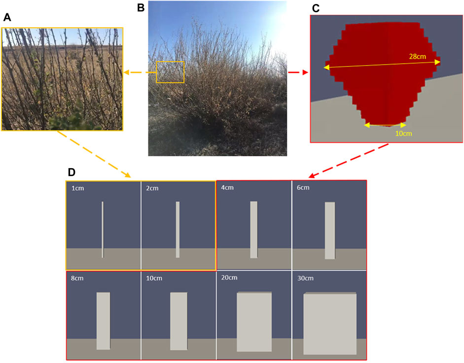
Figure 1. From field observations to numerical simulations: (A) branches of Caragana in the field, (B) actual morphology of Caragana korshinskii (Bashang Grassland, Hebei Province) in the field, (C) realistic numerical simulation model of Caragana, and (D) branch model (1 cm, 2 cm) and simplified model (4, 6, 8, 10, 20, and 30 cm) in numerical simulation.

Figure 2

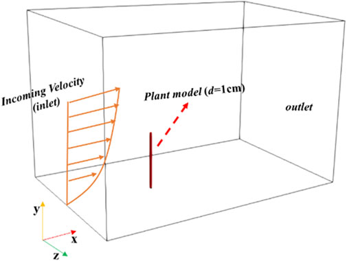
Figure 2. Computational domain of numerical simulation for the cuboid model with d = 1 cm.

The boundary conditions are set based on previous numerical simulations (Guo et al., 2021; Wu et al., 2022; Wu et al., 2023) and wind-tunnel tests (Wu et al., 2015) of windbreaks and are shown in Supplementary Table S1 in detail. This study was mainly concerned with the swinging of the model so as to observe and record the evident swinging of the model, and a high wind velocity of 20 m/s (at the height of 60 cm) was applied to the inlet boundary.

To analyze the accuracy of the simulation results of flexible plants, we simulated a rigid model for comparison. For the numerical simulation of the rigid model, we used the same geometric model, and only the RANS turbulence model was used. The other parameters are consistent with that of the flexible models, and the case of the rigid model is solved by the transient solver simpleFoam.

2.1.2 Governing equations for the turbulence flow

The RANS (Wilson, 1985) method was used to solve the problem of the turbulence simulation in our study. OpenFOAM provides many turbulence models for simulating the wind speed near the surface, which are also suitable for its extended version foam-extend.

The continuity and momentum equations of the RANS method are as follows (Bitog et al., 2009; Rosenfeld et al., 2010; Guo and Maghirang, 2012; Fang et al., 2018; Guo et al., 2021):

Continuity equation:

$\frac{\partial \overline{{\mathit{u}}_{\mathit{i}}}}{\partial x_i}=0.(1)$

Momentum equation:

$\frac{\partial \overline{{\mathit{u}}_{\mathit{i}}}}{\partial t}+\overline{{\mathit{u}}_{\mathit{j}}}\frac{\partial \overline{{\mathit{u}}_{\mathit{i}}}}{\partial x_j}=-\frac{1}{\rho }\frac{\partial \overline{p}}{\partial x_i}+\left(\mu +{\mu }_t\right)\frac{{\partial }^2\overline{{\mathit{u}}_{\mathit{i}}}}{\partial x_j^2},(2)$

where x_i represents Cartesian coordinates (i = 1, 2, three; x₁ = x, x₂ = y, x₃ = z), u_i represents the respective velocity components (i =1, 2, 3), t is the time, p is the pressure, ρ is the density, μ is the dynamic viscosity (1.79 × 10⁻⁵ m² .s⁻¹), and ${\mu }_t$ is the turbulent viscosity.

The simplest and most complete turbulence model of the double equations includes the standard k-ε, RNG k-ε, and reliable k-ε models. Based on previous research studies (Jones and Launder, 1972; Launder and Sharma, 1974), the standard k-ε model is widely used due to its robustness and reasonable accuracy for a wide range of flows. In particular, in the numerical simulation of wind and sand flows, it is relatively economic, accurate, and can effectively solve the problem of airflow field around the windbreaks (Milliez and Carissimo, 2007; Rosenfeld et al., 2010; Guo and Maghirang, 2012; Lima et al., 2017). Therefore, the standard k-ε model was used in our study. In the standard k-ε model, the wall function is used to simplify the wall treatment, which has a good convergence rate and relatively low memory demand. The model solves two variables, namely, turbulent kinetic energy k) and kinetic energy dissipation rate ε), and is calculated using Eqs 3, 4 (Santiago et al., 2007; Bourdin and Wilson, 2008; Fang et al., 2018):

$\frac{\partial }{\partial t}\left(\rho k\right)+\frac{\partial }{\partial x_i}\left(\rho k{\mathit{u}}_{\mathit{i}}\right)=\frac{\partial }{\partial x_j}\left[\left(\mu +\frac{{\mu }_t}{{\sigma }_k}\right)\frac{\partial k}{\partial x_j}\right]+G_k+G_b-\rho \epsilon -Y_M+S_k,(3)$

$\frac{\partial }{\partial t}\left(\rho \epsilon \right)+\frac{\partial }{\partial x_i}\left(\rho \epsilon {\mathit{u}}_{\mathit{i}}\right)=\frac{\partial }{\partial x_j}\left[\left(\mu +\frac{{\mu }_t}{{\sigma }_{\epsilon }}\right)\frac{\partial \epsilon }{\partial x_j}\right]+G_{1\epsilon }\frac{\epsilon }{k}\left(G_k+C_{3\epsilon }{G}_b\right)-C_{2\epsilon }\rho \frac{{\epsilon }^2}{k}+S_{\epsilon },(4)$

where $G_k$ represents the turbulent kinetic energy terms generated by the laminar velocity gradient; $G_b$ represents the turbulent kinetic energy terms from buoyancy; $Y_M$ is the dissipative term of the compressible fluid; $S_k$ and $S_{\epsilon }$ are user-defined source items; ${\sigma }_{\epsilon }$ and ${\sigma }_k$ are the numbers of turbulent Prandtl k and ε equations, respectively; the default initial value is constant, ${\sigma }_{\epsilon }$ = 1.0, ${\sigma }_k$ = 1.3; $C_{1\epsilon }$, $C_{2\epsilon }$, and $C_{3\epsilon }$ are constants; and $C_{1\epsilon }$ = 1.44, $C_{2\epsilon }$ = 1.92, and $C_{3\epsilon }$ = $C_{\mu }$ = 0.09.

The initial values of k and ε can be calculated from Eqs 5, 6 (Li et al., 2007):

$k^{*}=\frac{u^{*2}}{\sqrt{C_{\mu }}},(5)$

${\epsilon }^{*}=\frac{u^{*3}}{\kappa z},(6)$

where $C_{\mu }$ is a constant of 0.09, κ is a von Kaman constant, and the value is 0.4187.

2.1.3 Fluid–structure interaction

In the study of the fluid–structure interaction between airflow and flexible plants, the governing equation of the fluid follows the continuity and momentum conservation equations. The structural features of flexible plants can be described using a 3D geometry; hence, there is no need to add momentum source terms (Fang, 2019). In this study, flexible plants are considered adiabatic linear elastic solid materials. Under the action of wind, plants undergo significant deformation. According to the computational solid mechanics principle, the governing equations for a solid can be written as follows (Fang, 2019):

${\displaystyle \underset{{\mathrm{\Omega }}_0}{\int }}{\rho }_{s0}\frac{\partial {\mathit{u}}_{\mathit{s}}}{\partial t}d{\mathrm{\Omega }}_0={\displaystyle \underset{{\mathrm{\Gamma }}_0}{\int }}{n}_0\cdot \left(2{\mu }_s+\lambda \right)\nabla d_{s}d{\mathrm{\Gamma }}_0+{\displaystyle \underset{{\mathrm{\Gamma }}_0}{\int }}{n}_0\cdot qd{\mathrm{\Gamma }}_0+{\displaystyle \underset{{\mathrm{\Omega }}_0}{\int }}{\rho }_{s0}\frac{\partial {\mathit{f}}_{\mathit{b}}}{\partial t}d{\mathrm{\Omega }}_0,(7)$

where ${\rho }_{s0}$ represents the initial density of the solid, ${\mathit{u}}_{\mathit{s}}$ is the solid velocity vector, ${\mathrm{\Omega }}_0$ is the initial control body, ${\mathrm{\Gamma }}_0$ is the initial control surface, $n_0$ is the unit normal vector of the initial moment, $d_s$ is the solid displacement vector, ${\mathit{f}}_{\mathit{b}}$ is the volumetric force, and q is composed of non-linear and coupling terms, expressed as

$q={\mu }_s{\left(\nabla d_s\right)}^T+\lambda tr\left(\nabla d_s\right)I-\left({\mu }_s+\lambda \right)\nabla d_s+{\mu }_s\nabla d_s\cdot {\left(\nabla d_s\right)}^T+\frac{1}{2}\lambda \left(\nabla d_s:\nabla d_s\right)I+\left(S+\sigma \right),(8)$

where S represents the Piola–Kirchhoff second stress tensor, $\sigma$ is the Cauchy stress tensor, ${\mu }_s$ and λ represent the Lamé constants, and their relationship with the Young’s modulus (E) and Poisson’s ratio (${\nu }_s$), which characterize the plant flexibility, is as follows:

${\mu }_s=\frac{E}{2\left(1+{\nu }_s\right)},(9)$

$\lambda =\frac{{\nu }_s}{\left(1+{\nu }_s\right)\left(1-2{\nu }_s\right)}.(10)$

Based on the governing equations of the solid (Eq. 7) and fluid (Eqs 1, 2), we derived the fluid–solid coupling boundary condition at the boundary to make the physical quantities at the boundary reach equilibrium. On the fluid–solid boundary, the fluid flow velocity (${\mathit{u}}_{\mathit{f}}$) should be equal to the structural velocity (${\mathit{u}}_{\mathit{w}}$); the flow velocity (${\mathit{u}}_{\mathit{f}}$) of the fluid should be equal to the deformation rate $\left(\frac{\partial d_s}{\partial t}\right)$ of the structure, and the force (${\sigma }_s$) of the solid should be equal to the pressure and viscous force (${\tau }_f$) applied by the fluid to it. Therefore, the fluid–solid coupling equation at the boundary can be expressed as follows (Campbell and Paterson, 2011):

$\left\{\begin{array}{c}{\mathit{u}}_{\mathit{f}}={\mathit{u}}_{\mathit{w}}\\ {\mathit{u}}_{\mathit{w}}=\frac{\partial d_s}{\partial t}\\ {\mathit{\tau }}_{\mathit{f}}={\sigma }_s\end{array}\right..(11)$

This study uses a third-party tool FSI solver fsiFoam to solve the interaction between airflow and flexible plants in the OpenFOAM extended version Foam-extend environment. A finite volume method (FVM) is used to discretize the fluid equation. The PISO solver is used to solve the problem in our study. Its computational efficiency is relatively low, and it takes approximately 200 cores to calculate a case; thus, in total, it takes approximately 12,800 cores to calculate 64 cases in this study. A finite element method (FEM) is used to discretize the solid equation, and the Laplacian solver is used to solve it. The arbitrary Lagrangian Euler (ALE) method is used to solve the mesh movement at the interface. The information interaction between the fluid and solid at the interface is realized using the GGI interface. During the calculation, Co is kept at approximately 1.6, and the convergence standard of each physical quantity is ${10}^{-6}$.

2.2 Evaluation and analysis

The rationality of the numerical simulation was evaluated from qualitative and quantitative aspects. Qualitatively, we evaluated the rationality of the numerical simulation results of a single flexible plant model on the basis of the rigid model simulation results. The geometry and simulation parameters of the rigid model are completely consistent with those of the flexible model but are solved using the transient solver simpleFoam. Furthermore, it was qualitatively analyzed by the flow field structure and wind speed change in the downwind direction.

To directly compare the effect of flexible and rigid plants on the airflow field, the commonly used logarithmic wind velocity profile (Kaimal and Finnigan, 1994; Dong et al., 2007) was applied at the inlet boundary:

${\mathit{u}}_{\mathit{z}}=\frac{u_{*}}{\kappa }\bullet \mathit{ln}\left(\frac{z}{z_0}\right),(12)$

where $u_z$ denotes the incoming velocity for the height of z. $u_{*}$ denotes friction velocity (set as 0.4 m/s) (Bourdin and Wilson, 2008); $\kappa$ denotes the von Karman constant (set to 0.4), and $z_0$ denotes surface roughness (set as ${10}^{-4}\mathrm{m}$) (Fang et al., 2018).

To evaluate the flexibility changes, according to the definition of psammophytes provided by Qu et al. (2012), their branches have certain toughness and, therefore, swing and bend along the wind direction under the action of wind. Hence, the swing amplitude (β) is defined to evaluate the variation in the flexibility. β refers to the swing angle between the initial and swing positions when the maximum swing of the model occurs within 2 s (which is the simulation time of the cases in this study). The unit of β is°, and the specific measurement is shown in Figure 3.

Figure 3

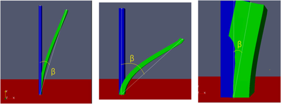
Figure 3. Specific measurement of the swing amplitude (β).

The reduction coefficient ${\text{Rc}}_{\left(x,z\right)}$ (Cornelis and Gabriels, 2005) is used to focus on the degree of wind speed reduction, and it is also a common way to evaluate the deceleration effect (Wu et al., 2015):

${\text{Rc}}_{\left(x,z\right)}=1-\frac{u_{x,z}}{u_{0\left(x,z\right)}},(13)$

where x is the horizontal distance from the model, z is the height, $u_{0\left(x,z\right)}$ is the time-averaged velocity when there is no plant shelter in the domain, and $u_{x,z}$ is the time-averaged velocity decreased by the plant and lower than $u_{0\left(x,z\right)}$. Generally, the deceleration effect increases as Rc_{(x, z)} increases.

3 Result

3.1 Comparison between flexible and rigid plants

We validated the rationality of the simulation method by comparing the similarities and differences in the airflow field between the flexible and rigid models. We take the simplified model (d = 4 cm) as an example. Figure 4 shows the airflow field around the two models. Figures 4A–D show the vertical airflow fields around the rigid and flexible models, respectively. Figure 4E,G and Figure 4F,H show the horizontal flow around the rigid and flexible models, respectively. The airflow fields around the rigid and flexible models before starting to swing are shown in Figure 4A,C and Figure 4E,G, respectively. At this time, the airflow fields around the two models are largely consistent. When the flexible model begins to swing under the action of the wind, the airflow field around it changes and the difference between the flexible and rigid models is noticeable. When the flexible model swings and reaches the maximum swing amplitude, the airflow fields around the rigid and flexible models are shown in Figure 4B,D and Figure 4F,H, respectively. At this time, the airflow field around the two models has been fully developed in the simulation domain. The airflow fields around the two models are similar: different colors represent different airflow zones (Plate, 1971; Judd et al., 1996; Guo et al., 2021) of the airflow field (Figure 4). However, compared with the rigid model (Figures 4A,C,E,G), the size of the different airflow zones in the leeward side of the flexible model changes to a certain extent (Figure 4B,D,F,H). The variation in each zone of the airflow field is closely related to the swing of the model. The airflow field at the horizontal plane (Figures 4G,H) shows that the maximum near-surface wind velocity around the flexible model is lower than that of the rigid model (the maximum wind velocity around the rigid model is 10.92 m/s in Figure 4G and 10.89 m/s around the flexible model in Figure 4H), i.e., Supplementary Figure S3 (Supplementary Material) shows the difference in ${\text{Rc}}_{\left(x,z\right)}$ near the ground between the rigid and flexible models in the downwind direction. It can be seen that the deceleration effect in the downwind direction of the flexible model is superior to that of the rigid model. The flexibility is more effective than rigidity for plants in terms of velocity reduction. Therefore, based on a qualitative analysis, the airflow field around the flexible model is found to be reasonable, and it also proves the correctness of our simulation method.

Figure 4

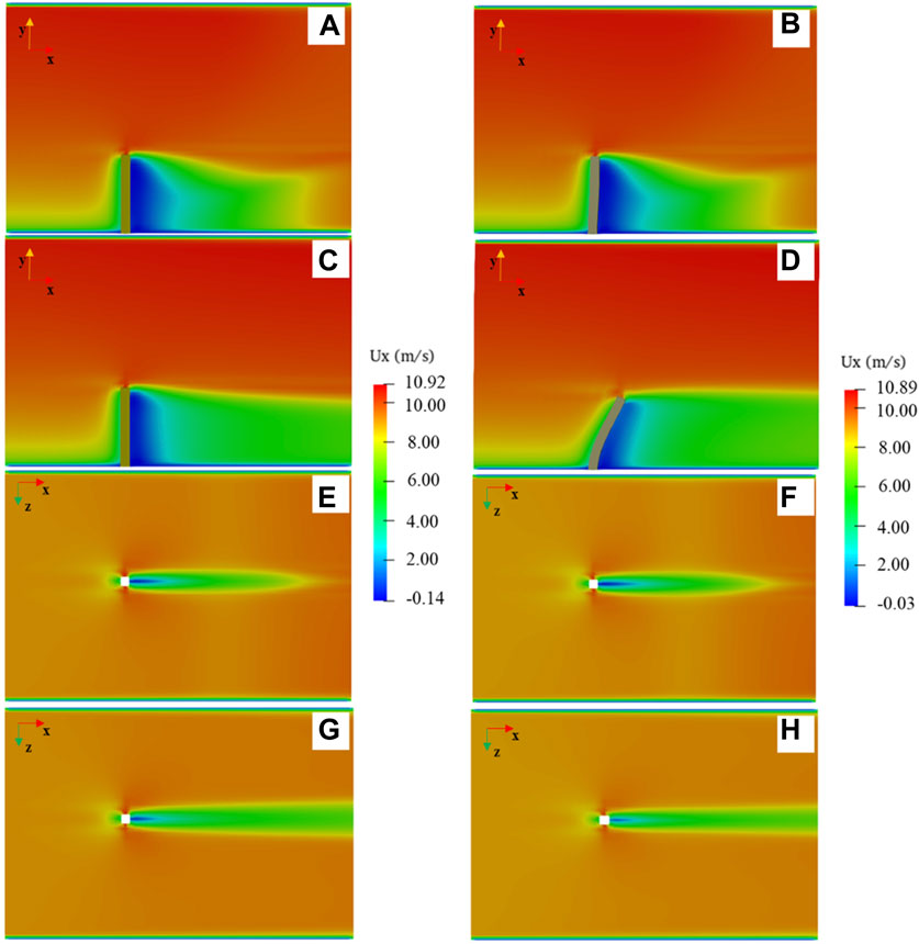
Figure 4. Velocity components in the x direction around the plant: (A–D) at the vertical plane z = 0, where (A) the airflow field around the rigid model at the initial position, (B) airflow field around the flexible model at the initial position, (C) airflow field around the rigid model when the flexible model reaches the maximum swing position, (D) airflow field around the flexible model at the maximum swing position, (E–H) at the horizontal plane y = 0.5 h, where (E) airflow field of the rigid model at the initial position, (F) airflow field around the flexible model at the initial position, (G) airflow field of the rigid model when the flexible model reaches the maximum swing position, and (H) airflow field around the flexible model at the maximum swing position.

3.2 Swing amplitude of flexible models with different diameters

3.2.1 Branch models (d = 1, 2 cm)

According to Zuo et al. (2015), there is a negative correlation between the Young’s modulus and the branch diameter. In our study, the Young’s modulus of the branches with a diameter of 1 cm ranges from 3 × 10⁷ to 1 × 10⁸ N .m⁻². Thus, for a uniform final swing amplitude interval, each interval of 1 × 10⁷ N .m⁻² is simulated. Similarly, the Young’s modulus of the branch model with a diameter of 2 cm is set ranging from 3 × 10⁶ to 1 × 10⁷ N .m⁻², with the same interval, with each interval being 1 × 10⁶ N .m⁻², and eight cases are simulated in total. Finally, for a wind velocity of 20 m/s, the Young’s modulus values of the two models and the corresponding swing amplitude measured are listed in Table 1.

Table 1

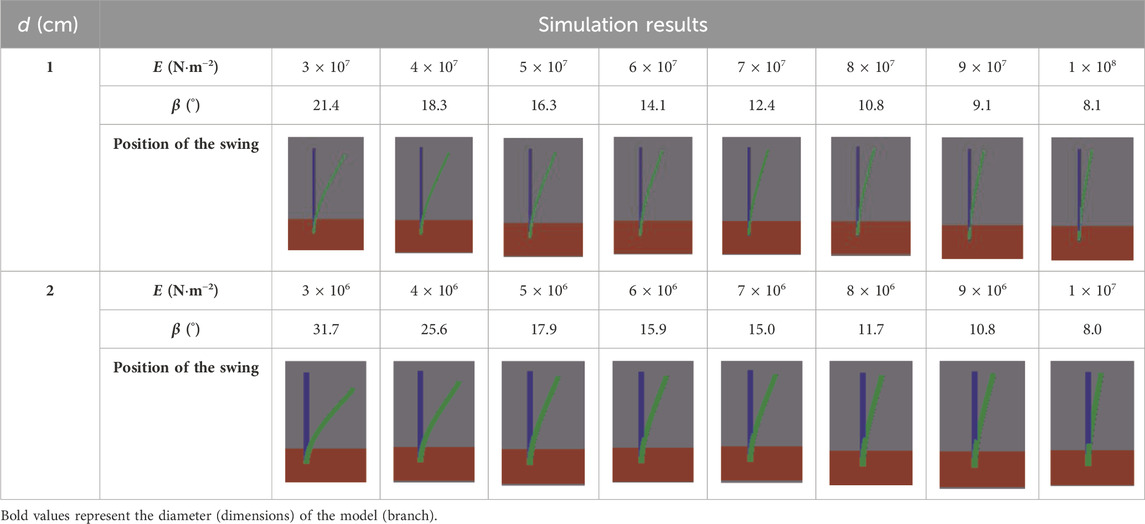
Table 1. Comparison between the maximum swing position of the branch models and their initial position under an incoming wind velocity of 20 m/s (blue, initial position; green, maximum swing position).

According to Table 1, the Young’s modulus of the branch model with a diameter of 1 cm decreases by 13.3° from 3 × 10⁷ to 1 × 10⁸ N .m⁻², and the gap of β is 3.1°–1° per interval of 1 × 10⁷ N .m⁻²; the Young’s modulus of the branch model with a diameter of 2 cm changes from 3 × 10⁶ to 1 × 10⁷ N .m⁻², and the swing amplitude of the Young’s modulus varies by 7.7°–0.9° per interval of 1 × 10⁶ N .m⁻². The results illustrate that for the plant branches, with the increase in the Young’s modulus, the swing amplitude decreases, that is, the flexibility of the branches decreases. Therefore, the branches of flexible psammophytes will swing under the action of the wind. When β reaches 10.8°, the Young’s modulus of the 1 cm-diameter branch model is 8 × 10⁷ N .m⁻², whereas that of the 2 cm-diameter branch model is 9 × 10⁶ N .m⁻². This illustrates that the Young’s modulus of the larger model is lower than that of the smaller model when the swing amplitude is similar. When the two models reach similar swing amplitudes of 8.1° and 8°, respectively, the Young’s modulus is quite different. The Young’s modulus of the branch model with a diameter of 1 cm is 1 × 10⁸ N .m⁻² and that of the branch model with a diameter of 2 cm is 1 × 10⁷ N .m⁻². This implies a quantitative relationship between the Young’s modulus and the diameter of the branch model. To explore this relationship, we conducted more sets of numerical simulations, as reported in the following.

3.2.2 Simplified models (d = 4, 6, 8, 10, 20, and 30 cm)

Based on the simulation of the two branch models, we found that to achieve an approximate swing amplitude, the Young’s modulus required for a larger-diameter branch model is slightly lower than that required for a branch model with a smaller diameter. Therefore, to establish the relationship of the Young’s modulus between the branch model and the simplified model with a large diameter, we set up six simplified models (d = 4, 6, 8, 10, 20, and 30 cm, respectively). Based on the abovementioned qualitative relationship between the Young’s modulus and the swing amplitude of the branch model, the Young’s modulus is reduced appropriately, and a series of numerical simulations are conducted on each set of simplified models. We record each Young’s modulus corresponding to the swing amplitude of the simplified models. Finally, we chose the groups (1–8) of the simplified models, which are close to the branch model, for the analysis to obtain the appropriate value of the Young’s modulus. We selected the swing amplitude close to the branch model in each group and the corresponding Young’s modulus. Table 2 lists the analysis results of the simplified models.

Table 2

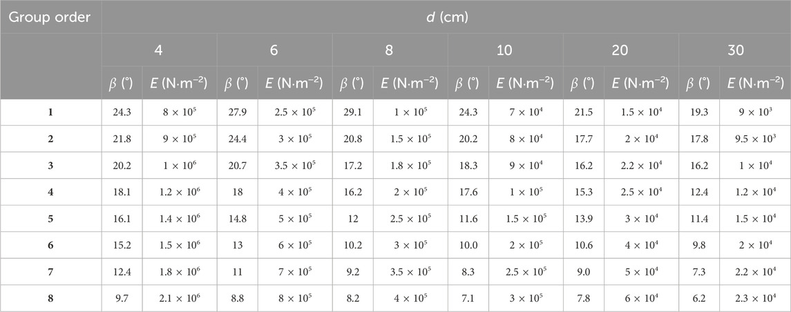
Table 2. Swing amplitude (β) and Young’s modulus (E) of the simplified models.

Table 2 lists the specific swing amplitude and the corresponding Young’s modulus. The swing amplitude of the simplified model is between 29.1° and 6.2° (Table 2), whereas the swing amplitude of the branch model is between 31.7° and 8.0° (Table 1). The maximum gap between them is only 2.6°. Therefore, the range of the swing amplitude between the two types of models is similar. From Table 2, we find that the swing amplitude increases with the decrease in the Young’s modulus at each diameter level, which is consistent with the numerical simulation results of the branch model (Table 1). Moreover, with the increase in the diameter, the Young’s modulus decreases evidently when the approximate swing amplitude is reached. When β is 18.3°, the Young’s modulus of the branch model with a diameter of 1 cm is 4 × 10⁷ N .m⁻². When β is close to 18.3° (Table 1), for the simplified model with d = 4 cm (Table 2), the Young’s modulus is 1.2 × 10⁶ N .m⁻² (β = 18.1°); for the model with d = 6 cm (Table 2), the Young’s modulus is 4 × 10⁵ N .m⁻² (β = 18°); for the model with d = 10 cm (Table 2), the Young’s modulus is 9 × 10⁴ N .m⁻² (β = 18.3°). When the swing amplitude of the simplified models is close to that of the branch models, the Young’s modulus of the simplified models is much lower than that of the branch model, given the larger diameter.

Based on the above analysis, for both the branch and simplified models, the swing amplitude decreases with the increase in the Young’s modulus under the same diameter; and the Young’s modulus decreases as the diameter increases when the same swing amplitude is obtained. Furthermore, there exists a negative relationship among swing amplitude, model diameter, and Young’s modulus. Therefore, we further investigated this relationship based on the results listed in Table 1 and Table 2.

3.3 Establishment of Young’s modulus

At a wind velocity of 20 m/s, for the branch model with a diameter of 1 cm, the Young’s modulus is between 3 × 10⁷ N .m⁻² and 1 × 10⁸ N .m⁻², and the corresponding swing amplitude range is 21.4°–8.1°; for the branch model with a diameter of 2 cm, the Young’s modulus range is 3 × 10⁶–1 × 10⁷ N .m⁻², and the corresponding swing amplitude range is 31.7°–8°. At the same wind velocity, the swing amplitude and corresponding Young’s modulus for the simplified models are also listed in Table 2. For example, the swing amplitude of the model (d = 4 cm) is between 24.3° and 9.7°, and the corresponding Young’s modulus is between 8 × 10⁵ N .m⁻² and 2.1 × 10⁶ N .m⁻². From the simulation results of the branch and simplified models, the maximum swing amplitude of 31.7° is observed for the branch model (d = 2 cm) (Table 2), whereas the minimum swing amplitude of 6.2° is observed for the simplified model with a diameter of 30 cm (Table 2). When the swing amplitude is 1° at each interval, the Young’s modulus intervals of the model (d = 1, 2, 4, 6, 8, 10, 20, and 30 cm) are approximately 5.3 × 10⁶, 3.0 × 10⁵, 1.1 × 10⁵, 2.9 × 10⁴, 1.4 × 10⁴, 1.3 × 10⁴, 3.3 × 10³, and 1 × 10³ N .m⁻², respectively. Therefore, when the models with different diameter levels swing in the numerical simulation, the required Young’s modulus is different. We draw the scatter plot between the Young’s modulus and the swing amplitude at different diameter levels (Figure 5). Evidently, as the Young’s modulus increases, the corresponding swing amplitude decreases. The corresponding Young’s modulus decreases as the model diameter increases if the same swing amplitude is obtained. This indicates that the Young’s modulus increases and that the deformation degree of the model decreases, which is in accordance with the definition of the Young’s modulus.

Figure 5

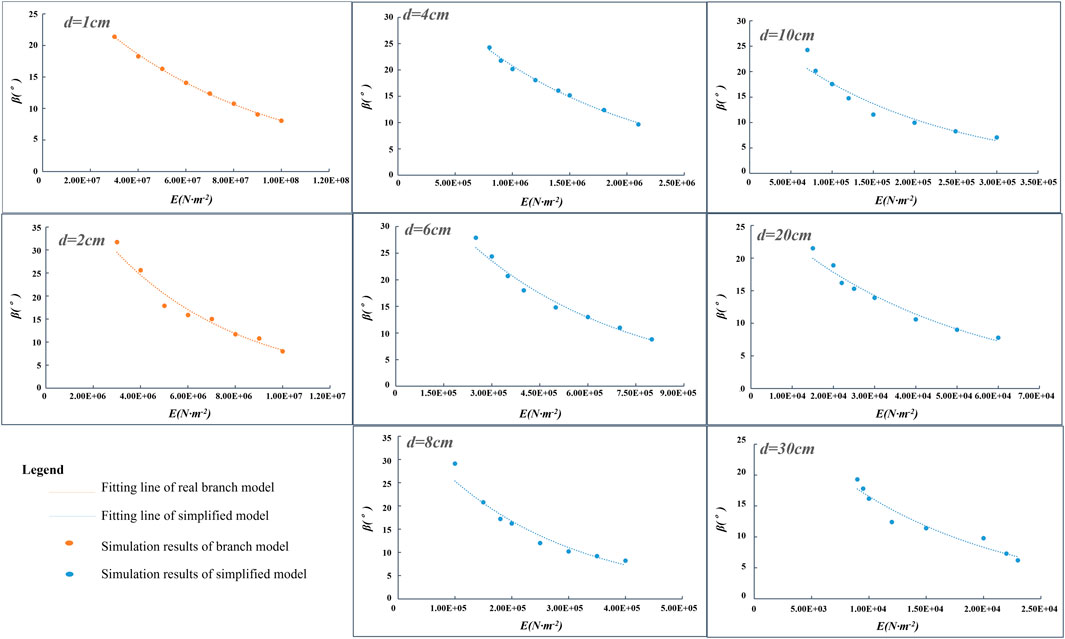
Figure 5. Relationship between the swing amplitude and Young’s modulus of flexible models with different diameters under a wind velocity of 20 m/s.

Figure 5 shows that there is an evident exponential function relationship between the swing amplitude and the Young’s modulus. The fitting degree of the regression equation is high, and all the values of R² are above 0.94; particularly when d = 1 cm, R² reaches 0.99. The specific fitting equation and the values of R² for all the models are shown in Supplementary Table S2 (Supplementary Material). The fitting equation of the curve in Figure 5 can be used to speculate the relationship between the swing amplitude and the Young’s modulus of the models with different diameters. Because all the dependent variables in the regression equation are swing amplitudes, the relationship between the branch model with d = 1 cm and the simplified model at different diameter levels can also be established when the swing amplitude is equal. Taking the simplified model with d = 8 cm as an example, by combining the fitting equation for d = 1 cm with the fitting equation for d = 8 cm, the relationship between the Young’s modulus of the simplified model and that of the branch model (d = 1 cm) can be obtained as follows:

$E_8=42604+0.0025*E_1,(14)$

where E₈ is the Young’s modulus of the simplified model (d = 8 cm) and E₁ is the Young’s modulus of the branch model (d = 1 cm).

Similar to the simplified model (d = 8 cm), the relationship between the Young’s modulus of the branch model and the Young’s modulus of the other simplified models (the specific functional relationship is also shown in Supplementary Table S2 of Supplementary Material) can also be obtained by fitting equations. In other words, when a plant is simulated as a complete geometric model, the Young’s modulus of the model can be calculated on the basis of the plant diameter and Eq. 14.

Therefore, when the Young’s modulus of the flexible plant model is considered in the numerical simulation, the above relationship can be referred on the basis of the different methods of model construction. This also provides a preliminary reference for the selection of the Young’s modulus.

3.4 Validation and application

An appropriate inlet boundary condition ensures the reliability of the numerical simulation. In our simulations, a logarithmic wind velocity profile was imposed as the incoming velocity to represent realistic field conditions, which makes it necessary to verify the rationality of the wind velocity profile. We compared simulated wind velocities at the inlet boundary with those measured in the wind tunnel (Wu et al., 2015). As shown in Supplementary Figure S1 (Supplementary Material), it proved that the initial conditions at the inlet boundary were quite reliable.

In the field, the wind speed of 10 m/s is more common than 20 m/s, and branches with a diameter of 1 cm are typically observed in real shrubs (Figure 1B). Therefore, for the branch model (d = 1 cm), we carry out a numerical simulation under a wind speed of 10 m/s to verify the correctness of the Young’s modulus used. Figure 6 shows the corresponding swing amplitude at 10 m/s with the same Young’s modulus under 20 m/s. When the Young’s modulus values are 3 × 10⁷, 4 × 10⁷, 5 × 10⁷, 6 × 10⁷, 7 × 10⁷, 8 × 10⁷, 9 × 10⁷, and 1 × 10⁸ N .m⁻², the swing amplitudes of the branch model (d = 1 cm) at 10 m/s are 6.7°, 5.3°, 4.5° 3.9°, 3.3°, 2.4°, 2.0°, and 1.7°, respectively. Compared with the swing amplitude at 20 m/s (Table 1), the swing amplitude at 10 m/s is evidently reduced. The range of the swing amplitude is reduced from 21.4°–8.1° to 6.7°–1.7°. At 10 m/s, the branches swing a certain degree in the field, and for the branch model (d = 1 cm), the swing amplitude is not high. Therefore, the simulation results are consistent with the actual situation. This indicates that the range of our Young’s modulus is logical.

Figure 6

Figure 6. Comparison of the maximum swing position of the branch model (d = 1 cm) under different wind velocities (blue, model initial position; green , maximum swing positions of the model under wind velocities of 10 m/s and 20 m/s, respectively).

We further verify the relationship derived above. First, the Young’s modulus of the branch model with a diameter of 1 cm is set to 5.9 × 10⁷ N .m⁻². On the basis of Eq. 14, it can be calculated that when the same swing amplitude is reached, the Young’s modulus of the simplified model with a diameter of 8 cm is approximately 1.90 × 10⁵ N .m⁻². Moreover, when the Young’s modulus values are 5.9 × 10⁷ N .m⁻² (d = 1 cm) and 1.90 × 10⁵ N .m⁻² (d = 8 cm), respectively, the swing amplitude of the model (d = 1 cm and d = 8 cm) should be approximately 15.0°. For the calculated values, we verified the accuracy by numerical simulation and observed the simulation results to check whether the model destabilizes and whether the corresponding swing amplitude is reached. Next, we set the Young’s modulus of the branch model with a diameter of 1 cm to be 5.9 × 10⁷ N .m⁻² and the Young’s modulus of the simplified model with a diameter of 8 cm to be 1.90 × 10⁵ N .m⁻². Two sets of numerical simulations were conducted, and results were obtained (Figure 7).

Figure 7

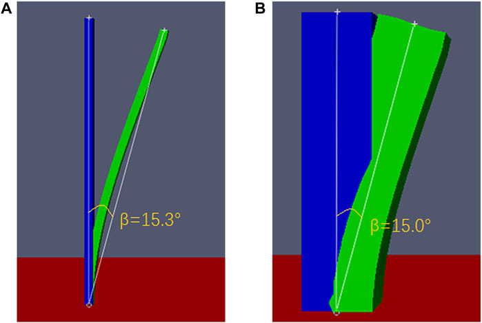
Figure 7. Swing amplitude of the models under a wind velocity of 20 m/s: (A) branch model (d = 1 cm), with a Young’s modulus of 5.9 × 10⁷ N .m⁻², and (B) simplified model (d = 8 cm), with a Young’s modulus of 1.90 × 10⁵ N .m⁻².

Figure 7 shows that when the Young’s modulus of the branch model with d = 1 cm is 5.9 × 10⁷ N .m⁻² and that of the simplified model with d = 8 cm is approximately 1.90 × 10⁵ N .m⁻², the corresponding swing amplitudes are 15.3° (Figure 7A) and 15.0° (Figure 7B), respectively. These values are close/equal to 15.0°. By comparing the simulation results of the models with d = 1 cm and 8 cm in Tables 1,2, we find that the results obtained conform to the logical relationship of the data in Supplementary Table S3. Therefore, it is proven that the relationship derived above is correct. Next, we apply this relationship to the realistic model of Caragana mentioned above (Figure 1C). Based on the above, since the minimum width at the bottom of the simplified model is 10 cm, it is reasonable to speculate that if the realistic model should exhibit a swing amplitude similar to that of branches at a wind speed of 20 m/s, its Young’s modulus should be equal to that between the 10-cm and 30-cm-diameter simplified models. Since the bottom of the model is 10 cm, i.e., the width of the plant root is 10 cm, the Young’s modulus value should be closer to that of the simplified model with a diameter of 10 cm. According to Table 2 and Eq. 13, we select the Young’s modulus of the realistic model as 8 × 10⁴ N .m⁻² for the numerical simulation. The other conditions are consistent with the previous numerical simulations, and the case is simulated under the same computational domain, as shown in Figure 4. At a wind speed of 20 m/s, the realistic model destabilizes; Figure 8 shows the magnitude of the swing amplitude.

Figure 8

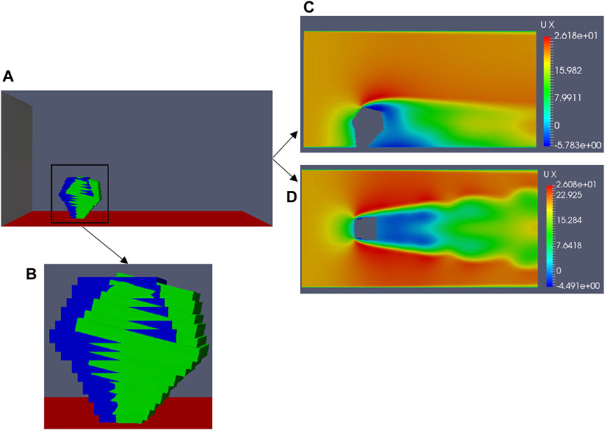
Figure 8. Under a wind velocity of 20 m/s, the realistic model reaches the maximum swing: (A) simulation domain, (B) maximum swing of the model compared with the initial position (blue, initial position; green, maximum swing position), (C) airflow field around the model at the vertical plane z = 0, and (D) airflow field around the model at the horizontal plane y = 0.1 h.

Figure 8A shows that when the Young’s modulus is 8 × 10⁴ N .m⁻², the maximum swing amplitude of the realistic model is 15.9° at a wind speed of 20 m/s (Figure 8B). Figures 8C, D show the airflow field surrounding the model. The airflow field around the realistic model is consistent with the airflow field around the branch model (d = 1 cm) (Figure 4), hence further proving the accuracy of the derived relationship.

4 Discussion

Although previous studies have defined flexible psammophytes (Tang et al., 2011; Qu et al., 2012), only few have reported methods to determine their flexibility. The Young’s modulus is an important index to evaluate flexibility. The values of Young’s modulus of the branches of some psammophytes species are given based on measurement experiments involving material mechanics (Zuo et al., 2015); the effect of plant geometry on the flexibility is not considered; furthermore, the Young’s modulus of the plant branches obtained based on the material mechanics was directly applied to the geometric model of the numerical simulation (Fang, 2019). Thus, this study uses the computational fluid dynamics (CFD) method and FSI model to clarify the relationship between the Young’s modulus values and the swing amplitude at different diameter levels based on the branch models (d = 1, 2 cm) and simplified models (d = 4, 6, 8, 10, 20, and 30 cm). Compared with previous studies, we made improvements in the following aspects. First, we measured the flexibility of the plant branches by focusing on the numerical changes in the Young’s modulus. Second, we simulated and analyzed the relationship between the swing amplitude and the Young’s modulus when the model swings at different diameter levels. We found that with the decrease in the Young’s modulus, i.e., an increase in the plant flexibility, the degree of bending and swinging of the plants increases. This not only accords with the definition of flexible psammophytes (Qu et al., 2012) but also advances our understanding of flexible psammophytes. Third, we not only paid attention to the Young’s modulus of the plant branches but also established the relationship between the Young’s modulus of the real branches and the simplified geometric model, on the basis of the relationship between the swing amplitude and the Young’s modulus. Fourth, by comparing with the simulation results of rigid plants, the rationality of our numerical simulation methods is proven. Moreover, based on the verification of the established relationship, we directly applied the results to the realistic model. This can provide a reference for determining the flexibility of other psammophytes.

It is known that plant coverage, shape, canopy morphology, leaf area, and flexibility are the key factors of psammophytes in controlling soil wind erosion and desertification (Zhang et al., 2008; Liu et al., 2018; Liu et al., 2021). Quantifying these factors can effectively reflect the protective ability of plants; however, flexibility is the most difficult factor to quantify. Tang et al. (2011) found that when airflow passes through rigid plants, plant branches swing less with airflow, the amount of the wind–sand flow settlement and accumulation is large, and the plants have a high capacity for sand interception. Flexible plants tend to deform and bend with a significant swing amplitude as airflow passes through them, but only a small wind–sand flow is intercepted. Thus, flexible plants’ capacity to intercept blowing sand is not very strong. This was also supported by Abulaiti et al. (2016), who suggested that rigid rough elements retained more sand particles than flexible plants. However, the swing of flexible plants also disturbs the airflow, weakens the wind speed, and renders the sand settle (Qu et al., 2012). Therefore, it is noteworthy that the selection of psammophytes with appropriate flexibility is important in the practical wind erosion and sand interception control. Tang et al. (2011) only qualitatively classified psammophytes into rigid and flexible plants, and they believed that a method to scientifically determine the flexibility of plant stems and branches and quantitatively grade the flexibility is a focus for future research. Kang et al. (2019) conducted a wind-tunnel test on flexible plants using the artificial plastic flexible plant and rigid plants with cube and cylinder blocks. They found that normalized aerodynamic roughness (ratio of aerodynamic roughness to plant height) of the flexible plant is significantly lower than that of rigid plants. Based on the field observation, Zhang et al. (2022) found that when wind speed increases, flexible roughness elements’ ability becomes stronger in reducing soil wind erosion. This was related to the porosity and height of flexible plants but did not elaborate on the impact of flexibility. Liu et al. (2021) replaced flexible plants with regular rough elements with the same shape in a wind-tunnel test and only studied the shape effects of plants. They also suggested that it was necessary to study the influence of flexibility on plant sand resistance. To represent the effect of flexible vegetative windbreak on airflow, Liu et al. (2021) proposed a correction factor in the source terms of the momentum and turbulence transport equations. Although previous studies have qualitatively pointed out the importance of flexibility or parameterized the effect of the plant flexibility, there are rare quantitative studies directly specifying the flexibility of psammophytes.

Thus, based on the numerical simulation in this study, by establishing the functional relationship between Young’s modulus and swing amplitude, and the Young’s modulus relationship between real branches and plant models, we provide different flexibilities to plant models in numerical simulation, which provides a new reference for the quantitative study of psammophyte flexibility, and the flexibility can be expressed by the change of swing amplitude so as to realize the graded evaluation of flexibility. Based on the Young’s modulus relationship between branches with different diameters and the numerical simulation models, different flexibilities can be provided to different plant models. The effect of flexibility on wind prevention of psammophytes can be quantitatively evaluated by calculating the shelter distance, the minimum wind speed, and the turbulence intensity in the downwind, and that on sand interception can also be quantitatively evaluated by calculating the shear force and the sediment transport rate under different flexibility. Therefore, we can evaluate the ability of wind erosion and sand resistance of psammophytes in different real-world situations (such as different prevailing wind velocities and different underlying surfaces) and can also explain the difference of wind erosion reduction between rigid and flexible plants by comparing other components of velocity field, turbulence characteristics, and the pressure field of rigid and flexible plant stems and branches, which are exactly the research work we will carry out in the future. Therefore, this study has practical significance in the control of wind erosion and sand deposition.

Our study has some limitations. First, in practice, the shape of the plant branches is more cylindrical and comprises two parts, namely, a branch and canopy; however, to ensure the strict fit and interaction of the branches at the airflow interface during the fluid–structure interaction, we can only use regular structured meshes to simulate them as a complete geometry with small cuboid. Second, this study is a preliminary exploratory study on the flexibility of psammophytes. Only using Young’s modulus as the evaluation index of the flexibility of one shrub, we mainly evaluate the swing amplitude and did not consider the other factors, such as the wind speed change in the downwind direction or the surface shear force. Third, due to the complexity of the fluid–structure interaction and the inability to build a real plant canopy model, the difference between erect and sloping branches could not be compared. Finally, there is a lack of validation that matches the swing amplitude of flexible plants with wind-tunnel experimental data as it is difficult to obtain the instantaneous swing characteristics of plants in both field observations and wind-tunnel experiments. Therefore, in the future, we will further our study from these aspects and more thoroughly study the flexibility range of various psammophytes and the interaction between a single flexible plant and the surrounding airflow field, thus providing a clearer reference for the application of flexible psammophytes in sand control engineering.

5 Conclusion

In this study, based on a 3D computational fluid dynamics (CFD) simulation, we used the standard k-ε turbulence model and FSI model to simulate the airflow around a series of psammophyte branch models and simplified models. By simulating the swing of real branches with different Young’s modulus, in the airflow field, and taking the swing amplitude as the evaluation index, we intuitively established the relationship between the Young’s modulus of the real branches and that of the simplified plant model in the numerical simulation. After analyzing and comparing the simulation results of the rigid model and the flexible models under different wind speeds, we found, under the same wind speed, the swing amplitude of the model decreases with an increase in the Young’s modulus. Furthermore, a negative exponential function relationship is developed between these two parameters. Similarly, at the same wind speed, when reaching the same swing amplitude as the real branch, the larger the model size, the lower the Young’s modulus. This study represents a first step toward the qualitative investigation of plant flexibility. If the relationship between real psammophytes and the Young’s modulus of the corresponding models is considered in the numerical simulation, future researchers can refer to the relationship derived in this study.

Data availability statement

The original contributions presented in the study are included in the article/Supplementary Material; further inquiries can be directed to the corresponding author.

Author contributions

HX: formal analysis, methodology, project administration, visualization, writing–original draft, and writing–review and editing. XW: funding acquisition, resources, supervision, writing–review and editing, conceptualization, and writing–original draft. RW: funding acquisition, investigation, resources, supervision, and writing–review and editing. CS: supervision and writing–review and editing. HF: methodology, software, and writing–review and editing. XZ: supervision and writing–review and editing. ZG: investigation, methodology, and writing–review and editing. JY: investigation and writing–review and editing. XL: supervision and writing–review and editing. XY: supervision and writing–review and editing.

Funding

The author(s) declare that financial support was received for the research, authorship, and/or publication of this article. This work was financially supported by the National Natural Science Foundation of China (grant nos 41871004 and 42077069).

Conflict of interest

The authors declare that the research was conducted in the absence of any commercial or financial relationships that could be construed as a potential conflict of interest.

Publisher’s note

All claims expressed in this article are solely those of the authors and do not necessarily represent those of their affiliated organizations, or those of the publisher, the editors, and the reviewers. Any product that may be evaluated in this article, or claim that may be made by its manufacturer, is not guaranteed or endorsed by the publisher.

Supplementary material

The Supplementary Material for this article can be found online at: https://www.frontiersin.org/articles/10.3389/fenvs.2024.1380498/full#supplementary-material

References

Abulaiti, A., Kimura, R., and Kodama, Y. (2016). Effect of flexible and rigid roughness elements on aeolian sand transport. Arid Land Res. Manag. 31, 111–124. doi:10.1080/15324982.2016.1260665

CrossRef Full Text | Google Scholar

Bitog, J. P., Lee, I. B., Shin, M. H., Hong, S. W., Hwang, H. S., Seo, I. H., et al. (2009). Numerical simulation of an array of fences in Saemangeum reclaimed land. Atmos. Environ. 43, 4612–4621. doi:10.1016/j.atmosenv.2009.05.050

CrossRef Full Text | Google Scholar

Bourdin, P., and Wilson, J. D. (2008). Windbreak aerodynamics: is computational fluid dynamics reliable? Boundary-Layer Meteorol. 126, 181–208. doi:10.1007/s10546-007-9229-y

CrossRef Full Text | Google Scholar

Campbell, R. L., and Paterson, E. G. (2011). Fluid-structure interaction analysis of flexible turbomachinery. J. Fluids Struct. 27 (8), 1376–1391. doi:10.1016/j.jfluidstructs.2011.08.010

CrossRef Full Text | Google Scholar

Chen, S., and Gu, X. (2017). Heart stent, origami art and metamaterial design. Sci. Technol. Guide 35, 105. (in Chinese).

Google Scholar

Cornelis, W. M., and Gabriels, D. (2005). Optimal windbreak design for wind-erosion control. J. Arid Environ. 61 (2), 315–332. doi:10.1016/j.jaridenv.2004.10.005

CrossRef Full Text | Google Scholar

Dong, Z., Mu, Q., and Wang, H. (2007). Wind velocity profiles with a blowing sand boundary layer: theoretical simulation and experimental validation. J. Geophys Res. Atmos. 112. doi:10.1029/2006JD007447

CrossRef Full Text | Google Scholar

Fang, H. (2019) Numerical simulation of airflow around wind barriers and flexible vegetation, (Master’s thesis). Beijing: Beijing Normal University. (in Chinese).

Google Scholar

Fang, H., Wu, X., Zou, X., and Yang, X. (2018). An integrated simulation-assessment study for optimizing wind barrier design. Agric. For. Meteorology 263, 198–206. doi:10.1016/j.agrformet.2018.08.018

CrossRef Full Text | Google Scholar

Gan, C. J., and Salim, S. M. (2014). “Numerical analysis of fluid-structure interaction between wind Flow and Trees,” in Proceedings of the world congress on engineering (London, U.K: IEEE).

Google Scholar

Gerile, H., Si, Q., and Liu, J. (2013). Branches tensile mechanical characteristics and the influencing factors of six plant species in Inner Mongolia. J. Desert Res. 33 (5), 1333–1339. (in Chinese).

Google Scholar

Grant, P. F., and Nickling, W. G. (1998). Direct field measurement of wind drag on vegetation for application to windbreak design and modelling. Land Degrad. Dev. 9, 57–66. doi:10.1002/(sici)1099-145x(199801/02)9:1<57::aid-ldr288>3.0.co;2-7

CrossRef Full Text | Google Scholar

Guan, D., Zhang, Y., and Zhu, T. (2003). A wind-tunnel study of windbreak drag. Agric. For. Meteorology 118, 75–84. doi:10.1016/S0168-1923(03)00069-8

CrossRef Full Text | Google Scholar

Guo, L., and Maghirang, R. G. (2012). Numerical simulation of airflow and particle collection by vegetative barriers. Eng. Appl. Comput. Fluid Mech. 6, 110–122. doi:10.1080/19942060.2012.11015407

CrossRef Full Text | Google Scholar

Guo, Z., Yang, X., Wu, X., Zou, X., Zhang, C., Fang, H., et al. (2021). Optimal design for vegetative windbreaks using 3D numerical simulations. Agric. For. Meteorology 108290, 108290–108299. doi:10.1016/j.agrformet.2020.108290

CrossRef Full Text | Google Scholar

Järvelä, J. (2002). Flow resistance of flexible and stiff vegetation: a flume study with natural plants. J. Hydrology 269 (1-2), 44–54. doi:10.1016/S0022-1694(02)00193-2

CrossRef Full Text | Google Scholar

Jones, W. P., and Launder, B. E. (1972). The prediction of laminarization with a two-equation model of turbulence. Int. J. Heat Mass Transf. 15 (2), 301–314. doi:10.1016/0017-9310(72)90076-2

CrossRef Full Text | Google Scholar

Judd, M. J., Raupach, M. R., and Finnigan, J. J. (1996). A wind tunnel study of turbulent flow around single and multiple windbreaks, part I: velocity fields. Boundary-Layer Meteorol. 80, 127–165. doi:10.1007/BF00119015

CrossRef Full Text | Google Scholar

Kaimal, J., and Finnigan, J. (1994) Atmospheric boundary layer flows. New York: Oxford University Press, 299–300.

Google Scholar

Kang, L., Yang, Z., Zhang, J., Zou, X., and Zhang, W. (2020). Wind tunnel simulation for comparison of wind velocity profile characteristics at two flexible plant surfaces. J. Desert Res. 40 (02), 43–49. (in Chinese).

Google Scholar

Kang, L., Zhang, J., Zou, X., Cheng, H., Zhang, C., and Yang, Z. (2019). Experimental investigation of the aerodynamic roughness length for flexible plants. Boundary-Layer Meteorol. 172 (3), 397–416. doi:10.1007/s10546-019-00449-0

CrossRef Full Text | Google Scholar

Kim, R. W., Lee, I. B., Kwon, K. S., Yeo, U. H., Lee, S. Y., and Lee, M. H. (2018). Design of a windbreak fence to reduce fugitive dust in open areas. Comput. Electron. Agric. 149, 150–165. doi:10.1016/j.compag.2017.08.014

CrossRef Full Text | Google Scholar

Kouwen, N., Unny, T. E., and Hill, H. M. (1969). Flow retardance in vegetated channels. J. Irrigation Drainage Div. 95 (02), 329–342. doi:10.1061/jrcea4.0000652

CrossRef Full Text | Google Scholar

Launder, B. E., and Sharma, B. I. (1974). Application of the energy-dissipation model of turbulence to the calculation of flow near a spinning disc. Lett. Heat Mass Transf. 1 (2), 131–137. doi:10.1016/0735-1933(74)90024-4

CrossRef Full Text | Google Scholar

Leenders, J. K., Boxel, J. H. V., and Sterk, G. (2007). The effect of single vegetation elements on wind speed and sediment transport in the Sahelian zone of Burkina Faso. Earth Surf. Process. Landforms 32, 1454–1474. doi:10.1002/esp.1452

CrossRef Full Text | Google Scholar

Li, W., Wang, F., and Bell, S. (2007). Simulating the sheltering effects of windbreaks in urban outdoor open space. J. Wind Eng. Industrial Aerodynamics 95, 533–549. doi:10.1016/j.jweia.2006.11.001

CrossRef Full Text | Google Scholar

Lima, I. A., Araújo, A. D., Parteli, E. J. R., Andrade, J. S., and Herrmann, H. J. (2017). Optimal array of sand fences. Sci. Rep. 7, 45148. doi:10.1038/srep45148

PubMed Abstract | CrossRef Full Text | Google Scholar

Liu, C., Zheng, Z., Cheng, H., and Zou, X. (2018). Airflow around single and multiple plants. Agric. For. Meteorology 252, 27–38. doi:10.1016/j.agrformet.2018.01.009

CrossRef Full Text | Google Scholar

Liu, J., Kimura, R., Miyawaki, M., and Kinugasa, T. (2021). Effects of plants with different shapes and coverage on the blown-sand flux and roughness length examined by wind tunnel experiments. Catena 197 (104976), 104976. doi:10.1016/j.catena.2020.104976

CrossRef Full Text | Google Scholar

Mayaud, J. R., Wiggs, G. F. S., and Bailey, R. M. (2016). Characterizing turbulent wind flow around dryland vegetation. Earth Surf. Process. Landforms 41, 1421–1436. doi:10.1002/esp.3934

CrossRef Full Text | Google Scholar

Milliez, M., and Carissimo, B. (2007). Numerical simulations of pollutant dispersion in an idealized urban area, for different meteorological conditions. Boundary-Layer Meteorol. 122 (2), 321–342. doi:10.1007/s10546-006-9110-4

CrossRef Full Text | Google Scholar

Plate, E. J. (1971). The aerodynamics of shelter belts. Agric. For. Meteorology 8, 203–222. doi:10.1016/0002-1571(71)90109-9

CrossRef Full Text | Google Scholar

Qu, Z., Liu, L., Lu, Y., Tang, Y., and Jia, Z. (2012). Application of concept of flexibility in pasammophyte research. J. Desert Res. 32 (01), 42–46. (in Chinese).

Google Scholar

Rosenfeld, M., Marom, G., and Bitan, A. (2010). Numerical simulation of the airflow across trees in a windbreak. Boundary-Layer Meteorol. 135, 89–107. doi:10.1007/s10546-009-9461-8

CrossRef Full Text | Google Scholar

Santiago, J. L., Martin, F., Cuerva, A., Bezdenejnykh, N., and Sanz-Andre´s, A. (2007). Experimental and numerical study of wind flow behind windbreaks. Atmos. Environ. 41 (30), 6406–6420. doi:10.1016/j.atmosenv.2007.01.014

CrossRef Full Text | Google Scholar

Tang, Y., Liu, L., Qu, Z., Hu, X., Guo, L., Lv, Y., et al. (2011). Research review of capacity of plant for trapping blown sand. J. Desert Res. 31 (01), 43–48. (in Chinese).

Google Scholar

Walter, B., Gromke, C., Leonard, K. C., Manes, C., and Lehning, M. (2012). Spatio-temporal surface shear-Stress variability in live plant canopies and cube arrays. Boundary-Layer Meteorol. 143, 337–356. doi:10.1007/s10546-011-9690-5

CrossRef Full Text | Google Scholar

Wilson, J. D. (1985). Numerical studies of flow through a windbreak. J. Wind Eng. Industrial Aerodynamics 21 (2), 119–154. doi:10.1016/0167-6105(85)90001-7

CrossRef Full Text | Google Scholar

Wu, F., and Jiang, S. (2008). Turbulent characteristics in open channel with flexible and rigid vegetation. Chin. J. Hydrodynamics 23 (02), 158–165. (in Chinese).

Google Scholar

Wu, X., Fang, H., Fan, P., Yang, X., Xiang, H., Zou, X., et al. (2023). Airflow field and shelter effect around flexible plants using fluid-structure interaction (FSI)-Large-Eddy-Simulation (LES) simulations. J. Geogr. Research-Biogeosciences 128, e2022JG007061. doi:10.1029/2022JG007061

CrossRef Full Text | Google Scholar

Wu, X., Guo, Z., Wang, R., Fan, P., Xiang, H., Zou, X., et al. (2022). Optimal design for wind fence based on 3D numerical simulation. Agric. For. Meteorology 323, 109072. doi:10.1016/j.agrformet.2022.109072

CrossRef Full Text | Google Scholar

Wu, X., Zou, X., Zhou, N., Zhang, C., and Shi, S. (2015). Deceleration efficiencies of shrub windbreaks in a wind tunnel. Aeolian Res. 16, 11–23. doi:10.1016/j.aeolia.2014.10.004

CrossRef Full Text | Google Scholar

Zhang, C., Yuan, Y., Zou, X., Wang, H., Li, Q., Wang, Z., et al. (2022). A comparison of the aerodynamic characteristics of four kinds of land surface in wind erosion areas of northern China. Catena 212, 106112. doi:10.1016/j.catena.2022.106112

CrossRef Full Text | Google Scholar

Zhang, T., Song, Z., Wang, J., and Li, Z. (2008). The impact of variations of underlying surface and vegetation index on numerical simulation of dust emission. Plateau Meteorol. 27 (02), 392–400. (in Chinese).

Google Scholar

Zuo, Z., Chang, Y., Wang, Z., and Wang, J. (2015). 6 kinds of native plants in central and western lnner Mongolia branch tensile mechanical properties. J. Inn. Mong. Agric. Univ. Nat. Sci. Ed. 36 (04), 55–60. (in Chinese).

Google Scholar