 Habiba Kallel1,2*
 Daniel F. Nadeau1,2Benjamin Bouchard1,2Antoine Thiboult1,2
 Murray D. Mackay3
 François Anctil1,2
- 1Department of Civil and Water Engineering, Université Laval, Quebec, QC, Canada
- 2CentrEau, Water Research Center, Quebec, QC, Canada
- 3Meteorological Research Division, Environment and Climate Change Canada, Toronto, ON, Canada
At high latitudes, lake-atmosphere interactions are disrupted for several months of the year by the presence of an ice cover. By isolating the water column from the atmosphere, ice, typically topped by snow, drastically alters albedo, surface roughness, and heat exchanges relative to the open water period, with major climatic, ecological, and hydrological implications. Lake models used to simulate the appearance and disappearance of the ice cover have rarely been validated with detailed in situ observations of snow and ice. In this study, we investigate the ability of the physically-based 1D Canadian Small Lake Model (CSLM) to simulate the freeze-up, ice-cover growth, and breakup of a small boreal lake. The model, driven offline by local weather observations, is run on Lake Piché, 0.15 km2 and 4 m deep (47.32°N; 71.15°W) from 25 October 2019 to 20 July 2021, and compared to observations of the temperature profile and ice and snow cover properties. Our results show that the CSLM is able to reproduce the total ice thickness (average error of 15 cm) but not the ice type-specific thickness, underestimating clear ice and overestimating snow ice. CSLM manages to reproduce snow depth (errors less than 10 cm). However, it has an average cold bias of 2°C and an underestimation of average snow density of 34 kg m−3. Observed and model freeze-up and break-up dates are very similar, as the model is able to predict the longevity of the ice cover to within 2 weeks. CSLM successfully reproduces seasonal stratification, the mixed layer depth, and surface water temperatures, while it shows discrepancies in simulating bottom waters especially during the open water period.
1 Introduction
Lakes (reservoirs) are part of the diverse underlying surfaces that interact with the atmospheric boundary layer (ABL). Boreal lakes, in particular, have been the subject of much research due to their large surface area worldwide and their influence on local and regional climate (Leppäranta, 2009), especially because they are covered by ice and snow for a large part of the year (Brown and Duguay, 2010; Lemke and Jacobi, 2012).
Lake ice modulates the exchange of mass, energy, and momentum with the ABL (Williams et al., 2004; Yang et al., 2012). It acts as a barrier to water-atmosphere interactions by restricting wind-induced turbulence and limiting light penetration into the water column, as well as heat release to the atmosphere (Livingstone, 1993; Rouse et al., 2008), resulting in a slower decline in water temperatures beneath the ice than that during the open water period (Gronewold et al., 2015).
Boreal lakes are a prominent feature of the Northern Hemisphere, located within the boreal forest biome (Krinner, 2003; Elo, 2007; Nordbo et al., 2011). They are known to be dimictic because thermal stratification occurs twice a year, separated by the autumn and spring turnovers (Hutchinson, 1957; Kirillin and Shatwell, 2016). As the air temperature drops in autumn, boreal lakes gradually release the heat stored throughout summer: this is the so-called heat release period (Adams, 1976). At the lake surface, cooler temperatures are then observed until the temperature difference between the surface and bottom waters becomes negligible, which triggers the autumn turnover (Jeffries et al., 2005). Cooling then continues at the water-atmosphere interface, leading to the inverse winter stratification of the water column and eventually the formation of an ice cover that ultimately isolates water from the ABL (Lin-Lin et al., 2011). In spring, lake snow and ice gradually melt as incoming solar radiation and air temperature increase. The break-up of the ice cover reactivates water-atmosphere interactions and the accumulation of heat in the lake. The temperature difference between the surface and bottom waters becomes negligible again at the spring turnover. With the onset of summer, the ambient air temperature remains higher than the water temperature, which is favorable for lake stratification: this is the so-called heat storage period (Heron and Woo, 1994; Petrov et al., 2005; Rouse et al., 2008; Jakkila et al., 2009; Murfitt and Brown, 2017), which is eventually followed by the heat release period as the cycle continues.
Shallow boreal lakes are reactive ecosystems, vulnerable to abrupt environmental changes (Downing, 2010; Torma and Wu, 2019). Compared to deep boreal lakes (depth
Lake ice is prevalent in cold climates. Its extent is sensitive to seasonal temperature trends, making freeze-up, ice thickness, and break-up valuable sentinels of long-term changes in local and regional climate (Palecki and Barry, 1986; Schindler et al., 1990; Robertson et al., 1992). To predict how these trends will evolve in the future, we need robust models that can reproduce the thermal regime over a full year, including the freeze-up and breakup of the ice cover.
Many lake models include mechanisms to simulate the ice cover and snow processes. In fact, for accurate lake ice cover modeling, it is important to consider the snow layer, which dictates snow-ice production (Duguay et al., 2003; 2006; Kheyrollah Pour et al., 2012; Surdu et al., 2015). Snow-ice, also known as overlaying ice, forms from a layer of melted snow after flooding or snowmelt ((Kirillin et al., 2012); see 2). Mackay et al. (2017) listed studies of small lake models that have attempted to incorporate snow-ice formation and identified some of their limitations. Some models, such as the Dynamic Reservoir Simulation Model (DYRESM; Patterson and Hamblin (1988); Rogers et al. (1995)) and the Lake Ice Model Numerical Operational Simulation (LIMNOS; Vavrus et al. (1996); Elo and Vavrus (2000)) convert excess snow cover directly to snow ice without considering energetic aspects such as thermal expansion, the temperature of the flooded snow layer, and the heat released during snow ice production. Others resort to a much more advanced representation of the thermodydynamic processes, like the High Resolution Thermodynamic Snow and Ice Model (HIGH-TSI; Yang et al. (2012); Semmler et al. (2012)) and the Canadian Lake Ice Model (CLIMo; Ménard et al. (2002); Duguay et al. (2003); Jeffries et al. (2005)).
Some of these models have been the subject of validation studies. For example, Duguay et al. (2003) examined the performance of the Canadian Lake Ice Model (CLIMo) using field observations and remote sensing. They found that CLIMo performed well in three contrasting high-latitude lakes, simulating ice thickness, ice freeze-up, and ice breakup dates. The mean absolute difference between simulation and observation was 2 days for ice freeze-up and up to 8 days (depending on the snow density used) for ice breakup. The authors also identified model components that require further attention, notably the snow accumulation on the ice surface and the absence of thermal stratification under the ice cover underlying the lake (Duguay et al., 2003; Kheyrollah Pour et al., 2012). Likewise, Yang et al. (2012) compared the outputs of the one-dimensional high-resolution thermodynamic model for snow and ice (HIGHTSI) with data collected in the field over a period of 1 year. They concluded that the simulated snow, snow ice, ice thickness, and breakup time were in good agreement with the observations. The authors acknowledged that no quantitative tests were possible in the absence of a long-term stratigraphic study of the ice. A common limitation of these two thermodynamic models is that they neglect the heat fluxes between the sediment and water column, and that parameterization of snow physics is simplified, which may affect model accuracy (Duguay et al., 2003; Kheyrollah Pour et al., 2012).
One lake model that does not share these two shortcomings is the Canadian Small Lake Model. Mackay et al. (2017) report how the Canadian Land Surface Scheme (CLASS) snow scheme and the snow-ice production scheme were incorporated into the CSLM. They then evaluate the model’s performance in simulating ice cover in a small boreal lake in northwestern Ontario, Canada, using snow and ice depth measurements available for one of the two winters studied. The simulated biases for the appearance and disappearance of ice were up to 10 days. In the second winter, the simulated ice thickness was 25% thinner than the observations. Considering the importance of ice cover settlement for heat fluxes exchanged with the atmosphere (Kallel et al., 2023), there is a pressing need to add model validation sites with more detailed measurements of ice and snow cover stratigraphy.
The aim of this study is to evaluate the performance of the CSLM in simulating the thermal regime and ice and snow cover of a small, shallow boreal lake. The originality of this study lies in the use of direct measurements of water temperature throughout the year and in the monitoring of snow and lake ice properties over two winters.
2 Materials and methods
2.1 Study site
Our study site is Lake Piché (Figure 1A), a small and shallow boreal lake, characterized by a continental subarctic climate (Köppen classification subtype Dfc, see Isabelle et al. (2020b)) with an average air temperature of 0.4°C and 1582 mm of annual precipitation. Lake Piché is 4 m deep (average depth of 2.2 m), is situated at an altitude of 655 m above sea level, and has a surface area of 0.15 km2. It is located in the Montmorency Forest, about 70 km north of Quebec City, in the province of Quebec, Canada (47.32°N; 71.15°W; Figure 1B).
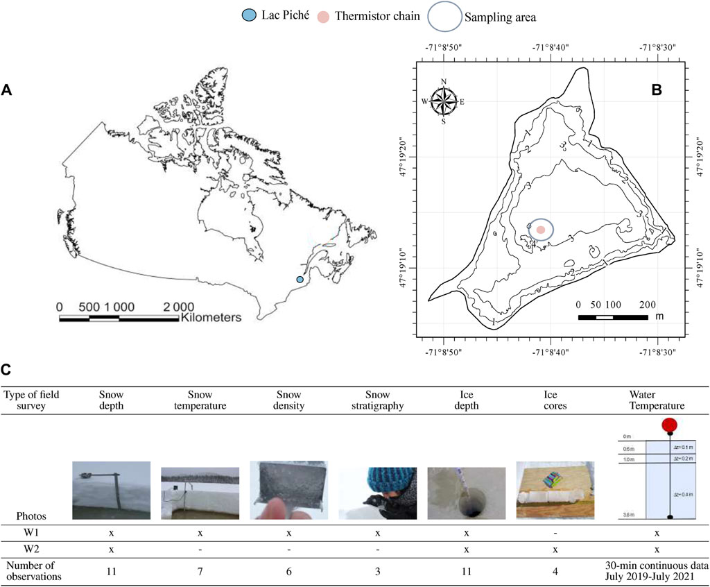
Figure 1. (A) Location of the study site in eastern Canada. (B) Bathymetric map of Lake Piché. The isolines present curves of equal depth, in meters. (C) Overview of sampling campaigns and experimental set-up.
Field monitoring was conducted over two consecutive winters, 2019-20 (W1) and 2020-21 (W2), as synthesized in Figure 1C. Water temperature measurements were collected continuously from July 2019 to July 2021. For this purpose, a vertical chain of thermistors probes (HOBO TidbiT v2, ±0.21°C accuracy from 0°C to 50°C) was installed in the deepest portion of the lake. Temperature measurements were taken from the surface to a depth of 3.8 m, with a vertical resolution of 0.1 m in the first 0.6 m, 0.2 m between 0.6 and 1 m, and 0.4 m between 1 and 3.8 m.
Occasional snow and ice surveys were carried out within a 10 m radius of the chain of thermistors. The measurement protocol varied from one winter to the next, as the site is not easily accessible at that time of the year. In the first winter, the total ice thickness was measured with an ice auger (model IMS-410-002, Kovacs). One snow pit per outing was also carried out. For each snow pit, a ruler was used to measure snow depth. Seven vertical temperature profiles within the snowpack were collected using a temperature probe (GTH 175 PT, Greisinger, ±1% accuracy) on 6 of 7 occasions the vertical density profile was also measured using a 100-cm3 Snow-Hydro box cutter, using a layer-based resolution varying between 2 and 4 cm. Crystal types, sizes, and shapes were identified using a magnifying lens and a millimetric grid. During the second winter of measurements, more detailed monitoring of the ice stratigraphy was carried out, thanks to a coring system (Mark II model, Kovacs). In this study, ice layers were visually identified on-site, but there was no examination under polarized light in a cold laboratory. A time-lapse camera (model HFP2Xm, Reconyx) was also installed onshore to monitor the freeze-up and break-up during the first winter. Unfortunately, these photos are only available for the first winter, as the camera was stolen before the end of the second winter. In the latter case, we use Sentinel-2 satellite images to determine freeze-up and break-up dates.
2.2 Model description
The CSLM is a finite difference, one-dimensional surface scheme model with a fixed vertical resolution. It has been developed to model the thermal structure of small freshwater lakes for weather and climate modelling applications (Mackay, 2012). The model is designed to simulate the physical processes taking place within the water column and the exchanges of energy, mass, and momentum between the lake and the atmosphere. These interactions are computed within a so-called “skin” layer at the lake surface, detailed in Mackay (2012). The energy of the skin layer E is expressed as:
with K* referring to net shortwave radiation, L* to net longwave radiation,
The extinction coefficient b varies according to the turbidity of water. Typically, these variations are accounted for by employing a summation of terms, as expressed in Eq. 2:
In Rayner (1980), the used approach involves categorizing solar flux into visible and infrared bands. In the presence of ice, values from Patterson and Hamblin (1988) are utilized. In this study, we adopt the specific values outlined in Table 1.
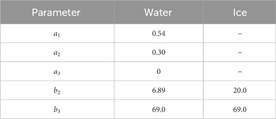
Table 1. Values of the coefficients in Eq. 3 as used in the CSLM, relating to the penetration of solar radiation into the water column.
The solar flux distribution within the water column is calculated, considering attenuation within each layer due to liquid or solid water, or a combination thereof, as applicable. In this current version of the CSLM, attenuation through snow cover is not incorporated. Subsequently, the conductive heat flux profile is determined through thermal conduction, where the flux F(z) is governed by the equation
The thermal properties of the sediment layer and the heat flux between water and sediment are other crucial lake processes. MacKay (2019) provides a detailed description of how they are included in the CSLM.
The snow physics module of the Canadian Land Surface Scheme (CLASS) model (Verseghy, 2012) is incorporated into CSLM, in addition to a dedicated snow-ice production scheme (Mackay et al., 2017), whose main processes are detailed below.
2.2.1 Snow-ice production scheme
In the CSLM (see Figure A1 in Mackay et al. (2017)), ice forms when the top layer cools slightly below 0°C, and the energy balance in Eq-1 becomes negative. The excess energy deficit is then used to freeze some surface water. Later, when snow falls on the ice cover, its weight may eventually exceed the carrying capacity of the ice, causing cracks in the cover that facilitate the upward migration of water, flooding part of the snow layer and forming slush (a mixture of snow-ice and liquid water). The water in the slush layer eventually freezes when exposed to subzero temperatures. Part of the latent heat released by the freezing water raises the temperature of the surrounding ice in the slush layer to 0°C. The remaining heat is transferred to the overlying snow, which warms up and may also undergo some melting. Eventually, the new layer of ice is thicker than the initial depth of the water-flooded snow because of the thermal expansion of the water as it freezes. When the energy balance is positive for an ice layer, the energy is used to raise the temperature of the ice to 0°C, and the remaining energy is used for melting.
Overall, the change in thickness Zi during the timestep Δt is governed by a complex interplay of factors, including temperature and water/ice depth, that determine the available energy, QM,w:
where Δt is the time step, ρi is the ice density, Lf is the latent heat of fusion, and QM,w is the heat exchange between ice and water is the heat associated with melting or freezing of water affecting the rate of ice formation and the thickness of the resulting ice layer, expressed as:
where Tfz is the temperature at freezing point.
2.2.2 Snow physics parameterization
The CSLM snowpack is modeled as a distinct layer on top of the ice, with its own characteristics, including thermal conductivity, heat capacity, and albedo. When the temperature of the snowpack reaches 0°C, the excess heat is applied to melting. The resulting meltwater (plus any liquid water from precipitation) percolates into the snowpack, shares its energy with the snow grain, and eventually refreezes if the pack is not already ripened to 0°C. The rate of melting and refreezing within the snowpack is also influenced by the temperature gradient within the snowpack, snow density and structure of the snow, and the presence of meltwater or rainfall (Verseghy, 2012; Mackay et al., 2017).
The temperature of the snow surface layer is estimated from the average snowpack temperature and the surface energy balance resolution. Net energy and moisture fluxes are calculated at the end of each time step:
where QM,s is the heat associated with the melting or freezing of water and QI,s is the changes in heat storage due to the phase change of snowpack.
Then, in the CSLM, the change in temperature of the snowpack ΔTs is expressed by:
where Xs is the fractional coverage of the snowpack, Cs is the heat capacity of the snowpack, and t is the current time step. Some of the key physical characteristics of snow for this study are described in the following paragraphs.
2.2.2.1 Thickness
In the CSLM, snow thickness (zs) is a function of snow mass (Ms) and snow density, (ρs) expressed by:
2.2.2.2 Heat capacity
In CSLM, the heat capacity of the snowpack (Cs) is computed as:
where Ci and Cw are heat capacities (J m−3 K−1) of ice and water, ρs, ρi, and ρw are densities (kg m−3) of the snow, ice and water, ws is the water content (kg m−2)and zs is the depth of the snowpack (m).
2.2.2.3 Fractional coverage
The fractional snow coverage Xs refers to the spatial extent of the snow cover (Verseghy, 2012). Mass conservation is applied to estimate the fractional snow cover when the calculated snow depth is less than a threshold value. Therefore, a limiting snow depth zs,Lim is required for an area to be considered snow-covered, and the fractional snow coverage Xs is then calculated by dividing the mass of snow in the area by the mass of snow that would be present if the snow depth were equal to the threshold value:
To accurately estimate the snow water equivalent (SWE), it is important to adjust the water content of the snowpack accordingly by accounting for the fractional area of new snow. In fact, when new snow falls on an existing snowpack, it potentially alters the density and water content.
2.2.2.4 Albedo
The albedo refers to the fraction of incoming shortwave radiation that is reflected by the surface of the snow. In the CSLM, the total snow albedo αs decreases according to the following empirical exponential decay function:
where t is the current time step. According to Aguado (1985); Robinson and Kukla (1984) and Dirmhirn and Eaton (1975), typical total snow albedos from visible and near-IR components for fresh snow, old dry snow, and melting snow are used (total fresh snow equal to 0.84, and total melting snow equal to 0.50).
2.2.2.5 Density
The density of fresh snow
2.3 Meteorological inputs
The CSLM model requires seven meteorological inputs. Most of these were collected at the nearest federal weather station (RCS), some 0.5 km from the lake. The radiation data were collected from the Sapling flux tower (Isabelle et al., 2020a), 4 km to the south (Figures 2A,B).
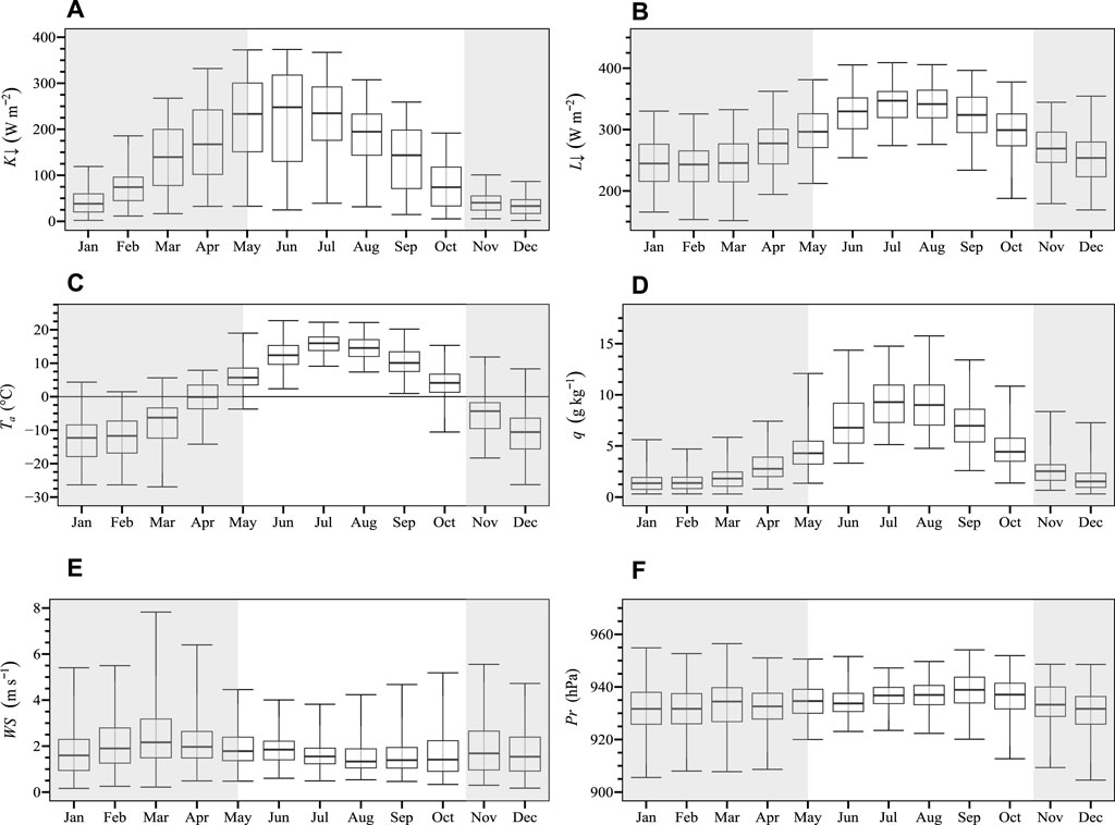
Figure 2. Monthly pattern of the daily meteorological forcing from 01 January 2017 to 31 October 2021 differentiating open water (white) and ice cover periods (gray): (A) incoming shortwave radiation (K ↓), (B) incoming longwave radiation (L ↓), (C) air temperature (Ta), (D) specific humidity (q), (E) wind speed (WS), and (F) atmospheric pressure (Pr). Whiskers extend to the minimum and maximum values, and boxes show the interquartile range.
The monthly mean of the incoming shortwave radiation reaches 375 W m−2 in summer but falls to 100 W m−2 in winter. Incoming longwave radiation oscillates between 180 and 400 W m−2. Near-surface air temperature follows a seasonal pattern, with negative values during the ice cover period (November-April), and reaching 25°C during the open-water period (May-October). Winter is slightly windier than the rest of the year, with low specific humidity values never exceeding 5 g kg−1 owing to the very cold temperatures.
Total precipitation measured at the RCS federal weather station is split into liquid and solid precipitation by employing near-surface air temperature observations at each time step. When above 2°C, total precipitation is assumed to be liquid, while it is considered solid if it occurs in the presence of air temperature less than or equal to 0°C. A linear partitioning of liquid-solid precipitation between 0°C and 2°C is applied. The prevalence of each precipitation phase on a monthly scale is illustrated in Figure 3.
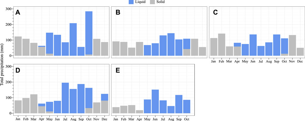
Figure 3. Monthly accumulated total precipitation: (A) year 2017, (B) year 2018, (C) year 2019, (D) year 2020, and (E) year 2021. Blue bars are liquid precipitation, and gray bars, solid precipitation (water equivalent).
2.4 Model parametrization
Table 2 presents selected parameters and their assigned values. The CSLM model, driven in its standalone mode, is run with 30-min time steps. Observations were used to guide some of the value selections. Lake depth was fixed at 3 m over 10 m of sediments (default value), values leading to the best performance in reproducing water temperatures using a vertical resolution of 0.1 m. The lake fetch was fixed to 385 m, corresponding to the root square of the lake area (≈0.15 km2). Since the lake is small and surrounded by terrestrial landscape, the wind sheltering factor was fixed to 0.3 meaning that the surface drag coefficient was reduced by 70%. An initial neutral temperature profile was imposed for the first day of the simulation. The simulation period extends from 1 January 2017 to 31 October 2021, with 2 years of spin-up; the control (sampling) period from 25 October 2019 to 20 July 2021. An extinction coefficient of 0.7 m−1 was concluded from Beer’s law and measured using a Secchi disk.
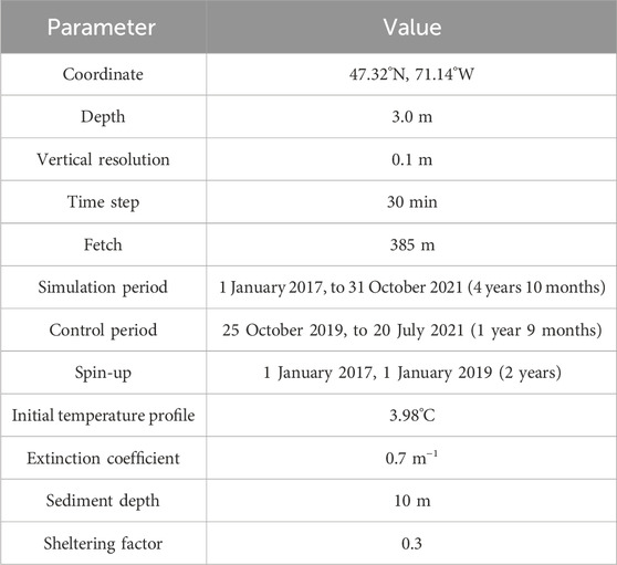
Table 2. CSLM parametrization.
3 Results
3.1 Snow and ice properties
3.1.1 Ice and snow thicknesses
The CSLM total ice thickness (clear ice + snow ice) shows a good agreement with observations (Figures 4A) with a moderate overestimation (between 1% and 40%). It is important to note that snow ice production begins when the snow weight exceeds the carrying capacity of the ice. In W1, snow-ice production begins 1 day after the freeze-up date, while in W2, it starts 6 days after the ice cover is installed, allowing a more substantial layer of clear ice to form, and during this time clear ice forms the entire ice layer.
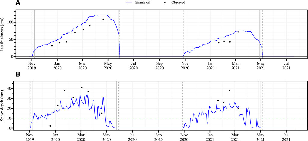
Figure 4. Observed (black dots) and simulated (blue line) snow depth over Lake Piché. (A) Ice thickness. Dashed gray lines show the simulated freeze-up and breakup dates. (B) Snow depth. The green dashed line illustrates the snow height below which the snowpack becomes patchy (Zs,lim = 10 cm).
In the first winter, freeze-up occurred in early November, while in the second, it occurred in late October. The simulated ice layer reached a maximum thickness of 121 cm in W1 and 75 cm in W2, which is slightly overestimated compared to observations, which show a maximum thickness of 109 cm in W1 and 72 cm in W2. Both observed and simulated maxima are consistent with the fact that the second winter was on average 3°C warmer than the first one (average temperature −4°C vs. −7°C). In both winters, ice growth was spread over several months (5 in 2021, 4 in 2020), while melting took 1-month on average. We also note a larger mean bias during W1 (+15 cm) than W2 (+12 cm).
In both winters, a thin snow cover of 2–41 cm accumulated over the ice over the entire season (Figure 4B). In the model, the snowpack is assumed to fully cover the ice when its thickness exceeds 10 cm (green dashed line in Figure 4B), below which the snowpack becomes patchy (the depth is then held constant at 10 cm, and the snow cover is recalculated based on conservation of mass). For a more meaningful comparison between the modeled and observed snow thickness, modeled values were multiplied by the snow fraction to provide a more accurate representation of the snowpack inside a grid cell. The maximum simulated snow depth reached 35 cm in March 2020, while the observed depth was between 37 and 41 cm during the same period. Overall, snow heights show a reasonably good agreement with a slight underestimation compared to observations (mean bias of −5 cm), given the spatial heterogeneity of snow heights resulting from wind transport and given the relative simplicity of the CSLM snow module, which is single-layered.
A comparison between the simulated and observed (Figure 5) freeze-up and break-up dates is given in Table 3. The simulated ice freeze-up occurs 5 days (W1) and 6 days (W2) earlier than observed for both winters. In comparison, the simulated ice breakup is delayed by 4 (W1) and 8 (W2) days. This leads to overall errors in the ice cover duration that never exceed 14 days, suggesting a reasonably accurate performance of the CSLM. In determining freeze-up and break-up dates from Sentinel-2 satellite imagery in W2, we used the first cloud-free date when the lake is completely ice-covered or uncovered. For the winter of 2020–21, the images suggest partial ice cover on 10 October 2020, and breakup beginning on 15 April 2021, introducing uncertainties in our estimates of up to 19 days of ice duration.
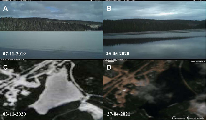
Figure 5. Observed dates are collected from the on-shore camera in W1 (A, B) and Sentinel-2 satellite images in W2 (C, D).
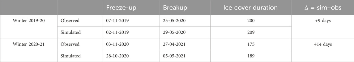
Table 3. Observed and modelled dates of freeze-up and break-up.
The observed ice cores during W2 are compared with the CSLM simulations in Figure 6. Ice cores showed multiple alternating layers of clear ice, slush, and snow ice. To address the lack of a slush scheme in the CSLM, we define snow ice thickness as the combined thickness of slush and snow ice. On 21 January 2021, the snow ice thickness was overestimated by approximately 8 cm. Additionally, there were 31 cm of observed clear ice and 35 cm of simulated clear ice, resulting in an overestimation of 11 cm for the total ice. On 03 February 2021, the snow-ice thickness was overestimated by about 2 cm, with 18 cm observed and 20 cm simulated. Between 21 January 2021 and 03 February 2021, both observed and simulated snow ice became thicker. Clear ice thickness was 27 cm (observed) and 37 cm (simulated). Noting a rise in air temperature during this period, this may have led to the formation of slush, which then converted, since there is no scheme for slush in the model, to snow ice. On 17 February 2021, there was an increase in clear ice by 6 cm (observed) and by 4 cm (simulated) and the snow ice became thinner. The current conditions are cold, and the ice is snow-covered, suggesting a transition from snow ice to clear ice. On 10 March 2021, both the observed and simulated snow ice became thicker. The model is generating excessive snow ice, leading to excessive total ice and insufficient snow cover. As shown in Figure 4 and Figure 6, on 10 March 2021, while the lake model accurately simulates the total ice thickness (bias of 2 cm) and the snow depth (bias of −1 cm), it shows discrepancies with observations in modeling individual ice types. The model underestimated the clear ice by 11 cm (−24%) and overestimated the snow ice thickness by 14 cm (+49%).
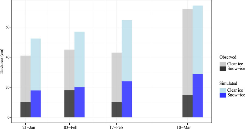
Figure 6. Observed (black) and simulated (dark blue) snow-ice; and observed (gray) and simulated (light blue) clear ice during W2 (year 2021).
3.1.2 Snow density and temperature
A comparison of observed and CSLM-simulated snow cover properties is illustrated in Figure 7. Overall, we find that the CSLM model performs better in simulating snowpack temperatures (Figure 7A, mean Pearson correlation coefficient (r) of 0.90, p − value < 10–2) than in simulating snowpack density (Figure 7B, r = 0.10, p − value = 0.9).
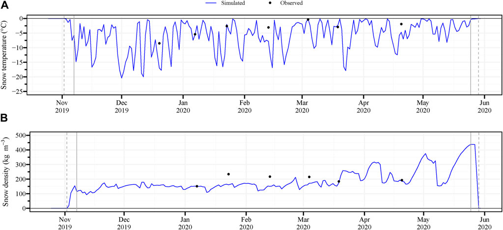
Figure 7. Daily observed (points) and CSLM simulated (blue line): (A) snow temperature, and (B) snow density during the control period. Measurements were made only during W1. Solid (observed) and dashed (simulated) gray lines show the freeze-up and breakup dates. Observations were averaged over the total snow depth.
In general, the model performs well in capturing the overall trends in snow temperature, albeit with a slight tendency towards an underestimation (mean bias of −2°C). For example, during 4 measurements (23 January 2020, 04 March 2020, 19 March 2020), the model shows a more satisfactory performance with a slight overestimation of 0.4°C, while a mean cold bias of 4°C is observed during the remaining measurement days. In fact, if the snow height is inaccurately modeled (underestimated by 5 cm in this case), it is challenging for the model to simulate the snow temperature properly due to the inaccurate representation of snow enthalpy. Besides, the maximum error in snow temperature estimate was observed on 19 December 2019 (a cold bias of 8.5°C), and when we look closer at snow depth on the same date, we can also note an overestimation of 11 cm in simulated snow depths which is the highest snow depth error also. This could be due to the fact that the observed snow cover (Zs = 2.4 cm) is below the threshold and so the model does not take into account snow ablation processes.
Observed and CSLM simulated snow density is also shown in Figure 7B. The density could not be measured on 19 December 2019 because the snow layer was too thin (2.4 cm). The model generally underestimates density, with a mean bias of −34 kg m−3. Since there is a positive correlation between snow density and snow depth, the underestimation of snow density could be explained by the underestimation of snow depth. Snow density also affects pore spaces available to liquid water and the melting rate. As more snow accumulates on top of the snowpack, the layers beneath experience increasing pressure, reducing airspace between snow particles and the overall densification of the snowpack. Then, an underestimation of snow density can be explained by a more porous snow and then an overestimated liquid water, which causes the overestimation of the snow ice layer.
3.2 Water temperature
Figure 8 compares the timing of each limnological period on the observed and simulated lake. The cooling period for the model and observations in W2 (Figure 8B) lasts for a maximum of 3 weeks. The fall overturn happens up to 8 days (observations) and up to 2 days (simulations) before the freeze-up. However, the model underestimates fall overturns in both years (1 day for year 1 and 2 days for year 2) as well as the cooling period during year 2 by 9 days. This suggests that the model cools down the simulated lake quickly, resulting in an early freeze-up (e.g., 5 days in advance in W1 and 6 days in advance in W2). In terms of the pre-melting period, the heating period is slower in the simulation (12 days in W1 and 20 days in W2) compared to the observations (4 days in W1 and 12 days in W2). As a result, the simulated water temperature takes longer to rise. This could explain the delayed break-up dates in the simulation for both winters (4 days in W1 and 8 days in W2). Within 1 day after the ice-off, the spring turnovers occur for observations and simulations. Finally, summer stratification duration is well simulated with an error of 1 day in year 1 (no available data for year 2). Accordingly, the model is less performant in reproducing the dimictic thermal pattern of the observed lake, and its shallowness makes it very responsive to air temperature fluctuations and wind mixing leading to a polymictic lake.
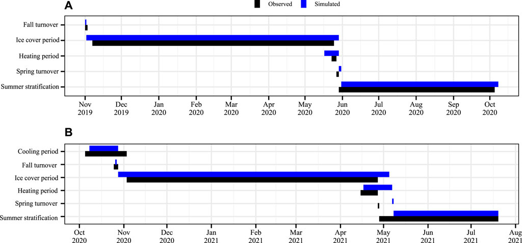
Figure 8. Timing and duration of observed (black bars) and simulated (blue bars) limnological period for (A) W1 (B) W2.
Figure 9 illustrates the evolution of the simulated and observed water temperatures. The simulated temperature profile reveals that the reproduction of the vertical layering of the water column following a seasonal pattern is close to observations. However, the simulated lake remains at the freezing temperature throughout its depth, and winter inverse stratification is not well reproduced (particularly in W2). It is known that thermal mixing is generally induced by both free and forced convection, including wind and buoyancy mixing (only free convection prevails in the ice-cover period). The discrepancy may be explained by the fact that free convection is not adequate to mix the underlying water. Moreover, this is also due to the overestimation of simulated ice thickness, leading to less light penetration. The performance of the model in simulating water temperature differs with depth, indicating errors in both directions (e.g., an overestimation of open-water temperatures and an underestimation of ice-cover temperatures). Therefore, the mean absolute error (MAE) is a more likely interpretable metric in studying the model performance along the control period. The model shows better abilities to simulate temperature at the surface (within the first 0.5 m) with a MAE of 0.6°C and the metalimnion layer (MAE = 0.8°C) compared to hypolimnion (MAE = 1.5°C).
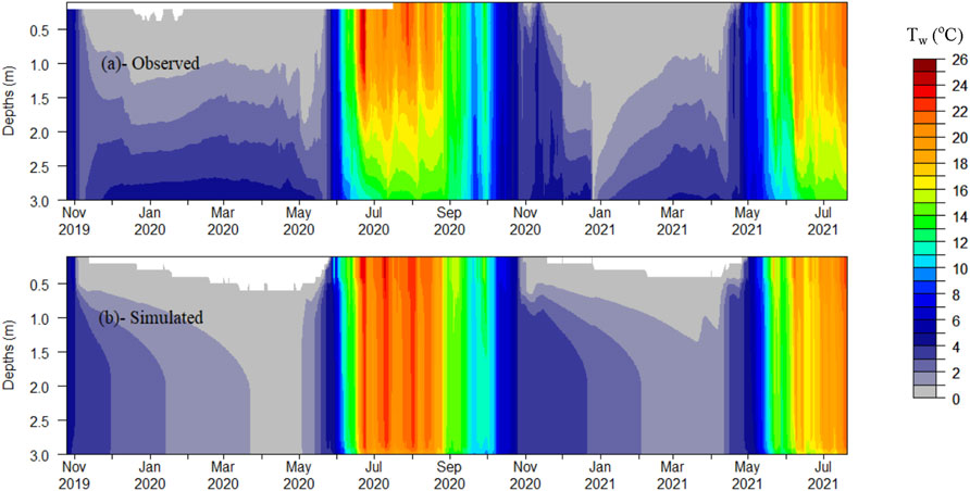
Figure 9. Temperature profiles during the control period: (A) observed and (B) simulated daily water temperatures.
Finally, in Figure 10, the analysis of the model mean bias for the ice cover period and open water periods demonstrates a more accentuated discrepancy during the ice cover periods. In the open water period, the model reproduces better the water temperature with warm biases of 0.9°C at the surface and 1.0°C at 1 m depth, while deep waters have a warm bias of 2.8°C. This could be explained by a greater vertical mixing which leads to warmer water temperatures at the lake bottom, which could also be caused by an overreaction of the model to high wind events (Kallel et al., 2023). On the other hand, in the presence of an ice cover, water temperature is underestimated with mean cold biases of 0.6°C at the surface (0.5-m depth) and 1.3°C in deep waters. This means the simulated stored heat in the deep water column is not sufficient to reproduce winter inverse stratification. Overall, the model is more accurate in reproducing surface temperatures rather than the lake bottom temperatures.
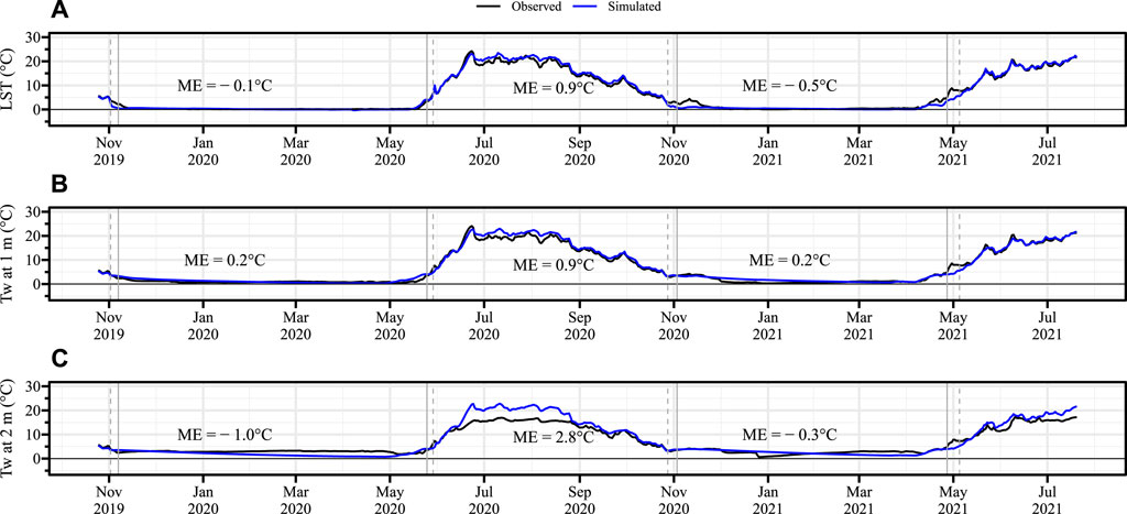
Figure 10. Time series of water temperature at: (A)- 0.5 m (LST), (B)- 1 m, and (C)- 2 m. Dashed gray lines show the simulated ice-on and ice-off dates. Mean errors (ME) are also presented for each period.
4 Discussion
4.1 Snow model performance
The CSLM exhibited relatively good agreement with observed snow heights, with a mean bias of −5 cm. The highest error in snow estimate is noted on 19 December 2019 (overestimation of +11 cm) when the observed snow cover (Zs = 2.4 cm) is below the threshold (
As shown in Figures 4B, 7, there is a discrepancy in snow height, temperature, and density between the observations and the CSLM. This could be partly explained by the absence in the model of some key snow processes that drive the development of snowpacks on lake ice. Figure 11 illustrates the complexity of the snowpack vertical profile observed on 23 January 2020. A seasonal snowpack undergoes continuous metamorphism caused by environmental conditions such as air temperature fluctuations, solid and liquid precipitation events, short- and longwave radiation, and wind (Sommerfeld and LaChapelle, 1970). This leads to the formation of different snow layers (Figure 11A). For instance, air temperature fluctuations lead to the non-uniform vertical snow temperature profile in Figure 11B. A strong vertical temperature gradient is known to trigger upward water vapor fluxes that create faceted crystals or depth hoar, as observed at the bottom half of the snowpack (Colbeck, 1983). For their part, winter rain-on-snow (ROS) events lead to the formation of ice layers, as in Figures 11A, E, F). Such a phenomenon densifies the snowpack locally (Figure 11C) and increases the average density of the snowpack. Snowpack densification could also originate from wind that breaks and redistributes snow particles at the snow surface (Pomeroy and Gray, 1990). A single-layer snow model, as implemented in CLSM, is unable to simulate these processes and to reproduce accurately the high level of complexity of the snowpack as one could observe. However, an aged-based snow densification function in a single-layer snow model provides the general behavior of a densifying snowpack at a low cost. Overall, the vertical complexity of the actual snowpack properties should be considered when using this simple, but rather coarse, snow modeling approach.
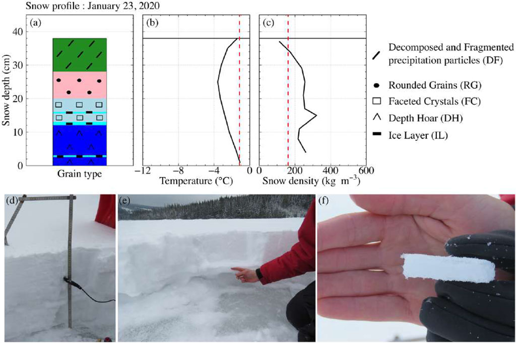
Figure 11. Snow profile from 23 January 2020. The snowpack stratigraphy is shown in frame (A) with the color code according to Fierz et al. (2009). The vertical profiles of snow temperature and density are shown in frames (B) and (C). The dashed red line indicates the temperature and density of the simulated snowpack on this date. The frame (D) shows a photo of the snow pit wall during a temperature measurement. The frame (E) shows the two successive ice layers in the middle part of the snowpack, distanced by a few centimeters. Finally, in frame (F), we present a photo of the 1.5 cm thick ice layer at a depth of 12 cm.
4.1.1 Sensitivity analysis of sheltering reduction factor
In (sub)arctic environments, wind plays an important role in the freeze-up and breakup of lake ice, as well as the redistribution of snow, significantly influencing the overall dynamics of these ecosystems. Wind sheltering, a phenomenon wherein nearby land features or vegetation reduce the impact of wind on water surfaces, has been extensively studied (Vickers and Mahrt, 1997; Venäläinen et al., 1998; MacKay, 2019). The CSLM incorporates sheltering effects through a sheltering reduction factor, modifying the drag coefficient to account for the surface friction reduction as follows (MacKay, 2019):
Where Ua is the wind speed, CD is the drag coefficient, and S is a sheltering coefficient ranging between 0 and 1.
The absence of sheltering, as represented in CSLM through a sheltering reduction factor of 1, signifies an environment where wind interacts directly with the lake surface, devoid of any drag reduction typically provided by vegetation or topographical features. This scenario is characteristic of tundra-like environments with sparse vegetation and limited sheltering. Such conditions have significant implications for ice and snow dynamics within these ecosystems. Notably, the effect of fetch on surface stress and drag coefficient varies with model parameters and lake characteristics. For smaller boreal lakes like Piché Lake, surrounded by forest, these nuances are particularly relevant. Therefore, a detailed comparison of the model’s performance in reproducing ice freeze-up and breakup, snow cover, and water temperature is conducted to assess the effects of wind sheltering. For instance, in cases where sheltering is not considered, CSLM simulates a snow cover of 17 cm on 13 February 2020, while observations show it to be 25 cm. Similarly, in Figure 12 we note that the modeled bottom temperatures exhibit higher discrepancies from observations when sheltering is not considered (MAE(without sheltering)= 2.2°C vs. MAE(with sheltering)= 1.5°C). However, differences in modeling ice thickness and duration are not significant between the two tests.
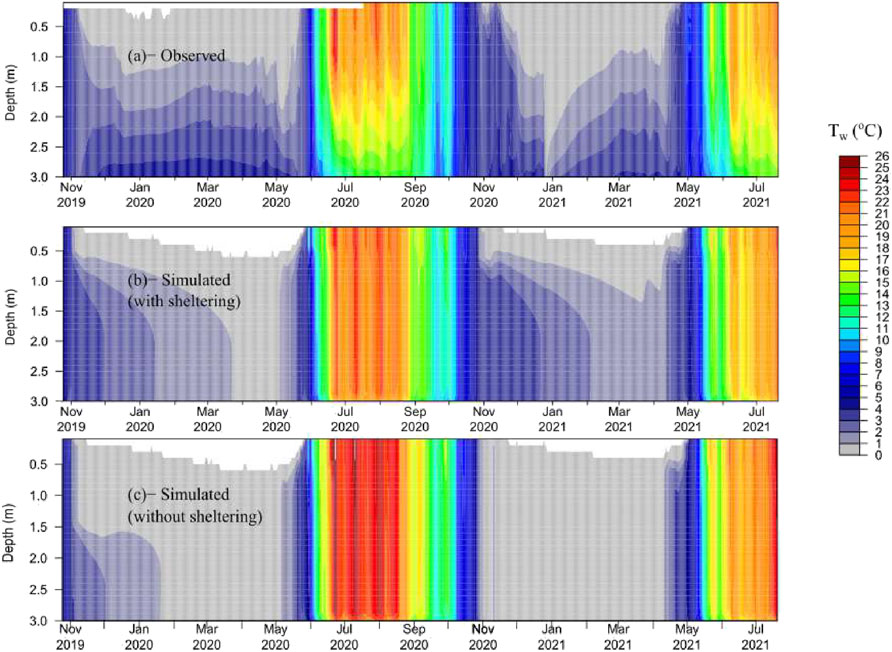
Figure 12. Temperature profiles during the control period: (A) observed, (B) simulated (with S = 0.3) and (C) simulated (with S = 1) daily water temperatures.
4.2 CSLM performance
Table 4 provides a comparison between the current research and the study conducted by Mackay et al. (2017). Both studies’ main objective is the validation of CSLM during the ice season on a shallow boreal lake. Each study has its own advantages and limitations. One of the original features of our study comes from the time series of ice and snow measurements conducted throughout the winter season, providing a more comprehensive understanding of the ice and snow dynamics. Furthermore, the present study involved a total of 11 measurements of snow depth, offering a more extensive dataset compared to the single measurement carried out by Mackay et al. (2017). Through extensive fieldwork and data collection, we were able to improve the model parameters to better match real-world conditions (lake bathymetry, sheltering reduction factor, penetrating light). In contrast, Mackay et al. (2017) relied on past observations to validate the model (e.g., meteorological conditions to determine ice freeze-up and break-up dates, minimum/maximum and mean past data of ice, ice-snow, snow thicknesses). In addition, the differences in climatology between the two study sites make it possible to explore contrasting operating conditions for the model. Our research explores a study site characterized by colder temperatures, greater snowfall, and earlier freeze-up compared to the warmer climate of the Experimental Lakes Area in northwestern Ontario, as studied by Mackay et al. (2017).
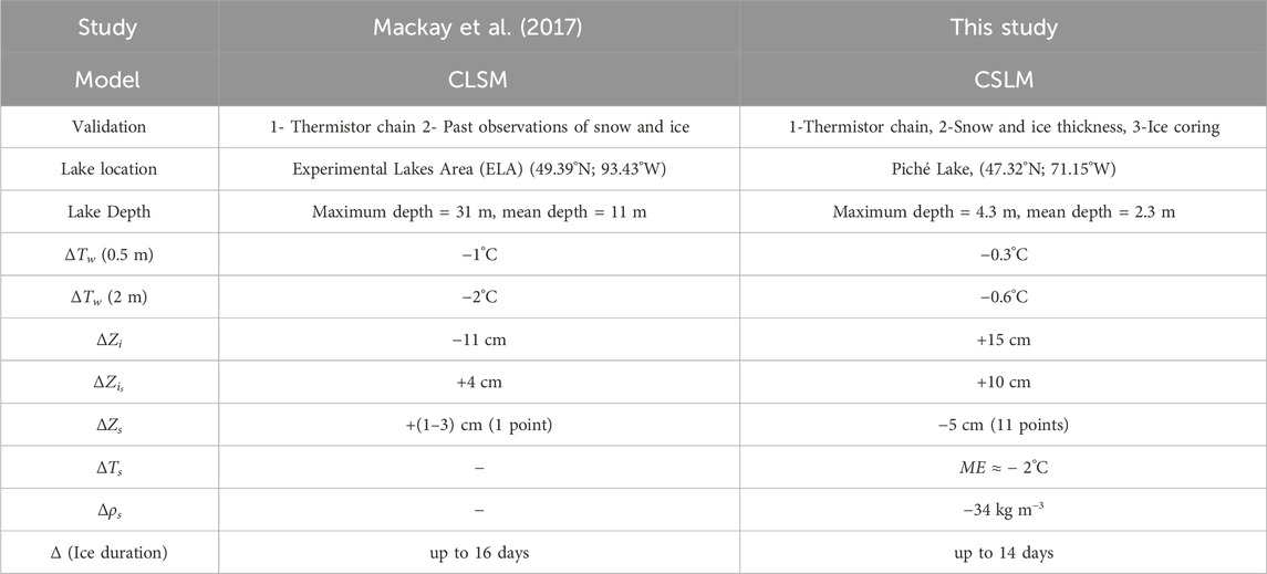
Table 4. Comparison of studies of ice-season CSLM validation on a shallow and boreal lake; Δ refers to the bias between simulation and observation of water temperature during the two ice-cover periods (Tw) at the 0.5 m and at 2 m, the mean total ice thickness (Zi; clear + snow-ice), the snow-ice thickness
Another contrasting aspect is the consideration of spatial variability within the lake. Mackay et al. (2017) accounted for this by sampling different locations, whereas this study did not. This could affect snow depth estimation (snow was underestimated, leading to an underestimation of its density). Validation of precipitation inputs is a crucial step toward successful snow modeling. Same as Mackay et al. (2017), this study did undertake precipitation validation by correcting the wind-induced oscillations and the under-catch bias in the precipitation measurements from Geonor precipitation gauge.
Ice cover duration is well simulated when compared to observations (camera and Sentinel-2 satellite images) in this study, with an error of 9 and 14 days. Mackay et al. (2017) found errors up to 16 days. The timing of ice-on is generally slightly too early in CSLM, which aligns with the findings from Mackay et al. (2017). The slight discrepancy between the simulated and observed ice freeze-up and breakup can be attributed to several factors. One possible explanation is that the early ice freeze-up can be caused by a more rapid drop in simulated water temperatures. Moreover, the one-dimensionality of the model can lead to limitations in capturing the full complexity of ice heterogeneity. Likewise, if the simulated ice thickness is overestimated, a slower heat transfer rate between the lake and the atmosphere could occur, resulting in a delayed ice breakup.
The model demonstrated a reasonably accurate representation of the total ice thickness during the control period, with a mean bias of 15 cm. These results revealed that the CSLM generally captured the trend of ice growth, although some differences were observed between the observed and simulated ice growth rates. During the analyzed period, the mean ice growth rates in W1 were 0.6 cm day−1 for observations and 0.7 cm day−1 for simulations, while in W2, both observed and simulated ice growth rates were about 0.5 cm day−1 for observations and simulations. It is worth noting that there were instances where the simulated and observed ice growth rates aligned reasonably well. However, when examining individual layers, there were differences between the simulated and observed, with an overestimation of the snow-ice growth rate (mean growth rate of −0.1 cm day−1 for observations and 0.3 cm day−1 for simulations) and an underestimation of clear ice (mean growth rate of 0.4 cm day−1 for observations and 0.08 cm day−1 for simulations).
The formation of a slush layer within the snowpack is caused by flooding of the snow layer with liquid water (Mackay et al., 2017). Knowing that there is no slush scheme in the CSLM and once the slush is formed, it is directly converted to snow ice or drained off. Then, the overestimation of the snow ice layer and the underestimation of the snow layer point toward an underestimation of the ice capacity factor. Indeed, the amount of liquid water in the slush layer is limited by the pore volume within the snow. However, CSLM assumes a complete pore saturation, which could potentially introduce errors in estimating the flooded layer and, consequently, the snow ice layer. Also, knowing that freezing of liquid water releases latent heat, the snow in the slush layer warms to 0°C, with the remaining heat assigned to the overlying snow, causing snow melting. Consequently, an overestimation of the snow ice layer can lead to an overestimation of the warming heat and, subsequently, an underestimation of the snow due to the slush thermal expansion. It is also important to consider the uncertainties associated with the field measurements in the reference dataset.
In both studies, the surface water temperature was well simulated; however, deep layer temperatures were underestimated. It is also hypothesized that mixing was not sufficient for the heat to reach the bottom of the lake. We considered a slab thickness of 10 m and a pure sand layer. Thermal properties were taken from MacKay (2019). This allowed a slight improvement of deep layer temperature (MAE (no sediment) = 3°C vs. MAE (with sediments) = 1.5°C). The simulated fall turnover and the cooling duration are underestimated, while the lake is ice-covered before the observations. This can be attributed to the rapid drop in simulated water temperatures, prompting ice formation. Additionally, strong fall winds induce vertical mixing throughout the lake depth. Results showed that the model overestimates vertical mixing. Furthermore, CSLM underestimates the ice thickness by 15 cm during the entire control period, resulting in an increased light penetration and earlier lake heating compared to observations. Specifically, in W2, the heating phase begins approximately 7 days earlier in the simulation. These findings suggest that the CSLM may need further improvements in accurately capturing the timing and dynamics of fall turnover and the subsequent freeze-up and break-up process. When modeling ice thickness, it is crucial to accurately represent this parameter, as it directly influences the penetration of light through the ice cover, subsequently influencing the available energy in the water column. Notably, during the ice-off period of 2021, Figure 9 illustrates a deviation of the modeled thermal structure from observations by mid-April, indicating that the water column is already well-mixed and restratifying. A closer examination during this period (Figure 13) reveals that the simulated breakup occurs on 5 May 2021, which is 8 days later than observed (on 28 April 2021), coinciding with the complete melting of the snow cover. Simultaneously, shortwave radiation penetrates the ice, creating a layer of gravitational instability that gradually expands across the entire column. It is evident that further refinement of the ice ablation/ice-off period may be necessary in the model to accurately simulate the springtime thermal structure.
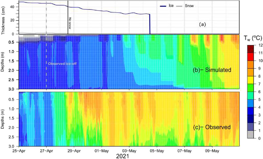
Figure 13. Simulated snow (gray) and ice (blue) thicknesses (A), and simulated (B) and observed (C) temperature profiles during the spring stratification 2021.
5 Conclusion
The objective of this project was to evaluate the performance of the Canadian Small Lake Model (CSLM) in simulating the thermal dynamics, ice cover, and snowpack of a shallow boreal lake: Lake Piché. The original contribution of this study lies in the use of field measurements encompassing water temperature, snowpack properties (height, density, and temperature), ice thickness, and lake characteristics (light extinction and depth) to evaluate the lake model.The following key findings have been identified:
1. Observations and simulations aligned in terms of reaching maximum snow heights during both winters. While the simulations approximated the observed values, a minor underestimation in snow height was observed.
2. The CSLM underestimates the snow density by 34 kg m−3 on average. This implies a more porous simulated snowpack, which favors an overestimation of available liquid water and consequently an overestimation of snow ice. Additionally, the model slightly underestimates snow temperature. The snow model single-layer assumption plays a significant role in these discrepancies. By assuming uniform properties throughout the entire snowpack, including density, temperature, and moisture content, the CSLM disregards the vertical variations. This limitation affects the CSLM performance to capture the complex interplay of snow processes, such as snow metamorphism, layering, and vertical temperature gradients.
3. CSLM accurately simulates ice thickness, with an overall overestimation of 15 cm. Particularly, a high level of agreement between observed and simulated maximum total ice thickness was found. This suggests that the model adeptly captures variations in ice thickness, demonstrating the model performance in representing ice dynamics.
4. Simulated freeze-up occurs 5 days too early in W1 and 6 days too early in W2. The analysis shows an underestimation of the duration of the autumn overturn, which implies that the CSLM cools the water faster than in reality. As for the simulated breakup, it occurs 4 days too late in W1 and 8 days too late in W2. The overestimation of the heating periods by 8 days in both winters may contribute to delays in the ice breakup, as the water temperature in the model takes longer to rise.
5. Examination of the ice cores reveals a key finding. While the total ice thickness shows a close agreement between simulation and observation (mean bias of 2 cm), clear ice is underestimated by 11 cm, and snow ice is overestimated by 14 cm in the simulation. The model performs better in simulating clear ice than snow ice, possibly due to factors such as an underestimated ice-carrying capacity. Moreover, the overestimation of snow ice may be due to the assumption of a complete pore saturation, resulting in an overestimation of the flooded layer. One potential improvement could be to decrease the efficiency of snow ice production.
6. The CSLM correctly reproduces the summer stratification of the lake, with a better agreement for surface temperature (mean average error of 0.9°C) than for bottom temperature (mean average error of 2.8°C). Furthermore, during the ice cover period, the model exhibits a good accuracy in simulating the winter inverse stratification with slight discrepancies probably due to an overreaction to strong winds and an overestimation of the ice layer acting as a barrier to light penetration.
In conclusion, this study provides valuable insights into the performance of the CSLM in simulating the thermal regime, ice cover, and snowpack of a small boreal lake. The observed discrepancies highlight potential areas for model improvement, such as snow-ice formation processes. The introduction of a more sophisticated snowpack model that includes multiple layers and all metamorphism processes could lead to a more accurate representation of snow properties and their impact on lake dynamics. The implications of an accurate representation of lake ice cover affect a wide variety of environmental sciences. In biology, for example, we know that longer ice cover leads to reduced mixing during the stratification period, which affects nutrient cycling and oxygen levels in the water column. An accurate representation of these processes is therefore necessary to assess the effects of climate change on aquatic ecosystems. On the other hand, in large-scale climate modeling, the representation of ice cover longevity is crucial to reproduce surface albedos, which are highly contrasted during periods of open water and ice cover. Other applications (ice transport, limnology, hydrology) also reinforce the importance of this issue.
6 Snow stratigraphy
Snow grains refer to the individual snow crystals that make up the snowpack. These grains vary in shape, size, and density, which can have a significant impact on the stability of the snowpack and snow metamorphic processes (Leppäranta, 2015).
Snow layers (Supplementary Figure S1) were classified based on their physical properties and how they were formed following the methods in Fierz et al. (2009); Jacobi et al. (2019); Lehning et al. (2002). Here are different observed classes of snow stratigraphy:
1. New snow: freshly fallen snow that has not been affected by wind or other weather elements. It is often light and fluffy (Lehning et al., 2002).
2. Decomposing and fragmented precipitation particles: snow crystals that have been broken or fragmented by wind or temperature changes. They are dry and generally observed near the surface (Fierz et al., 2009).
3. Rounded grains: smooth, round grains that are created when snow crystals melt and refreeze. They are generally strong and stable (Fierz et al., 2009).
4. Faceted grains: flat and angular crystals that are often weak and increase avalanche risk. They are formed under very cold and dry conditions (Fierz et al., 2009).
5. Depth hoar: faceted grain that forms in the lower layers of the snowpack, from water vapor moving upwards and refreezing in the snowpack, creating large, weak, and loose crystals (Leppäranta, 2015).
6. Melt-freeze snow: particles that have gone through multiple freeze-thaw cycles, causing it to become denser and more compact. They are often found in areas with direct sun exposure (Leppäranta, 2015).
7 Ice stratigraphy
A classification of ice structure has been presented in Michel (1978). Three basic crystal structures exist (Supplementary Figure S2).
1. Primary Ice (Frazil frozen slush) forms as the first ice layer on the lake surface (Leppäranta, 2015). In laminar flow conditions, nucleation occurs when ice crystals form on suspended particles at the surface. This layer of ice is very thin and may be easily lost through melting or sublimation. Primary ice can also form on snow or ice nuclei precipitating onto the water surface.
2. Superimposed ice (Snow-ice) forms when liquid water or slush freezes on top of the primary ice. The formation of superimposed ice occurs in winter after the intrusion of lake water over the primary ice, or in spring during the nighttime cooling after the melting of snow or ice during the day due to solar radiation or warm temperatures (Leppäranta, 2015).
3. Secondary Ice (clear ice) forms beneath the primary ice layer. As it grows thicker, it insulates the water below from the cold air above. Initially, the insulation is not fully effective, and the temperature of the water below continues to drop, encouraging the expansion of the secondary ice layer.
Data availability statement
The original contributions presented in the study are included in the article/Supplementary material, further inquiries can be directed to the corresponding author.
Author contributions
HK: Conceptualization, Data curation, Formal Analysis, Investigation, Methodology, Resources, Validation, Visualization, Writing–original draft, Writing–review and editing. DN: Funding acquisition, Project administration, Resources, Supervision, Validation, Visualization, Writing–review and editing. BB: Formal Analysis, Investigation, Writing–review and editing. AT: Software, Writing–review and editing. MM: Writing–review and editing. FA: Funding acquisition, Project administration, Resources, Supervision, Validation, Visualization, Writing–review and editing, Formal Analysis, Methodology.
Funding
The author(s) declare financial support was received for the research, authorship, and/or publication of this article. This work was funded by Hydro-Québec and the Natural Sciences and Engineering Research Council of Canada (NSERC) through grant RDCCPJ508080-15, “Observation and modelling of net evaporation from a boreal hydroelectric reservoir complex (water footprint)”.
Acknowledgments
The authors would like to thank all those who supported the field work.
Conflict of interest
The authors declare that the research was conducted in the absence of any commercial or financial relationships that could be construed as a potential conflict of interest.
Publisher’s note
All claims expressed in this article are solely those of the authors and do not necessarily represent those of their affiliated organizations, or those of the publisher, the editors and the reviewers. Any product that may be evaluated in this article, or claim that may be made by its manufacturer, is not guaranteed or endorsed by the publisher.
Supplementary material
The Supplementary Material for this article can be found online at: https://www.frontiersin.org/articles/10.3389/fenvs.2024.1371108/full#supplementary-material
Abbreviations
CSLM, Canadian Small Lake Model; LST, Lake Surface Temperature; K ↓, Incoming shortwave radiation; L ↓, Incoming longwave radiation; K ↑, Reflected/emitted shortwave radiation; L ↑, Reflected/emitted longwave radiation; K*, Net shortwave radiation; L*, Net longwave radiation; LE, Latent heat flux; H, Sensible heat flux; Rn, Net radiation; PP, Total precipitation; Pr, Atmospheric pressure at actual level; q, Specific humidity; WS, Wind speed; Ta, Air temperature; Tw, Water temperature; Tfz, Temperature at freezing point; A, Total area; D, Lake depth; L, Fetch; Zi, Ice thickness; Zs, Snow thickness; Xs, Snow fraction; α, Albedo; ρ, Density; λ, Thermal conductivity; τ, Transmissivity.
References
Aguado, E. (1985). Radiation balances of melting snow covers at an open site in the central Sierra Nevada, California. Water Resour. Res. 21, 1649–1654. doi:10.1029/wr021i011p01649
Brown, L. C., and Duguay, C. R. (2010). The response and role of ice cover in lake-climate interactions. Prog. Phys. Geogr. 34, 671–704. doi:10.1177/0309133310375653
Colbeck, S. (1983). Theory of metamorphism of dry snow. J. Geophys. Res. Oceans 88, 5475–5482. doi:10.1029/jc088ic09p05475
Dirmhirn, I., and Eaton, F. D. (1975). Some characteristics of the albedo of snow. J. Appl. Meteorol. Climatol. 14, 375–379. doi:10.1175/1520-0450(1975)014<0375:scotao>2.0.co;2
Downing, J. A. (2010). Emerging global role of small lakes and ponds: little things mean a lot. Limnetica 29, 0009–0024. doi:10.23818/limn.29.02
Duguay, C. R., Flato, G. M., Jeffries, M. O., Ménard, P., Morris, K., and Rouse, W. R. (2003). Ice-cover variability on shallow lakes at high latitudes: model simulations and observations. Hydrol. Process. 17, 3465–3483. doi:10.1002/hyp.1394
Duguay, C. R., Prowse, T. D., Bonsal, B. R., Brown, R. D., Lacroix, M. P., and Ménard, P. (2006). Recent trends in canadian lake ice cover. Hydrol. Process. 20, 781–801. doi:10.1002/hyp.6131
Elo, A.-R., and Vavrus, S. (2000). Ice modelling calculations, comparison of the PROBE and LIMNOS models. Verh. Int. Ver. Theor. Angew. Limnol. 27, 2816–2819. doi:10.1080/03680770.1998.11898181
Elo, P.-R. (2007). The energy balance and vertical thermal structure of two small boreal lakes in summer. Boreal Environ. Res. 12, 585.
Fierz, C., Armstrong, R. L., Durand, Y., Etchevers, P., Greene, E., McClung, D. M., et al. (2009). The international classification for seasonal snow on the ground (Paris, France: UNESCO).
Gronewold, A., Anderson, E., Lofgren, B., Blanken, P., Wang, J., Smith, J., et al. (2015). Impacts of extreme 2013–2014 winter conditions on Lake Michigan’s fall heat content, surface temperature, and evaporation. Geophys. Res. Lett. 42, 3364–3370. doi:10.1002/2015gl063799
Hamilton, D. P., Magee, M. R., Wu, C. H., and Kratz, T. K. (2018). Ice cover and thermal regime in a dimictic seepage lake under climate change. Inland Waters 8, 381–398. doi:10.1080/20442041.2018.1505372
Hedstrom, N., and Pomeroy, J. (1998). Measurements and modelling of snow interception in the boreal forest. Hydrol. Process. 12, 1611–1625. doi:10.1002/(sici)1099-1085(199808/09)12:10/11<1611::aid-hyp684>3.0.co;2-4
Heron, R., and Woo, M.-K. (1994). Decay of a high arctic lake-ice cover: observations and modelling. J. Glaciol. 40, 283–292. doi:10.3189/s0022143000007371
Isabelle, P.-E., Nadeau, D. F., Anctil, F., Rousseau, A. N., Jutras, S., and Music, B. (2020a). Impacts of high precipitation on the energy and water budgets of a humid boreal forest. Agri. For. Meteorol. 280, 107813. doi:10.1016/j.agrformet.2019.107813
Isabelle, P.-E., Nadeau, D. F., Perelet, A. O., Pardyjak, E. R., Rousseau, A. N., and Anctil, F. (2020b). Application and evaluation of a two-wavelength scintillometry system for operation in a complex shallow boreal-forested valley. Boundary-Layer Meteorol. 174, 341–370. doi:10.1007/s10546-019-00488-7
Jacobi, H.-W., Obleitner, F., Costa, S., Ginot, P., Eleftheriadis, K., Aas, W., et al. (2019). Deposition of ionic species and black carbon to the Arctic snowpack: combining snow pit observations with modeling. Atmos. Chem. Phys. 19, 10361–10377. doi:10.5194/acp-19-10361-2019
Jakkila, J., Leppäranta, M., Kawamura, T., Shirasawa, K., and Salonen, K. (2009). Radiation transfer and heat budget during the ice season in lake pääjärvi, Finland. Aquat. Ecol. 43, 681–692. doi:10.1007/s10452-009-9275-2
Jeffries, M. O., Morris, K., and Kozlenko, N. (2005). Ice characteristics and processes, and remote sensing. Remote Sens. North. Hydrology Meas. Environ. change 163, 63. doi:10.1029/163GM05
Kallel, H., Thiboult, A., Mackay, M. D., Nadeau, D. F., and Anctil, F. (2023). Modeling heat and water exchanges between the atmosphere and an 85-km2 dimictic subarctic reservoir using the 1D Canadian Small Lake Model. J. Hydrometeorol. 25, 689–707. doi:10.1175/jhm-d-22-0132.1
Kheyrollah Pour, H., Duguay, C. R., Martynov, A., and Brown, L. C. (2012). Simulation of surface temperature and ice cover of large northern lakes with 1-D models: a comparison with MODIS satellite data and in situ measurements. Tellus A Dyn. Meteorol. Oceanogr. 64, 17614. doi:10.3402/tellusa.v64i0.17614
Kheyrollah Pour, H., Duguay, C. R., Scott, K. A., and Kang, K.-K. (2017). Improvement of lake ice thickness retrieval from modis satellite data using a thermodynamic model. IEEE Trans. Geosci. Remote Sens. 55, 5956–5965. doi:10.1109/tgrs.2017.2718533
Kirillin, G., Leppäranta, M., Terzhevik, A., Granin, N., Bernhardt, J., Engelhardt, C., et al. (2012). Physics of seasonally ice-covered lakes: a review. Aquat. Sci. 74, 659–682. doi:10.1007/s00027-012-0279-y
Kirillin, G., and Shatwell, T. (2016). Generalized scaling of seasonal thermal stratification in lakes. Earth-Science Rev. 161, 179–190. doi:10.1016/j.earscirev.2016.08.008
Krinner, G. (2003). Impact of lakes and wetlands on boreal climate. J. Geophys. Res. 108. doi:10.1029/2002jd002597
Lehning, M., Bartelt, P., Brown, B., Fierz, C., and Satyawali, P. (2002). A physical SNOWTACK model for the swiss avalanche warning part ii: snow microstructure. Cold Reg.Sci.Technol. 35, 147–167. doi:10.1016/s0165-232x(02)00073-3
Lemke, P., and Jacobi, H.-W. (2012). “Sea-ice observation: advances and challenges,” in Arctic climate change: the ACSYS decade and beyond (Netherlands: Springer), 27–115.
Leppäranta, M. (2009). “A two-phase model for thermodynamics of floating ice,” in Proceedings of the 6th Workshop on baltic sea ice climate (report Series in geophysics), 61, 146–154.
Leppäranta, M. (2015) Freezing of lakes and the evolution of their ice cover. Springer Science & Business Media.
Lin-Lin, Z., Guang-wei, Z., Yuan-fang, C., Wei, L., Meng-yuan, Z., Xin, Y., et al. (2011). Thermal stratification and its influence factors in a large-sized and shallow lake Taihu. Shuikexue Jinzhan/Adv. Water Sci. 22, 844–850.
Livingstone, D. M. (1993). Lake oxygenation: application of a one-box model with ice cover. Int. Rev. gesamten Hydrobiol. Hydrogr. 78, 465–480. doi:10.1002/iroh.19930780402
Mackay, M. D. (2012). A process-oriented small lake scheme for coupled climate modeling applications. J. Hydrometeorol. 13, 1911–1924. doi:10.1175/jhm-d-11-0116.1
MacKay, M. D. (2019). Incorporating wind sheltering and sediment heat flux into 1-D models of small boreal lakes: a case study with the Canadian Small Lake Model V2.0. Geosci. Model. Dev. 12, 3045–3054. doi:10.5194/gmd-12-3045-2019
Mackay, M. D., Verseghy, D. L., Fortin, V., and Rennie, M. D. (2017). Wintertime simulations of a boreal lake with the Canadian Small Lake Model. J. Hydrometeorol. 18, 2143–2160. doi:10.1175/jhm-d-16-0268.1
Ménard, P., Duguay, C. R., Flato, G. M., and Rouse, W. R. (2002). Simulation of ice phenology on great slave lake, northwest territories, Canada. Hydrol. Process. 16, 3691–3706. doi:10.1002/hyp.1230
Murfitt, J., and Brown, L. C. (2017). Lake ice and temperature trends for Ontario and Manitoba: 2001 to 2014. Hydrol. Process. 31, 3596–3609. doi:10.1002/hyp.11295
Nordbo, A., Launiainen, S., Mammarella, I., Leppäranta, M., Huotari, J., Ojala, A., et al. (2011). Long-term energy flux measurements and energy balance over a small boreal lake using eddy covariance technique. J. Geophys. Res. 116, D02119. doi:10.1029/2010jd014542
Palecki, M., and Barry, R. (1986). Freeze-up and break-up of lakes as an index of temperature changes during the transition seasons: a case study for Finland. J. Appl. Meteorol. Climatol. 25, 893–902. doi:10.1175/1520-0450(1986)025<0893:fuabuo>2.0.co;2
Patterson, J., and Hamblin, P. (1988). Thermal simulation of a lake with winter ice cover. Limnol. Oceano. 33, 323–338. doi:10.4319/lo.1988.33.3.0323
Petrov, M., Terzhevik, A. Y., Palshin, N., Zdorovennov, R., and Zdorovennova, G. (2005). Absorption of solar radiation by snow-and-ice cover of lakes. Water Resour. 32, 496–504. doi:10.1007/s11268-005-0063-7
Pomeroy, J., and Gray, D. (1990). Saltation of snow. Water Resour. Res. 26, 1583–1594. doi:10.1029/wr026i007p01583
Pomeroy, J., and Gray, D. M. (1995). Snowcover: accumulation, relocation, and management (Saskatoon, SK: National Hydrology Research Institute), 144.
Rayner, K. N. (1980). Diurnal energetics of a reservoir surface layer (western Australia, department of conservation and environment)
Robertson, D. M., Ragotzkie, R. A., and Magnuson, J. J. (1992). Lake ice records used to detect historical and future climatic changes. Clim. Change 21, 407–427. doi:10.1007/bf00141379
Robinson, D. A., and Kukla, G. (1984). Albedo of a dissipating snow cover. J. Appl. Meteorol. Climatol. 23, 1626–1634. doi:10.1175/1520-0450(1984)023<1626:aoadsc>2.0.co;2
Rogers, C. K., Lawrence, G. A., and Hamblin, P. F. (1995). Observations and numerical simulation of a shallow ice-covered midlatitude lake. Limnol.and Oceano. 40, 374–385. doi:10.4319/lo.1995.40.2.0374
Rouse, W. R., Blanken, P. D., Duguay, C. R., Oswald, C. J., and Schertzer, W. M. (2008). “Climate-lake interactions,” in Cold region atmospheric and hydrologic studies. The mackenzie GEWEX experience: volume 2: hydrologic processes (Berlin, Heidelberg: Springer Berlin Heidelberg), 139–160.
Schindler, D., Beaty, K., Fee, E., Cruikshank, D., DeBruyn, E., Findlay, D., et al. (1990). Effects of climatic warming on lakes of the central boreal forest. Science 250, 967–970. doi:10.1126/science.250.4983.967
Semmler, T., Cheng, B., Yang, Y., and Rontu, L. (2012). Snow and ice on bear lake (Alaska)–sensitivity experiments with two lake ice models. Tellus A Dyn. Meteorol. Oceanogr. 64, 17339. doi:10.3402/tellusa.v64i0.17339
Sommerfeld, R., and LaChapelle, E. (1970). The classification of snow metamorphism. J. Glaciol. 9, 3–18. doi:10.1017/s0022143000026757
Stefan, H. G., Cardoni, J. J., Schiebe, F. R., and Cooper, C. M. (1983). Model of light penetration in a turbid lake. Water Resour. Res. 19, 109–120. doi:10.1029/wr019i001p00109
Surdu, C. M., Duguay, C. R., Kheyrollah Pour, H., and Brown, L. C. (2015). Ice freeze-up and break-up detection of shallow lakes in northern Alaska with spaceborne SAR. Remote Sens. 7, 6133–6159. doi:10.3390/rs70506133
Torma, P., and Wu, C. H. (2019). Temperature and circulation dynamics in a small and shallow lake: effects of weak stratification and littoral submerged macrophytes. Water 11, 128. doi:10.3390/w11010128
Vavrus, S. J., Wynne, R. H., and Foley, J. A. (1996). Measuring the sensitivity of southern Wisconsin lake ice to climate variations and lake depth using a numerical model. Limnol. Oceanogr. 41, 822–831. doi:10.4319/lo.1996.41.5.0822
Venäläinen, A., Heikinheimo, M., and Tourula, T. (1998). Latent heat flux from small sheltered lakes. Bound.-Lay. Meteorol. 86, 355–377. doi:10.1023/a:1000664615657
Verseghy, D. (2012). CLASS–the Canadian land surface scheme. Tech. Rep. Version 3.6, Environ. Can. Clim. Res. Div. Sci. Technol. Branch.
Vickers, D., and Mahrt, L. (1997). Fetch limited drag coefficients. Bound.-Lay. Meteorol. 85, 53–79. doi:10.1023/a:1000472623187
Williams, P., Whitfield, M., Biggs, J., Bray, S., Fox, G., Nicolet, P., et al. (2004). Comparative biodiversity of rivers, streams, ditches and ponds in an agricultural landscape in southern england. Biol. Conserv. 115, 329–341. doi:10.1016/s0006-3207(03)00153-8
Keywords: boreal, dimictic lake, shallow lake, ice-snow model, thermal regime
Citation: Kallel H, Nadeau DF, Bouchard B, Thiboult A, Mackay MD and Anctil F (2024) Modeling seasonal ice and its impact on the thermal regime of a shallow boreal lake using the Canadian small Lake model. Front. Environ. Sci. 12:1371108. doi: 10.3389/fenvs.2024.1371108
Received: 15 January 2024; Accepted: 10 May 2024;
Published: 17 June 2024.
Edited by:
Yoonkyung Cha, University of Seoul, Republic of KoreaReviewed by:
Jan Kavan, Masaryk University, CzechiaGeorgiy B. Kirillin, Leibniz-Institute of Freshwater Ecology and Inland Fisheries (IGB), Germany
Copyright © 2024 Kallel, Nadeau, Bouchard, Thiboult, Mackay and Anctil. This is an open-access article distributed under the terms of the Creative Commons Attribution License (CC BY). The use, distribution or reproduction in other forums is permitted, provided the original author(s) and the copyright owner(s) are credited and that the original publication in this journal is cited, in accordance with accepted academic practice. No use, distribution or reproduction is permitted which does not comply with these terms.
*Correspondence: Habiba Kallel, aGFiaWJhLmthbGxlbC4xQHVsYXZhbC5jYQ==