Quantifiable impact: monitoring landscape restoration from space. A regreening case study in Tanzania

The impact of ecosystem conservation and restoration activities are rarely monitored from a global, multidimensional and multivariable perspective. Here we present an approach to quantify the environmental impact of landscape restoration using long-term and high-resolution satellite observations. For two restoration areas in Tanzania, we can likely attribute an increase in the amount of water retained by the soil (∼0.01 m³ m⁻³, ∼13% average increase), a soil temperature drop (∼-0.5°C) and an increase in surface greenness (∼50% average increase) in 3.5 years. These datasets illuminate the impact of restoration initiatives on the landscape and support the reporting of comprehensive metrics to donors and partners. Satellite observations from commercial providers and space agencies are now achieving the frequency, resolution, and accuracy that can allow for the effective evaluation of restoration activities.

1 Introduction

Conservation and restoration activities, together with targeted climate adaptation management, are critical to reduce the vulnerability of biodiversity to climate change (Atkinson et al., 2022). The restoration of degraded lands and the reduction of non-climatic stressors are specifically important for the resilience of species and ecosystem health (IPCC, 2022). However, there has been a lack of meaningful and long-term assessments of such conservation and restoration efforts, which has slowed progress towards more effective restoration practices (Young and Schwartz, 2019; Lindenmayer, 2020).

The monitoring of interventions can be challenging for large and remote areas (Pettorelli et al., 2014; Ockendon et al., 2018; del Río-Mena et al., 2020). Satellite remote sensing offers a consistent and cost-efficient tool for observing ecosystems and drivers for ecosystem change at multiple scales (Secades et al., 2014; Stephenson et al., 2015; IPBES, 2018; von Holle et al., 2020). Currently, we are witnessing an ever increasing pace of innovation in Earth observation satellite systems (e.g., hyperspectral sensors, enhanced temporal and spatial resolution, and advances in data fusion solutions) driven by both the public and private sector (de Almeida et al., 2020). With the increasing role of machine learning in combination with the growing expertise in natural ecosystems, the potential for ecosystem monitoring is only expected to accelerate (Nagendra et al., 2013; Pereira et al., 2013; Pettorelli et al., 2014; Stephenson et al., 2015). Satellite-based climate data records have been available since the early 1970s (e.g., Landsat mission of 1972) and offer the capability to determine the baseline conditions required to detect ecosystem changes (Hansen et al., 2008; Eva et al., 2010; Nagendra et al., 2013; Gann et al., 2019). Next to a sufficient observation record and cadence, the spatial resolution of satellite data needs to be high enough to track conservation measures at the intervention level (IPBES, 2018). Whereas this used to be a significant constraint in the usability and uptake of satellite-based remote sensing for small-sized conservation activities, the emergence of centimeter and meter scale satellite sensor resolutions allows for capturing the effects of smaller-sized conservation and restoration activities. However, few asset managers are able to use remote sensing data because they lack technical skills and domain knowledge to process and correctly convert the data into valuable information (McDermid et al., 2005; Gross et al., 2009; Nagendra et al., 2013).

Recently, an increasing number of studies have focused on assessing restoration interventions based primarily on remote sensing (del Río-Mena et al., 2020; Meroni et al., 2017; Andres et al., 2018; Sacande et al., 2021; Gumma et al., 2022; Meroni et al., 2017 analyzed the temporal variations before and after the intervention of the NDVI of 15 intervention areas in comparison to multiple control sites that were automatically and randomly selected from a list of areas similar to the intervention area (Meroni et al., 2017). Excluding the comparison to control areas, Sacande et al. (2021) also considered NDVI temporal changes, but then for 111 plots within the Great Green Wall area in Burkina Faso, Niger, Nigeria and Senegal (Sacande et al., 2021). del Rio-Mena et al. (2020) evaluated a series of Sentinel-2 derived indices on their ability to quantify ecosystem services and their change through interventions.

However, these studies were mainly scoped to individual initiatives and a specific environmental variable (i.e., Meroni et al., 2017; Gumma et al., 2022, Sacanda et al., 2022) and/or data source (i.e., Rio-Mena et al., 2021, Sacanda et al., 2022). To date, no remote-sensing based studies have analyzed the effectiveness of restoration interventions across multiple ecosystem variables from various independent data sources in an operational context. Ecosystem health can only be monitored adequately in a multi-facetted way across several ecosystem variables, as each ecosystem consists of multiple interactive biophysical and climatic components (Pettorelli et al., 2018; Capdevila et al., 2021). An increase in one component may come at the expense of other ecosystem components, such as a monoculture plantation that increases carbon sequestration might reduce biodiversity and water availability (von Holle et al., 2020). Hence in order to investigate the sustainability of for example, revegetation in a water-limited area evaluating related trends in water availability is required (Qiu et al., 2021). Verification with high-quality in situ observations or across multiple satellite data sources and types increases the reliability of satellite-based monitoring (Güttler et al., 2013; Chimner et al., 2019). Even in the forest and carbon sectors, where monitoring is more harmonized, there is no uniform, comparable, multi-dimensional and multi-source network for monitoring ecosystem health (Lausch et al., 2018). However, such a network is required to enable timely data and process-based decisions to improve the effectiveness of restoration interventions (IPBES, 2018).

The top 100 priority questions for landscape restoration in Europe identified by Ockendon et al. (2018) included the question of how emerging technologies can be used to monitor landscape restoration more effectively (Ockendon et al., 2018). In this study, we explored the potential of a globally available, multi-source and multi-dimensional set of ecosystem variables from remote sensing for landscape restoration. Although these variables are applicable across multiple terrestrial ecosystems, we studied their applicability for monitoring restoration of subtropical grasslands in the Dodoma region of Tanzania by the non-profit organization Justdiggit. Justdiggit supports local farmers and pastoralists in Tanzania and Kenya to use accessible tools, like shovels, to dig bunds—semi-circular pits that reduce runoff and increase infiltration (Belayneh et al., 2020; Abiye, 2022) (Figure 1). Together with a temporary restriction in grazing, this promotes vegetation growth after seeding of the bunds, leading to increased soil water retention by plant roots and a local net decrease in land surface temperature (LST) through increased transpiration for temperate and tropical vegetation (Feldman et al., 2023). Within this case study, we investigated the ability to detect and quantify these ecosystem changes with a selection of optical, thermal infrared and microwave based satellite datasets. These insights can support organizations to assess the impact of their interventions, help to communicate comprehensive impact metrics (e.g., liters of water retained, degrees cooling and changes in biomass) to donors, investors and partners and improve the design of new initiatives (Buckingham et al., 2019). Likewise, these metrics may help a local farming community to understand the impact of their work, so they can better explain how restoration works to the next community, spreading educational roots through the region and growing new programs.

Figure 1

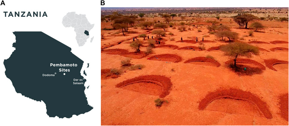
Figure 1. (A, B) A locator map (A) showing the location of the two bunds sites of Justdiggit in Pembamoto, Dodoma Region, Tanzania and a photo of several bunds in one of the two sites. Sources: Natural Earth and Projection Wizard (Šavrič et al., 2016) (A) and Justdiggit (B).

In the present work, we investigated the potential of several low resolution (e.g., 1–25 km), medium resolution (e.g., 100–250 m) and high resolution satellite data products (e.g., 3–4 m) (Supplementary Table S1) for detecting restoration effects. As displayed in Figure 2, a stepwise approach was followed to study this potential for two restoration intervention areas (Supplementary Figure S1). First, the optical scanning of the land surface provided a quick feasibility check to determine whether the expected increase in vegetation growth is indeed visible at high resolution. Otherwise, water and temperature effects due to increased vegetation are not likely to be detectable at low and medium resolution. Second, to study the baseline conditions and potential changes in soil and vegetation properties, temporal analysis of differences between intervention and control areas (see the Methods section and Supplementary Figure S1 on control area selection) was applied on the long-term (e.g., 10–44 years) datasets at lower resolution. Third, this temporal analysis was extended to medium resolution datasets to better understand and quantify the vegetation-water-temperature dynamics and effects of landscape restoration. Lastly, based on a co-design approach with Justdiggit, a translation of the quantified changes into user-friendly metrics was explored.

Figure 2

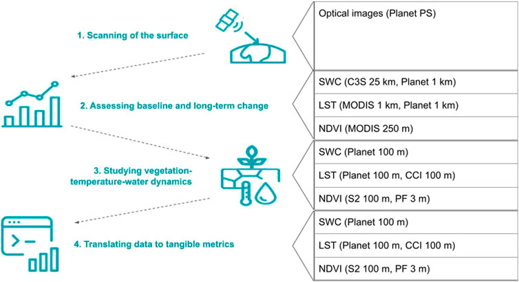
Figure 2. Workflow of the stepwise approach and the datasets considered per step. All dataset abbreviations are explained in Section 2.1.

2 Materials and methods

2.1 Data sources

In the current work, we have used the following products over the case study areas: PlanetScope (PS) daily scenes at 3.7 m resolution, C3S Passive Soil Moisture (here referred to as C3S soil water content, C3S SWC) 0.25°, Planet SWC 1 km, Planet SWC and LST 100 m, ESA CCI MODIS LST 1 km, ESA CCI Sentinel-3 (S3) LST 100 m, MODIS NDVI 250 m and Sentinel-2 NDVI 10 m and Planet Fusion 3 m (Planet Labs PBC Team, 2023). The latter was resampled to 100 m for comparison purposes. Please see Supplementary Table S2 for more details on the datasets’ specifications. Outliers in the datasets that are higher than three times the standard deviation have been removed. For the moving averages we applied a 20-days backwards looking window.

The long-term datasets (C3S SWC, CCI MODIS LST 1 km and MODIS NDVI) have an observation period that is long enough to establish a reasonable baseline. However, these datasets have either a low resolution (approximately 1–25 km resolution) or a low temporal resolution (once every 16 days). On the contrary, PS’s daily scenes offer the possibility to see daily visible changes with high spatial detail which allows for monitoring relative vegetation changes of small-scale interventions and determining the restoration area extent. The medium-resolution datasets (the downscaled 100 m SWC and LST) can capture more subtle changes in soil water and surface temperature properties that can be quantified in absolute values (de Jeu et al., 2017).

2.2 Study area and control area selection

This study focuses on two intervention areas near Pembamoto in the Dodoma region in Tanzania, the West Bunds area (centered at 6.2599°S 36.8142°E) and East Bunds area (centered at 6.2527°S 36.8431°E), as displayed by Figure 1 and Supplementary Figure S1. The bund areas are approximately 60 and 19 ha for the West and East Bunds areas, respectively. For both areas bunds have been dug from October to November 2018, after which grass seeds have been planted and the grazing restricted for the period studied.

The temporal variability of vegetation is mainly driven by the seasonal development cycle (one or more) and the inter-annual climate variability (Meroni et al., 2017). For soil water content and temperature there is also a very strong daily variation based on short-term weather conditions. The more types of fluctuations, the harder to differentiate between the effects of the intervention and other variations. Assuming that climatic conditions are rather homogeneous in the direct surroundings of the intervention area, comparing the conditions of the intervention area before and after the intervention with those of similar areas nearby helps to attribute ecosystem changes related to the intervention (Zucca et al., 2015; Meroni et al., 2017; Gann et al., 2019; Lindenmayer, 2020). Hence the selection of such control sites is required. For each control area, there could be project-control differences that are not related to the restoration interventions, for example, because of differences in natural variability or the presence of other anthropogenic interferences in the control areas. To reduce this uncertainty related to the selection of a single control site, we considered four different control sites per bunds area and averaged over the project-control differences. Supplementary Figure S1 displays the shapes and locations of the bunds and the control sites near Pembamoto in Tanzania. Control 1 is a randomly selected control site that is nearby the project area and approximately similar in size; Control 2 is a buffer of 1 km around the boundary of the project area; Control 3 is a buffer of 2 km where the part that overlaps with the 1 km buffer of Control 2 is excluded; and Control 4 is an expert selected control site selected by Justdiggit representing an “ideal” control site. Here an “ideal” control site is a nearby area that has similar conditions and is not perturbed by anthropogenic interferences. In contrast with control area 4, the other control areas were chosen to represent a more automated control area selection that is independent of local information. For the C3S SWC dataset, the West Bunds control areas fall in the same pixel as the respective project area. For this dataset the control areas should ideally be selected farther away from the project area, but for equal comparison we kept the control area selection the same for all datasets.

2.3 Impact definition and quantification

Green’s (1979) Before-After Control Impact (BACI) design was applied, comparing the observations between an intervention area and a control area, for the period before and after the intervention. Here multiple control areas were considered. This design helps to distinguish the impact of the intervention from pre-existing differences between intervention and control areas, especially when several control sites were considered (Underwood, 1994; del Río-Mena et al., 2023). We defined a “before” period: 2017-10-01 to 2018-09-30 and an “after” period: 2020-10-01 to 2021-09-30. The “before” period was chosen based on overlap in data availability of the medium-resolution datasets before the intervention took place and was limited to 1 year to avoid oversampling in a specific season. The “after” period was chosen to have the same duration and time of the year as the “before” period. Please note that for TIR LST no data was available in 2021, so we used the periods from 2016 to 10-01 to 2017-09-30 (i.e., before average) and from 2019 to 10-01 to 2020-09-30 (i.e., after average). To estimate the absolute change (i.e., possible impact) for each ecosystem variable, we computed the “before” and “after” average difference between the project area spatial mean and the average of all control area spatial means, and subtracted the latter from the former. For the long-term datasets, we computed the “before” average for the total period available before the bunds digging period and the “after” average for the total period available after the bunds digging period. To normalize the data we used

$x_{norm}=\frac{x-x_{\mathit{min}}}{x_{\mathit{max}}-x_{\mathit{min}}}.$

So the normalized change equals:

$norm.change={\overline{norm\left(x_p-x_c\right)}}_{after}-{\overline{norm\left(x_p-x_c\right)}}_{before},$

where the bar sign represents the average of that part of the equation. We computed the relative change as follow:

$rel.change\left(\%\right)=\frac{{\overline{\left(x_p-x_c\right)}}_{after}-{\overline{\left(x_p-x_c\right)}}_{before}}{{\overline{\left(x_p\right)}}_{before}}\times 100,$

where $x_p$ are the project area daily values and $x_c$ the average control areas daily values. Please note that the LST changes are computed relative to the before intervention project average in degrees Celsius.

2.4 Statistical trend analysis

Statistical trend analysis is applied on the complete time series of absolute daily project-control differences of each variable to study the sign and significance of trends. See Supplementary Figure S1 for the available observation period per dataset. Because of the variation in type of distribution of the project-control differences of the studied variables, a commonly used non-parametric test was chosen, the Mann-Kendal test. As these variables have a strong seasonal component, they are characterized by serial autocorrelation. Without correcting the time series for autocorrelation, trend test results can be misinterpreted. Whereas the seasonal Kendall test (Hirsch et al., 1982; Hirsch and Slack, 1984; Zetterqvist, 1991) eliminates the effect of seasonal dependence, it does not correct for time dependencies of the observations within seasons. However, intra-seasonal dependencies such as the diurnal temperature cycle and stationary weather fronts are also present in the timeseries. Therefore, the Hamed Rao Modified Mann Kendall trend test (one-tail, ɑ = 0.05) was applied, which uses variance correction to correct for serial autocorrelation (Hamed and Rao, 1998). The Hamed Rao Modified Mann Kendall test takes into account all significant lags with respect to autocorrelation.

3 Results

3.1 Scanning the surface for visible changes of ecosystem restoration

By studying Planet’s PlanetScope (Planet PS) images in May 2018, 2020 and 2022, regreening is clearly noticeable for the two case study areas. Figure 3 shows the growth of vegetation for one of the bunds areas near Pembamoto.

Figure 3

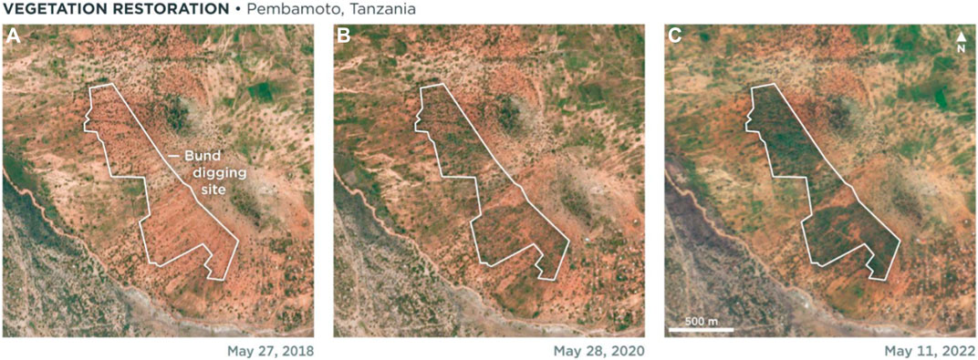
Figure 3. Planet PS images of May 2018 (A), 2020 (B) and 2022 (C) of the Justdiggit West Bunds area in Tanzania. The bunds digging site can be seen outlined in white.

3.2 Long-term satellite observations for baseline and change assessment

In the low resolution soil water content datasets, the EU’s Copernicus Climate Services Soil Water Content (C3S SWC) and Planet Soil Water Content 1 km (Planet SWC 1 km) datasets, there are no clear changes visible or found statistically significant (p > 0.10) for the project-control differences between the before and after bunds digging periods (see Supplementary Table S1). Please note that the West Bunds and East Bunds areas equal 0.001 and 0.0003 pixel of the C3S SWC dataset respectively. For the West Bunds area there are no differences observed at all, because the control areas fall in the same pixel as the project area. A distinct change in the Moderate Resolution Imaging Spectroradiometer Normalized Difference Vegetation Index (MODIS NDVI) at 250 m resolution is clear from Figure 4 and when looking more carefully also in the European Space Agency’s (ESA) Climate Change Initiative (CCI) MODIS LST at 1 km resolution. For MODIS NDVI the observed change is significant at the 95% confidence level for both bunds areas (Supplementary Table S1). The average increase in project-control differences of MODIS NDVI is 23%–30% with respect to the climatological average before bunds digging for the two bunds areas. For CCI MODIS LST the change is still statistically significant for the West Bunds area (p < 0.01), but not for the East Bunds area (p = 0.087). For the West Bunds area, the average increase in project-control differences of CCI MODIS LST is −13% with respect to the climatological average before bunds digging.

Figure 4

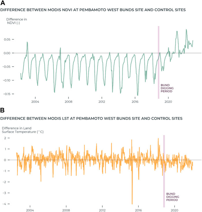
Figure 4. The differences in 20-day backward moving average MODIS NDVI (A) and CCI MODIS LST (B) between the West Bunds and the control area mean. The period of bunds digging (Oct-November 2018) is marked by the purple bar.

3.3 Vegetation-water-temperature dynamics at medium resolution

We found that the bunds areas stay mainly wetter and cooler than the average of the control sites after the bunds digging (Figures 3, 4 for the West Bunds area). When comparing the project-control average differences of the before-digging period and the after-bunds digging period, the East and West Bunds areas are 15% and 11% wetter than the control average respectively relative to the before intervention Planet SWC 100 m (here abbreviated as SWC) average corresponding to 0.009 and 0.007 m³ m⁻³ absolute average change. We found an average cooldown of 0.5°C and 0.4 °C for the East and the West Bunds area, which equals 1.5% and 1.1% cooldown with respect to control area average and relative to the average Planet microwave (MW) based LST of each bunds before the bunds digging. For the thermal-infrared (TIR) based LST, the absolute change detected is −0.15 °C and −0.33 °C with relative average change of −0.5% and −0.9% for the East and West Bunds areas respectively. For Sentinel-2 (S2) NDVI, we found that the East Bunds and West Bunds areas are on average 34%–37% greener than the reference for the period after bunds digging compared to the period before bunds digging. The highest relative average change, 55%–72% increase, was observed for Planet Fusion (PF) NDVI. The average spread between control area comparisons in SWC and MW LST has a similar order of magnitude as the average differences, 0.010–0.013 m³ m⁻³ (14%–16% relative the average SWC) and 0.65°C–0.82°C for the East and West Bunds respectively. However, the spread in project-control area comparisons continues to increase above (below) the zero-difference line in time for SWC (LST) for the West Bunds area, as seen in Figures 5, 6, and this has also been observed for the East Bunds area. Both the magnitude of the differences and the spread in control area comparisons vary seasonally, likely related to precipitation and vegetation patterns. Only for PF the mean spread in project-control area comparisons is about half of the absolute change, whereas for TIR LST this spread is six to 10 times larger than the absolute change. The largest positive differences in SWC associated with negative differences in MW LST are found for higher NDVI values (Figure 7).

Figure 5

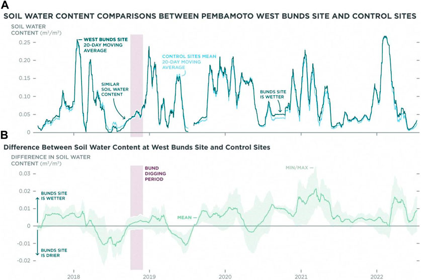
Figure 5. The top graph (A) visualizes the 20-day backward moving averages of SWC of the Pembamoto West Bunds site (dark blue) and the mean of the nearby control sites (light blue line) in time. The bottom graph (B) shows the differences in SWC with respect to the control area mean (solid green line) over the years. The minimum-maximum range of all project-control area comparisons is marked by the half-transparent light green color.

Figure 6

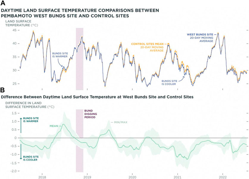
Figure 6. The top graph (A) visualizes the 20-day backward moving averages of daytime MW LST of the Pembamoto West Bunds site (blue) and the mean of the control sites (orange) over the years. The bottom graph (B) shows the differences in MW LST with respect to the control area mean (solid light blue line) in time. The minimum-maximum range of all project-control area comparisons is marked by the half-transparent light blue color.

Figure 7

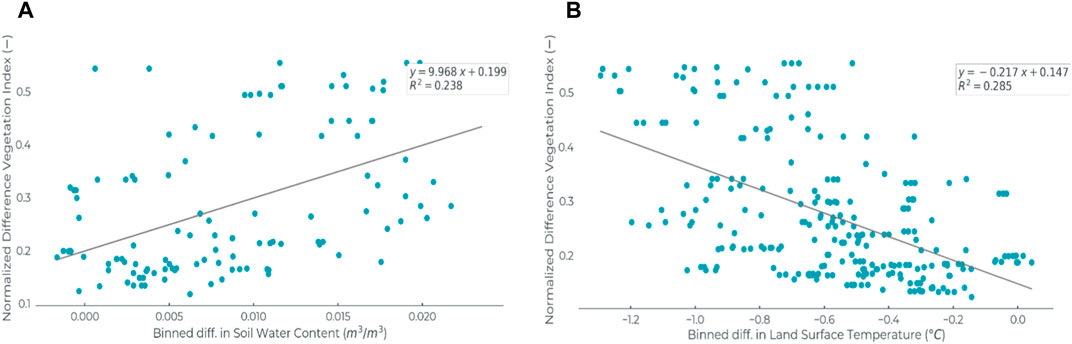
Figure 7. Differences in 10-day centered moving average SWC (A) and MW LST (B) compared to S2 NDVI values for the East Bunds area after bund digging.

The seasonal dynamics, inter-control spread and trends of the project-control differences in the different variables are coherent in time across the datasets of different temporal and spatial resolutions (Figure 8). Whereas indications of change could not be detected in the low resolution datasets of SWC (C3S SWC, Planet SWC 1 km) and LST (MODIS and Planet 1 km), the medium resolution datasets of SWC and LST do capture noticeable change that is comparable in dynamics to the observed MODIS and Sentinel NDVI change. Although the MODIS NDVI picks up the restoration effects on vegetation greenness, suggesting that the 250 m resolution is sufficient here, we do see it is less sensitive than PF NDVI.

Figure 8

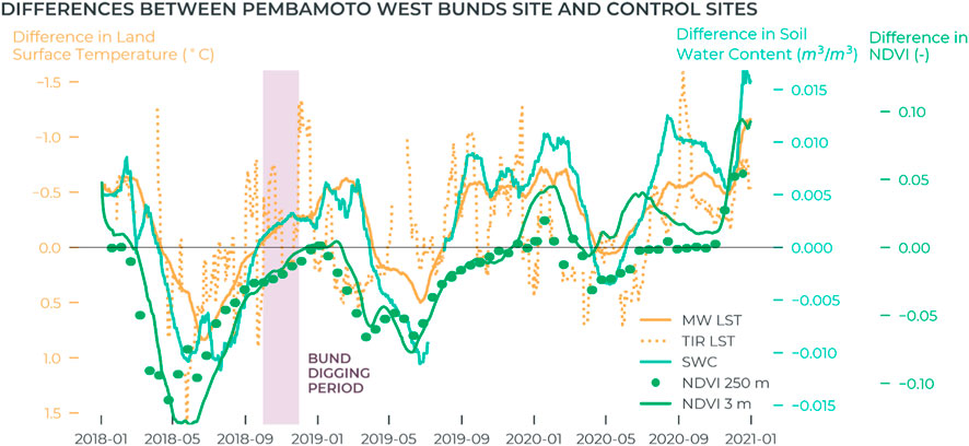
Figure 8. The differences in MW LST 100 m (solid orange line, inversed), TIR LST 100 m (dotted orange line), SWC 100 m (solid blue line), MODIS NDVI 250 m (green dots) and PF NDVI 3 m (solid green line) between the West Bunds area and the control area mean in time. The period of bunds digging (Oct-November 2018) is marked by the purple bar.

Modified Mann Kendall trend analysis was applied on the project-control mean differences of each variable for the period after bunds digging. Significant trends were found at the p = 0.001–0.05 significance levels (Table 1, except for TIR LST for the East Bunds area) with slopes of approximately $5e^{-6}{m}^3{m}^{-3}$ in SWC, $0.5e^{-4}$–$0.9e^{-4}$ in NDVI and ${2e}^{-4}$–${3e}^{-4}℃$ in MW LST per day. The sign of the slope was observed positive for SWC and NDVI and negative for MW and TIR LST. The NDVI trends are the most significant of all, even for MODIS NDVI where only approximately 170 observations were available. When excluding the before intervention period in this trend analysis the p values increase generally (Supplementary Table S3). Trends are then observed at 0.01%–10% significance levels with slopes that are approximately twice as small for the East Bunds while staying approximately the same for the West Bunds. The only deviating finding here is for TIR LST for the East Bunds where the p-value decreases to 0.11 and the slope becomes three times as big. In terms of relative average changes of the project-control differences between the before and after intervention period, we find 11% and 15% increases in SWC, 37% and 34% increases in S2 NDVI, 72% and 55% increases in PF NDVI, −1.1% and −1.5% decreases in MW LST and −0.9% and −0.5% decreases in TIR LST for the West and the East Bunds areas respectively. To compare the magnitude of the changes between the variables, the normalized changes were considered. The order of magnitude for the MW SWC, MW LST and S2 NDVI normalized changes is equal (e.g., ∼0.20). For PF NDVI the order of magnitude is similar, but twice as big (e.g., ∼0.4), whereas for the TIR LST we find normalized changes that are one order lower in magnitude (e.g., ∼0.02).

Table 1

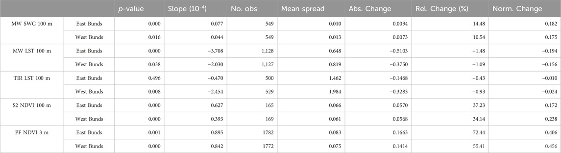
Table 1. Table including the Hamed Rao Modified Mann-Kendall trend results for the medium and high resolution datasets over the total available period and the changes in before—after averages, both for the project—control mean differences of multiple data products and the two bunds areas. The slope is the trend slope (average change per day).

3.4 From data to insights

The bunds-control area mean differences in microwave-based daytime temperature demonstrate that the bunds have the potential to cool down the topsoil 0.4°C–0.5°C on average over the observed period (October 2018 to July 2022, ∼3.5 years). Considering the difference plots of the West and East Bunds we found an average increase of 0.007–0.009 m³ m⁻³ in 3.5 years. For both bunds areas combined, the total extra retention of water for the top 10 cm of the soil as measured by the SWC data was estimated to equal approximately 615,000 L in 3.5 years. As this satellite-based analysis captures data from the top 10 cm of the soil only, the total extra retention number is a conservative estimate as the retention is expected to increase over a deeper soil layer (i.e., over the total grass root depth). For NDVI, only relative numbers can be computed, indicating that on average the bunds areas became approximately 35% (based on S2 NDVI) to 62% (based on PF NDVI) greener in 3.5 years. The area that is (partially) regreened can also be a metric, which is here approximately 80 ha in total.

4 Discussion

The increase in greenness visible in PS images of the bunds areas is in line with the observed trends in SWC, MW LST and S2 NDVI project-control differences, together demonstrating the effectiveness of the landscape regreening interventions. An increased infiltration through the digging of bunds has likely led to increased retention of soil water content which may have resulted in accelerated vegetation growth. This vegetation growth is expressed by NDVI and shown by the visual change of barren soil to green vegetation in PS imagery. This in turn could have led to cooling down the surface at daytime, which is represented by MW- and TIR-based daytime LST and in line with Feldman et al., 2022 through increased transpiration and a further increase of the soil water retention by plant roots (Wu et al., 2016; Feldman et al., 2023; He et al., 2023). The latter is reflected by MW SWC and in line with Wu et al., 2016; He et al., 2023. For the TIR LST, the trend in project-control differences is less clear, but still significant for the biggest project area (e.g., the West Bunds area). Potentially, the level of spatial detail is larger in the MW LST, than the TIR LST because of differences in downscaling methods. Other differences between TIR-based and MW-based LST are related to differences in the type of signal, sensitivity to clouds, retrieval algorithms, their dependence on auxiliary datasets, and penetration depth (Li et al., 2013; Zhang et al., 2019). In general, TIR retrievals are more accurate than MW retrievals (Nie et al., 2020). This is principally due to a stronger dependence of the radiance on temperature and smaller variation of surface emissivities (Zhang et al., 2019).

Whereas the long-term low resolution datasets are required to establish a baseline, medium to high resolution satellite-derived datasets capture enhanced spatial detail to help differentiate subtle spatial variation in vegetation-water-temperature dynamics and effects of landscape restoration. The available 1 km datasets of SWC and MW LST are not sensitive enough to determine the changes for this type and spatial scale of landscape restoration and a resolution of 100 m was a necessity to capture these changes. The medium resolution SWC, MW LST and S2 NDVI datasets made it possible to study the interaction between water, temperature and vegetation growth within restored landscapes, which gave a better understanding of the mechanisms and uncertainties. Hence, this study demonstrated the necessity for medium to high resolution satellite observations. The biggest differences in SWC and MW LST are found for higher S2 NDVI values, which matches the proposed relationship between an increase in plant growth (expressed by an increase in plant greenness) and an increase in the water holding capacity of the soil (represented by SWC) and higher transpiration leading to lower LST values.

When comparing the normalized changes, we see that those of PF NDVI at 3 m resolution are two times as big as those of the other datasets at 100–250 m resolution. This might indicate that higher spatial resolution more fully captures the restoration effects. In addition, when comparing the NDVI changes at 250 m and the SWC and LST changes at 100 m resolution, the order of magnitude of change is similar. This could imply that the vegetation effects are more easy to detect than the SWC and LST effects (similar order of magnitude for 100 m vs. 250 m resolution datasets), which might be explained by the differences in physical dynamics of the variables. For example, the main changes in vegetation greenness are driven by the availability of water, which is improved due to the intervention and varies seasonally based on precipitation patterns and the amount of evapo-transpiration (Jia and Shao, 2014). For the SWC and LST also other processes play a role in the short- and long-term variations, likely explaining why these variations are a bit harder to detect. For example, some of the increased SWC is immediately used by the grasses to grow (Jia and Shao, 2014). Similarly for temperature, there is a balance between a warming effect through decreased albedo and a cooling effect through increased transpiration and wetter soils with more (wet) vegetation that will be sensed cooler (Chapin et al., 2008; Zhang et al., 2013). Here we observe a net cooling effect of the regreening intervention, which is in line with the findings of Feldman et al., 2022 for temperate vegetation (Feldman et al., 2023). As it has not been determined how long the intervention is still affecting the observed dynamics, please note that the change numbers computed in this study do not reflect the total before-after change.

The lowest resolution dataset for which a significant change was detected for the West Bunds area, is the 1 km resolution (e.g., CCI MODIS LST) corresponding to a spatial coverage of 0.6 pixels of the project area. Although no significant changes were found for the East Bunds area with the 1 km resolution datasets, which cover 0.3 pixels of the project area, significant changes were detected for resolutions of 250 m or higher, corresponding to a coverage of 3 or more pixels of the project area. This might suggest that the restoration area size needs to equal at least half a pixel of spatial data coverage for the dataset to be able to detect any restoration effects. This corresponds to Cowen et al. (1995), which states that it also depends on the pixel alignment with respect to the object to be identified and the actual level of spatial detail in the dataset (Cowen et al., 1995; Myint et al., 2011). In a study of Thorton et al. (2007) pixel size needed to be bigger than half a pixel to detect rural land cover objects while using sub-pixel mapping that adjusts for pixel misalignment (Thornton et al., 2006). Note that the restoration also included grazing restrictions which could have led to impact across the border of the intervention areas, which might have helped in detecting these trends for areas that cover half a pixel. Differences in the magnitude and significance of trends between the West and East Bund areas can be explained by the different area sizes and potential differences in “before” conditions, type of vegetation, land use in control areas and the density and size of bunds.

We observed seasonality in the project-control differences before the bunds digging, which is likely related to the presence of some vegetation in the control areas before the bunds digging. From this we can conclude that we do not have a perfect reference that equals the surface conditions of the project area before the bunds digging. A perfect reference should also not differ from the project area in terms of natural variability or perturbation by anthropogenic interferences for the period after the bunds digging (Meroni et al., 2017). Beyond the scope of the current study, a more automated control area selection as described in Meroni et al. (2017) could be adapted in future studies when extended in the following three manners (Meroni et al., 2017). Firstly, studying the climatologies of the relevant variables, for example, SWC, LST, NDVI, to find control areas that have similar natural variability as the project area before bund digging. Secondly, a non-visual check whether significant changes occur in the control areas for the entire before-after period. Thirdly, these studies should include the requirement that each control area is selected from a different pixel concerning the dataset of lowest resolution.

Admittedly, a reason for debating the attribution of the observed differences to the restoration interventions is that the absolute differences are within the order of the average dataset accuracy (up to 0.04 m³ m⁻³ RMSE for SWC) or even one order lower (2°C–3°C RMSE daytime for MW LST and 1°C–2°C RMSE for TIR LST) (Calvet et al., 2011; Gao et al., 2018; Tan et al., 2019; Zheng et al., 2019; Yang et al., 2020; Ye et al., 2021). However, as we are considering the differences between two soil water content values, one might assume that the error in the difference is canceled out for a long enough sample size. Moreover, we find significant trends in the differences and it is unlikely that the measurement error is time dependent. The likelihood of false attribution of project-control differences related to the specific choice of the control area is reduced by taking the average of four control areas per project area as the reference. Similarly, false attribution of these differences because of local changes in weather conditions between the project and control areas for the period of interest of the medium resolution datasets (e.g., 2017–2020) can be considered negligible. As the differences are based on the average of all project-control differences, one might assume that these changes or trends in small-scale weather differences are canceled out (Conner et al., 2016). Besides, the trends observed in the different independent variables are consistent and in line with the expected effects of landscape regreening. However, extending the medium resolution datasets (now starting in 2017) with longer time records (e.g., Landsat, AMSR2 and/or AMSRE) would help to shed more light on the robustness of the current findings of the medium resolution datasets, as it would allow for a better distinction between the natural variability and restoration impact. However, as the MODIS NDVI project-control timeseries does provide a good baseline and is coherent in temporal dynamics, inter-control spread and trends with the SWC and MW LST differences, it is likely that the observed SWC and MW LST changes can be attributed as restoration effects. Whereas a short before period that would be particularly dry (warm) could have led to false wettening (cooling) trends, the MODIS NDVI timeseries shows that this was not the case.

However, Serinaldi et al. (2018) recommended to use trend tests not to infer nonstationarity, but only as preliminary screening to identify possible upward or downward processes. For these changes a clear physical mechanism concerning the predictable evolution of the properties of the related process is required, to draw any conclusions about the trend results (Serinaldi et al., 2018). In this case the significant changes are physically meaningful as they are related to a well defined physical intervention at a known point in time justifying causality, here the construction of the bunds. More research is needed to increase the confidence of the satellite products’ ability to measure restoration effectiveness in time. This research should include more research areas in different hydro-climatic regions at different scales (ranging from 0.1 to 100 km² when available) and restoration activities of various restoration types and starting dates (e.g., 2–20 years old).

The current approach uses high-resolution optical imagery to investigate the likelihood of detecting trends in vegetation, water and temperature datasets at medium resolution in time. Although many restoration activities are likely to result in visible land surface changes (e.g., bunds, irrigation channels, grass banks), this does not have to be the case for micro-scale interventions such as agroforestry applied on a bigger region. In these conditions, it could still be worthwhile to analyze the temporal changes and trends. Whereas, the current work focuses mainly on the temporal component of ecosystem change, it would be interesting to also analyze associated spatial patterns and their changes in times as in T. del Rio-Mena et al. (2023) (Río-Mena et al., 2021). This will give more insights in the underlying processes and provides spatial validation of the effects of landscape restoration.

Further investigation of the relationship between SWC and vegetation growth would allow better understanding of the magnitude of the effects of landscape restoration. This would also help to better distinguish between seasonal variability and restoration effects. Deep soil water layers can also be depleted due to revegetation when the actual evaporation is higher than the precipitation and runoff is not necessarily decreased because of the revegetation (Jia and Shao, 2014; Qiu et al., 2021). Therefore, the analysis of deep SWC as well as the amount of water retention by vegetation, would allow for a better estimation of the total retention of water in the soil and in vegetation in the bunds areas. Please note that even when water retention at the local scale is not benefited from restoration, increased evapotranspiration will induce the cross-continental transport of moisture vapor, and hence increase precipitation in areas distant from the ocean-based hydrological cycle (Ellison et al., 2012; von Holle et al., 2020).

Regarding the translation of the results into insights, multi-disciplinary expertise and further co-designing of usefulness metrics with stakeholders is required to extend the first attempts presented here. Thereby investigating which metrics express impact of restoration in both a scientifically correct and user-friendly way and work across spatial scales and restoration types. For users like Justdiggit that need to communicate transparently and regularly to their stakeholders (Buckingham et al., 2019), operationalization is key, as they currently face challenges in conducting this in a scalable and cost-effective manner. An operational monitoring service would require continuity, scalability, reliability (e.g., accuracy and backup possibilities for satellite outages), efficient processing to the spatial and temporal resolution necessary and sufficient latency (IPBES, 2018). Hence, operationalization of the proposed workflow and the underlying data and insight delivery supports effective decision and policy making. This paves the way to more effective restoration encouraging investors, governments and communities to restore more land (Buckingham et al., 2019).

5 Conclusion

Satellite data observations of different spatial and temporal scales indicate that the digging of bunds and related grazing restriction has promoted vegetation growth (∼50% greener on average, p ≤ 0.001), top-layer soil water retention (∼13% average increase, p < 0.02) and soil cooling (∼-0.5°C, p < 0.04) over the study regions in Tanzania. Moving to resolutions higher or equal to 250 m led to more significant and pronounced trends and made it possible to study the interaction between water, temperature and vegetation growth. The presented approach is a cost-effective and objective method to monitor the effectiveness of landscape regreening efforts. Repeating this temporal study over more areas, at different soil depths and extending it with spatial analysis is needed to further increase our understanding of the magnitude of regreening effects and the confidence of the satellite products’ ability to measure restoration effectiveness in time. When the results are translated to more user-friendly metrics, operationalized, and complemented with local insights and data, this method can help to make restoration more effective and quantifiable. All in all, we conclude that high quality satellite observations from space agencies and commercial providers are now achieving the frequency, resolution, and accuracy needed to evaluate and monitor restoration activities.

6 Restore-IT consortium

Planet Labs PBC, Earth Observation Lab, Haarlem, Netherlands, Mendy van der Vliet, Richard A. M. de Jeu, Yoann Malbeteau. National Centre for Earth Observation; Department of Physics and Astronomy, University of Leicester, Leicester, United Kingdom Darren Ghent, Karen L. Veal, Justdiggit, Amsterdam, Netherlands. Sander de Haas, Thijs van der Zaan, Department of Earth Sciences, Indian Institute of Technology Kanpur, Kanpur, India. Rajiv Sinha, Saroj K. Dash, Planet Labs PBC, San Francisco, CA, United States, Rasmus Houborg.

Data availability statement

The datasets presented in this article are not readily available because The C3S SWC dataset is publicly available at https://cds.climate.copernicus.eu/cdsapp#!/dataset/satellite-soil-moisture (DOI: 10.24381/cds.d7782f18). The CCI MODIS LST 1 km dataset is freely available at https://climate.esa.int/en/odp/#/project/land-surface-temperature and archived at https://data.ceda.ac.uk/neodc/esacci/land_surface_temperature/data/MULTISENSOR_IRCDR/L3S/0.01/v2.00/monthly. The MODIS and S2 NDVI data can be retrieved from the Google Earth Engine (https://earthengine.google.com/). PlanetScope images are available under a license from the Education and Research programme from Planet Labs PBC (Planet Labs PBC Team, 2023; RRID:SCR_024689). The other data that support the findings of this study (e.g., csv files of region-of-interest averages of Planet SWC, LST and PF for the project and control areas over the observation period) will be made available upon request. Requests to access the datasets should be directed to Mendy van der Vliet, mendyvandervliet@planet.com.

Author contributions

MV: Conceptualization, Data Curation, Formal Analysis, Funding Acquisition, Investigation, Methodology, Project Administration, Software, Visualization, Writing–Original Draft. YM: Data Curation, Formal Analysis, Software, Writing–Review and Editing. DG: Data Curation, Writing–Review and Editing. SH: Resources, Writing–Review and Editing. KV: Data Curation, Writing–Review and Editing. TZ: Resources, Writing–Review and Editing. RS: Writing–Review and Editing. SD: Writing–Review and Editing. RH: Data Curation, Writing–Review and Editing. RJ: Conceptualization, Methodology, Supervision, Writing–Review and Editing.

Funding

The author(s) declare that financial support was received for the research, authorship, and/or publication of this article. Funding for this study was provided by ESA in the framework of the EO4Society open call project Restore-IT (project no. ESA-CIP-POE-DT-lr-sp-LE-2021-716, contract no. 4000136484/21/I-DT-lr).

Acknowledgments

We acknowledge the help of M. Klink and T. Davis with part of the data preparation for this analysis. We thank Marc Pagani for his valuable advice and S. van Schijndel for her organizational contribution to the project. We thank L. Texeira, S. Levay, L. Neville, J. Schellekens and T. Davis who generously provided their extensive feedback on this manuscript and M. Borrmann, J. Peschel and R. Simmon for contributing to the visualization of Figures 1, 2, 5, 6. We acknowledge the use of imagery from the Copernicus Climate Data Store (e.g., C3S SWC) and Google Earth Engine (e.g., MODIS and Sentinel-2 NDVI). The findings and views described herein do not necessarily reflect those of Planet Labs PBC. The manuscript is based on the following preprint: https://www.researchsquare.com/article/rs-2669521/v1 (van der Vliet et al., 2023).

Conflict of interest

The authors declare the following financial interests/personal relationships which may be considered as potential competing interests: MV, RJ, YM, and RH were employed by Planet Labs PBC.

The author(s) declared that they were an editorial board member of Frontiers, at the time of submission. This had no impact on the peer review process and the final decision.

Publisher’s note

All claims expressed in this article are solely those of the authors and do not necessarily represent those of their affiliated organizations, or those of the publisher, the editors and the reviewers. Any product that may be evaluated in this article, or claim that may be made by its manufacturer, is not guaranteed or endorsed by the publisher.

Supplementary material

The Supplementary Material for this article can be found online at: https://www.frontiersin.org/articles/10.3389/fenvs.2024.1352058/full#supplementary-material

References

Abiye, W. (2022). Soil and water conservation nexus agricultural productivity in Ethiopia. Adv. Agric. 2022 2022, 1–10. doi:10.1155/2022/8611733

CrossRef Full Text | Google Scholar

Andres, L., Boateng, K., Borja-Vega, C., and Thomas, E. (2018). A review of in-situ and remote sensing technologies to monitor water and sanitation interventions. Water 10, 756. doi:10.3390/w10060756

CrossRef Full Text | Google Scholar

Atkinson, J., Brudvig, L. A., Mallen-Cooper, M., Nakagawa, S., Moles, A. T., and Bonser, S. P. (2022). Terrestrial ecosystem restoration increases biodiversity and reduces its variability, but not to reference levels: a global meta-analysis. Ecol. Lett. 25, 1725–1737. doi:10.1111/ele.14025

PubMed Abstract | CrossRef Full Text | Google Scholar

Belayneh, M., Yirgu, T., and Tsegaye, D. (2020). Runoff and soil loss responses of cultivated land managed with graded soil bunds of different ages in the Upper Blue Nile basin, Ethiopia. Ecol. Process. 9, 66–18. doi:10.1186/s13717-020-00270-5

CrossRef Full Text | Google Scholar

Buckingham, K., Ray, S., Granizo, C. G., Toh, L., Stolle, F., Zoveda, F., et al. (2019). The road to restoration.

Google Scholar

Calvet, J.-C., Wigneron, J.-P., Walker, J., Karbou, F., Chanzy, A., and Albergel, C. (2011). Sensitivity of passive microwave observations to soil moisture and vegetation water content: L-band to W-band. IEEE Trans. Geosci. Remote Sens. 49, 1190–1199. doi:10.1109/TGRS.2010.2050488

CrossRef Full Text | Google Scholar

Capdevila, P., Stott, I., Oliveras Menor, I., Stouffer, D. B., Raimundo, R. L., White, H., et al. (2021). Reconciling resilience across ecological systems, species and subdisciplines. Wiley Online Library.

Google Scholar

Chapin, F. S., Randerson, J. T., McGuire, A. D., Foley, J. A., and Field, C. B. (2008). Changing feedbacks in the climate–biosphere system. Front. Ecol. Environ. 6, 313–320. doi:10.1890/080005

CrossRef Full Text | Google Scholar

Chimner, R. A., Bourgeau-Chavez, L., Grelik, S., Hribljan, J. A., Clarke, A. M. P., Polk, M. H., et al. (2019). Mapping mountain peatlands and wet meadows using multi-date, multi-sensor remote sensing in the Cordillera Blanca, Peru. Wetlands 39, 1057–1067. doi:10.1007/s13157-019-01134-1

CrossRef Full Text | Google Scholar

Conner, M. M., Saunders, W. C., Bouwes, N., and Jordan, C. (2016). Evaluating impacts using a BACI design, ratios, and a Bayesian approach with a focus on restoration. Environ. Monit. Assess. 188, 555. doi:10.1007/s10661-016-5526-6

PubMed Abstract | CrossRef Full Text | Google Scholar

Cowen, D. J., Jensen, J. R., Bresnahan, P. J., Ehler, G. B., Graves, D., and Huang, X. (1995). The design and implementation of an integrated geographic information system for environmental applications. Photogramm. Eng. Remote Sens. 61, 1393–1404.

Google Scholar

de Almeida, D. R., Stark, S. C., Valbuena, R., Broadbent, E. N., Silva, T. S., de Resende, A. F., et al. (2020). A new era in forest restoration monitoring. Restor. Ecol. 28, 8–11. doi:10.1111/rec.13067

CrossRef Full Text | Google Scholar

de Jeu, R. A. M., de Nijs, A. H. A., and Klink, M. H. W. V. (2017). Method and system for improving the resolution of sensor data. EU patent No WO2017216186A1. World intellectual property organization.

Google Scholar

del Río-Mena, T., Willemen, L., Tesfamariam, G. T., Beukes, O., and Nelson, A. (2020). Remote sensing for mapping ecosystem services to support evaluation of ecological restoration interventions in an arid landscape. Ecol. Indic. 113, 106182. doi:10.1016/j.ecolind.2020.106182

CrossRef Full Text | Google Scholar

del Río-Mena, T., Willemen, L., Vrieling, A., and Nelson, A. (2023). How remote sensing choices influence ecosystem services monitoring and evaluation results of ecological restoration interventions. Ecosyst. Serv. 64, 101565. doi:10.1016/j.ecoser.2023.101565

CrossRef Full Text | Google Scholar

Ellison, D., Futter, N., and Bishop, K. (2012). On the forest cover–water yield debate: from demand-to supply-side thinking. Glob. Change Biol. 18, 806–820. doi:10.1111/j.1365-2486.2011.02589.x

CrossRef Full Text | Google Scholar

Eva, H., Carboni, S., Achard, F., Stach, N., Durieux, L., Faure, J.-F., et al. (2010). Monitoring forest areas from continental to territorial levels using a sample of medium spatial resolution satellite imagery. ISPRS J. Photogramm. Remote Sens. 65, 191–197. doi:10.1016/j.isprsjprs.2009.10.008

CrossRef Full Text | Google Scholar

Feldman, A. F., Short Gianotti, D. J., Dong, J., Trigo, I. F., Salvucci, G. D., and Entekhabi, D. (2023). Tropical surface temperature response to vegetation cover changes and the role of drylands. Glob. Change Biol. 29, 110–125. doi:10.1111/gcb.16455

CrossRef Full Text | Google Scholar

Gann, G. D., McDonald, T., Walder, B., Aronson, J., Nelson, C. R., Jonson, J., et al. (2019). International principles and standards for the practice of ecological restoration. Second edition. Restor. Ecol. 27, S1–S46. doi:10.1111/rec.13035

CrossRef Full Text | Google Scholar

Gao, Y., Walker, J., Ye, N., Panciera, R., Monerris, A., Ryu, D., et al. (2018). Evaluation of the tau–omega model for passive microwave soil moisture retrieval using SMAPEx datasets. IEEE J. Sel. Top. Appl. Earth Obs. Remote Sens. PP, 888–895. doi:10.1109/JSTARS.2018.2796546

CrossRef Full Text | Google Scholar

Green, R. H. (1979). Sampling design and statistical methods for environmental biologists. John Wiley & Sons.

Google Scholar

Gross, J. E., Goetz, S. J., and Cihlar, J. (2009). Application of remote sensing to parks and protected area monitoring: introduction to the special issue. Remote Sens. Environ. 113, 1343–1345. doi:10.1016/j.rse.2008.12.013

CrossRef Full Text | Google Scholar

Gumma, M. K., Desta, G., Amede, T., Panjala, P., Smith, A. P., Kassawmar, T., et al. (2022). Assessing the impacts of watershed interventions using ground data and remote sensing: a case study in Ethiopia. Int. J. Environ. Sci. Technol. 19, 1653–1670. doi:10.1007/s13762-021-03192-7

CrossRef Full Text | Google Scholar

Güttler, F. N., Niculescu, S., and Gohin, F. (2013). Turbidity retrieval and monitoring of Danube Delta waters using multi-sensor optical remote sensing data: an integrated view from the delta plain lakes to the western–northwestern Black Sea coastal zone. Remote Sens. Environ. 132, 86–101. doi:10.1016/j.rse.2013.01.009

CrossRef Full Text | Google Scholar

Hamed, K. H., and Rao, A. R. (1998). A modified Mann-Kendall trend test for autocorrelated data. J. Hydrol. 204, 182–196. doi:10.1016/s0022-1694(97)00125-x

CrossRef Full Text | Google Scholar

Hansen, M. C., Stehman, S. V., Potapov, P. V., Loveland, T. R., Townshend, J. R., DeFries, R. S., et al. (2008). Humid tropical forest clearing from 2000 to 2005 quantified by using multitemporal and multiresolution remotely sensed data. Proc. Natl. Acad. Sci. 105, 9439–9444. doi:10.1073/pnas.0804042105

PubMed Abstract | CrossRef Full Text | Google Scholar

He, W., Ishikawa, T., and Nguyen, B. T. (2023). Effect evaluation of grass roots on mechanical properties of unsaturated coarse-grained soil. Transp. Geotech. 38, 100912. doi:10.1016/j.trgeo.2022.100912

CrossRef Full Text | Google Scholar

IPBES (2018). The IPBES assessment report on land degradation and restoration. Editors L. Montanarella R. Scholes A. Brainich. Bonn, Germany: Secretariat of the Intergovernmental Science-Policy Platform on Biodiversity and Ecosystem Services, 744. Available at: https://www.ipbes.net/assessment-reports/ldr

Google Scholar

IPCC (2022). “Contribution of Working Group II to the Sixth Assessment Report of the Intergovernmental Panel on Climate Change,” in Climate Change 2022: Impacts, Adaptation and Vulnerability. Editors H. O. Pörtner, D. C. Roberts, H. Adams, C. Adler, P. Aldunce, E. Aliet al. Cambridge, United Kingdom: Cambridge University Press, 3056. doi:10.1017/9781009325844

CrossRef Full Text | Google Scholar

Jia, Y.-H., and Shao, M.-A. (2014). Dynamics of deep soil moisture in response to vegetational restoration on the Loess Plateau of China. J. Hydrol. 519, 523–531. doi:10.1016/j.jhydrol.2014.07.043

CrossRef Full Text | Google Scholar

Lausch, A., Borg, E., Bumberger, J., Dietrich, P., Heurich, M., Huth, A., et al. (2018). Understanding forest health with remote sensing, part III: requirements for a scalable multi-source forest health monitoring network based on data science approaches. Remote Sens. 10, 1120. doi:10.3390/rs10071120

CrossRef Full Text | Google Scholar

Li, Z.-L., Tang, B.-H., Wu, H., Ren, H., Yan, G., Wan, Z., et al. (2013). Satellite-derived land surface temperature: current status and perspectives. Remote Sens. Environ. 131, 14–37. doi:10.1016/j.rse.2012.12.008

CrossRef Full Text | Google Scholar

Lindenmayer, D. (2020). Improving restoration programs through greater connection with ecological theory and better monitoring. Front. Ecol. Evol. 8, 50. doi:10.3389/fevo.2020.00050

CrossRef Full Text | Google Scholar

McDermid, G. J., Franklin, S. E., and LeDrew, E. F. (2005). Remote sensing for large-area habitat mapping. Prog. Phys. Geogr. 29, 449–474. doi:10.1191/0309133305pp455ra

CrossRef Full Text | Google Scholar

Meroni, M., Schucknecht, A., Fasbender, D., Rembold, F., Fava, F., Mauclaire, M., et al. (2017). Remote sensing monitoring of land restoration interventions in semi-arid environments with a before–after control-impact statistical design. Int. J. Appl. Earth Obs. Geoinformation 59, 42–52. doi:10.1016/j.jag.2017.02.016

PubMed Abstract | CrossRef Full Text | Google Scholar

Myint, S. W., Gober, P., Brazel, A., Grossman-Clarke, S., and Weng, Q. (2011). Per-pixel vs. object-based classification of urban land cover extraction using high spatial resolution imagery. Remote Sens. Environ. 115, 1145–1161. doi:10.1016/j.rse.2010.12.017

CrossRef Full Text | Google Scholar

Nagendra, H., Lucas, R., Honrado, J. P., Jongman, R. H., Tarantino, C., Adamo, M., et al. (2013). Remote sensing for conservation monitoring: assessing protected areas, habitat extent, habitat condition, species diversity, and threats. Ecol. Indic. 33, 45–59. doi:10.1016/j.ecolind.2012.09.014

CrossRef Full Text | Google Scholar

Nie, J., Ren, H., Zheng, Y., Ghent, D., and Tansey, K. (2020). Land surface temperature and emissivity retrieval from nighttime middle-infrared and thermal-infrared Sentinel-3 images. IEEE Geosci. Remote Sens. Lett. 18, 915–919. doi:10.1109/lgrs.2020.2986326

CrossRef Full Text | Google Scholar

Ockendon, N., Thomas, D. H., Cortina, J., Adams, W. M., Aykroyd, T., Barov, B., et al. (2018). One hundred priority questions for landscape restoration in Europe. Biol. Conserv. 221, 198–208. doi:10.1016/j.biocon.2018.03.002

CrossRef Full Text | Google Scholar

Pereira, H. M., Ferrier, S., Walters, M., Geller, G. N., Jongman, R. H., Scholes, R. J., et al. (2013). Essential biodiversity variables. Science 339, 277–278. doi:10.1126/science.1229931

PubMed Abstract | CrossRef Full Text | Google Scholar

Pettorelli, N., Laurance, W. F., O’Brien, T. G., Wegmann, M., Nagendra, H., and Turner, W. (2014). Satellite remote sensing for applied ecologists: opportunities and challenges. J. Appl. Ecol. 51, 839–848. doi:10.1111/1365-2664.12261

CrossRef Full Text | Google Scholar

Pettorelli, N., Schulte to Bühne, H., Tulloch, A., Dubois, G., Macinnis-Ng, C., Queirós, A. M., et al. (2018). Satellite remote sensing of ecosystem functions: opportunities, challenges and way forward. Remote Sens. Ecol. Conserv. 4, 71–93. doi:10.1002/rse2.59

CrossRef Full Text | Google Scholar

Planet Labs PBC Team (2023). Planet application program interface: in space for life on Earth. Available at: https://api.planet.com.

Google Scholar

Qiu, L., Wu, Y., Shi, Z., Yu, M., Zhao, F., and Guan, Y. (2021). Quantifying spatiotemporal variations in soil moisture driven by vegetation restoration on the Loess Plateau of China. J. Hydrol. 600, 126580. doi:10.1016/j.jhydrol.2021.126580

CrossRef Full Text | Google Scholar

Río-Mena, T. del, Willemen, L., Vrieling, A., Snoeys, A., and Nelson, A. (2021). Long-term assessment of ecosystem services at ecological restoration sites using Landsat time series. PLOS ONE 16, e0243020. doi:10.1371/journal.pone.0243020

PubMed Abstract | CrossRef Full Text | Google Scholar

Sacande, M., Martucci, A., and Vollrath, A. (2021). Monitoring large-scale restoration interventions from land preparation to biomass growth in the Sahel. Remote Sens. 13, 3767. doi:10.3390/rs13183767

CrossRef Full Text | Google Scholar

Šavrič, B., Jenny, B., and Jenny, H. (2016). Projection Wizard–An online map projection selection tool. Cartogr. J. 53, 177–185. doi:10.1080/00087041.2015.1131938

CrossRef Full Text | Google Scholar

Secades, C., O’Connor, B., Brown, C., and Walpole, M. (2014). Earth observation for biodiversity monitoring: a review of current approaches and future opportunities for tracking progress towards the Aichi Biodiversity Targets. CBD Tech. Ser. Available at: http://www.cbd.int/doc/publications/cbd-ts-72-en.pdf

Google Scholar

Serinaldi, F., Kilsby, C. G., and Lombardo, F. (2018). Untenable nonstationarity: an assessment of the fitness for purpose of trend tests in hydrology. Adv. Water Resour. 111, 132–155. doi:10.1016/j.advwatres.2017.10.015

CrossRef Full Text | Google Scholar

Stephenson, P. J., Burgess, N. D., Jungmann, L., Loh, J., O’Connor, S., Oldfield, T., et al. (2015). Overcoming the challenges to conservation monitoring: integrating data from in-situ reporting and global data sets to measure impact and performance. Biodiversity 16, 68–85. doi:10.1080/14888386.2015.1070373

CrossRef Full Text | Google Scholar

Tan, J., NourEldeen, N., Mao, K., Shi, J., Li, Z., Xu, T., et al. (2019). Deep learning convolutional neural network for the retrieval of land surface temperature from AMSR2 data in China. Sensors 19, 2987. doi:10.3390/s19132987

PubMed Abstract | CrossRef Full Text | Google Scholar

Thornton, M. W., Atkinson, P. M., and Holland, D. A. (2006). Sub-pixel mapping of rural land cover objects from fine spatial resolution satellite sensor imagery using super-resolution pixel-swapping. Int. J. Remote Sens. 27, 473–491. doi:10.1080/01431160500207088

CrossRef Full Text | Google Scholar

Underwood, A. J. (1994). On beyond BACI: sampling designs that might reliably detect environmental disturbances. Ecol. Appl. 4, 3–15. doi:10.2307/1942110

CrossRef Full Text | Google Scholar

van der Vliet, M., de Jeu, R., Malbeteau, Y., Ghent, D., Veal, K., de Haas, S., et al. (2023). Quantifiable impact: monitoring landscape restoration from space. doi:10.21203/rs.3.rs-2669521/v1

CrossRef Full Text | Google Scholar

von Holle, B., Yelenik, S., and Gornish, E. S. (2020). Restoration at the landscape scale as a means of mitigation and adaptation to climate change. Curr. Landsc. Ecol. Rep. 5, 85–97. doi:10.1007/s40823-020-00056-7

CrossRef Full Text | Google Scholar

Wu, G.-L., Yang, Z., Cui, Z., Liu, Y., Fang, N.-F., and Shi, Z.-H. (2016). Mixed artificial grasslands with more roots improved mine soil infiltration capacity. J. Hydrol. 535, 54–60. doi:10.1016/j.jhydrol.2016.01.059

CrossRef Full Text | Google Scholar

Yang, J., Zhou, J., Göttsche, F.-M., Long, Z., Ma, J., and Luo, R. (2020). Investigation and validation of algorithms for estimating land surface temperature from Sentinel-3 SLSTR data. Int. J. Appl. Earth Obs. Geoinformation 91, 102136. doi:10.1016/j.jag.2020.102136

CrossRef Full Text | Google Scholar

Ye, N., Walker, J. P., Wu, X., De Jeu, R., Gao, Y., Jackson, T. J., et al. (2021). The soil moisture active passive experiments: validation of the SMAP products in Australia. IEEE Trans. Geosci. Remote Sens. 59, 2922–2939. doi:10.1109/TGRS.2020.3007371

CrossRef Full Text | Google Scholar

Young, T. P., and Schwartz, M. W. (2019). The decade on ecosystem restoration is an impetus to get it right. Conserv. Sci. Pract. 1, e145. doi:10.1111/csp2.145

CrossRef Full Text | Google Scholar

Zhang, X., Tang, Q., Zheng, J., and Ge, Q. (2013). Warming/cooling effects of cropland greenness changes during 1982–2006 in the North China Plain. Environ. Res. Lett. 8, 024038. doi:10.1088/1748-9326/8/2/024038

CrossRef Full Text | Google Scholar

Zhang, X., Zhou, J., Göttsche, F.-M., Zhan, W., Liu, S., and Cao, R. (2019). A method based on temporal component decomposition for estimating 1-km all-weather land surface temperature by merging satellite thermal infrared and passive microwave observations. IEEE Trans. Geosci. Remote Sens. 57, 4670–4691. doi:10.1109/TGRS.2019.2892417

CrossRef Full Text | Google Scholar

Zheng, Y., Ren, H., Guo, J., Ghent, D., Tansey, K., Hu, X., et al. (2019). Land surface temperature retrieval from sentinel-3A sea and land surface temperature radiometer, using a split-window algorithm. Remote Sens. 11, 650. doi:10.3390/rs11060650

CrossRef Full Text | Google Scholar

Zucca, C., Wu, W., Dessena, L., and Maurizio, M. (2015). Assessing the effectiveness of land restoration interventions in dry lands by multitemporal remote sensing - a case study in ouled dlim (marrakech, Morocco). Land Degrad. Dev. 26, 80–91. doi:10.1002/ldr.2307

CrossRef Full Text | Google Scholar