 Xiaofei Wang
94% of researchers rate our articles as excellent or good
Learn more about the work of our research integrity team to safeguard the quality of each article we publish.
Find out more
ORIGINAL RESEARCH article
Front. Environ. Sci., 06 February 2024
Sec. Atmosphere and Climate
Volume 12 - 2024 | https://doi.org/10.3389/fenvs.2024.1348794
This article is part of the Research TopicApplication of Artificial Intelligence-Supported Process-Based Climate Models to Understand the Atmosphere/Weather Patterns and Their PredictionView all 6 articles
Effective calibration of miniature air quality monitor measurements is an important task to ensure accurate measurements and guarantee sustainable air quality. The aim of this study is to calibrate the measurement data of miniature air quality monitors using Stepwise Regression Analysis and Support Vector Regression (SRA-SVR) combined model. Firstly, a stepwise regression analysis model is used to find a linear relationship between the measured data from the miniature air quality monitor and the air pollutant concentration. Secondly, support vector regression is used to extract the non-linear relationships which affect the pollutant concentrations hidden in the residuals of the stepwise regression analysis model. Finally, the residual calibration values of the SVR model outputs are added to the SRA model outputs to obtain the final outputs of the SRA-SVR combined model for the pollutants. Mean absolute error, relative mean absolute percent error and root mean square error are used to compare the effectiveness of the SRA-SVR combined model and some other commonly used statistical models for the calibration of miniature air quality monitors. The results show that the SRA-SVR combination model performs optimally on both the training and test sets, regardless of which pollutant and which indicator. The SRA-SVR combined model not only has the advantages of the SRA model’s strong interpretability and the SVR model’s high accuracy, but also has higher accuracy than the single model. By using this model to calibrate the measurements of the miniature air quality monitor, its accuracy can be improved by 61.33%–87.43%.
Air pollution is one of the serious problems facing the world today. The acceleration of industrial development, transportation, energy use and urbanization has led to the emission of large quantities of exhaust gases and harmful substances into the atmosphere, posing a great threat to human health and the environment. Many studies have shown that long-term inhalation of harmful substances in the air can lead to respiratory diseases, cardiovascular diseases, cancer and so on (Poloniecki et al., 1997; Akimoto, 2004; Brauer et al., 2012). Therefore, the need to pay attention to air pollution has become more and more prominent.
The main pollutants in the air mainly include PM2.5, PM10, CO, NO2, SO2, O3, and they are often referred to as the two aerosols and four gases. Atmospheric monitoring stations are often used by many large cities to realize the monitoring of these pollutants. These atmospheric monitoring stations are called reference sensor stations in this study. The advantage of reference sensor stations is that the monitoring data of air pollutant concentrations are more accurate (Luo et al., 2022). However, the high cost of constructing and maintaining a reference sensor station makes it difficult to achieve grid-based deployment. In addition, the data release of the reference sensor station is characterized by a lag, so it is also difficult for it to achieve real-time monitoring of an area.
The emergence and development of miniature air quality monitors has facilitated the monitoring of air pollutant concentrations. It collects gas samples from the surrounding environment through an air inlet and then transmits the collected gas samples to the sensing area of an electrochemical sensor. The gas samples come into contact with the working electrodes in the electrochemical sensors, triggering an electrochemical reaction. The electrical signals generated by the electrochemical reaction will be recorded by the sensors and converted into measurable signal outputs, and the final data monitoring results will be obtained. The advantages of miniature air quality monitors are that they are easy to install, less costly, and can be deployed on a large scale in key areas to enable grid-based monitoring of the area. In addition, they are easy to read and can enable real-time monitoring of the concentration of air pollutants (Masson et al., 2015; Spinelle et al., 2015). Some miniature air quality monitors can not only monitor the concentration of two aerosols and four gases, but also realize the monitoring of some meteorological parameters such as wind speed, pressure, precipitation, temperature and humidity. The locations where the miniature air quality monitors are deployed are referred to as miniature sensor stations in this study.
However, the electrochemical sensors of the miniature air quality monitors are susceptible to cross-talk from external factors such as weather factors and changes in the concentration of other non-conventional gaseous pollutants. In addition, the electrochemical sensors are susceptible to zero drift and range drift after prolonged use, which can lead to errors in the measurement data of the miniature air quality monitor (Castell et al., 2017; Liu et al., 2021a). Therefore, calibration of miniature sensor measurements can promote the development and popularization of miniature air quality monitors and guarantee the sustainable development of air quality.
Pollutant concentration forecasting models can be effectively implemented to calibrate the measurement data of miniature air quality monitors. Common pollutant concentration prediction models include mechanistic and statistical models. Mechanistic models are the use of mathematical methods combined with meteorological principles to realize the simulation of physico-chemical processes of pollutants. They typically use physical and chemical equations to describe the generation and disappearance of pollutants, taking into account chemical reactions between pollutants, radiation, turbulent diffusion, etc., in order to predict pollutant concentrations in the atmosphere and air quality (Tagaris et al., 2007; Azid et al., 2018). Mechanistic models have some chemical and physical theoretical basis and can provide an in-depth understanding of air quality. However, the establishment of mechanistic models requires rich knowledge in the field of atmospheric chemistry and meteorology. In addition, the formation and propagation processes of pollutants are very complex, resulting in high complexity of mechanistic models and insufficient prediction accuracy.
Statistical models are primarily based on historical observations and statistical methods to predict air quality by analyzing and establishing statistical relationships. Traditional statistical models have been modeled using techniques such as regression analysis (Ayers, 2001; Tai et al., 2010; Suriano et al., 2020), grey prediction (Dun et al., 2020; Wu et al., 2022), hidden Markov chain (Oettl et al., 2003; Sun et al., 2013) and time series analysis (Jian et al., 2012; Zhang et al., 2018; Koo et al., 2019) to achieve predictions of pollutant concentrations. Abdullah et al. used air pollution data from Malaysia from 2005 to 2014 to establish and compare three stepwise multiple linear regression models using three different prediction times, and successfully completed the prediction of local PM10 concentration (Abdullah et al., 2020).
With the continuous development of computer technology, the application of neural networks and machine learning in pollutant concentration forecasting has become more extensive and precise. Neural networks can learn and understand the complex relationship between different pollution factors through multi-level data processing and pattern recognition (Reich et al., 1999; Elangasinghe et al., 2014; Wang et al., 2019). By training neural network models, the air quality index can be predicted for a future period of time based on factors such as weather, geographic location, and pollution sources. In addition to neural networks, machine learning algorithms are widely used to forecast pollutant concentrations. For example, algorithms such as random forests (Yu et al., 2016; Kaminska, 2018; Ding et al., 2020), Support Vector Regression (SVR) (Deo et al., 2016; Liu et al., 2021b) and deep learning (Liu et al., 2021c) can be modeled to predict future air quality conditions by analyzing historical data. Liu et al. realized the prediction of pollutant concentrations in Nanjing using a MultiLayer Perceptron neural network (MLP). By comparing with other commonly used models, it is shown that the model has high prediction accuracy (Liu et al., 2021d). Based on the multidimensional air quality information and meteorological conditions of Beijing, Tianjin and Shijiazhuang, support vector regression was used by Liu et al. to develop a new collaborative prediction model for predicting the air quality index of Chinese cities. The results show that the Mean Absolute Percentage Error (MAPE) of the multi-city multidimensional regression decreases when there is a strong interaction and correlation between the air quality characteristic attributes and the air quality index (Liu et al., 2017).
Traditional statistical models are highly interpretable but tend to be low in accuracy, in addition to having significant limitations in dealing with complex nonlinear relationships between variables. Interpretability of neural networks and machine learning models is still a research area that needs further exploration and improvement. The aim of this paper is to develop a combined model of Stepwise Regression Analysis (SRA) and support vector regression, which we name SRA-SVR combined model. The combined model has both strong interpretability and high accuracy. Figure 1 shows the construction process of the SRA-SVR combined model. The model can not only be used to calibrate the measurement data of the miniature air quality monitor, but also provide a referenceable research idea and method for air quality forecasting.

FIGURE 1. The flow chart of the regression process, where RSS represents the pollutant concentration measured at the Reference Sensor Station and MSS represents the pollutant concentration measured at the Miniature Sensor Station.
The development of miniature air quality monitors has facilitated real-time and grid-based monitoring of air pollutant concentrations. However, its measurement accuracy needs to be improved for various reasons (Masson et al., 2015; Castell et al., 2017). In order to ensure the accuracy of the measurement data of the miniature air quality monitor, we chose Nanjing as the study region for calibration. Nanjing is located in the subtropical monsoon climate zone, which is characterized by hot and humid summers with high precipitation, and relatively cold winters with low precipitation. Due to the basin-like topography, surrounded by mountains on three sides and water on one side, the atmospheric diffusion conditions are relatively poor. Under such natural conditions, various kinds of air pollution are interrelated and interact with each other, forming the composite characteristics of heavy air pollution in the region. In addition, heavy air pollution in Nanjing also shows continuous pollution characteristics, and there are differences in seasonal distribution.
We collected two sets of measurement data in Nanjing for statistical modeling to enable calibration of the measurement data of the miniature air quality monitor. The first set of data came from the reference sensor station, which recorded the concentrations of two aerosols and four gases from 14 November 2018 to 11 June 2019 in the area. The reference sensor measurement data had a total of 4,200 samples, it had a storage interval of 1 h, and it provided measurements that were recognized as reference values in this study. The second set of data was derived from a miniature sensor station that was placed in juxtaposition with the reference sensor station. It contained a total of 234,717 samples and had a storage interval of no more than 5 min. The miniature sensor station not only recorded the concentrations of the two aerosols and four gases, but also provided five meteorological parameters.
The outliers, missing values and duplicates in the sample set were processed first. A screening of the data revealed that there were no missing values or obvious outliers in the sample set (Liu et al., 2021a). For multiple measurements that occur at the same moment in the sample set, we used averaging to process them. The next step is to realize the correspondence between the data from the reference sensor station and the miniature sensor station. Measurements from the miniature sensor station were averaged on an hourly basis to achieve correspondence with the data from the reference sensor station. For the samples in both datasets where correspondence could not be realized, we removed them. After data preprocessing, a total of 4,144 sets of corresponding data were retained for building the miniature sensor calibration model, as shown in Table 1.

TABLE 1. Descriptive statistics of pollutant concentrations and meteorological parameters measured by reference sensor station and miniature sensor station after pretreatment.
Standard deviation is a quantity used in statistics to measure the dispersion of a set of data. It can be seen that among the six types of pollutants and five meteorological parameters, Precipitation has the largest standard deviation of 86.92, indicating that the Precipitation data are the most dispersed, and wind speed has the smallest standard deviation of 0.347, indicating that the wind speed data are the most concentrated. Skewness is a quantity used in statistics to describe the extent to which the distribution pattern of a set of data deviates from a symmetric distribution. It can be seen that all of the variables except Humidity and Pressure are positively skewed, indicating that most of the data in these variables are concentrated on the left side of the distribution and that there are some outliers on the right side that pull up the mean and make it larger than the median. Kurtosis is a statistic that describes the degree to which the shape of a probability distribution is sharp or flat. The kurtosis of SO2, CO, and PM10 are greater than 3, indicating that their data distributions are more sharp than normal, and the kurtosis of the rest of the variables are near zero, indicating that the data distributions of these variables are close to normal. Coefficient of Variation is a statistic used to measure the volatility or variability of data. It is the ratio between the standard deviation and the mean of the data. Compared with the standard deviation, the coefficient of variation eliminates the effect of the data scale and reflects the degree of dispersion of the data more objectively. Pressure has the lowest coefficient of variation of 0.009, indicating the least relative dispersion of the data, and SO2 has the highest coefficient of variation of 0.995, indicating the greatest relative dispersion of the data.
Exploratory analysis is the first step in data analysis and aims to understand the characteristics, trends and relationships of the data (Liu et al., 2014; Xu et al., 2023). Since the six pollutants are studied in the same way, we randomly select PM2.5 for the study and the process for the rest of the pollutants can be given similarly. Figure 2 is a line graph of measurements and errors over time for the reference sensor station and the mini-sensor station. It can be seen that the trends of the two measurements are more or less the same, indicating that the miniature air quality monitor has a good performance in measuring PM2.5 concentration. In addition, the error plot shows that the error of the measurement value of the miniature air quality monitor is negative for more than 85% of the samples. This indicates that the miniature air quality monitor is measuring a large concentration of PM2.5 in general, and it needs to be calibrated to obtain better measurement accuracy.
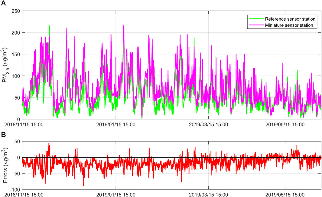
FIGURE 2. (A) Comparison of PM2.5 concentration measurements between the reference sensor station and the miniature sensor station; (B) Errors between the PM2.5 concentration measurements of the reference sensor station and the miniature sensor station. Figures are generated using Matlab (Version R2021b, https://www.mathworks.com/) [Software].
The measurement errors of miniature air quality monitors are susceptible to many external factors such as meteorological parameters and other non-conventional gaseous pollutant concentrations, and these external factors vary significantly from month to month. We categorize and summarize the measurement values of the reference sensor station and the miniature sensor station by month, and plot them into box plots for comparative analysis (Wang and Lu, 2006; Liu et al., 2021b). It can be seen from Figure 3 that the concentrations of PM2.5 are obviously different from month to month. The reference sensor station has the highest median measurement value of 72 μg/m3 in November, while the miniature sensor station also has the highest median measurement value of 94.61 μg/m3 in November. Due to the gradual decrease in temperature, high humidity, and low wind in the region in November, this meteorological condition makes it easier for airborne particles to accumulate and remain in the air, resulting in higher PM2.5 concentrations. The reference sensor station has the lowest median measurement value of 35 μg/m3 in May, while the miniature sensor station also has the lowest median measurement value of 36.47 μg/m3 in May. The region experienced lower humidity, higher temperatures, and sunny weather in May, which facilitated the dispersion and dilution of particulate matter, resulting in lower PM2.5 concentrations. In addition, the monthly average of the reference sensor station and the miniature sensor station have the largest error of −24.43 μg/m3 in January and the smallest error of −1.77 μg/m3 in May. The measurement errors are larger in the autumn and winter seasons and smaller in the spring and summer seasons, indicating that the measurement errors of the miniature air quality monitor have a certain relationship with the seasons and meteorological conditions.
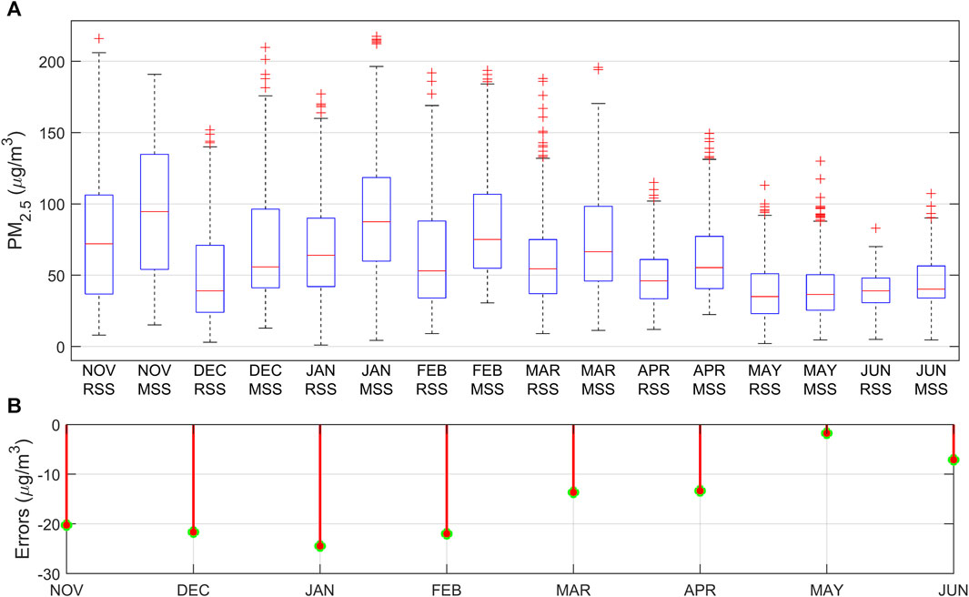
FIGURE 3. (A) Comparison of PM2.5 concentration measurements between the Reference Sensor Station (RSS) and the Miniature Sensor Station (MSS) on a monthly basis; (B) Comparison of errors for PM2.5 concentration measurements between the RSS and the MSS on a monthly basis.
Pearson correlation coefficient is employed by us to quantitatively portray the correlation between air pollutant concentrations and meteorological parameters (Resquin et al., 2021; Yang and Zhao, 2023). Equation 1 is its expression, where
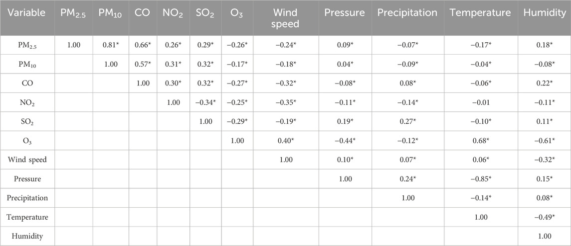
TABLE 2. Pearson linear correlation coefficient between the concentrations of six types of air pollutants measured at reference sensor station and five meteorological parameters measured at miniature sensor station (Band * indicates significant correlation at a significant level of 0.05).
A matrix color block diagram is a graphical form that visually displays data in different colors or areas based on their value size. In Figure 4, which is a matrix color block diagram of the variables, the larger the area of the circle, the stronger the correlation between the variables, and the smaller the area of the circle, the weaker the correlation between the variables. Darker colours of the circular blocks indicate negative correlation and lighter colours indicate positive correlation, and the correlation coefficient gradually increases as the colour of the block becomes lighter.

FIGURE 4. Pearson correlation coefficient matrix color block diagram between the concentration of two aerosols and four gases and climate factors.
Stepwise regression is an analytical method that introduces (or removes) variables into (or from) a regression equation one by one, according to the significance of the effect of the explanatory variables on the explained variables. In the case of multivariate screening of important variables, the use of stepwise regression analysis is a better way of avoiding multicollinearity between explanatory variables and eliminates the need for a heavy variable screening process (Duan et al., 2022).
Equations 2, 3 are the linear overall regression model containing
The stepwise regression method introduces (excludes) the independent variables with the criterion of maximum (minimum) partial regression sum of squares. In the introduction (exclusion) step, assuming that the model already contains
Support vector regression is based on the support vector machine model. It is an algorithm that achieves the optimal generalization ability of the model with less information about the samples, and introduces a kernel function to find high-dimensional hypersurfaces to achieve the optimal solution (Vergara et al., 2013). Unlike traditional regression models, support vector regression assumes the construction of an interval band with a width of
Suppose the training set
It is solved by the Lagrange multiplier method, and its dual forms Eqs 9, 10 can be obtained by introducing the Lagrange function. The dot product operation in high dimensional space is used to make
The Taylor diagram was first proposed in 2001 by Karl E. Taylor, an American atmospheric scientist, as a graph for comparing the differences between several models or observations and a reference model. It provides an intuitive way to compare the strengths and weaknesses of various model performances. The scatter in the Taylor diagram represents the different models, the radial line represents the Pearson correlation coefficient, the dashed line represents the centered root mean square difference, and the horizontal and vertical axes represent the standard deviation. Equations 15, 16 are the expressions for centered root mean square difference and standard deviation, where
There are many factors that influence the concentrations of the two aerosols and four gases, and multiple linear regression modelling is often used to find a linear relationship between these influences and the concentrations of the two aerosols and four gases. The key to a multiple linear regression model is the choice of independent variables. Too much or too little selection of independent variables can adversely affect the stability and usefulness of the model. The commonly used methods of independent variable selection include forward selection, backward elimination and stepwise regression. Among them, stepwise regression is a widely respected method of independent variable selection (Liu et al., 2021d). The stepwise regression method combines the ideas of forward selection and backward elimination, where the choice of adding or deleting independent variables is made at each step based on statistical significance in order to progressively optimise the model.
We randomly select 70% of the 4,144 data samples as a training set to train the parameters and weights of the model, and the remaining 30% of the data is used as a test set to evaluate the generalization ability of the model after the model training is completed. The PM2.5 concentration measured by the reference sensor is used as the dependent variable, and the 11 variables measured by the miniature air quality monitor are used as the independent variables to build the SRA model for PM2.5 using SPSS 26. At the significant level α = 0.05, the miniature sensor measured the remaining 9 variables except SO2 and O3 are introduced into the SRA model, indicating that they all have a significant effect on the PM2.5 concentration reference value. The F-value of the SRA model for PM2.5 is 2916.4, corresponding to a probability p-value of 0.000, indicating that the variables introduced into the model have a significant effect on the reference value of PM2.5 concentration as a whole. The Coefficient of Determination of the model is 0.901, indicating that 90.1% of the total variation in the dependent variable can be explained by the regression model (Xiang et al., 2023). Similarly, the SRA model results for the other five pollutants are shown in Table 3.
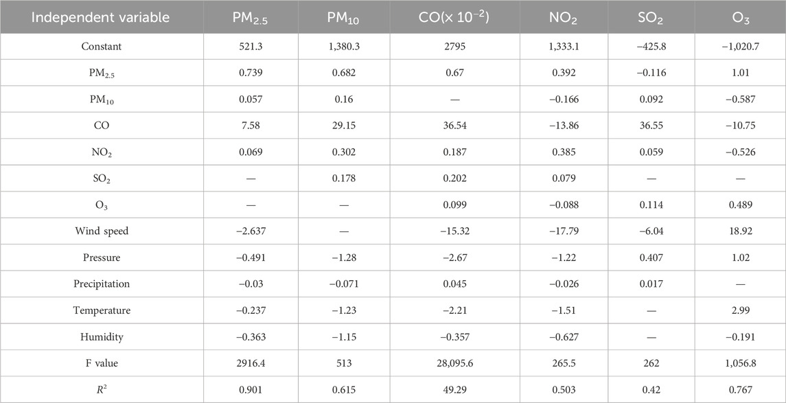
TABLE 3. Stepwise regression analysis model of six types of air pollutant concentrations. In the model, the dependent variable is the concentration of the six pollutants at the reference sensor station, and the independent variables are the measurements of the miniature sensor station (”—” represents the variables eliminated in the model).
Figure 5 demonstrates the effect of the SRA model for PM2.5 on the calibration of the measured data from the miniature air quality monitor. It can be seen that the miniature sensor measurement error is concentrated in [−40, 20], while the residuals of the SRA model are concentrated in [−20, 20]. In addition, the residuals of the SRA model are randomly concentrated near the zero point regardless of the training and test sets, indicating that the SRA model can satisfy the requirements for the error term. The residuals of the SRA model perform consistently in the test set and the training set, indicating that the model has good generalization ability.
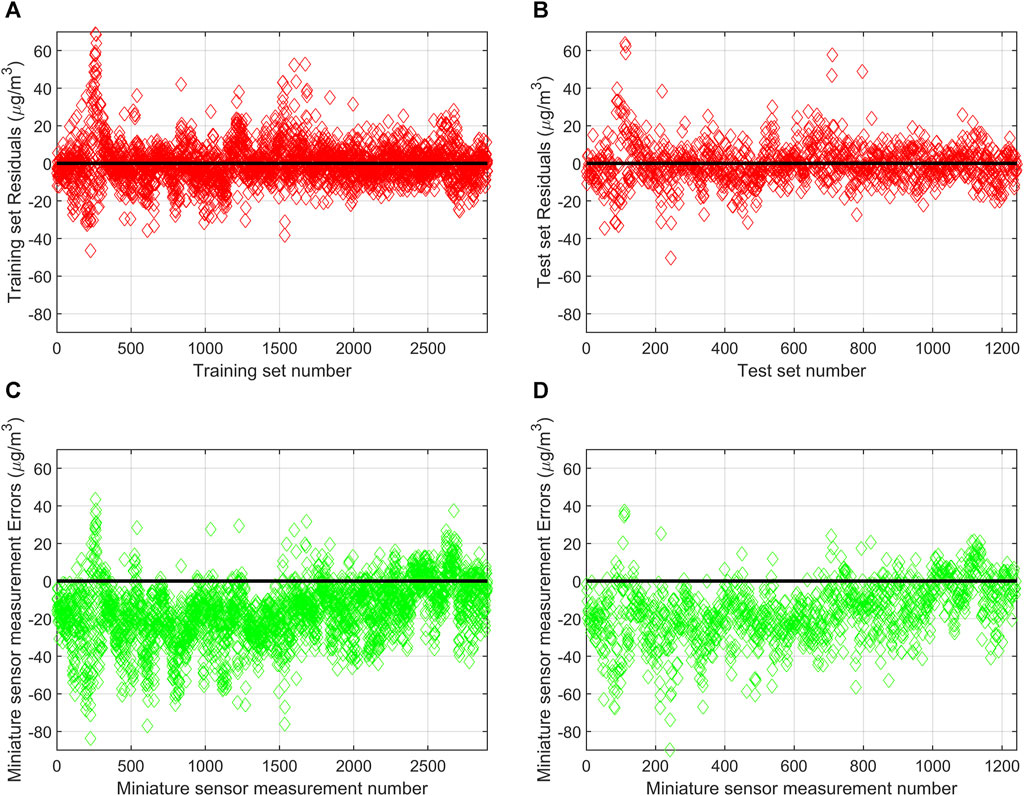
FIGURE 5. (A) Residuals of the SRA calibration model on the training set; (B) Residuals of the SRA calibration model on the test set; (C) The measurement error of the miniature sensor at the number corresponding to the training set of the SRA calibration model; (D) The measurement error of the miniature sensor at the number corresponding to the test set of the SRA calibration model.
The SRA model has extracted linear relationships between the two aerosols and four gases and the various influencing factors. However, the factors affecting the concentration of pollutants are very complex and there are still some non-linear relationships hidden in the residuals (Liu and Li, 2015). The SVR model has strong nonlinear modelling capability, robustness, ability to adapt to high dimensional data and also performs well in small sample situations. It is used in this study to find the nonlinear relationship between the six types of pollutants and the influencing factors.
The residuals of the SRA model for PM2.5 are used as response variables, the data measured by the miniature sensor are used as predictor variables, and the SVR model for residual calibration of six pollutants is built using the regression learner in Matlab. The default 5-fold cross-validation of the software is used in the experiments to prevent the SVR model from overfitting. The original dataset is divided into five equal-sized subsets, and from these five subsets, one of them is selected as the validation set and the remaining four subsets are used as the training set. The model is trained on the training set and the performance is evaluated using the RMSE on the validation set. Repeat the previous steps until each subset is used as a validation set and calculated to get five performance evaluations. Averaging these five performance evaluation results gives the final average performance evaluation result of the model.
The SVR model in the regression learner has three main parameters, box constraint mode, epsilon mode and kernel scale mode. The box constraint controls the penalty imposed on observations with large residuals. A larger box constraint gives a more flexible model. A smaller value gives a more rigid model, less sensitive to overfitting. Prediction errors that are smaller than the epsilon value are ignored and treated as equal to zero. A smaller epsilon value gives a more flexible model. The kernel scale controls the scale of the predictors on which the kernel varies significantly. A smaller kernel scale gives a more flexible model. For the kernel function mainly include linear kernel, quadratic kernel, cubic kernel and Gaussian kernel.
The selection of the three parameters is set to automatic and the software uses a heuristic procedure to automatically assign values to them. For the selection of the kernel function, it is determined by comparing the performance of each kernel function in the validation set. Finally, the Box constraint mode, Epsilon mode and Kernel scale mode of the SVR model for PM2.5 are set to 7.6, 0.76 and 0.83 respectively, and the kernel function is determined as Gaussian kernel. The final output of the combined SRA-SVR model for PM2.5 is obtained by adding the residual calibration values of the output values of the SVR model to the output values of the SRA model. The SRA-SVR combined calibration models for the other five pollutants can be obtained similarly.
In order to measure the regression effect of the SRA-SVR combined model for PM2.5, a one-dimensional linear regression model is established for PM2.5 concentration measured by the reference sensor as the independent variable and the output value of the SRA-SVR combined model as the dependent variable. As can be seen from Figure 6, the regression of the SRA-SVR combination model performs well in both the training set and the test set, indicating that the model has a strong generalization ability. The correlation coefficients between the output values of the SRA-SVR combined model and the target values are all greater than 0.96, and the regression coefficients of the two regression models are close to 1, which indicates that the output values of the SRA-SVR combined model are very close to the measured values of the reference sensor.
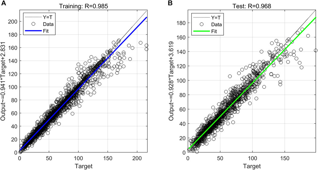
FIGURE 6. (A) The fitting effect of PM2.5’s SRA-SVR model on the training set; (B) The calibration effect of PM2.5’s SRA-SVR model on the test set.
Figure 7 shows the residual test plot of the SRA-SVR combined model for PM2.5. It can be seen that a total of 3,746 residuals are located in [−10, 10], accounting for 90.4%, a total of 4,052 residuals are located in [−20, 20], accounting for 97.78%, and only 13 residuals have an absolute value over 40, accounting for 0.31%. In the test set, a total of 1,044 residuals are located in [−10, 10], accounting for 83.99%, a total of 1,208 residuals are located in [−20, 20], accounting for 97.18%, and only 6 residuals have an absolute value over 40, accounting for 0.48%. Overall, the residuals roughly follow a normal distribution and are randomly and symmetrically distributed around the value of zero.
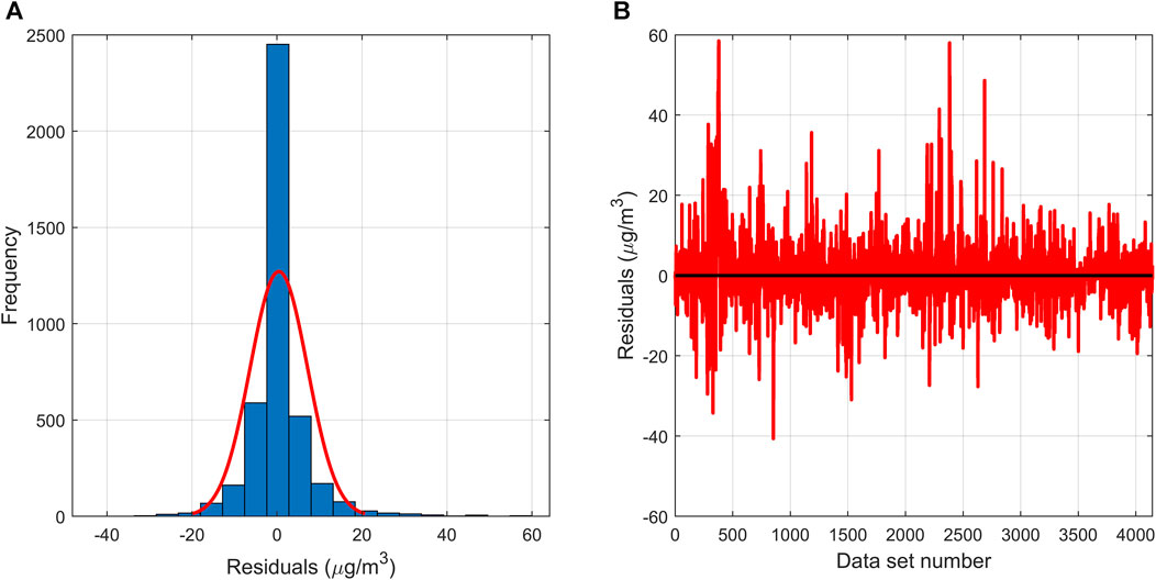
FIGURE 7. (A) The residual histogram of the SRA-SVR model; (B) The residual plot of the SRA-SVR model.
The SRA-SVR combined model enables calibration of PM2.5 concentrations measured by the miniature air quality monitor. In addition, separate SRA or SVR models, as well as models such as Decision Tree Regression (DTR) and multilayer perceptron neural network can also be implemented to calibrate PM2.5 concentrations measured by the miniature air quality monitor (Abdullah et al., 2020; Resquin et al., 2021; Balogun and Tella, 2022). The calibration effects for the models are measured by their performance on the training and test sets. In order to visualize the performance of each model, Taylor diagrams are used in this study to complete the comparison of each model.
As can be seen in Figure 8, the SRA and SVR models alone, as well as models such as DTR and MLP, enable the calibration of PM2.5 concentrations measured by the miniature air quality monitor. In the training set, SRA and MLP can achieve fitting to the data but the accuracy needs to be improved, DTR and SVR have high fitting accuracy to the data, and the SRA-SVR combination model given in this study has the strongest ability to fit the data. Comparing the performance of different models in the training set can provide some preliminary information about model performance and fitting ability. However, evaluating models based on performance in the training set alone is not sufficient. In order to more accurately evaluate model performance, it is critically necessary to evaluate model performance in the test set. It can be seen that in the test set, SRA, MLP and DTR models can achieve the prediction of the data, but the accuracy needs to be improved, the SVR and SRA-SVR combined models have a stronger prediction of the data. No matter the training set or test set, the SRA-SVR combined model performs the best compared to other given models.
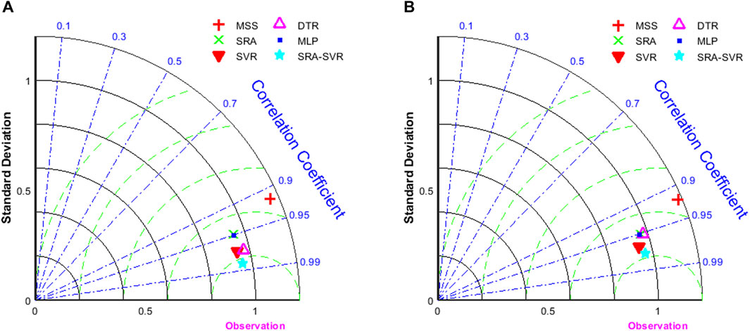
FIGURE 8. (A) Taylor diagram of the fitted PM2.5 concentration values for the five calibration models on the training set; (B) Taylor diagram of the calibrated PM2.5 concentration values for the five calibration models on the test set. Here MSS represents the measured values of the miniature sensor station on the corresponding set.
The SRA-SVR combined model has a good calibration for PM2.5 concentrations measured by the miniature sensors, and it needs to be evaluated whether it can also have a good calibration for other pollutants as well. MAE, MAPE and RMSE are used in this study to quantitatively evaluate the performance of each model (Liu et al., 2017; Ratkovic et al., 2023). As can be seen in Tables 4–6, except for the MAPE of the SRA model for SO2, the miniature air quality monitor has the maximum of the rest of the indicators, indicating that its measurements need to be calibrated. The SRA-SVR combined model proposed in this study has the best performance in all evaluation indicators. For the MAE indicator, the SRA-SVR models for CO and PM10 perform best on the training set and test set, respectively, with 92.1% and 80.87% improvement in accuracy, respectively. For the MAPE indicator, the SRA-SVR model for O3 performs best on the training and test sets with 95.13% and 87.43% improvement in accuracy, respectively. For the RMSE indicator, the SRA-SVR models for CO and SO2 perform best on the training set and test set, respectively, with 87.26% and 78.64% improvement in accuracy, respectively.
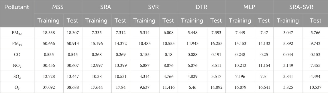
TABLE 4. The MAE of miniature sensor station and various air quality calibration models, in which reference sensor station is used as comparison object.
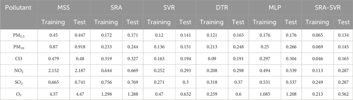
TABLE 5. The MAPE of miniature sensor station and various air quality calibration models, in which reference sensor station is used as comparison object.
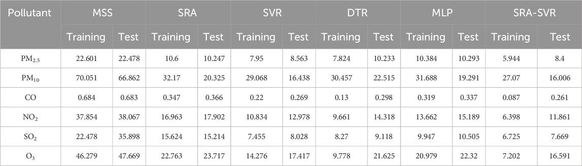
TABLE 6. The RMSE of miniature sensor station and various air quality calibration models, in which reference sensor station is used as comparison object.
In the current context of increasingly serious environmental problems, monitoring and assessment of air quality has become increasingly important. Miniature air quality monitors, as a rapid, real-time monitoring tool, are important for environmental protection, public health and urban planning in terms of their accuracy and reliability. However, its measurement accuracy needs to be improved for various reasons. The SRA-SVR combined model proposed in this study successfully improves its measurement accuracy by 61.33%–87.43%. This is very helpful for the development and promotion of miniature air quality monitors to ensure the sustainability of air quality. The SRA-SVR combined model has both the interpretability of the SRA model and the high accuracy of the SVR model, and it has been empirically demonstrated that the accuracy of this combined model is better than that of a single model. The SRA-SVR combined model is based on a study of 4,144 data sets for a total of 206 days in the time period from November 2018 to June 2019, covering four seasons across years. This indicates that the model is able to maintain strong stability across time periods and seasons. By comparing the experimental results of the training and test sets, the SRA-SVR combination model proposed in this study has a strong generalization ability. This further validates the scientific value and practical application prospects of calibrating miniature air quality monitors using the SRA-SVR model. However, factors such as climatic conditions, geographic features and population density in different regions may have an impact on air quality. Although the SRA-SVR combined model showed better performance in this study, its applicability to other regions still needs to be verified in practice. Further studies may consider expanding the sample coverage and incorporating other environmental factors to further validate and refine the applicability of the model.
The original contributions presented in the study are included in the article/Supplementary Material, further inquiries can be directed to the corresponding author.
XW: Writing–original draft, Writing–review and editing.
The author(s) declare that financial support was received for the research, authorship, and/or publication of this article. This research is supported by the Intelligent Manufacturing College, Sanmenxia Polytechnic.
The author declares that the research was conducted in the absence of any commercial or financial relationships that could be construed as a potential conflict of interest.
All claims expressed in this article are solely those of the authors and do not necessarily represent those of their affiliated organizations, or those of the publisher, the editors and the reviewers. Any product that may be evaluated in this article, or claim that may be made by its manufacturer, is not guaranteed or endorsed by the publisher.
The Supplementary Material for this article can be found online at: https://www.frontiersin.org/articles/10.3389/fenvs.2024.1348794/full#supplementary-material
DTR, Decision Tree Regression; MAE, Mean Absolute Error; MAPE, Mean Absolute Percentage Error; MLP, MultiLayer Perceptron neural network; RMSE, Root Mean Square Error; SRA, Stepwise Regression Analysis; SVR, Support Vector Regression.
Abdullah, S., Napi, NNLM, Ahmed, A. N., Mansor, W. N. W., Ramly, Z. T. A., Ismail, M., et al. (2020). Development of multiple linear regression for particulate matter (PM10) forecasting during episodic transboundary haze event in Malaysia. Atmosphere 1 (3), 289. doi:10.3390/atmos11030289
Akimoto, H. (2004). Akimoto H. Global air quality and pollution. Science 302, 1716–1719. doi:10.1126/science.1092666
Ayers, G. P. (2001). Comment on regression analysis of air quality data. Atmos. Environ. 35 (13), 2423–2425. doi:10.1016/S1352-2310(00)00527-6
Azid, A., Amran, M. A., Samsudin, M. S., Abd Rani, N. L., Khalit, S. I., Gasim, M. B., et al. (2018). Assessing indoor air quality using chemometric models. Pol. J. Environ. Stud. 27 (6), 2443–2450. doi:10.15244/pjoes/78154
Balogun, A. L., and Tella, A. (2022). Modelling and investigating the impacts of climatic variables on ozone concentration in Malaysia using correlation analysis with random forest, decision tree regression, linear regression, and support vector regression. Chemosphere 299, 134250. doi:10.1016/j.chemosphere.2022.134250
Brauer, M., Amann, M., Burnett, R. T., Cohen, A., Dentener, F., Ezzati, M., et al. (2012). Exposure assessment for estimation of the global burden of disease attributable to outdoor air pollution. Environ. Sci. Technol. 46 (2), 652–660. doi:10.1021/es2025752
Castell, N., Dauge, F. R., Schneider, P., Vogt, M., Lerner, U., Fishbain, B., et al. (2017). Can commercial low-cost sensor platforms contribute to air quality monitoring and exposure estimates? Environ. Int. 99, 293–302. doi:10.1016/j.envint.2016.12.007
Deo, R. C., Wen, X., and Qi, F. (2016). A wavelet-coupled support vector machine model for forecasting global incident solar radiation using limited meteorological dataset. Appl. Energy 168, 568–593. doi:10.1016/j.apenergy.2016.01.130
Ding, H. J., Liu, J. Y., Zhang, C. M., and Wang, Q. (2020). Predicting optimal parameters with random forest for quantum key distribution. Quantum Inf. Process 19 (2), 60–68. doi:10.1007/s11128-019-2548-3
Duan, Y., Xie, E., Liu, C., and Deng, J. (2022). Establishment of a combined diagnostic model of abdominal aortic aneurysm with random forest and artificial neural network. Atmosphere 13, 1371. doi:10.21203/rs.3.rs-864615/v1
Dun, M., Xu, Z., Chen, Y., and Wu, L. (2020). Short-term air quality prediction based on fractional grey linear regression and support vector machine. Math. Probl. Eng. 2020, 1–13. doi:10.1155/2020/8914501
Elangasinghe, M. A., Singhal, N., Dirks, K. N., Salmond, J. A., and Samarasinghe, S. (2014). Complex time series analysis of PM10 and PM2.5 for a coastal site using artifcial neural network modelling and k-means clustering. Atmos. Environ. 94, 106–116. doi:10.1016/j.atmosenv.2014.04.051
Jian, L., Zhao, Y., Zhu, Y., Zhang, M., and Bertolatti, D. (2012). An application of ARIMA model to predict submicron particle concentrations from meteorological factors at a busy roadside in Hangzhou, China. Sci. Total Environ. 426, 336–345. doi:10.1016/j.scitotenv.2012.03.025
Kaminska, J. A. (2018). The use of random forests in modelling short-term air pollution effects based on traffic and meteorological conditions: a case study in Wrocław. J. Environ. Manage 217, 164–174. doi:10.1016/j.jenvman.2018.03.094
Koo, J. W., Wong, S. W., Selvachandran, G., Long, H. V., and Son, L. (2019). Prediction of Air Pollution Index in Kuala Lumpur using fuzzy time series and statistical models. Air Qual. Atmos. Health 13, 77–88. doi:10.1007/s11869-019-00772-y
Liu, B., Jin, Y., and Li, C. (2021b). Analysis and prediction of air quality in Nanjing from autumn 2018 to summer 2019 using PCR-SVR-ARMA combined model. Sci. Rep-UK 11, 348. doi:10.1038/s41598-020-79462-0
Liu, B., Tan, X., Jin, Y., and Li, C. (2021c). Application of RR-XGBoost combined model in data calibration of micro air quality detector. Sci. Rep-UK 11, 15662. doi:10.1038/s41598-021-95027-1
Liu, B., Yu, W., Wang, Y., Lv, Q., and Li, C. (2021a). Research on data correction method of micro air quality detector based on combination of partial least squares and random forest regression. IEEE Access 9, 99143–99154. doi:10.1109/ACCESS.2021.3096216
Liu, B., Zhao, Q., Jin, Y., Shen, J., and Li, C. (2021d). Application of combined model of stepwise regression analysis and artificial neural network in data calibration of miniature air quality detector. Sci. Rep-UK 11, 3247. doi:10.1038/s41598-021-82871-4
Liu, B. C., Binaykia, A., Chang, P. C., Tiwari, M. K., and Tsao, C. C. (2017). Urban air quality forecasting based on multi-dimensional collaborative Support Vector Regression (SVR): a case study of Beijing-Tianjin-Shijiazhuang. Plos One 12 (7), e0179763. doi:10.1371/journal.pone.0179763
Liu, D. J., and Li, L. (2015). Application study of comprehensive forecasting model based on entropy weighting method on trend of PM2.5 concentration in Guangzhou, China. Int. J. Environ. Res. Pub He 12 (6), 7085–7099. doi:10.3390/ijerph120607085
Liu, Q., Liu, Y., Yang, Z., Zhang, T., and Zhong, Z. (2014). Daily variations of chemical properties in airborne particulate matter during a high pollution winter episode in Beijing. Acta Sci. Circumst. 34 (1), 12–18.
Luo, H., Tang, X., Wu, H., Kong, L., Wu, Q., Cao, K., et al. (2022). The impact of the numbers of monitoring stations on the national and regional air quality assessment in China during 2013–18. Adv. Atmos. Sci. 39 (10), 1709–1720. doi:10.1007/s00376-022-1346-5
Masson, N., Piedrahita, R., and Hannigan, M. (2015). Approach for quantification of metal oxide type semiconductor gas sensors used for ambient air quality monitoring. Sens. Actuat B-chem. 208, 339–345. doi:10.1016/j.snb.2014.11.032
Oettl, D., Almbauer, R. A., Sturm, P. J., and Pretterhofer, G. (2003). Dispersion modelling of air pollution caused by road traffic using a Markov chain–Monte Carlo model. Stoch. Env. Res. Risk A 17, 58–75. doi:10.1007/s00477-002-0120-6
Poloniecki, J. D., Atkinson, R. W., Deleon, A. P., and Anderson, H. R. (1997). Daily time series for cardiovascular hospital admissions and previous day's air pollution in London, UK. Occup. Environ. Med. 54 (8), 535–540. doi:10.1136/oem.54.8.535
Ratkovic, K., Kovac, N., and Simeunovic, M. (2023). Hybrid LSTM model to predict the level of air pollution in Montenegro. Appl. Sci-Basel. 13, 10152. doi:10.3390/app131810152
Reich, S. L., Gomez, D. R., and Dawidowski, L. E. (1999). Artificial neural network for the identification of unknown air pollution sources. Atmos. Environ. 33 (18), 3045–3052. doi:10.1016/S1352-2310(98)00418-X
Resquin, M. D., Lichtig, P., Alessandrello, D., Dawidowski, L., Gómez, D., Rössler, C., et al. (2021). A machine learning approach to address air quality changes during the covid-19 lockdown in Buenos Aires, Argentina. Earth Syst. Sci. Data 15, 189–209. doi:10.5194/essd-2021-318
Spinelle, L., Gerboles, M., Villani, M. G., Aleixandre, M., and Bonavitacola, F. (2015). Field calibration of a cluster of low-cost available sensors for air quality monitoring. part A: ozone and nitrogen dioxide. Sens. Actuat B-chem. 215, 249–257. doi:10.1016/j.snb.2015.03.031036
Sun, W., Zhang, H., Palazoglu, A., Singh, A., Zhang, W. D., and Liu, S. W. (2013). Prediction of 24-hour-average PM2.5 concentrations using a hidden Markov model with different emission distributions in Northern California. Sci. Total Environ. 443, 93–103. doi:10.1016/j.scitotenv.2012.10.070
Suriano, D., Cassano, G., and Penza, M. (2020). Design and development of a flexible, plug-and-play, cost-effective tool for on-field evaluation of gas sensors. J. Sensors 2020, 1–20. doi:10.1155/2020/8812025
Tagaris, E., Manomaiphiboon, K., Liao, K. J., Leung, L. R., Woo, J. H., He, S., et al. (2007). Impacts of global climate change and emissions on regional ozone and fine particulate matter concentrations over the United States. J. Geophys. Res-Atmos. 112, D14312. doi:10.1029/2006JD008262
Tai, A. P. K., Mickley, L. J., and Jacob, D. J. (2010). Correlations between fine particulate matter (PM2.5) and meteorological variables in the United States: implications for the sensitivity of PM2.5 to climate change. Atmos. Environ. 44 (32), 3976–3984. doi:10.1016/j.atmosenv.2010.06.060
Vergara, A., Fonollosa, J., Mahiques, J., Trincavelli, M., Rulkov, N., and Huerta, R. (2013). On the performance of gas sensor arrays in open sampling systems using inhibitory support vector machines. Sens. Actuat B-chem. 185, 462–477. doi:10.1016/j.snb.2013.05.027
Wang, X., and Lu, W. (2006). Seasonal variation of air pollution index: Hong Kong case study. Chemosphere 63 (8), 1261–1272. doi:10.1016/j.chemosphere.2005.10.031
Wang, Z., Feng, J., Fu, Q., Gao, S., Chen, X., and Cheng, J. (2019). Quality control of online monitoring data of air pollutants using artificial neural networks. Air Qual. Atmos. Hlth 12 (10), 1189–1196. doi:10.1007/s11869-019-00734-4
Wu, H., Liu, S., Du, J., and Fang, Z. (2022). A novel grey spatial extension relational model and its application to identify the drivers for ambient air quality in Shandong Province, China. Sci. Total Environ. 845, 157208. doi:10.1016/j.scitotenv.2022.157208
Xiang, X., Fahad, S., Han, M. S., Naeem, M. R., and Room, S. (2023). Air quality index prediction via multi-task machine learning technique: spatial analysis for human capital and intensive air quality monitoring stations. Air Qual. Atmos. Hlth 16 (1), 85–97. doi:10.1007/s11869-022-01255-3
Xu, Y., You, T., Wen, Y., Ning, J., Xiao, Y., and Shen, H. (2023). Air quality research based on B-Spline functional linear model: a case study of Fujian province, China. Appl. Sci-Basel. 13, 11206. doi:10.3390/app132011206
Yang, J., and Zhao, Y. (2023). Performance and application of air quality models on ozone simulation in China – a review. Atmos. Environ. 293, 119446. doi:10.1016/j.atmosenv.2022.119446
Yu, R., Yang, Y., Yang, L., Han, G., and Oguti, M. (2016). RAQ—a random forest approach for predicting air quality in urban sensing systems. Sensors 16, 86–104. doi:10.3390/s16010086
Keywords: statistical models, stepwise regression analysis, support vector regression, data calibration, pollutant concentration
Citation: Wang X (2024) Advancing sustainable air quality through calibration of miniature air quality monitors with SRA-SVR combined model. Front. Environ. Sci. 12:1348794. doi: 10.3389/fenvs.2024.1348794
Received: 03 December 2023; Accepted: 25 January 2024;
Published: 06 February 2024.
Edited by:
Kanhu Charan Pattnayak, National Environment Agency, SingaporeReviewed by:
Arti Choudhary, Utkal University, IndiaCopyright © 2024 Wang. This is an open-access article distributed under the terms of the Creative Commons Attribution License (CC BY). The use, distribution or reproduction in other forums is permitted, provided the original author(s) and the copyright owner(s) are credited and that the original publication in this journal is cited, in accordance with accepted academic practice. No use, distribution or reproduction is permitted which does not comply with these terms.
*Correspondence: Xiaofei Wang, d3hmXzEyMzQ1NkB5ZWFoLm5ldA==
Disclaimer: All claims expressed in this article are solely those of the authors and do not necessarily represent those of their affiliated organizations, or those of the publisher, the editors and the reviewers. Any product that may be evaluated in this article or claim that may be made by its manufacturer is not guaranteed or endorsed by the publisher.
Research integrity at Frontiers
Learn more about the work of our research integrity team to safeguard the quality of each article we publish.