Lightweight land cover classification via semantic segmentation of remote sensing imagery and analysis of influencing factors

Land cover classification is of great value and can be widely used in many fields. Earlier land cover classification methods used traditional image segmentation techniques, which cannot fully and comprehensively extract the ground information in remote sensing images. Therefore, it is necessary to integrate the advanced techniques of deep learning into the study of semantic segmentation of remote sensing images. However, most of current high-resolution image segmentation networks have disadvantages such as large parameters and high network training cost. In view of the problems above, a lightweight land cover classification model via semantic segmentation, DeepGDLE, is proposed in this paper. The model DeepGDLE is designed on the basis of DeeplabV3+ network and utilizes the GhostNet network instead of the backbone feature extraction network in the encoder. Using Depthwise Separable Convolution (DSC) instead of dilation convolution. This reduces the number of parameters and increases the computational speed of the model. By optimizing the dilation rate of parallel convolution in the ASPP module, the “grid effect” is avoided. ECANet lightweight channel attention mechanism is added after the feature extraction module and the pyramid pooling module to focus on the important weights of the model. Finally, the loss function Focal Loss is utilized to solve the problem of category imbalance in the dataset. As a result, the model DeepGDLE effectively reduces the parameters of the network model and the network training cost. And extensive experiments compared with several existing semantic segmentation algorithms such as DeeplabV3+, UNet, SegNet, etc. show that DeepGDLE improves the quality and efficiency of image segmentation. Therefore, compared to other networks, the DeepGDLE network model can be more effectively applied to land cover classification. In addition, in order to investigate the effects of different factors on the semantic segmentation performance of remote sensing images and to verify the robustness of the DeepGDLE model, a new remote sensing image dataset, FRSID, is constructed in this paper. This dataset takes into account more influences than the public dataset. The experimental results show that on the WHDLD dataset, the experimental metrics mIoU, mPA, and mRecall of the proposed model, DeepGDLE, are 62.29%, 72.85%, and 72.46%, respectively. On the FRSID dataset, the metrics mIoU, mPA, and mRecall are 65.89%, 74.43%, and 74.08%, respectively. For the future scope of research in this field, it may focus on the fusion of multi-source remote sensing data and the intelligent interpretation of remote sensing images.

1 Introduction

Land cover classification is of great value and can be widely used in many fields such as agricultural and forestry planning, urban and rural planning, meteorological changes, military, environmental protection, and biodiversity research. In recent years, with the continuous improvement of the observation capability of high-resolution satellites, the amount of high-resolution remote sensing image data has increased dramatically, and accurate and rapid segmentation and extraction of land cover information has become the focus of research in the field of remote sensing images (Shao et al., 2020). Semantic segmentation of remote sensing images refers to the assignment of each pixel point in a multispectral or hyperspectral remote sensing image to a different feature category for automatic feature identification and classification. The main goal of this technique is to segment the input remote sensing image into multiple regions and assign a semantic category label to each pixel. This pixel is then indicated to which object or region of the pixel belongs. Compared to traditional remote sensing image classification, semantic segmentation requires not only classifying the entire image, but also classifying each pixel point. Therefore, it has high level of accuracy and detail (Li et al., 2018).

Traditional image segmentation techniques include threshold-based segmentation (Cao et al., 2019), cluster-based segmentation (Li et al., 2021), and edge-based segmentation (Pan et al., 2021), several methods have their own advantages and disadvantages (Kaur, 2015). The greatest advantages for the three traditional methods are their relative simplicity and intuition, computational efficiency, ability to perform automated segmentation, and adaptability. But they have more disadvantages. There are problems such as over-sensitivity to light and noise, difficulty in handling complex textures and difficult shape conditions, and sensitivity to initial parameters. The advantages of these three methods cannot eliminate the effects of the disadvantages. Therefore, for remote sensing images with high spatial resolution, complex background and many targets, the traditional image segmentation methods cannot fully and comprehensively extract the information in remote sensing images and cannot achieve good segmentation results. So, there is a need to incorporate advanced techniques in deep learning for segmentation studies of remote sensing images.

The research gaps in the field of semantic segmentation of remote sensing images are mainly reflected in the aspects of data acquisition and processing, algorithms and models, evaluation criteria and methods, and application scenarios. For the research objectives in the field of semantic segmentation of remote sensing images, the main focus is on improving the segmentation accuracy, reducing the computational complexity, expanding the application scenarios, and promoting the intersection of disciplines.

In the early days Jonathan et al. (2015) proposed full convolutional neural networks (FCN). The model uses a fully convolutional layer instead of a fully connected layer, which greatly reduces the number of parameters and computation. It incorporates the features of the intermediate layer and accepts input images of arbitrary size, and is an end-to-end semantic segmentation on the basis of pixel level. Fu et al. (2017) used FCN to classify high-resolution remote sensing images. Yuan et al. (2021) used the PSPNet network to do land cover classification of high spatial resolution multispectral remote sensing images. Hou et al. (2021) utilized the UNet network to extract remote sensing roads. Weng et al. (2020) utilized SegNet network to segment the waters. The above research has made some contribution to remote sensing image segmentation, but there is still much room for improvement in terms of accuracy and other aspects.

The Deeplab (Chen et al., 2014) semantic segmentation family combines a deep convolutional neural network and a probabilistic graph model to increase the sensory field of the convolutional operation process and maintain the resolution through null convolution. This series proposes and improves Atrous Spatial Pyramid Pooling (ASPP) (Chen et al., 2018a). ASPP enables the full fusion of different levels of semantic information, combined with spatial convolution with different dilation rates (Chen et al., 2017). Therefore ASPP module can effectively capture scale information. DeeplabV3+ (Chen et al., 2018b) combines the advantages of the encoding-decoding structure and the ASPP module, and has a relatively good impact in the field of semantic segmentation. At this stage DeeplabV3+ has become a semantic segmentation algorithm with superior comprehensive performance. In terms of image information extraction, DeepLabV3+ has better segmentation results than commonly used segmentation models such as FCN and PSPNet Du et al. (2021) combined DeeplabV3+ and object-based image analysis for semantic segmentation of ultra-high resolution remote sensing images. Yao et al. (2021) utilized a lightweight DeeplabV3+ model on the basis of the attention mechanism for optical remote sensing image detection with overall better segmentation results.

However, the DeeplabV3+ model still has some shortcomings. First of all, the model complexity is high, its feature extraction network Xception (Chollet, 2017) has more network layers and large number of parameters. Moreover, the convolution method in the ASPP module is ordinary convolution, which does not reduce the number of parameters well. This makes the whole model deeper and more complex, and increases the requirements for hardware devices. This will lead to slower model convergence and reduce the speed of network training. Second, the extraction of feature information is not complete enough. The process of feature extraction at the coding end gradually reduces the spatial dimensions of the input data, resulting in the loss of useful information. The details of the features are not better restored at the time of decoding. Finally, low accuracy for target edge recognition. Although the ASPP module can improve the extraction ability of the model to the target boundary, it cannot completely simulate the connection between the local features of the target. This makes the target segmentation has a hollow phenomenon, and there are problems such as low recognition accuracy and poor edge recognition effect.

To address the problems above, and in order to achieve the research objective of being able to segment geographic information remote sensing images more accurately and efficiently, DeepGDLE (a lightweight land cover classification model via semantic segmentation on the basis of DeeplabV3+ accompanied with the GhostNet, DSC, Focal Loss, and ECANet) is proposed in this paper. The model is on the basis of DeeplabV3+ model, which replaces the backbone feature extraction network Xception with the lightweight GhostNet (Han et al., 2020) network to reduce the number of parameters and the memory footprint. Replacing all normal convolutions in the ASPP module with Depthwise Separable Convolution (DSC) reduces the number of parameters and computational cost, and lightens the model. Modifying the dilation rate of parallel convolution in the ASPP module to avoid the “grid effect”. The ECANet attention mechanism (Wang et al., 2020) is added after the feature extraction network module and the ASPP module, which effectively avoids the effect of dimensionality reduction on the learning effect of channel attention. And the accuracy of feature extraction is improved by the local cross-channel interaction strategy without dimensionality reduction. The semantic segmentation loss function, Focal Loss (Lin et al., 2017), is used to balance the weights of different dataset categories. The overall model ultimately improves the efficiency and accuracy of processing information, resulting in the training of more accurate segmentation models.

In summary, the main contributions of this paper include three aspects, which are listed as following.

(1) A new comprehensive model, DeepGDLE, for land cover classification via semantic segmentation is proposed, which is an improved model on the basis of DeeplabV3+, by introducing the advantages of GhostNet, DSC, Focal Loss, ECANet and other models. It can realize lighter weight and more accurate performance.

(2) The influences of some important factors to the performance of land cover classification were examined by extensive experiments using DeepGDLE. The factors include the main category in the image and its percentage, the shadow percentages in the image, the categories count in the image, and so on. The results of experiments also verified the robustness of DeepGDLE.

(3) A new dataset of remote sensing images with land cover information, FRSID (Fuyang Remote Sensing Image Dataset), is constructed and shared in this paper. The dataset meets the requirements of the robustness validation experiments of the DeepGDLE model. The dataset consists of 4,500 original maps as well as labeled maps, and there are eight classifications in the overall dataset: cropland, vegetation, building, water body, general road, parking lot, main road, and playground.

The rest of the paper is organized as follows. The second section details the main structure of the DeepGDLE model proposed in this paper and the basic principles involved. The third part describes the experimental environment and the specific program of the experiment, the experimental steps, and the collection and processing of the data set. The results of the experiments as well as the analysis of the results of the ablation comparison experiments are presented in the fourth section. Finally, Part V summarizes and looks forward to the work of this paper.

2 Materials and methods

2.1 Main ideas

In the traditional DeeplabV3+ model, the Xception network with a large number of parameters was used for the feature extraction network. Due to its excessive number of network layers and the use of ordinary convolution in the ASPP module after feature extraction, the complexity of the model is large. This leads to an increase in the difficulty of model training and can cause problems such as slower speed of network training and convergence. In addition, in the encoder part, the shallow network information is directly input to the decoder due to the loss of effective information caused by dimensionality reduction. This leads to poor edge segmentation between categories.

In order to improve the segmentation performance and training speed of the model, this paper proposes a lightweight network applied to high-resolution remote sensing image segmentation. It is improved on the basis of DeeplabV3+ network, DeepGDLE, is proposed in this paper. Its structure is shown in Figure 1. The overall methodology flow is shown in Figure 2.

FIGURE 1

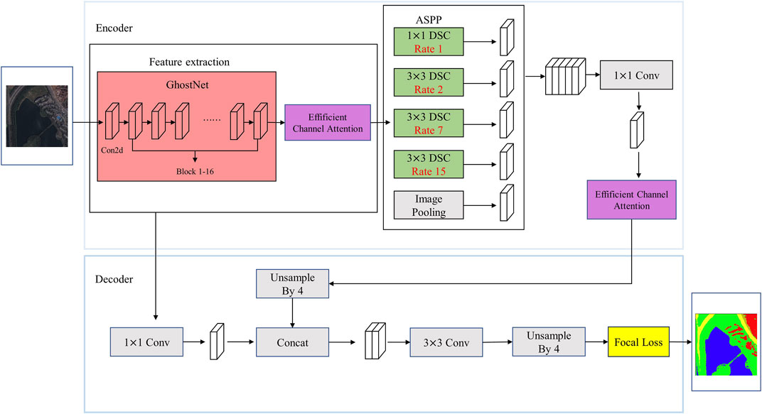
FIGURE 1. DeepGDLE model structure.

FIGURE 2

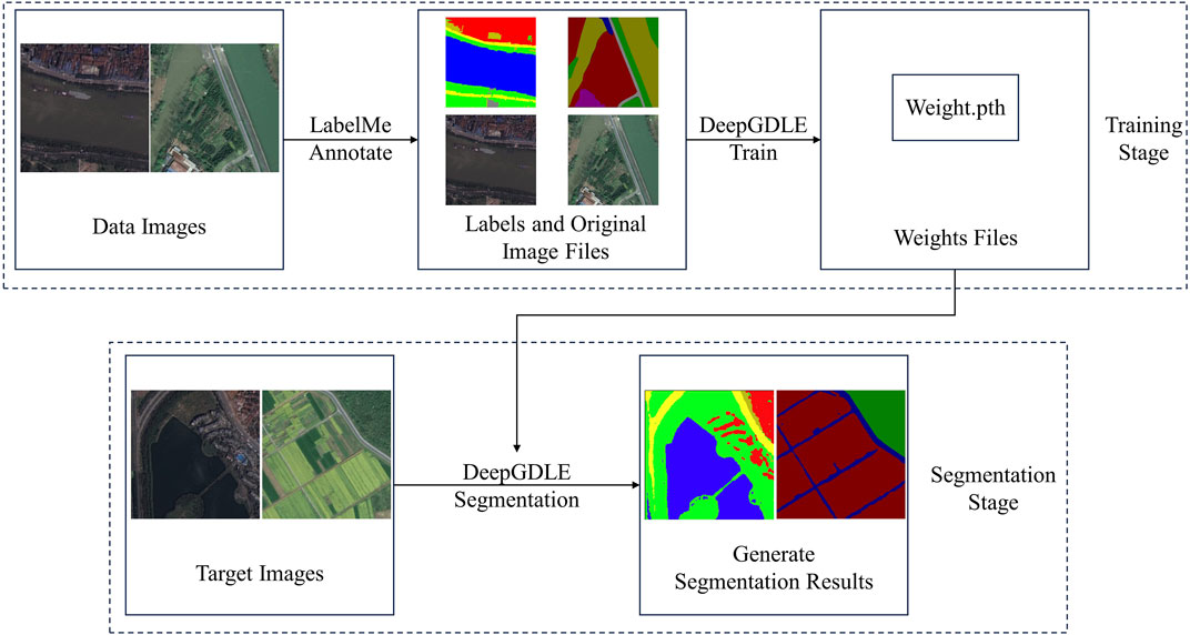
FIGURE 2. Methodology flow chart.

The main ideas of DeepGDLE proposed in this paper includes the following five aspects.

(1) Replacing Xception with GhostNet. On the basis of the DeeplabV3+ framework, the backbone feature extraction network Xception is replaced with the lightweight GhostNet network, which can significantly reduce the amount of parameter computation of the model, lower the memory occupation, and improve the computational speed of the model.

(2) Replacing normal convolution with Depthwise Separable Convolution (DSC). The ordinary convolution in the ASPP module is replaced with depthwise separable convolution to further reduce the number of parameters and computational cost of the model, and improve the computational speed of the model.

(3) Optimizing the dilation rate of parallel convolution in the ASPP module. When the dilation rate of the parallel cavity convolution is not set properly, it is easy to cause the “grid effect”. Therefore, the dilation rate in the original ASPP module was optimized, and the dilation rate with better results was selected after trying multiple dilation rates.

(4) Adding lightweight channel attention mechanism ECANet. Adding ECANet attention mechanism after the backbone feature extraction module and ASPP module. By utilizing appropriate cross-channel interactions, the impact of dimensionality reduction on the learning effect of channel attention is effectively avoided, and the accuracy of feature extraction is improved.

(5) Replacing the Cross Entropy Loss Function with Focal Loss. In order to reduce the impact of large differences in the proportion of feature categories on the accuracy of model feature classification, the Focal Loss is used to optimize the weights of the categories occupying different weights in the dataset, and to reduce the problems caused by data imbalance.

2.2 Replacing Xception with GhostNet

DeeplabV3+ is an improvement of the DeeplabV3 network, where the overall model replaces the underlying network with a residual network, adding a simple and effective encoder-decoder structure to optimize the segmentation results. On the coding side, DeeplabV3+ network utilizes Xception network to extract features from the input image. The image features are fused using ASPP module to avoid information loss. Where Xception is a deep convolutional neural network containing input, intermediate and output streams, and ASPP is a feature extraction module containing multiple multi-scale pyramids. Utilizing the ASPP structure to solve multiscale problems. Bilinear interpolation up-sampling is performed at the decoding end to improve the accuracy of network segmentation.

In this paper, the backbone feature extraction network of DeeplabV3+ is modified to the more lightweight GhostNet network. GhostNet has shallower network layers, fewer parameters, lower model complexity, and faster network training and convergence compared to Xception networks. Compared to lightweight networks such as MobileNet (Howard et al., 2017) and ShuffleNet (Zhang et al., 2018) on different datasets, GhostNet has the smallest parameter size, faster training speed and best training accuracy.

GhostNet consists of a bunch of Ghost bottlenecks, which are built on Ghost modules. The first layer is a standard convolutional layer with 16 convolutional kernels, followed by a series of Ghost bottlenecks with progressively more channels. These Ghost bottlenecks are categorized into different stages on the basis of their input feature map size. All Ghost bottlenecks are applied with stride = 1, except for the last Ghost bottleneck in each phase, which has stride = 2. Finally, the feature maps are converted into 1280-dimensional feature vectors for final classification using global average pooling and convolutional layers. The SE module is also used for residual layers in some Ghost bottlenecks. In contrast to MobileNetV3 (Howard et al., 2019), GhostNet swaps out the Hard-swish (Zoph and Le, 2017) activation function with the ReLU (Glorot et al., 2011) activation function.

There are two Ghost modules in a G-bneck module. The first of these Ghost module is used to increase the number of channels in the dilation layer, specifying the ratio between the number of output and input channels as the dilation ratio. The second Ghost module reduces the number of channels to match the channels in the shortcut branch. When the step size is 2, a deep convolutional layer with a step size of 2 is added between the two Ghost modules. The specific G-bneck module structure is shown in Supplementary Figure S1.

The GhostNet model consists of a stack of Ghost modules, G-bneck stands for Ghost Bottleneck. #exp stands for dilation size. #out stands for the number of output channels. SE indicates whether the SE module is used. Stride stands for the step size. The network structure is shown in Table 1.

TABLE 1

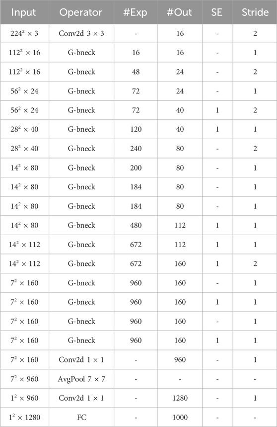
TABLE 1. GhostNet network model structure.

2.3 Replacing normal convolution with depthwise separable convolution

The main role of the convolutional layer is to perform feature extraction, where the input feature map is subjected to a convolution operation by the convolution kernel. The convolution kernel also learns the spatial and channel properties in the feature map. Depthwise Separable Convolution (DSC) adds a transition layer to the standard convolution process, decomposing it into Depthwise convolution (Tan and Le, 2019) and 1 × 1 point-by-point convolution (Guo et al., 2018), which is used to consider spatial correlation and channel correlation, respectively. Depthwise separable convolution divides it into two layers, one for filtering and one for combining. This decomposition process is able to drastically reduce the computational and parametric quantities of the model without losing much accuracy.

Assume that the size of the input feature map is ${\mathrm{D}}_{\mathrm{K}}\times {\mathrm{D}}_{\mathrm{K}}\times \mathrm{M}$ and the size of the convolution kernel is ${\mathrm{D}}_{\mathrm{F}}\times {\mathrm{D}}_{\mathrm{F}}\times \mathrm{M}$, and its number is $\mathrm{N}$. Assuming that a convolution operation is performed for each point in the spatial location of the corresponding feature map, a total of ${\mathrm{D}}_{\mathrm{K}}\times {\mathrm{D}}_{\mathrm{K}}\times {\mathrm{D}}_{\mathrm{F}}\times {\mathrm{D}}_{\mathrm{F}}\times \mathrm{M}$ computations are required for a single convolution, as shown in Supplementary Figure S2 for the standard convolution operation process. The spatial dimension of the feature map consists of a total of ${\mathrm{D}}_{\mathrm{K}}\times {\mathrm{D}}_{\mathrm{K}}$ points, while the computation of the convolution operation for each point is the same as the size of the convolution kernel, which is ${\mathrm{D}}_{\mathrm{F}}\times {\mathrm{D}}_{\mathrm{F}}\times \mathrm{M}$. As shown in Supplementary Figures S3, S4, the process of depthwise separable convolution operation is shown. Supplementary Figure S3 shows the deep convolution process, Supplementary Figure S4 shows the point-by-point convolution process. The calculation of the formula is derived from the article published in CVPR by (Howard et al., 2017) in 2017.

So, for a single convolution, the total amount of computation is as follows. Where ${\mathrm{D}}_{\mathrm{K}}$ denotes the height and width of the convolution kernel, ${\mathrm{D}}_{\mathrm{F}}$ denotes the depth of the input feature map, which is the number of channels contained in the input feature map, $\mathrm{M}$ denotes the number of channels included in the feature map. Details as shown in Eq. 1.

${\mathrm{D}}_{\mathrm{K}}\times {\mathrm{D}}_{\mathrm{K}}\times {\mathrm{D}}_{\mathrm{F}}\times {\mathrm{D}}_{\mathrm{F}}\times \mathrm{M}(1)$

For N convolutions, the total number of computations is as shown in Eq. 2.

${\mathrm{D}}_{\mathrm{K}}\times {\mathrm{D}}_{\mathrm{K}}\times {\mathrm{D}}_{\mathrm{F}}\times {\mathrm{D}}_{\mathrm{F}}\times \mathrm{M}\times \mathrm{N}(2)$

In depthwise separable convolution, for depth convolution, the computation is as shown in Eq. 3.

${\mathrm{D}}_{\mathrm{K}}\times {\mathrm{D}}_{\mathrm{K}}\times {\mathrm{D}}_{\mathrm{F}}\times {\mathrm{D}}_{\mathrm{F}}\times \mathrm{M}\times \mathrm{N}(3)$

For point-by-point convolution, the computation is as shown in Eq. 4.

${\mathrm{D}}_{\mathrm{K}}\times {\mathrm{D}}_{\mathrm{K}}\times \mathrm{M}\times \mathrm{N}(4)$

So, for one depthwise separable convolution, the total amount of computation is as shown in Eq. 5.

${\mathrm{D}}_{\mathrm{K}}\times {\mathrm{D}}_{\mathrm{K}}\times {\mathrm{D}}_{\mathrm{F}}\times {\mathrm{D}}_{\mathrm{F}}\times \mathrm{M}+{\mathrm{D}}_{\mathrm{K}}\times {\mathrm{D}}_{\mathrm{K}}\times \mathrm{M}\times \mathrm{N}(5)$

The ratio of the computational effort of the depthwise separable convolution with respect to the ordinary convolution is as shown in Eq. 6.

$\frac{{\mathrm{D}}_{\mathrm{K}}\times {\mathrm{D}}_{\mathrm{K}}\times {\mathrm{D}}_{\mathrm{F}}\times {\mathrm{D}}_{\mathrm{F}}\times \mathrm{M}+{\mathrm{D}}_{\mathrm{K}}\times {\mathrm{D}}_{\mathrm{K}}\times \mathrm{M}\times \mathrm{N}}{{\mathrm{D}}_{\mathrm{K}}\times {\mathrm{D}}_{\mathrm{K}}\times {\mathrm{D}}_{\mathrm{F}}\times {\mathrm{D}}_{\mathrm{F}}\times \mathrm{M}\times \mathrm{N}}=\frac{1}{\mathrm{N}}+\frac{1}{{\mathrm{D}}_{\mathrm{F}}\times {\mathrm{D}}_{\mathrm{F}}}(6)$

2.4 Optimizing the dilation rate in the ASPP module

In the ASPP module, if the dilation rate of the parallel cavity convolution is not properly chosen, the “grid effect” (Wang et al., 2018) will easily occur, which interferes with the accuracy of the model segmentation. For the encoding part, the use of dilated convolute on can expand the sense field and reduce the use of downsampling, but it will lead to a more serious loss of detail in the downsampling.

The goal of optimizing the dilation rate is to have the final feeler field fully cover the entire region without any voids or missing edges. Define the maximum distance between two non-zero points as follows. where ${\mathrm{M}}_{\mathrm{i}}$ denotes the size (width or height) of the ith layer of the feature map, ${\mathrm{r}}_{\mathrm{i}}$ denotes the radius size of the convolution kernel corresponding to the feature map of the ith layer. Details as shown in Eq. 7.

${\mathrm{M}}_{\mathrm{i}}=\max \left[{\mathrm{M}}_{\mathrm{i}+1}-2{\mathrm{r}}_{\mathrm{i}},{\mathrm{M}}_{\mathrm{i}+1}-2\left({\mathrm{M}}_{\mathrm{i}+1}-{\mathrm{r}}_{\mathrm{i}}\right),{\mathrm{r}}_{\mathrm{i}}\right](7)$

In the formula, ${\mathrm{M}}_{\mathrm{n}}={\mathrm{r}}_{\mathrm{n}}$ and the goal is to have ${\mathrm{M}}_2\le \mathrm{K}$.

For a common dilated convolutional kernel size $\mathrm{K}=3$, if $\mathrm{r}=\left[1,2,5\right]$, the Eq. 8 can be obtained.

${\mathrm{M}}_2=\max \left[{\mathrm{M}}_3-2{\mathrm{r}}_2,-{\mathrm{M}}_3+2{\mathrm{r}}_2,{\mathrm{r}}_2\right]=\max \left[1,-1,2\right]=2(8)$

At this point, ${\mathrm{M}}_2=2\le \mathrm{K}=3$, which satisfies the objective. The schematic diagram of the design is represented in Supplementary Figure S5.

If $\mathrm{r}=\left[1,2,9\right]$. The Eq. 9 can be obtained.

${\mathrm{M}}_2=\max \left[{\mathrm{M}}_3-2{\mathrm{r}}_2,-{\mathrm{M}}_3+2{\mathrm{r}}_2,{\mathrm{r}}_2\right]=\max \left[5,-5,2\right]=5(9)$

At this point, ${\mathrm{M}}_2=5>\mathrm{K}=3$, which does not satisfy the objective. The schematic diagram of the design is represented in Supplementary Figure S6.

The dilation convolution strategy using different dilation rates is given as a form of sawtooth wave variation. Sawtooth wave can fulfill the segmentation requirements for both small and large objects. Convolution within a group should not have a fixed transform factor. Therefore, conventions greater than 1 should not be used, otherwise there is no way to reduce the grid effect. A dilation rate of the same or equal proportions loses a lot of information, and a dilation rate of a sawtooth waveform covers a much larger area while the parameters remain unchanged.

2.5 Adding lightweight channel attention mechanism ECANet

In the field of deep learning, the attention mechanism focuses on significant feature differences, extracting from a large number of data features to select the information that is more important for the task at hand.

Common attention mechanisms include channel attention mechanisms and spatial attention mechanisms. The channel attention mechanism module enables the neural network to automatically determine the importance of channels and provide appropriate weights for channels, which show high response to the target object. The spatial attention mechanism can transform the data of various deformations in space and automatically capture important regional features.

In this paper, the ECANet attention mechanism module is added after the feature extraction module and the ASPP module. ECANet is an improvement on the SENet channel attention mechanism. It is shown that the dimensionality reduction operation used by SENet negatively affects the prediction of channel attention, acquiring dependencies inefficiently and operating unnecessarily. Based on this, an efficient channel-attentive ECANet module for CNNs is proposed, which avoids the dimensionality reduction operation and effectively realizes cross-channel interaction. Its overall performance surpasses that of the SENet (Hu et al., 2018) and CBAM (Woo et al., 2018) attention mechanisms.

The ECANet attention mechanism module uses one-dimensional convolution to capture local cross-channel interaction information through adaptive channel coverage $\mathrm{k}$, allowing the ECANet module to add only a small number of parameters while significantly improving network performance. The channel coverage $\mathrm{k}$ is defined as the surrounding $\mathrm{k}$ neighboring channels that participate in the attention calculation for that channel. The overall structure is shown in Figure 3.

FIGURE 3

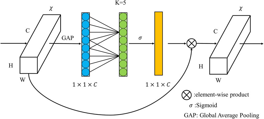
FIGURE 3. Structure of ECA module.

The ECANet generates weights for each channel by a one-dimensional convolution of size $\mathrm{K}$. Where $\mathrm{\omega }$ denotes the output value. Details as shown in Eq. 10.

$\mathrm{\omega }=\mathrm{\sigma }\left(\mathrm{C}1{\mathrm{D}}_{\mathrm{K}}\left(\mathrm{y}\right)\right)(10)$

In the formula, $\mathrm{C}1\mathrm{D}$ denotes a one-dimensional convolution, $\mathrm{y}$ denotes a channel, and $\mathrm{\sigma }$ denotes a Sigmoid activation function; the larger the channel dimension, the larger the range of local cross-channel interactions. The mapping between the channel dimensions $\mathrm{C}$ and $\mathrm{K}$ is as shown in Eq. 11.

$\mathrm{C}=\varnothing \left(\mathrm{K}\right)\approx \exp \left(\mathrm{\gamma }\times \mathrm{K}-\mathrm{b}\right)(11)$

$\mathrm{K}$ is calculated by the Eq. 12.

$\mathrm{K}=\mathrm{\phi }\left(\mathrm{C}\right)={\left|\frac{{\log }_2\left(\mathrm{C}\right)}{\mathrm{\gamma }}+\frac{\mathrm{b}}{\mathrm{\gamma }}\right|}_{\text{odd}}(12)$

In the equation, $\mathrm{C}$ denotes the input feature channel dimension, ${\left|\mathrm{t}\right|}_{\text{odd}}$ denotes the closest odd number to $\mathrm{t}$, the value of $\mathrm{\gamma }$ is set to 2, and the value of $\mathrm{b}$ is set to 1.

2.6 Replacing the Cross Entropy Loss Function with focal loss

Loss refers to the difference between the output value of the model and the true value of that sample, and the loss function describes that difference. For a deep learning model, the neural network weights in the model are trained by loss back propagation. Thus, the loss function plays an important role in the training effectiveness of the model. The paper uses a focal loss function instead of a cross-entropy loss function to cope with the problem of multiple categorizations and the imbalance in the proportion of categorized objects.

Focal Loss is on the basis of binary cross entropy (CE), which is a dynamically scaled cross entropy loss. With a dynamic scaling factor, the weight of easily distinguishable samples during training can be dynamically reduced to quickly focus on those that are difficult to distinguish. The calculations for the following formulas are derived from the article published by Lin et al. (2017) at the ICCV conference in 2017.

The formula for cross-entropy loss is as shown in Eq. 13.

$\text{CE}\left(\mathrm{p},\mathrm{y}\right)=\left\{\begin{array}{c}-\log \left(\mathrm{p}\right)\text{\hspace{1em}if\hspace{0.17em}}\mathrm{y}=1\\ -\log \left(1-\mathrm{p}\right)\text{\hspace{1em}otherwise}\end{array}\right.(13)$

In the above equation, $\mathrm{y}$ takes the values of 1 and −1, representing foreground and background, respectively. The value of $\mathrm{p}$ ranges from 0–1 and is the probability that the model predicts belonging to the foreground. Next define a function with respect to $\mathrm{p}$. Details as shown in Eq. 14.

${\mathrm{p}}_{\mathrm{t}}=\left\{\begin{array}{c}\mathrm{p}\text{\hspace{1em}if\hspace{0.17em}}\mathrm{y}=1\\ 1-\mathrm{p}\text{\hspace{1em}otherwise}\end{array}\right.(14)$

Combining the above equations, Eq. 15 can be obtained.

$\text{CE}\left(\mathrm{p},\mathrm{y}\right)=\text{CE}\left({\mathrm{p}}_{\mathrm{t}}\right)=-\log \left({\mathrm{p}}_{\mathrm{t}}\right)(15)$

Balanced Cross Entropy (BCE) is a common solution to class imbalance. A weight factor $\mathrm{\alpha }\in \left[0,1\right]$ is introduced, which is $\mathrm{\alpha }$ when it is a positive sample and $1-\mathrm{\alpha }$ when it is a negative sample. So, the loss function can also be rewritten as shown in Eq. 16.

$\text{CE}\left({\mathrm{p}}_{\mathrm{t}}\right)=-{\mathrm{\alpha }}_{\mathrm{t}}\log \left({\mathrm{p}}_{\mathrm{t}}\right)(16)$

Although BCE solves the problem of unbalanced positive and negative samples, it does not distinguish between simple or complex samples. When there are more simple negative samples, the entire training process will revolve around the simple negative samples, which in turn will drown out the positive samples and cause large losses. Therefore, a modulation factor is introduced for focusing complex samples. By balancing for positive and negative samples as well as simple and complex samples, the Eq. 17 for the final Focal Loss can be obtained.

$\text{FL}\left({\mathrm{p}}_{\mathrm{t}}\right)=-{\mathrm{\alpha }}_{\mathrm{t}}{\left(1-{\mathrm{p}}_{\mathrm{t}}\right)}^{\mathrm{\gamma }}\log \left({\mathrm{p}}_{\mathrm{t}}\right)(17)$

In the formula, the inhomogeneity of the sample proportions is balanced by the weights ${\mathrm{\alpha }}_{\mathrm{t}}$, which takes values in the range $\left[0,1\right]$. $\mathrm{\gamma }$ is a hyperparameter, and the value of $\mathrm{\gamma }$ is in the range of $\left[0,5\right]$. When the value of $\mathrm{\gamma }$ is 0, the focal loss is the traditional CE loss. ${\mathrm{p}}_{\mathrm{t}}$ is the predicted probability of different categories, the smaller the value of ${\mathrm{p}}_{\mathrm{t}}$ the more difficult it is to categorize, the larger the value of the indicator of ${\left(1-{\mathrm{p}}_{\mathrm{t}}\right)}^{\mathrm{\gamma }}$, the easier it is to categorize. For simple and easy-to-learn samples, the larger the corresponding predictive probability, the smaller the corresponding weight; the smaller the predictive probability, the larger the weight for composite samples.

3 Experiments

3.1 Experimental software and hardware configurations

PyTorch deep learning framework is used in this paper for training and testing of network models. The specific experimental software and hardware configurations are shown in Table 2.

TABLE 2

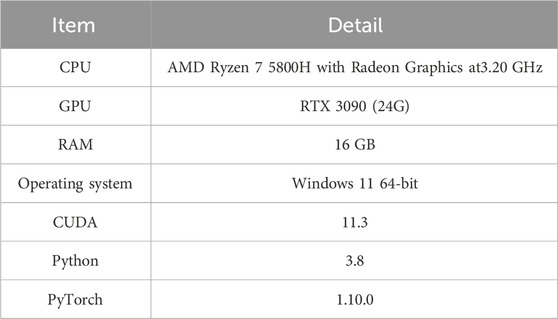
TABLE 2. Experimental hardware and software configuration.

3.2 Experimental datasets

Two main datasets are used for the experiments in this paper. A publicly available dataset WHDLD (Shao et al., 2018) and a home-made dataset FRSID. Since the data content of the dataset WHDLD as well as other publicly available datasets are mostly remote sensing images of an area as a whole, there is no careful differentiation between research objects or influencing factors. Therefore, a new dataset FRSID is created by ourselves. It containing land cover remote sensing images classified according to several factors affecting segmentation accuracy such as main categories and percentages, shadow percentage, number of categories, etc. The dataset is used to test the influences of different factors on the segmentation accuracy, so as to verify the robustness of the DeepGDLE network proposed in this paper.

3.2.1 WHDLD

WHDLD is the WuHan Dense Labeled Dataset, is a publicly available dataset. The dataset includes 4,940 images taken by Gaofen-1 and Ziyuan-3 satellite sensors in Wuhan, with a standard resolution of 256*256 pixels RGB images and a spatial resolution of 2 m.

The image annotation categories in the dataset are organized into six categories: bare land, building, sidewalk, water body, vegetation, and road.

3.2.2 FRSID

FRSID is the Fuyang Remote Sensing Image Dataset, is the new dataset created in this paper. The content of the dataset is the remote sensing images of the Fuyang District area of Hangzhou City, Zhejiang Province in 2021. The study area is located in the northwestern part of Zhejiang Province, between 119°25′ and 120°19.5′E longitude and 29°44′ and 30°11′N latitude. It has a humid subtropical monsoon climate and the topography is dominated by hills and mountains.

This dataset contains 900 original remote sensing images around the main urban area of Fuyang, and the resolution is standardized as 600*600 pixels RGB images. All contained categories in the dataset were labeled and stored through the graphical interface labeling software LabelMe (Russell et al., 2008), JSON files were generated. The data labels were converted into binarized png images using the JSON to dataset command. The dataset is stored in the PASCAL VOC (Vicente et al., 2014) data format. Using the data enhancement tool, the dataset is augmented with a combination of operations including but not limited to random rotation, mirroring, etc. to expand the dataset and finally increase the number of datasets to 4500 RGB images to improve the generalization ability. The spatial resolution is 2 m.

The image annotation categories in the dataset are categorized into eight categories: cropland, vegetation, building, water body, general road, parking lot, main road, and playground.

3.3 Dataset classification

In order to test the impact of different factors present in the dataset on the semantic segmentation performance of rural land cover remote sensing images to validate the robustness of the DeepGDLE model proposed in this paper, the FRSID dataset is classified in this paper according to the following three factors that affect the segmentation accuracy: 1) main category and its percentage; 2) shadow percentage; 3) category count. This results in three sub-datasets: Dataset with different Main Categories and Percentages (DataMCP), Dataset with different Shadow Percentages (DataSP), and Dataset with different Categories Counts (DataCC).

3.3.1 Dataset with different main categories and percentages (DataMCP)

This dataset is primarily divided on the basis of the main category of the image and its percentage. Firstly, the data images were divided according to the different main categories in the data images, which were building cover, vegetation cover, cropland cover and water body cover, four types in total. These four main categories were identified as the main body in the respective data image as they occupied more than 50% of the whole image and the rest of the categories were less than 50%. The data images were then further subdivided according to the percentage ranges of 50%–75% and 75%–100% to obtain eight sub-datasets. The samples of the DataMCP dataset are shown in Supplementary Figure S7, and the details are shown in Table 3.

TABLE 3

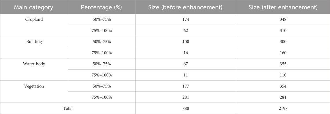
TABLE 3. Size of DataMCP dataset.

3.3.2 Dataset with different shadow percentages (DataSP)

This dataset is mainly divided on the basis of the shadow percentage in the data images. The shadow percentage is one of the factors affecting the segmentation accuracy, but the percentage of shadows in most of the data images is relatively small, and most of the shadows are below 15%. In order to better test the influence of shadow percentage on segmentation accuracy, the data images with shadows are divided according to four percentage intervals: 0%–5%, 5%–10%, 10%–15%, and 15%–100%, and four sub-datasets are obtained. The data samples in the DataSP dataset are shown below in Supplementary Figure S8, and the contents of the dataset are shown in Table 4.

TABLE 4

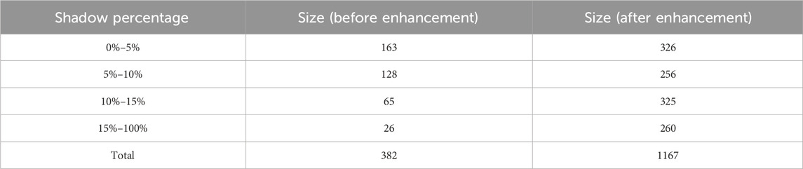
TABLE 4. Size of DataSP dataset.

3.3.3 Dataset with different Categories Counts (DataCC)

This dataset is primarily divided on the basis of the category count in the image. Different categories represent different levels of complexity in the image. A total of eight different categories exist in the dataset and four sub-datasets are obtained by dividing them according to the number of categories {1, 2}, {3, 4}, {5, 6}, {7, 8}. Samples of the DataCC dataset is shown in Supplementary Figure S9. The contents of the dataset are shown in Table 5.

TABLE 5

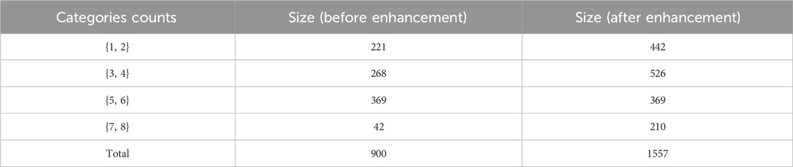
TABLE 5. Size of DataCC dataset.

3.4 Evaluation indicators

In this experimental study, the following metrics were used in order to evaluate the segmentation performance of the high-resolution remote sensing image dataset, mean Intersection over Union (mIoU), mean Pixel Accuracy (mPA) and mean Recall (mRecall). This metric is a common evaluation metric in the field of computer vision to measure the performance of a model in tasks such as semantic segmentation and target detection.

3.4.1 mean Intersection over Union (mIoU)

The mIoU is the most commonly used evaluation metric in experimental studies of semantic segmentation. mIoU first calculates the ratio of the intersection and concatenation of the two sets of true and predicted values on each category, and then averages the intersection and concatenation ratios over all categories. The formula is as shown in Eq. 18.

$\text{mIoU}=\frac{1}{\mathrm{n}}{\displaystyle \sum _{\mathrm{i}=0}^{\mathrm{n}}}\frac{{\mathrm{p}}_{\text{ii}}}{{\displaystyle \sum _{\mathrm{j}=0}^{\mathrm{n}}}{\mathrm{p}}_{\text{ij}}+{\displaystyle \sum _{\mathrm{j}=0}^{\mathrm{n}}}{\mathrm{p}}_{\text{ji}}-{\mathrm{p}}_{\text{ii}}}(18)$

3.4.2 mean Pixel Accuracy (mPA)

The mPA is the average of the ratio of correctly predicted pixel points to total pixel points for all categories. The formula is as shown in Eq. 19.

$\text{mPA}=\frac{1}{\mathrm{n}}{\displaystyle \sum _{\mathrm{i}=0}^{\mathrm{n}}}\frac{{\mathrm{p}}_{\text{ii}}}{{\displaystyle \sum _{\mathrm{i}=0}^{\mathrm{n}}}{\displaystyle \sum _{\mathrm{j}=0}^{\mathrm{n}}}{\mathrm{p}}_{\text{ij}}}(19)$

3.4.3 mean Recall (mRecall)

mRecall is the average of the sum of the ratios of the number of pixel points correctly categorized in each category to the number of pixel points predicted to be in that category. The formula is as shown in Eq. 20.

$\text{mRecall}=\frac{1}{\mathrm{n}}{\displaystyle \sum _{\mathrm{i}=0}^{\mathrm{n}}}\frac{{\mathrm{p}}_{\text{ii}}}{{\mathrm{p}}_{\text{ii}}+{\displaystyle \sum _{\mathrm{i}=0}^{\mathrm{n}}}{\mathrm{p}}_{\text{ji}}}(20)$

In this formula, $\mathrm{n}$ is the total category, ${\mathrm{p}}_{\text{ij}}$ represents the number of pixels that would have belonged to category $\mathrm{i}$ but were predicted to be in category $\mathrm{j}$, ${\mathrm{p}}_{\text{ij}}$ represents the number of pixels that would have belonged to category $\mathrm{j}$ but were predicted to be in category $\mathrm{i}$, ${\mathrm{p}}_{\text{ii}}$ represents the number of correct predictions, and ${\mathrm{p}}_{\text{ij}}$ and ${\mathrm{p}}_{\text{ji}}$ are false positive and false negative, respectively.

3.5 Experimental schemes

3.5.1 Determination of training parameters

Each dataset for the experiments was divided into a training set with 80% data, a validation set with 10% data, and a test set with 10% data. All models were implemented using PyTorch. The accuracies of the model DeepGDLE under different learning rates and batch sizes using publicly available remote sensing image datasets were tested, and the final selection of training parameters is shown in Table 6. In order to improve the accuracy of model segmentation, GhostNet pre-training weights are loaded before model training. The focal loss function, Focal Loss, is used to reduce the impact of the large difference in the proportion of feature categories in the dataset on the accuracy of model feature classification.

TABLE 6

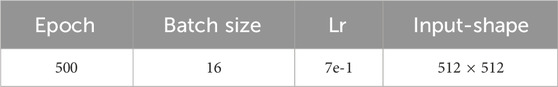
TABLE 6. Optimal training parameters.

3.5.2 Experimental scheme for dilation rate selection in ASPP modules

In order to study the performance of segmentation under different dilation rate settings for parallel convolution in the ASPP module, four cases with different dilation rates are selected to test the relationship of the dilation rate on the network. Four dilation rates, 1/2/5/9, 1/5/9/17, 1/6/12/18, and 1/2/7/15, were selected. The mPA, mRecall, and mIoU were selected as metrics to evaluate the comparison.

3.5.3 Experimental scheme for performance comparison

In order to test the performance of DeepGDLE, the model proposed in this paper, in remote sensing image segmentation tasks, comparative experiments are conducted with DeepGDLE and traditional semantic segmentation methods such as SegNet, PSPNet, UNet, and DeeplabV3+. The mIoU, mPA, and mRecall are selected as metrics to test the segmentation performance of this paper’s method. Training time, single-image prediction time and number of parameters are selected as metrics to test the segmentation efficiency of the method in this paper.

3.5.4 Experimental scheme for robustness analysis

In order to test the generalization ability of DeepGDLE proposed in this paper and the robustness of the method, experiments are conducted on the DataMCP dataset containing different main categories and their percentages, the DataSP dataset containing different shadow percentages, and the DataCC dataset containing different Categories counts, which are classified according to different factors. The mIoU, mPA, and mRecall are selected as metrics to test the robustness of the method in this paper.

3.5.5 Scheme of ablation experiments

In order to verify the contribution to segmentation performance of the DeepGDLE aspects proposed in this paper, four different improvement modules are used to perform segmentation performance ablation experiments and segmentation efficiency ablation experiments on two differently categorized total datasets. Because the introduction of Focal Loss is an optimization of the loss function of the model calculation results, it has little effect on the model structure. Therefore, this experiment combines Focal Loss with the traditional DeeplabV3+ model.

In order to verify the segmentation performance of DeepGDLE, GhostNet is considered to be able to acquire more image information by using linear operations to generate more feature mappings. The ECANet attention mechanism learns the channel attention of each convolutional block, uses one-dimensional convolution to avoid dimensionality reduction operations, efficiently realizes cross-channel interactions. This provides appropriate weights for the channels, and brings significant performance gains to the architecture of the network. And the ECANet attention mechanism was added at two different sites. Therefore, a total of seven modelling experiments are conducted for comparison, as described in detail as follows.

(1) DeepL: In the original DeeplabV3+ model, the Focal Loss function is introduced.

(2) DeepGL: On the basis of DeepL, the feature extraction network was replaced with the GhostNet network.

(3) DeepLE1: On the basis of DeepL, only the ECANet Attention module is added after the Feature Extraction module.

(4) DeepLE2: On the basis of DeepL, add the ECANet Attention module to DeepL after the ASPP module only.

(5) DeepLE: On the basis of DeepL, the ECANet attention module is added after the feature extraction module and ASPP module at the same time, i.e., the scheme proposed in this paper.

(6) DeepGLE: On the basis of DeepLE, the feature extraction network is replaced with a GhostNet network.

(7) DeepGDLE: The model proposed in this paper.

In order to verify the segmentation efficiency of DeepGDLE, considering that the GhostNet network has a shallower number of layers and fewer parameters, the complexity of the model is lower, and the network is faster in both training and convergence. Depthwise separable convolution divides a standard convolution into two layers, one for filtering and one for combining. The amount of computation and the number of parameters of the model are drastically reduced while maintaining the accuracy upfront. Therefore, a total of five modelling experiments are conducted for comparison, as described in detail as follows.

(1) DeepL: In the original DeeplabV3+ model, the Focal Loss function is introduced.

(2) DeepGL: On the basis of DeepL, the feature extraction network was replaced with the GhostNet network.

(3) DeepDL: On the basis of DeepL, the ordinary convolution in the ASPP module was replaced with depthwise separable convolution.

(4) DeepGDL: On the basis of DeepDL, the feature extraction network is replaced with a GhostNet network.

(5) DeepGDLE: The model proposed in this paper.

4 Results and analysis

4.1 Dilation rate selection in ASPP module

In this section, four cases with different dilation rates are selected to test the relationship between the effects of dilation rates on the network. Four dilation rates of 1/2/5/9, 1/5/9/17, 1/6/12/18, and 1/2/7/15 were considered. The evaluation metrics are mPA, mRecall, and mIoU. The specific results of the experiment are shown in Table 7.

TABLE 7

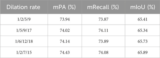
TABLE 7. Dilation rate comparison experiment.

According to the indicators of performance using different dilation rates in Table 7, the model’s mPA is 74.43%, mRecall is 74.08%, and mIoU is 65.89% when the dilation rate is 1/2/7/15, which is overall better than the other three dilation rates. Hence the final dilation rate is determined as 1/2/7/15.

4.2 Segmentation results

In order to validate the segmentation performance of the model DeepGDLE proposed in this paper, the method is compared with other semantic segmentation models SegNet, PSPNet, UNet, DeepLabV3+(Xception), DeepLabV3+(MobileNetV2) models. The segmentation comparison results for some of the images are shown in Figures 4, 5.

FIGURE 4

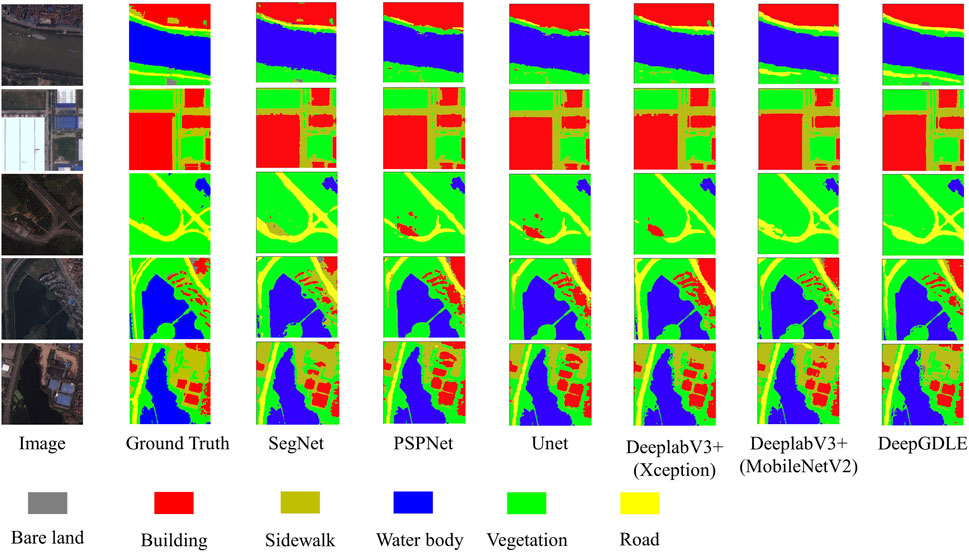
FIGURE 4. Results of different methods by using WHDLD dataset.

FIGURE 5

FIGURE 5. Results of different methods by using FRSID dataset.

From Figures 4, 5, it can be seen that the DeepGDLE segmentation of this paper’s method outperforms the five semantic segmentation models of SegNet, PSPNet, UNet, DeeplabV3+(Xception), and DeeplabV3+(MobileNetV2). DeepGDLE is better for segmentation of edges between categories and has fewer segmentation errors and segmentation misses, which proves that the method DeepGDLE in this paper has better segmentation performance.

4.2.1 Segmentation performance

Using mIoU, mPA, and mRecall as metrics, the results for the WHDLD dataset are shown in Table 8 and the FRSID dataset is shown in Table 9.

TABLE 8

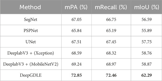
TABLE 8. Segmentation performance results of different methods for WHDLD dataset.

TABLE 9

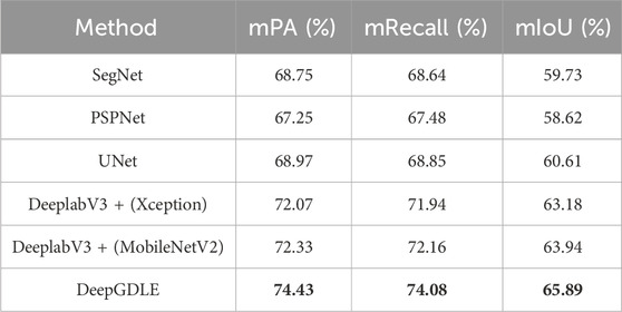
TABLE 9. Segmentation performance results of different methods for FRSID dataset.

From Tables 8, 9, it can be seen that the DeepGDLE method proposed in this paper outperforms other networks. Regarding the segmentation performance, the mPA of DeepGDLE in the WHDLD dataset results is 72.85%, which is improved by 8.59%, 10.65%, 7.90%, 6.21%, and 5.21% over that of SegNet, PSPNet, UNet, DeeplabV3+ (Xception), and DeeplabV3+ (MobileNetV2), respectively. The mRecall of DeepGDLE is 72.46%, which is improved by 8.55%, 11.15%, 7.43%, 6.06%, and 5.06% over that of SegNet, PSPNet, UNet, DeepLabV3+ (Xception), and DeeplabV3+ (MobileNetV2), respectively. The mIoU of DeepGDLE is 62.29%, which is improved by 10.07%, 11.45%, 7.86%, 6.00%, and 4.04% over that of SegNet, PSPNet, UNet, DeepLabV3+ (Xception), and DeeplabV3+ (MobileNetV2), respectively. The mPA of DeepGDLE in the FRSID dataset results is 74.43%, which is improved by 8.26%, 10.68%, 7.92%, 3.27%, and 2.90% over that of SegNet, PSPNet, UNet, DeepLabV3+ (Xception), and DeeplabV3+ (MobileNetV2), respectively. The mRecall of DeepGDLE is 74.08%, which is improved by 7.93%, 9.78%, 7.60%, 2.97%, and 2.66% over that of SegNet, PSPNet, UNet, DeepLabV3+ (Xception), and DeeplabV3+ (MobileNetV2), respectively. The mIoU of DeepGDLE is 65.89%, which is improved by 10.31%, 12.40%, 8.71%, 4.29%, and 3.05% over that of SegNet, PSPNet, UNet, DeepLabV3+ (Xception), and DeeplabV3+ (MobileNetV2), respectively.

The experimental results show that DeepGDLE outperforms the other five comparison models on both datasets. The use of GhostNet as a feature extraction network in DeepGDLE, as well as the improvement of incorporating ECANet’s attention mechanism, improves the feature extraction capability and segmentation accuracy of various types of images in the test set of remote sensing images, which further proves the performance of the DeepGDLE method.

4.2.2 Segmentation efficiency

Using training time, single image prediction time, and number of parameters as metrics for comparison, the results for the WHDLD dataset are shown in Table 10 and the results for the FRSID dataset are shown in Table 11.

TABLE 10

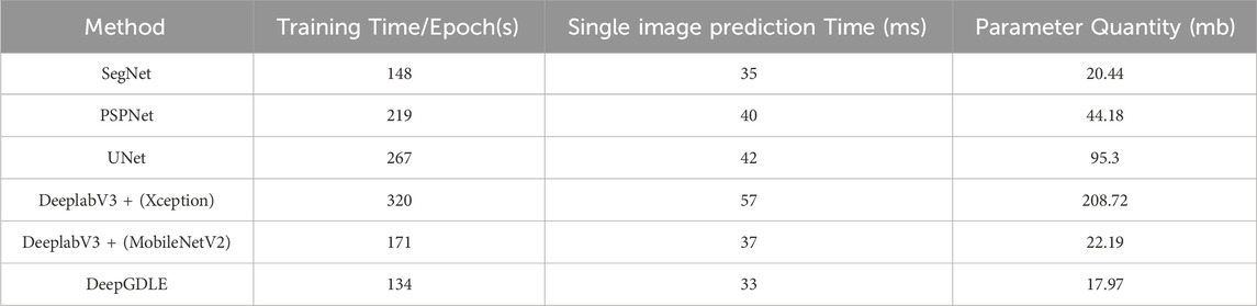
TABLE 10. Segmentation efficiency results of different methods for WHDLD dataset.

TABLE 11

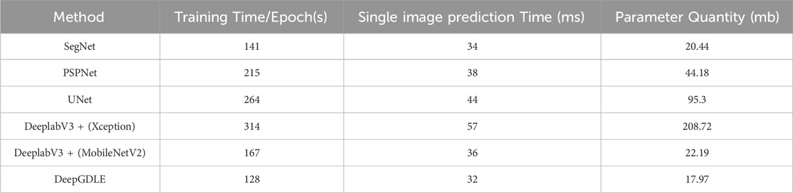
TABLE 11. Segmentation efficiency results of different methods for FRSID dataset.

According to the data analysis of experimental results in Tables 10, 11. In terms of segmentation efficiency, the training time per epoch of DeepGDLE in the WHDLD dataset is 134 s, the efficiency is improved by 9.46%, 38.81%, 49.81%, 58.13%, and 21.64% over that of PSPNet, UNet, DeepLabV3+ (Xception), and DeeplabV3+ (MobileNetV2), respectively. The prediction time single image of DeepGDLE is 34 ms. The efficiency is improved by 2.86%, 15.00%, 19.05%, 40.35%, and 8.11% over that of PSPNet, UNet, DeeplabV3+(Xception), and DeeplabV3+(MobileNetV2), respectively. The training time per epoch of DeepGDLE in the FRSID dataset is 128 s. The efficiency is improved by 9.22%, 40.47%, 51.52%, 59.24%, and 23.35% over that of PSPNet, UNet, DeepLabV3+ (Xception), and DeeplabV3+ (MobileNetV2), respectively. The prediction time single image of DeepGDLE is 34 ms. The efficiency is improved by 5.88%, 15.79%, 27.27%, 43.86%, and 25.00% over that of PSPNet, UNet, DeeplabV3+(Xception), and DeeplabV3+(MobileNetV2), respectively. Regarding the number of parameters, DeepGDLE is 17.97 mb, which is 2.47 mb, 26.21 mb, 77.33 mb, 190.75 mb, and 4.22 mb lower than the number of parameters of PSPNet, UNet, DeeplabV3+(Xception), and DeeplabV3+(MobileNetV2), respectively.

Overall, since the model DeepGDLE uses GhostNet to replace the Xception feature extraction network for extracting information and replaces the normal convolution in the ASPP module with a depthwise separable convolution, it reduces the overall number of parameters of the model compared to other network models in the experiments, making the model lighter, reducing the training and prediction time, and improving the segmentation efficiency.

4.3 Robustness analysis

In order to test the robustness of the method, experiments were done to compare the segmentation effects on the DataMCP dataset containing different main categories and their percentages, the DataSP dataset containing different shadow percentages, and the DataCC dataset containing different Categories counts, using the models trained from the FRSID dataset. Using mPA, mRecall, and mIoU as evaluation metrics.

4.3.1 Influence of main category and percentage

Segmentation experiments are performed on the DataMCP dataset. Using mPA, mRecall, and mIoU as evaluation metrics. The comparison results for DataMCP dataset are shown in Table 12.

TABLE 12

TABLE 12. Comparison of segmentation performance for DataMCP.

As can be seen in Table 12, the segmentation exhibited in the dataset dominated by cropland and water cover is more effective. The mIoU can reach up to 72.49% and 80.14%, mPA can reach up to 81.28% and 89.34%, and mRecall can reach up to 80.89% and 89.04%, respectively. The overall segmentation is better than in cases where complex buildings or vegetation cover are the mainstay. The mIoU was 56.47% and 61.64%, the mPA was 66.39% and 70.89%, and the mRecall was 66.14% and 70.48% for the case where complex buildings and vegetation cover were the mainstay, respectively.

In the case of four different main categories, the dataset with cropland and water body cover as the main categories has clear boundaries between categories in the image, which interferes less with segmentation, and the shape of the labels is more regularized and the segmentation is more effective, compared to the dataset with complex buildings and vegetation cover as the main category. Also, when the categories are the same, the larger the percentage, the better the segmentation.

4.3.2 Influence of shadow percentage

Segmentation experiments are performed on the DataSP dataset. Using mPA, mRecall, and mIoU as evaluation metrics. The comparison results for DataSP dataset are shown in Table 13.

TABLE 13

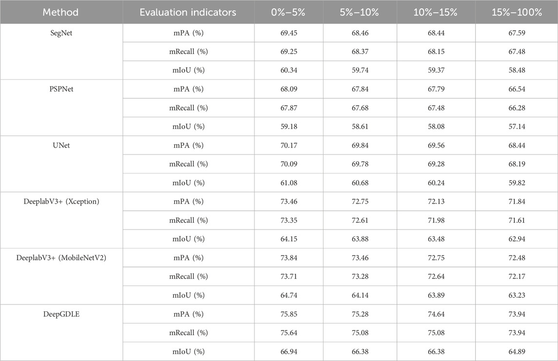
TABLE 13. Comparison of segmentation performance for DataSP.

From Table 13, it can be seen that in the presence of shadows, different shadow percentages lead to a decrease in segmentation. The best performing DeepGDLE model mPA is 75.85%, mRecall is 75.64%, and mIoU is 66.94% when the shadow percentage is in the 0%–5% range. The best performing DeepGDLE model mPA is 75.28%, mRecall is 75.08%, and mIoU is 66.38% when the shadow percentage is in the 5%–10% range. The best performing DeepGDLE model mPA is 72.48%, mRecall is 72.17%, and mIoU is 64.89% when the shadow percentage is in the 10%–15% range.

The larger the percentage of shadows in the dataset image, the worse the overall segmentation will be. Shadows can lead to wrong scores as well as missed scores because the shading interferes with the overall segmentation. Shadows themselves are not part of the categories delineated in the dataset, and the greater the percentage of shadows, the greater the impact on category segmentation. But while shading is also a factor that affects segmentation accuracy, the effect is not as large as that of the category and its percentage and category counts.

4.3.3 Influence of category count

Segmentation experiments are performed on the DataCC dataset. Using mPA, mRecall, and mIoU as evaluation metrics. The comparison results for DataCC dataset are shown in Table 14.

TABLE 14

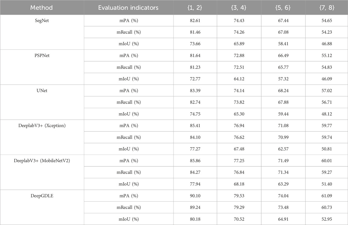
TABLE 14. Comparison of segmentation performance for DataCC.

From Table 14, it can be seen that the more category counts in the image, the more the segmentation accuracy of the model decreases to some extent. The best performing DeepGDLE model with category counts {1, 2} was 90.10% for mPA, 89.24% for mRecall and 80.18 for mIoU. The best performing DeepGDLE model with category counts {3, 4} was 79.53% for mPA, 79.29% for mRecall and 70.52% for mIoU. The best performing DeepGDLE model with category counts {5, 6} was 74.04% for mPA, 73.48% for mRecall and 64.91% for mIoU. The best performing DeepGDLE model with category {7, 8} was 61.09% for mPA, 60.73% for mRecall and 52.95% for mIoU.

From the data in the table, when the category counts in the dataset is small and there are only one or two category counts, the accuracy of the model segmentation is very good and the mIoU can reach more than 80%. However, as the category counts in the image increases, the segmentation performance of the overall model decreases. The model’s segmentation accuracy performance is worst when the category counts in the image reaches a maximum of eight. Different category counts represent different complexity of information in the image, and an increase in the category counts represents an increase in the amount of information in the image. Therefore, the complexity of the data image content is also one of the factors affecting the model segmentation accuracy.

4.4 Results of ablation experiments

4.4.1 Split performance ablation experiment results

The experiments in this section were conducted according to the ablation experimental program of 3.5.5. The evaluation metrics are mPA, mRecall, and mIoU. The specific results of the experiment are shown in Figures 6, 7, Tables 15, 16.

FIGURE 6

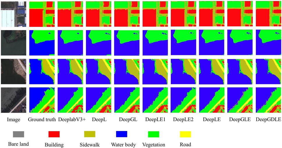
FIGURE 6. Segmentation performance ablation experiment results by using WHDLD dataset.

FIGURE 7

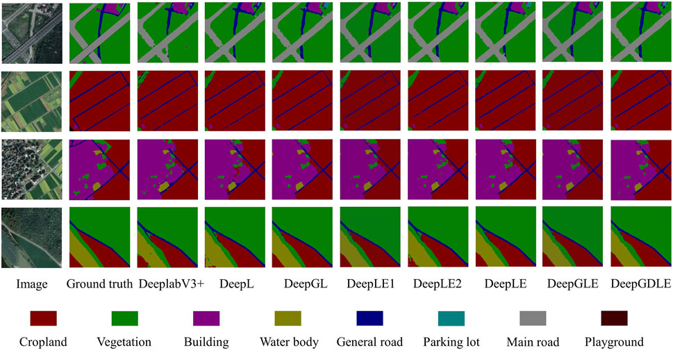
FIGURE 7. Segmentation performance ablation experiment results by using FRSID dataset.

TABLE 15

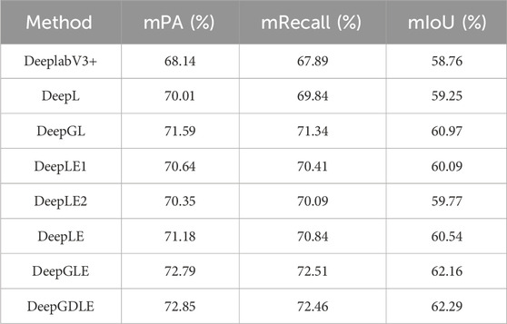
TABLE 15. WHDLD dataset segmentation performance results.

TABLE 16

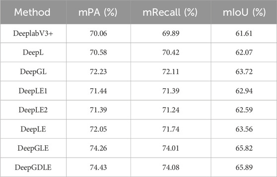
TABLE 16. FRSID dataset segmentation performance results.

According to the results of the model doing segmentation performance ablation experiments on two different datasets, it can be seen that comparing DeeplabV3+ with DeepL, there is an improvement in the mPA, mRecall, and mIoU. It is shown that the segmentation accuracy of the model is improved when the Focal Loss is introduced in the model.

Comparing the DeepLE1, DeepLE2, and DeepLE models, the metrics in mPA, mRecall, and mIoU are better than DeepL. However, relatively speaking, model DeepLE1 improves the segmentation performance better than the case of model DeepLE2, so this improvement after ECANet’s attention mechanism was added to the feature extraction module is the main reason why the attention mechanism improves the segmentation performance.

Comparing DeepL and DeepGL, as well as DeepLE and DeepGLE, the mPA, mRecall, and mIoU are improved. It is shown that replacing the feature extraction network with GhostNet improves the segmentation accuracy of the model to some extent. At the same time this improvement improves the performance metrics to a better extent than the inclusion of the ECANet attention mechanism. Therefore, replacing the feature extraction network with GhostNet is the main reason for improving the segmentation performance in the overall model.

4.4.2 Segmentation efficiency ablation experiment results

The experiments in this section were performed according to the ablation experimental program of 3.5.5. The evaluation metrics are training time, single image prediction time, and parameter quantity.

The specific results of the experiment are shown in Tables 17, 18.

TABLE 17

TABLE 17. Segmentation efficiency results for WHDLD dataset.

TABLE 18

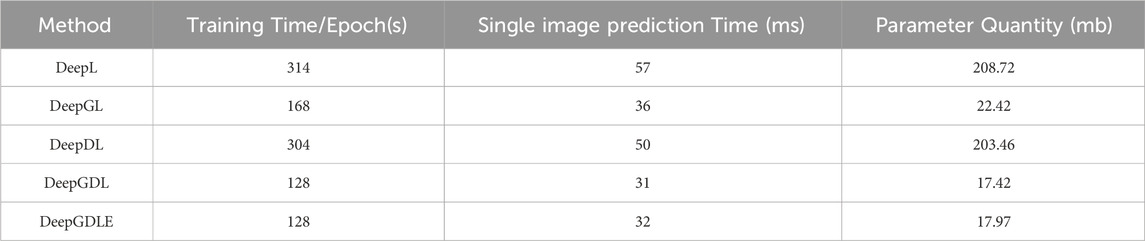
TABLE 18. Segmentation efficiency results for FRSID dataset.

According to the results of the model doing segmentation efficiency ablation experiments on two different datasets, it can be seen that comparing DeepL and DeepGL, there is an improvement for DeepGDLE in the three values of training time, single image prediction time, and parameter quantity. It is illustrated that the use of a lightweight network, GhostNet, reduces the parameters of the entire model and therefore reduces the training time of the model as well as improves the speed of model prediction.

Compared to DeepL and DeepDL, DeepGDLE improves on three metrics: training time, single image prediction time, and parameter quantity. It is illustrated that replacing the ordinary convolution in the ASPP module with depthwise separable convolution also reduces the parameters of the model, which further reduces the training time and improves the prediction speed.

Comparing DeepL, DeepGL, DeepDL, and DeepGDL, although both improvements for DeepGDLE are able to reduce the parameters of the model, shorten the model training time, and increase the speed of the model prediction. But the improvement of using a lightweight network, GhostNet, is the main reason for the increased segmentation efficiency.

5 Conclusion

A lightweight land cover classification method with an attention mechanism on the basis of semantic segmentation of remote sensing images, DeepGDLE, was proposed in this paper. The DeepGDLE method is on the basis of the traditional DeeplabV3+ network, and the GhostNet network is used as the backbone extraction feature network, which significantly reduces the number of parameters in the feature extraction network and lightens the model. A depthwise separable convolution is used to replace the normal convolution in the ASPP module, effectively reducing the overall number of parameters in the model. The dilation rate of parallel convolution in the ASPP module is optimized to avoid the “grid effect”. The ECANet attention mechanism is added after the feature extraction module and the ASPP module, which utilizes an efficient channel attention mechanism to obtain more data information features, improve the overall segmentation ability of the model. It can avoid dimensionality reduction and reduce the phenomenon of omission and misjudgment at the same time. And for the reason that the proportions of different categories in the dataset are different, the focal loss function, Focal Loss, is used to balance the samples by assigning different proportional weights to different categories.

The proposed model, DeepGDLE, can effectively segment remote sensing images. The mIoU of DeepGDLE on two remote sensing image datasets reaches 62.29% and 65.89%, and the $\text{mPA}$ reaches 72.85% and 74.43%, respectively. More efficient and accurate segmentation of high-resolution remote sensing images is realized. A dataset FRSID of remote sensing images is established, which has more consideration about the influencing factors of semantic segmentation of remote sensing imagery. The experiments of method DeepGDLE on the WHDLD dataset, FRSID dataset fully confirm that the method outperforms the benchmark method. The robustness of the method DeepGDLE is successfully verified through comparison experiments with five different semantic segmentation methods, namely, SegNet, PSPNet, UNet, DeeplabV3+(Xception), and DeeplabV3+(MobileNetV2), on the DataMCP dataset, which contains different Main Categories and Percentages, the DataSP dataset, which contains different Shadow Percentages, and the DataCC dataset, which contains different Categories. It is also demonstrated that DeepGDLE outperforms other methods for different factors.

The factors affecting the segmentation performance of the model are analyzed through robustness experiments performed on datasets classified under three different scenarios. Among them, different main categories and percentages have some influence on the segmentation performance of the model, and the segmentation in the dataset with cropland and water body cover as the main categories is better, and the overall segmentation effect is better than that of the case with building cover or vegetation cover as the main categories. The more distinct the edges between categories, the more detailed the segmentation. Also, the larger the category share, the better the segmentation. Moreover, the different shadow percentages are one of the factors affecting the model segmentation performance. In the presence of shadows, different shadow percentages result in a certain reduction in segmentation. The larger the shadow percentages, the worse the overall segmentation. Finally, the different category counts in the image is also a factor that affects the segmentation performance, the more the category counts, the more complex the information in the image, the worse the segmentation effect of the overall model.

The future work of this study focuses on the following aspects. Firstly, for the categories with low segmentation accuracy, study the reasons and make improvements accordingly, so as to improve the segmentation accuracy of the overall model. Secondly, there are uncertain factors in the segmentation such as lack of clarity in the segmentation between categories and categories, and the presence of a large area of shadows interferes with the accuracy of the segmentation model, so explore how to reduce the interference of these factors. Thirdly, produce more remote sensing images and more kinds of land cover information data for experiments, and try to use algorithm-assisted methods of semi-automatic or fully-automatic data annotation, so as to expand the dataset and obtain more usable data.

Data availability statement

The original contributions presented in the study are included in the article/Supplementary Material, further inquiries can be directed to the corresponding authors.

Author contributions

GW: Conceptualization, Investigation, Methodology, Resources, Writing–review and editing. JC: Conceptualization, Data curation, Formal Analysis, Investigation, Methodology, Software, Validation, Writing–original draft. LM: Funding acquisition, Investigation, Methodology, Resources, Writing–review and editing. PW: Formal Analysis, Funding acquisition, Investigation, Methodology, Writing–review and editing. XY: Formal Analysis, Investigation, Methodology, Writing–review and editing.

Funding

The author(s) declare financial support was received for the research, authorship, and/or publication of this article. This study was supported by the Key Research and Development Program of Zhejiang Province (Grant number: 2021C02005) and the Natural Science Foundation of China (Grant number: U1809208).

Conflict of interest

The authors declare that the research was conducted in the absence of any commercial or financial relationships that could be construed as a potential conflict of interest.

Publisher’s note

All claims expressed in this article are solely those of the authors and do not necessarily represent those of their affiliated organizations, or those of the publisher, the editors and the reviewers. Any product that may be evaluated in this article, or claim that may be made by its manufacturer, is not guaranteed or endorsed by the publisher.

Supplementary material

The Supplementary Material for this article can be found online at: https://www.frontiersin.org/articles/10.3389/fenvs.2024.1329517/full#supplementary-material

Supplementary Figure S1 | G-bneck module.

Supplementary Figure S2 | Schematic of the standard convolution operation.

Supplementary Figure S3 | Schematic of deep convolution operation.

Supplementary Figure S4 | Schematic of point-by-point convolution operation.

Supplementary Figure S5 | Schematic representation of the dilation rate r = [1, 2, 5].

Supplementary Figure S6 | Schematic representation of the dilation rate r = [1, 2, 9].

Supplementary Figure S7 | Images from DataMCP dataset and their labels. (A) Main category cropland 50%–75%. (B) Main category cropland 75%–100%. (C) Main category building 50%–75%. (D) Main category building 75%–100%. (E) Main category water body 50%–75%. (F) Main category water body 75%–100%. (G) Main category vegetation 50%–75%. (H) Main category vegetation 75%–100%.

Supplementary Figure S8 | DataSP dataset images and their labels. (A) Shadow percentage 0%–5%. (B) Shadow percentage 5%–10%. (C) Shadow percentage 10%–15%. (D) Shadow percentage 15%–100%.

Supplementary Figure S9 | Data CC dataset images and their labels. (A) Categories counts (1, 2). (B) Categories counts (3, 4). (C) Categories counts (5, 6). (D) Categories counts (7, 8).

References

Cao, X., Li, T., Li, H., Xia, S., Ren, F., Sun, Y., et al. (2019). A robust parameter-free thresholding method for image segmentation. IEEE Access 7, 3448–3458. doi:10.1109/ACCESS.2018.2889013

PubMed Abstract | CrossRef Full Text | Google Scholar

Chen, L. C., Papandreou, G., Kokkinos, I., Murphy, K., and Yuille, A. L. (2014). DeepLab: semantic image segmentation with deep convolutional nets, atrous convolution, and fully connected CRFs. IEEE Trans. Pattern Anal. Mach. Intell. 40, 834–848. doi:10.1109/TPAMI.2017.2699184

PubMed Abstract | CrossRef Full Text | Google Scholar

Chen, L.-C., Papandreou, G., Kokkinos, I., Murphy, K., and Yuille, A. L. (2018a). DeepLab: semantic image segmentation with deep convolutional nets, atrous convolution, and fully connected CRFs. IEEE Trans. Pattern Anal. Mach. Intell. 40, 834–848. doi:10.1109/TPAMI.2017.2699184

PubMed Abstract | CrossRef Full Text | Google Scholar

Chen, L.-C., Papandreou, G., Schroff, F., and Adam, H. (2017). Rethinking atrous convolution for semantic image segmentation. Comput. Vis. Pattern Recognit. doi:10.48550/arXiv.1706.0558

CrossRef Full Text | Google Scholar

Chen, L.-C., Zhu, Y., Papandreou, G., Schroff, F., and Adam, H. (2018b). Encoder-decoder with atrous separable convolution for semantic image segmentation. Proc. Eur. Conf. Comput. Vis. (ECCV) 34, 137–143. doi:10.48550/arXiv.1802.02611

CrossRef Full Text | Google Scholar

Chollet, F. (2017). Xception: deep learning with depthwise separable convolutions. Proc. IEEE Conf. Comput. Vis. pattern Recognit. 7, 560–566. doi:10.4271/2014-01-0975

CrossRef Full Text | Google Scholar

Du, S., Du, S., Liu, B., and Zhang, X. (2021). Incorporating DeepLabv3+ and object-based image analysis for semantic segmentation of very high-resolution remote sensing images. Int. J. Digit. Earth 14, 357–378. doi:10.1080/17538947.2020.1831087

CrossRef Full Text | Google Scholar

Fu, G., Liu, C., Zhou, R., Sun, T., and Zhang, Q. (2017). Classification for high resolution remote sensing imagery using a fully convolutional network. Remote Sens. (Basel) 9, 498. doi:10.3390/rs9050498

CrossRef Full Text | Google Scholar

Glorot, X., Bordes, A., and Bengio, Y. (2011). “Deep sparse rectifier neural networks,” in Proceedings of the fourteenth international Conference on artificial Intelligence and statistics proceedings of machine learning research. Editors G. Gordon, D. Dunson, and M. Dudík (Fort Lauderdale, FL, USA: PMLR), 315–323. Available at: https://proceedings.mlr.press/v15/glorot11a.html.

Google Scholar

Guo, Y., Chen, Y., Tan, M., Jia, K., Chen, J., and Wang, J. (2018). Content-aware convolutional neural networks. Proc. IEEE Conf. Comput. Vis. pattern Recognit. 143, 657–668. doi:10.1016/j.neunet.2021.06.030

CrossRef Full Text | Google Scholar

Han, K., Wang, Y., Tian, Q., Guo, J., Xu, C., and Xu, C. (2020). GhostNet: more features from cheap operations. Proc. IEEE/CVF Conf. Comput. Comput. Vis. Pattern Recognit., 1577–1586. doi:10.1109/CVPR42600.2020.00165

CrossRef Full Text | Google Scholar

Hou, Y., Liu, Z., Zhang, T., and Li, Y. (2021). C-UNet: complement UNet for remote sensing road extraction. Sensors 21, 2153. doi:10.3390/s21062153

PubMed Abstract | CrossRef Full Text | Google Scholar

Howard, A., Wang, W., Chu, G., Chen, L., Chen, B., and Tan, M. (2019). Searching for MobileNetV3 accuracy vs MADDs vs model size. Proc. IEEE/CVF Int. Conf. Comput. Vis., 1314–1324.

Google Scholar

Howard, A. G., Zhu, M., Chen, B., Kalenichenko, D., Wang, W., Weyand, T., et al. (2017). MobileNets: efficient convolutional neural networks for mobile vision applications. Comput. Vis. Pattern Recognit. doi:10.48550/arXiv.1704.0486

CrossRef Full Text | Google Scholar

Hu, J., Shen, L., and Sun, G. (2018). “Squeeze-and-excitation networks,” in Proceedings of the IEEE conference on computer vision and pattern recognition, Salt Lake City, UT, USA, 18-23 June 2018, 7132–7141. Available at: http://openaccess.thecvf.com/content_cvpr_2018/html/Hu_Squeeze-and-Excitation_Networks_CVPR_2018_paper.html.

CrossRef Full Text | Google Scholar

Jonathan, L., Evan, S., Trevor, D., and Lu, J. (2015). Dense convolutional networks for semantic segmentation. IEEE Access 7, 43369–43382. doi:10.1109/ACCESS.2019.2908685

CrossRef Full Text | Google Scholar

Kaur, H. (2015). Review of remote sensing image segmentation techniques. Int. J. Adv. Res. Comput. Eng. Technol. (IJARCET) 4, 1667–1674. Available at: http://ijarcet.org/wp-content/uploads/IJARCET-VOL-4-ISSUE-4-1667-1674.pdf.

Google Scholar

Li, J., Cheng, X., Wu, Z., and Guo, W. (2021). An over-segmentation-based uphill clustering method for individual trees extraction in urban street areas from MLS data. IEEE J. Sel. Top. Appl. Earth Obs. Remote Sens. 14, 2206–2221. doi:10.1109/JSTARS.2021.3051653

CrossRef Full Text | Google Scholar

Li, Y., Zhang, H., Xue, X., Jiang, Y., and Shen, Q. (2018). Deep learning for remote sensing image classification: a survey. WIREs Data Min. Knowl. Discov. 8, e1264. doi:10.1002/widm.1264

CrossRef Full Text | Google Scholar

Lin, T.-Y., Goyal, P., Girshick, R., He, K., and Doll, P. (2017). Focal loss for dense object detection. Proc. IEEE Int. Conf. Comput. Vis., 2980–2988. doi:10.1109/ICAICTA49861.2020.9428882

CrossRef Full Text | Google Scholar

Pan, S., Tao, Y., Nie, C., and Chong, Y. (2021). PEGNet: progressive edge guidance network for semantic segmentation of remote sensing images. IEEE Geoscience Remote Sens. Lett. 18, 637–641. doi:10.1109/LGRS.2020.2983464

CrossRef Full Text | Google Scholar

Russell, B. C., Torralba, A., Murphy, K. P., and Freeman, W. T. (2008). LabelMe: a database and web-based tool for image annotation. Int. J. Comput. Vis. 77, 157–173. doi:10.1007/s11263-007-0090-8

CrossRef Full Text | Google Scholar

Shao, Z., Tang, P., Wang, Z., Saleem, N., Yam, S., and Sommai, C. (2020). BRRNet: a fully convolutional neural network for automatic building extraction from high-resolution remote sensing images. Remote Sens. (Basel) 12, 1050. doi:10.3390/rs12061050

CrossRef Full Text | Google Scholar

Shao, Z., Yang, K., and Zhou, W. (2018). Performance evaluation of single-label and multi-label remote sensing image retrieval using a dense labeling dataset. Remote Sens. (Basel) 10, 964. doi:10.3390/rs10060964

CrossRef Full Text | Google Scholar

Tan, M., and Le, Q. V. (2019). MixConv: mixed depthwise convolutional kernels. 30th Br. Mach. Vis. Conf. 2019, BMVC 2019. doi:10.48550/arXiv.1907.0959

CrossRef Full Text | Google Scholar

Vicente, S., Carreira, J., Agapito, L., and Batista, J. (2014). Reconstructing PASCAL VOC. Proc. IEEE Comput. Soc. Conf. Comput. Vis. Pattern Recognit., 41–48. doi:10.1109/CVPR.2014.13

CrossRef Full Text | Google Scholar

Wang, P., Chen, P., Yuan, Y., Liu, D., Huang, Z., Hou, X., et al. (2018). “Understanding convolution for semantic segmentation,” in 2018 IEEE Winter Conference on Applications of Computer Vision (WACV), Lake Tahoe, NV, USA, 12-15 March 2018, 1451–1460. doi:10.1109/WACV.2018.00163

CrossRef Full Text | Google Scholar

Wang, Q., Wu, B., Zhu, P., Li, P., Zuo, W., and Hu, Q. (2020). ECA-Net: efficient channel attention for deep convolutional neural networks. Proc. IEEE/CVF Conf. Comput. Vis. Pattern Recognit., 11531–11539. doi:10.1109/CVPR42600.2020.01155

CrossRef Full Text | Google Scholar

Weng, L., Xu, Y., Xia, M., Zhang, Y., Liu, J., and Xu, Y. (2020). Water areas segmentation from remote sensing images using a separable residual SegNet network. ISPRS Int. J. Geoinf 9, 256. doi:10.3390/ijgi9040256

CrossRef Full Text | Google Scholar

Woo, S., Park, J., Lee, J., Kweon, I. S., Lee, H. J., Bahn, H. J., et al. (2018). Cbam: convolutional block attention module. Mol. Med. Rep. 17, 2665–2672. doi:10.3892/mmr.2017.8176

PubMed Abstract | CrossRef Full Text | Google Scholar

Yao, X., Guo, Q., and Li, A. (2021). Light-weight cloud detection network for optical remote sensing images with attention-based DeeplabV3+ architecture. Remote Sens. (Basel) 13, 3617. doi:10.3390/rs13183617

CrossRef Full Text | Google Scholar

Yuan, X., Chen, Z., Chen, N., and Gong, J. (2021). Land cover classification based on the PSPNet and superpixel segmentation methods with high spatial resolution multispectral remote sensing imagery. J. Appl. Remote Sens. 15, 34511. doi:10.1117/1.JRS.15.034511

CrossRef Full Text | Google Scholar

Zhang, X., Zhou, X., Lin, M., and Sun, J. (2018). Shufflenet: an extremely efficient convolutional neural network for mobile devices. Proc. IEEE Conf. Comput. Vis. pattern Recognit., 1–488. doi:10.4324/9780203491348

CrossRef Full Text | Google Scholar

Zoph, B., and Le, Q. V. (2017). Searching for activation functions. 6th Int. Conf. Learn. Represent. ICLR 2018 - Workshop Track Proc., 1–13. doi:10.48550/arXiv.1710.0594

CrossRef Full Text | Google Scholar