 Iosif Vorovencii
- Department of Forest Engineering, Forest Management Planning and Terrestrial Measurements, Faculty of Silviculture and Forest Engineering, Transilvania University of Brasov, Brasov, Romania
Introduction: Highlighting and assessing land cover changes in a heterogeneous landscape, such as those with surface mining activities, allows for understanding the dynamics and status of the analyzed area. This paper focuses on the long-term land cover changes in the Jiului Valley, the largest mining basin in Romania, using Landsat temporal image series from 1988 to 2017.
Methods: The images were classified using the supervised Support Vector Machine (SVM) algorithm incorporating four kernel functions and two common algorithms (Maximum Likelihood Classification - MLC) and (Minimum Distance - MD). Seven major land cover classes have been identified: forest, pasture, agricultural land, built-up areas, mined areas, dump sites, and water bodies. The accuracy of every classification algorithm was evaluated through independent validation, and the differences in accuracy were subsequently analyzed. Using the best-performing SVM-RBF algorithm, classified maps of the study area were developed and used for assessing land cover changes by post-classification comparison (PCC).
Results and discussions: All three algorithms displayed an overall accuracy, ranging from 76.56% to 90.68%. The SVM algorithms outperformed MLC by 4.87%–8.80% and MD by 6.82%–10.67%. During the studied period, changes occurred within analyzed classes, both directly and indirectly: forest, built-up areas, mined areas, and water bodies experienced increases, whereas pasture, agricultural land, and dump areas saw declines. The most notable changes between 1988 and 2017 were observed in built-up and dump areas: the built-up areas increased by 110.7%, while the dump sites decreased by 53.0%. The mined class showed an average growth of 6.5%. By highlighting and mapping long-term land cover changes in this area, along with their underlying causes, it became possible to analyze the impact of land management and usage on sustainable development and conservation effort over time.
1 Introduction
Remote sensing satellite data is a valuable source for updating land cover classifications (Chaves et al., 2020) and improving detection monitoring (Fraser et al., 2009). Providing numerous advantages, image time series facilitate landscape mapping, assessment and monitoring for various purposes (Praticò et al., 2021). Medium-resolution images such as Landsat 5 Thematic Mapper (TM) and Landsat 8 Operational Land Imager (OLI) are cost-effective tools for describing landscape dynamics at broad scales and detecting interactions between humans and nature (Cihlar, 2000; Chaves et al., 2020). Based on satellite images, current and accurate land cover maps can be obtained in a timely manner (Praticò et al., 2021).
The mapping of land cover is a delicate process in which various factors influence the quality of the final product (Khatami et al., 2016). To address these factors and, consequently, the variable conditions in specific study areas, various supervised object-based classification methods are employed. These classification processes required selecting multiple options, such as image type, image pre-processing, segmentation method, training sample sets, accuracy assessment, classification algorithm, target classes and landscape complexity (Lu and Weng, 2007; Ma et al., 2017). The results were compared to results obtained through existing methods, thus validating their applicability (Ma et al., 2017). However, generalizing the results is problematic due to the differences between the studied areas. A method providing good classification accuracy in a specific study area cannot be generalized for other study areas. Past disturbances or substantial changes in environmental gradients (e.g., temperature, moisture, elevation) increase the challenge associated with this issue when large areas with complex landscapes are mapped (Rogan and Miller, 2006). Such heterogeneous landscapes produce land cover categories that are difficult to spectrally discriminate due to similarities between classes (Rodriguez-Galiano et al., 2012).
Among the factors influencing the result of a supervised object-based classification, and implicitly the outcomes highlighting long-term land cover changes, the classification algorithm plays an essential role. In the last three decades, numerous algorithms for classifying satellite images have been developed and many studies have analyzed their accuracy (Townshend, 1992; Hall et al., 1995; Huang et al., 2002; Otukei and Blaschke, 2010; Szuster et al., 2011; Shao and Lunetta, 2012; Vorovencii and Muntean, 2012; Karan and Samadder, 2016; Karan and Samadder, 2018a). Among them, the Maximum Likelihood Classifier (MLC), Minimum Distance to the Mean (MD), Mahalanobis Distance (MLD) and Spectral Angle Mapper (SAM) are viewed as the most common classifiers (Sabins, 1997; ERDAS, 1999; Lillesand and Kiefer, 1999; Mather, 2005; Richards, 2013). Relatively novel classification algorithms, considered more advanced classification algorithms, include Random Forest (RF), Support Vector Machines (SVMs), Decision Trees (DT), Relevance Vector Machines (RVM), Artificial Neural Network (ANN) or Neural Net (NN), Object-Based Image Analysis (OBIA) and Histogram Estimation Classifier (HEC) (Foody, 1986; Hay et al., 2003; Pal and Mather, 2003; Lawrence et al., 2004; Mitra et al., 2004; Lucieer, 2008; Pal, 2012; Roscher et al., 2012; Löw et al., 2013; Tigges et al., 2013; Adelabu et al., 2014).
Common and advanced classification algorithms feature both strengths and limitations. Common algorithms (parametric algorithms) such as MLC assume the existence of a normal multivariate distribution for each class (Huang et al., 2002; Otukei and Blaschke, 2010) and a satisfactory number of training samples (Lu and Weng, 2007). If a normal distribution of the data is not ensured, which happens quite often in the case of land cover classes, the parametric classifiers may fail due to the inability to differentiate classes (Ustuner et al., 2015). This example illustrates the main limitation of parametric classifiers (Otukei and Blaschke, 2010; Pal, 2012). Advanced classification algorithms (machine learning algorithms) can overcome the limitations of parametric classifiers in instances when the imagery data is not normally distributed (Pal and Mather, 2003; Lu et al., 2004; Lu and Weng, 2007; Kavzoglu and Colkesen, 2009; Pal, 2012). Machine learning algorithms have been frequently used in the past few years because they are more accurate and more noise resistant than common algorithms (Dietterich, 1998; Rodriguez-Galiano et al., 2012). SVMs have the ability to produce higher classification accuracy even with a small number of training samples (Mantero et al., 2005). For large study areas, selection criteria for a suitable algorithm include its ability to handle noise observations, operate in a complex environment and use a proportionally small number of training samples for the size of the study area (DeFries and Chan, 2000; Rogan et al., 2008). In specialized literature, numerous studies have aimed to compare and evaluate different classification algorithms for diverse landscapes. Thus (Otukei and Blaschke, 2010), have evaluated the performance of DT, SVM and MLC algorithms, Szuster et al. (2011) have assessed and contrasted the performance of MLC, NN and SVM, while Shao and Lunetta (2012) have compared algorithms such as NN, SVM, and Classification and Regression Tree (CART).
Regarding the classification of land cover from surface mining, studies produced varying results (Townsend et al., 2009; Maxwell et al., 2014; Karan and Samadder, 2016). Methods based on unsupervised classification (Guebert and Gardner, 1989) and supervised classification (Karan and Samadder, 2016) were applied to satellite images with moderate spatial resolution. High spatial resolution satellite images and machine learning algorithms are increasingly used for land cover classification in surface mining (Chen et al., 2020). Machine learning algorithms can accept various feature sets that have proven valuable in surface mining classification (Chen et al., 2020). Some of these algorithms have yielded excellent results and have been widely used for this purpose; for example, SVM (Demirel et al., 2011; Maxwell et al., 2014; Karan and Samadder, 2016), k-nearest neighbor (k-NN) and RF (Maxwell et al., 2014). Demirel et al. (2011) found that SVM is accurate and effective for monitoring the environmental impacts of mining in remote mountainous locations and when cloud cover is present on satellite images. Karan and Samadder (2016) compared the SVM and MLC algorithms applied to detect change in open cast mines using Landsat images and concluded that SVM performs better than MLC. In addition, Karan and Samadder (2018b) obtained an overall accuracy of 95% when applying SVM to the classification of land use from the Jharia coalfield in India using WorldView-2 images. In the same study (Karan and Samadder, 2018a), MLC obtained the highest overall accuracy (84%) among the common classifier algorithms, while MD reached only 80.47% accuracy. In another study based on Landsat 8 OLI, SVM classification algorithms led to a superior classification of land use for mining areas (Karan and Samadder, 2018b).
Several algorithms have been developed for detecting land cover changes, including post-classification comparison (PCC), change vector analysis (CVA), principal component analysis (PCA), and image regression (Castellana et al., 2007; Bayarsaikhan et al., 2009). Some studies have implemented PCC using supervised algorithms such as SVM and MD, as well as the unsupervised classification ISODATA (Iterative Self-Organizing DATa Analysis) applied to Landsat images to detect changes during the study period (Mundia and Aniya, 2005; Zewdie and Csaplovics, 2015; Esmail et al., 2016). For instance, in the study conducted by Pôças et al. (2011) covering the period 1979-2002, changes were evaluated based on Landsat images classified using the MLC algorithm utilizing reflectance bands (1–5 and 7 for TM/ETM+ [Enhanced Thematic Mapper Plus] bands, 1–4 for MSS [Multispectral Scanner]) and the Normalized Difference Vegetation Index (NDVI). They found that meadows and annual crops were the classes that experienced the most significant changes, with meadow areas increasing by 60% while annual crop areas decreased by 43.5%. In the study by Kumar et al. (2021), a Landsat image time series (TM, ETM+, and OLI) and the MLC algorithm were used to monitor land use and land cover (LULC) changes in the Jhansi District of Uttar Pradesh for the period 2000–2020. The results indicated that 27.55% of fallow and barren land had been converted into crop land. Similarly, Wahla et al. (2023) utilized Landsat TM, ETM+, and OLI satellite images to map and monitor spatiotemporal LULC changes and their relationship with normalized satellite indices and driving factors. They found that the built-up area had increased by 6.25% from 1980 to 2020.
In the present study, we aimed to highlight and assess long-term land cover changes in both mined areas and the complex surrounding landscape within the Jiului Valley mining basin, the largest in Romania, using Landsat TM and Landsat 8 OLI images. Two main objectives were pursued: 1) mapping land cover classes in a complex landscape featuring surface mining operations, employing SVMs with four kernels - linear, polynomial, RBF, and sigmoidal - as well as MLC and MD algorithms; and 2) emphasizing and assessing the land cover changes based on the results obtained from the most effective classification algorithm, primarily within mined areas, spanning the period from 1988 to 2017 within the study area. Our study represents the first analysis and assessment of the long-term land cover changes in the surface mining areas of the Jiului Valley mining basin using satellite images, thereby highlighting the dynamics and the basin’s status during different periods.
2 Materials and methods
2.1 Study area
The study was conducted in Jiului Valley, Romania’s largest surface mining basin, and the surrounding landscape (Figure 1). The basin consists of the Rovinari and Motru Jilț mining basins, both occupied by open surface coal mining operations (Gresița, 2011; Gresița, 2013). The study area spans 44°35′31″–45°01′43″ North latitude and 22°53′46″–23°29′15″ East longitude and ranges between 330 m and 400 m in altitude, with a total area of 107,715.3 ha. The average annual air temperature is 10.3°C and the average annual amount of precipitation is 700 mm.
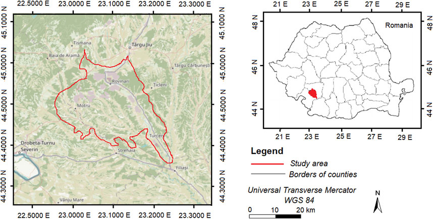
FIGURE 1. Location map of the study area.
The area’s landscape structure and land cover dynamics exhibit complex patterns. The study area comprises forests of different age classes, agricultural lands, pastures and hayfields, surface mining operations, built-up areas, dumps and water bodies. The forests contain deciduous species (sessile oak, Turkey oak and beech), mixed stands (beech, spruce and fir), coppices of alder and riparian stands along the water bodies (Tudoran, 2013). Both native species and species that have exceeded their range from the steppe to the silvo-steppe exist on meadows and hayfields (Tudoran and Zotta, 2020). Urban areas with a low density of buildings and rural areas in fragmented settlements are situated relatively close to the surface mining operations. Polluted land cover classes can also be found in the Jiului Valley due to several coal factories that existed nearby, especially before 1989.
2.2 Materials
This study used Landsat 5 TM and Landsat 8 OLI satellite images acquired during the period 1988–2017 and downloaded free of charge from the United States Geological Survey (USGS) archive (https://earthexplorer.usgs.gov/). All Landsat images were processed to L1TP-T1 level (georeferenced and orthorectified) and used the Universal Transverse Mercator (UTM) projection system, datum WGS 84, zone 34N. The images are cloud-free, acquired in a season when vegetation is present, in different years but during the same moon phase, in clear atmospheric conditions and with low noise. Using near-anniversary images reduced variations resulting from the sun angle, phenology and atmospheric condition. Information on the Landsat imagery used in this study is presented in Table 1.
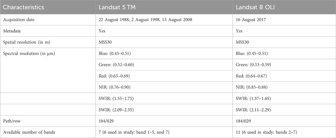
TABLE 1. Characteristics of the satellite images used in the study.
For each satellite image, cartographic materials prepared near the image acquisition date were used to assess the accuracy of the classified image. For the image acquired in 1988, the accuracy assessment was conducted based on aerial photos taken in 1986 and the cadastral maps drafted in 1986 (Vorovencii, 2021); for the 1998 image, aerial images taken in 1997 were used. The accuracy assessment of classified images from 2008 to 2017 was based on colored orthophotos (scale 1:5,000) drafted in 2008 and 2017 by the National Agency for Cadastre and Land Registration (http://geoportal.ancpi.ro/) (Vorovencii, 2021); Google Maps images and field data collection were also used for the image acquired in 2017.
The precision of the cartographic products used for the accuracy assessment depended on the precision of the instruments with which they were generated. The cadastral maps were derived from topographic maps obtained by photogrammetric stereorestitution with a precision of 0.20 mm from the drafting scale. Aerial images were taken at an approximate scale of 1:12,000. The orthophotos used have a spatial resolution of 0.5 m and a precision of 1.5 m. To ensure that the locations compared were identical, the cartographic products used for the accuracy assessment were co-registered in the same datum as the satellite images (WGS 84, zone 34N).
2.3 Image pre-processing
If two distinct features from a satellite image have the same color, discriminating between them is challenging. Differentiating and classifying the features is easier if they differ in tone or brightness (Karan and Samadder, 2016). In this study, several surface features had a similar spectral behavior on the mean signature (e.g., mined and built-up).
The downloaded images belong to the TIERS 1 category, meeting the qualitative criteria regarding geometry and radiometry. These images are considered to contain the highest quality Level-1 Precision Terrain (L1TP), suitable for analyzing land cover changes. All utilized scenes (TM and OLI) provided by USGS were georeferenced in the same projection system (UTM) within prescribed image-to-image tolerances of 12-m root mean square error (RMSE) and were used without further geometric processing. The spatial resolution of both datasets is 30 m and did not require resampling.
Due to variations in the spectral band configuration among Landsat sensors, we process only the spectral bands with corresponding wavelengths between TM and OLI sensors (Table 1). The Landsat Collection 1 data contain radiation measurements for reflective visible and infrared bands, which are depicted as scaled reflectance (OLI) or radiance (TM), recorded as integer digital numbers (DNs). We convert this data into top-of-atmosphere (TOA) reflectance, ensuring consistent scaling across all Landsat sensors. The spectral reflectance values, ranging from zero to one, were adjusted and recorded as a 16-bit unsigned integer due to the increased sensitivity of the Landsat 8 OLI sensor. Standardizing Landsat 5 TM and Landsat 8 OLI images before classification ensured bringing the data to the same scale and suitable format for classification algorithms to accurately interpret the features and variations within the images.
The images were atmospherically corrected using the dark object subtraction (DOS) method to better differentiate such features (Heumann, 2011), thus obtaining surface reflectance. This technique can reduce the additive effects caused by atmospheric haze, leading to an improved distinction between surface features. Image pre-processing and classification was conducted using ENVI, Erdas Image, and QGIS software. Figure 2 shows the overall methodology implemented in this study.
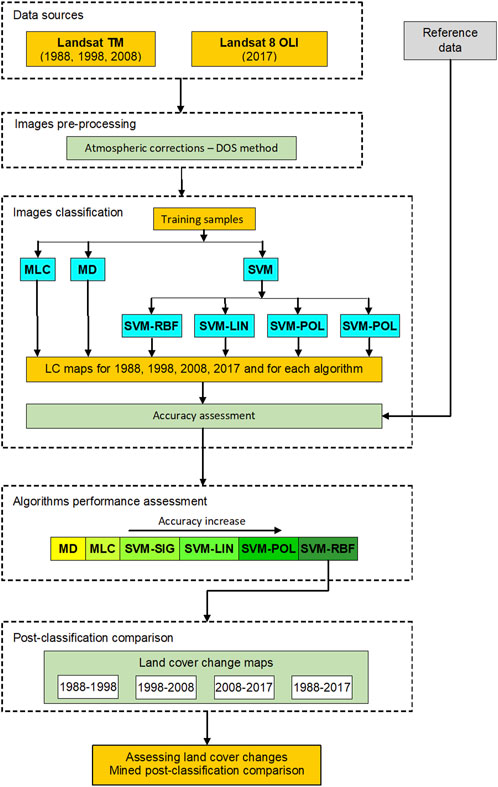
FIGURE 2. Flow of research in the classification of Landsat 5 TM and Landsat 8 OLI satellite images taken in areas with surface mining and hightlight the land cover changes.
2.4 Images classification
2.4.1 Support Vector Machine
SVMs represent a set of learning algorithms used for classification and regression. The theoretical framework was proposed by Vapnik and Chervonenkis (1971) and further developed by Vapnik (1999). SVMs are non-parametric classifiers. The result obtained by applying a SVM algorithm depends on the quality of the data training process. We consider training data, consisting of a number of samples k, represented as {Xi, yi}, i = 1, . . ., k, where
WXi + b ≥ +1 for all y = +1, for example, a member of class 1
WXi + b ≤ −1 for all y = −1, for example, a member of class 2
The two hyperplanes are chosen so as to exclude vectors and maximize the distance between two classes (Otukei and Blaschke, 2010), with the aim of attributing the new data points to a given class (Otukei and Blaschke, 2010).
SVM was initially developed to identify the linear boundaries between classes. This limitation was addressed by projecting the feature space at a large dimension under the assumption that a linear boundary can exist within a feature space with a large dimensional space (Kavzoglu and Colkesen, 2009). This projection to a higher dimensionality is commonly referred to as the kernel trick. Kernel functions used in SVMs can be broadly categorized into four groups: linear, polynomial, radial basis function and sigmoid kernels (Kavzoglu and Colkesen, 2009) (Table 2).
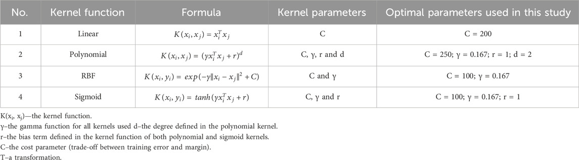
TABLE 2. SVM parameters used in the study.
Each kernel must have a different set of user-controlled parameters. These parameters consist of the cost C, the width parameter γ, the bias term r and the polynomial degree d (in the case where a polynomial kernel function is used) (Petropoulos et al., 2012). Their optimization significantly increases the accuracy of the SVM solution. The cost parameter C defines the amount of misclassification allowed for data that are inseparable from the training sample. Large values of C can lead to an over-fitting model, affecting the shape of the class-dividing hyperplane and the classification accuracy results (Melgani and Bruzzone, 2004). The kernel width parameter γ influences the smoothness of the class-dividing hyperplane’s shape (Melgani and Bruzzone, 2004). The most common polynomial degree d is 2 (quadratic) because larger degrees tend to overfit the model.
In the case of a data set, finding the optimal parameters generates the best classification (Kavzoglu and Colkesen, 2009). The grid search method is a method of choice for optimizing the parameters (Hsu et al., 2016). In the grid search method, different pairs of parameters are tested; the pair with the highest cross-validation accuracy is searched for and selected (Kavzoglu and Colkesen, 2009). The grid search method is conducted in two steps. In the first step, a coarser grid (C, γ) with an exponentially growing sequence is used (e.g., C = 2−5, 2−3 …, 215 and γ = 2−15, 2−13. . ., 23) and the cross-validation rate is calculated. In the second step, the optimal region on the grid (C, γ) is identified, a finer grid is searched for near the optimal region and a better cross-validation rate is obtained. Then, the whole training set is trained again to generate the final classifier (Kavzoglu and Colkesen, 2009; Hsu et al., 2016).
One-against-all, one-against-one and directed acyclic graph SVM (DAGSVM) strategies were developed for solving multiclass problems by applying SVM (Weston and Watkins, 1998). The one-against-all strategy divides an N-class scenario into N binary scenarios, training each model to classify one class against all others. Upon application to a test pixel, it computes a confidence value indicating the likelihood of the pixel belonging to a specific class, subsequently assigning the pixel the label of the class with the highest confidence value. However, this method confronts challenges due to potential imbalances in class sizes, which are often mitigated by duplicating samples from the smaller class. Yet, these imbalances can significantly impact the accuracy and generalization capabilities of binary SVMs (Liu et al., 2021). The one-against-one strategy generates N(N - 1)/2 classifiers, each handling a pair of classes. During testing, each classifier contributes one vote for the winning class, and the test pixel is assigned the label of the class with the most votes (Huang et al., 2002). This strategy is widely regarded as a more efficient method for multi-class classification compared to other approaches. The DAGSVM strategy aligns closely with the one-against-one method during training, utilizing N(N-1)/2 binary SVMs. However, during testing, it adopts a rooted binary directed acyclic graph structure featuring internal nodes and leaves, representing binary SVMs for each class pair. The process initiates at the root node by evaluating the binary decision function, progressing either left or right based on the output, ultimately predicting the class at a leaf node (Hsu and Lin, 2002).
The RBF kernel is widely used in SVM classification when there’s no prior knowledge about the input data. This kernel is stationary and invariant to translations, showing isotropic properties where adjusting one parameter automatically scales all others. In Table 2 (relation no. 3), the RBF kernel’s parameter γ is defined as
The discriminator function assesses whether input data is linearly separable. For the RBF kernel, the output is zero if
In this study, SVM was applied using linear (SVM-LIN), polynomial (SVM-POL), radial base function (SVM-RBF) and sigmoid (SVM-SIG) kernels. The parameters of RBF and polynomial kernels were determined by a grid search method using cross validation approach (Hsu et al., 2016). The fundamental concept underlying the grid search method is to explore diverse parameter combinations, selecting the one that achieves the highest cross-validation accuracy. Similar approaches have been utilized in previous studies involving SVM implementation (Pal and Mather, 2006; Kuemmerle et al., 2009; Petropoulos et al., 2012). Additionally, recommendations from the ENVI User’s Guide (Visual Information Solutions, 2009) regarding parameterization were also taken into consideration. For the cost C parameter, values from 0 to 500 were considered and tested for all kernels, with an increment of 50. Except for the linear kernel, the γ parameter was set to 0.167, following suggestions from the ENVI User’s Guide (Visual Information Solutions, 2009) and other studies (Petropoulos et al., 2012). For both types of images, Landsat TM and OLI, six spectral bands were used, resulting in γ = 0.167. Considering the parameter settings, combinations of cost C and the γ parameter were evaluated. For the pair that achieved the maximum overall accuracy, those respective parameters were considered optimal. The polynomial model with a degree of 2, a bias value of 1, a γ parameter of 0.167, and a cost C of 250 produced the classification result with the highest overall accuracy. The bias parameter established within the kernel function for both polynomial and sigmoid kernels was configured to a value of 1. The optimal values of these parameters are presented in Table 2.
2.4.2 Maximum likelihood
The MLC classification algorithm is based on the folowing equation (ERDAS, 1999):
where D is the weighted distance (likelihood), c represents a particular class of interest, X is the vector of spectral signature for the candidate pixel from the testing data, Mc is the mean vector of the sample of class c from the training data, ac is the percent probability that any candidate pixel is a member of class c, Covc is the covariance matrix of the pixels in the sample of class c from the training data, ǀCovcǀ is the determinant of Covc (matrix algebra), Covc−1 is the inverse Covc (matrix algebra) (Kavzoglu and Colkesen, 2009), ln is the natural logarithm function and T is the transposition function (Schrader and Pouncey, 1997; ERDAS, 1999; Mather, 2005). A pixel is assigned to class c, for which the likelihood is the highest or the least weighted distance (Kavzoglu and Colkesen, 2009).
The MLC algorithm is advantageous because it considers the variance-covariance within the class distributions (ERDAS, 1999). Assuming a normal distribution for each class, the probability of errors in the classified image is small (Kavzoglu and Reis, 2008; Kavzoglu and Colkesen, 2009).
2.4.3 Minimum distance
The MD decision rule determines the spectral distance between the measurement vector for the candidate pixel and the mean vector for each signature (ERDAS, 1999). It is simple and fast to compute, requiring only the average of the vectors for each band resulting from the sample training data. Candidate pixels are assigned to the class that is spectrally closest to the sample mean. The computation relationship is (ERDAS, 1999):
where n is the number of bands, i representsa particular band, c is a particular class, Xxyi represents the data file value of pixel x,y in band i, µci is the data file values mean in band I for the sample for class c and SDxyc is the spectral distance from pixel x,y to the mean of class c (ERDAS, 1999). After calculating the spectral distance for all possible classes, the candidate pixel is assigned to the class for which SD is the lowest (ERDAS, 1999).
2.4.4 Classification scheme and training data
The land cover classification scheme consists of seven cover classes representing the land cover in the studied area (Table 3). Six bands were used for all applied algorithms to minimize the bias caused by using different band combinations (Table 1).
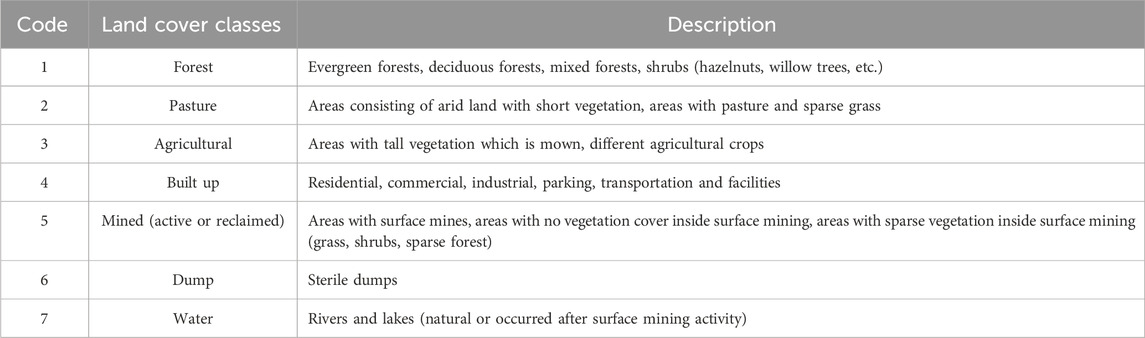
TABLE 3. Land cover classes used in satellite images classification (Vorovencii, 2021).
Training samples for spectral signatures were collected by digitizing homogeneous areas in satellite images. The samples were collected using a RGB 752 (the shortwave infrared and green bands) combination found to discriminate the land cover classes in this case. In this combination, some areas found to be polluted in the 1988 image, were more easily highlighted as part of the class they represent. The training samples were randomly selected in the known areas using ENVI software’s region of interest (ROI) tools. Part of the training samples for 2017 were collected in the field using a Trimble R8S receptor (Vorovencii, 2021). The distribution of samples was approximatively uniform and adequately covered the entire study area. The pixels included in training samples depended on the size of the land cover class; therefore, training samples included fewer pixels for less represented classes (e.g., dump, water) (Table 4). Collecting training samples for the built-up class was challenging because the area is fragmented, the built-up surfaces alternating with pasture and agricultural land. The same training samples were used for all algorithms.
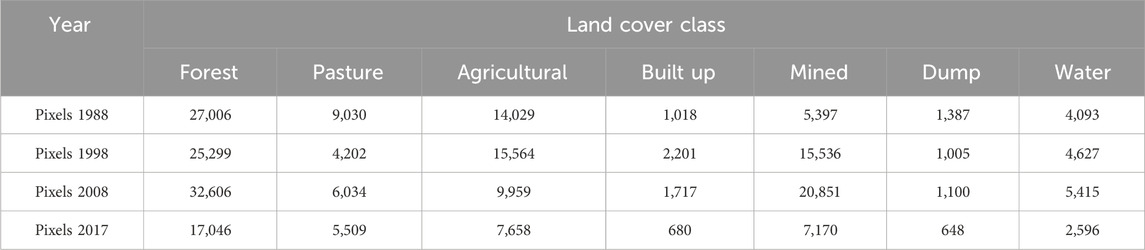
TABLE 4. Pixel counts of the training samples collected from the seven land cover classes.
2.4.5 Images classification and validation
Image classification was performed using ENVI software. The SVM classification was performed using the following kernels: linear, polynomial, RBF, and sigmoid. For each of the four SVM algorithms, the input data were satellite images, the file with previously collected spectral signatures (ROI files) and the specific optimized parameters (Table 2). Satellite images and ROI files were used as input for the MLC and MD. The same number of bands (6 bands) was used for all algorithms. Classified maps were smoothed using a 3 × 3 majority filter to minimize the ‘salt and pepper’ appearance of the images.
For the accuracy assessment, a confusion matrix was used. The overall accuracy, producer accuracy, user accuracy, quantity disagreement and allocation disagreement, instead of the Kappa coefficient (Foody, 2020), were calculated for each classified map. The overall accuracy was calculated using the following relationship (Congalton and Green, 2019):
where nii represents the number of samples classified into classes i (i = 1, 2, … , k) (Congalton and Green, 2019).
Quantity disagreement measures the absolute differences in proportions between the reference map and a comparison map of the categories (Pontius and Millones, 2011). This metric occurs when the number of pixels for each category differs in the two maps and was calculated with the following relationships (Pontius and Millones, 2011):
where, qg represents the quantity disagreement for an arbitrary category g, pig and pgi denote the estimated proportion of the arbitrary category in the simulation and reference maps, respectively, and Q represents the overall quantity.
Allocation disagreement refers to the difference between observed and simulated maps that can be atributed to variations in the spatial allocation of categories (Pontius and Millones, 2011). This accuracy metric was calculated using the following relationship (Pontius and Millones, 2011):
where, ag represents the allocation disagreement for an arbitrary category g, pgg represents the observed proportion of category g allocated to category g in the simulated map, and A represents overall allocation. Quantity disagreement and allocation disagreement together contribute to the overall disagreement D (Pontius and Millones, 2011).
Sample size planning is an imprecise science because it depends on the accuracy and information available about the analyzed area. Although this information is speculative before conducting accuracy assessment, calculating the sample size per strata can provide informative insights (Olofsson et al., 2014). To calculate the sample size, the formula applied for overall accuracy for simple random sampling and user’s accuracy for stratified random sampling was used (Stehman and Foody, 2019):
where p represents the expected overall accuracy in the case of simple random sampling or the expected user’s accuracy in the case of stratified random sampling when determining the sampling size each stratum, z is a percentile from the standard normal distribution (z = 1.96 for a 95% confidence interval), and d is the desired half-width of the confidence interval (Olofsson et al., 2014; Stehman and Foody, 2019). In the current study, stratified random sampling was adopted, with the stratum represented by thematic classes. For an expected user’s accuracy of 50%, a 95% confidence level, and 5% margin of error, a sample of 384 pixels was randomly selected from built up and mined classes. For the remaining classes, the sample size was set at 246, considering an anticipated user’s accuracy of p = 0.80. Each sample point was compared with the available reference data.
The accuracy assessment data used for validating the land cover classes were independent of the data used to train the classification (Stehman, 2009). In the case of images acquired in 1988 and 1998, the overall accuracy was limited by the low number of data available.
2.4.6 Change detection
To compare the individually classified images and obtain “from–to” information, the PCC technique was applied. Independently created land cover maps from various years were compared with PCC using a mathematical pixel-by-pixel arrangement (Toosi et al., 2019). The areas of land cover changes for the entire period were established via cross-tabulation, by subtracting the 1988 classification map from the 2017 map. The result of applying this technique was displayed as a matrix, showing the changes. In this study, the PCC technique has been used for the SVM-RBF algorithm and for four time periods: 1988–1998, 1998–2008, 2008–2017 and 1988–2017.
Change detection is particularly problematic for the accuracy assessment because it is difficult to sample areas that will undergo future changes before they occur (Congalton, 1988). Moreover, position and attribute errors can propagate in the case of multiple data, especially when more than two data are used, posing an additional problem (Yuan et al., 2005). In the present study, reference maps for the accuracy assessment of change did not exist for every period. In this regard, the same reference data were used for reference, based on which the assessment of overall accuracies was carried out for individual clasification (Olofsson et al., 2014). To assess the accuracy of the no change-changes classification, a simple size of 384 pixels was determined for each class, using stratified random sampling, considering an expected user’s accuracy of 50%, a 95% confidence level, and 5% margin of error.
3 Results
3.1 Classification results
For each of the four years in the satellite image time series, six images corresponding to the classification algorithms were obtained, generating a total of 24 classified maps (Figure 3). In each classified image, all land cover classes defined by the classification were identified. There were no unclassified pixels. Figure 4 presents the land cover analysis, with the total surface covered by each land cover class estimated by applying the algorithms.
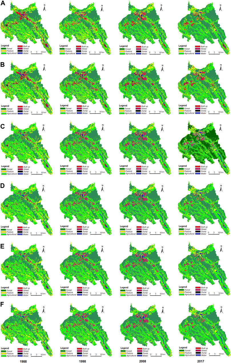
FIGURE 3. Images obtained after applying the classification algorithms: (A). MD; (B). MLC; (C). SVM-RBF; (D). SVM-LIN; (E). SVM-POL; (F). SVM-SIG.
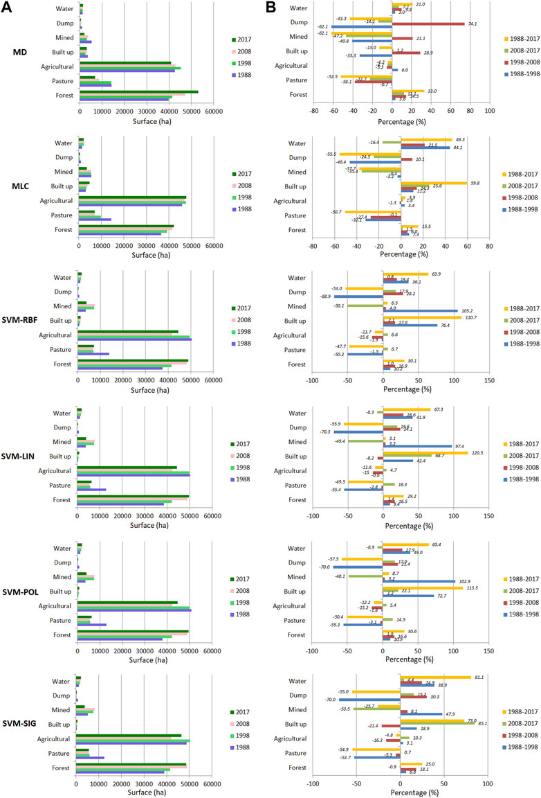
FIGURE 4. The land cover situation obtained after applying the classification algorithms (A) and the percentage differences regarding the dynamics of land cover classes for the analyzed periods (B).
The study area’s landscape is complex and the estimated surfaces differed depending on the classification algorithm. All algorithms estimated the largest surfaces in the agricultural and forest classes. The agricultural class occupied an estimated area varying between 37.9% (MD, 2017) and 47.2% (SVM-POL, 1988) of the total study area, while the forest class occupied between 33.9% (MLC, 1988) and 49.2% (MD, 2017). The pasture class covered an area of 5.2% (SVM-LIN, 2008; SVM-POL, 2008; SMV-SIG, 2008, 2017) and up to 13.3% (MLC, 1988). Although the mined and built-up classes occupied smaller areas than the agricultural, forest and pasture classes, the algorithms yielded a large range of estimates. The mined class occupied an area ranging from 1.9% (MD, 2017) to 7.6% (SVM-SIG, 2008), while the built-up class covered between 0.3% (SVM-SIG 1988; SVM-SIG 2008) and 4.5% (MLC, 2017) of the study area. The areas estimated by all algorithms as covered by water or dump were smaller than 2% and 0.9%, respectively. The surface areas estimated by the four SVM algorithms were similar, with only minor differences. In contrast, the areas estimated by the SVM algorithms and common algorithms (MLC, MD) differed considerably.
The results of the accuracy assessment using the confusion matrix are presented in Figure 5 and Figure 6. The SVM-RBF algorithm had the highest overall accuracy for all years studied, with the accuracy ranging between 86.56% (1988) and 90.68% (2017). The overall accuracies of SVMs fluctuated between 83.38% (SVM-SIG, 1988) and 90.68% (SVM-RBF, 2017). Common algorithms provided the lowest accuracy, with MD and MLC performing only slightly above 75% (minimum 76.56% for MD in 1988). The results obtained are similar to those highlighted in other studies. For example, Bouaziz et al. (2017) obtained overall accuracies of 91.20% for SVM-RBF, 90.01% for SVM-POL and only 86.00% and 78.75% for MLC and MD, respectively.
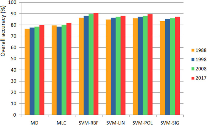
FIGURE 5. Overall accuracies of classified images.
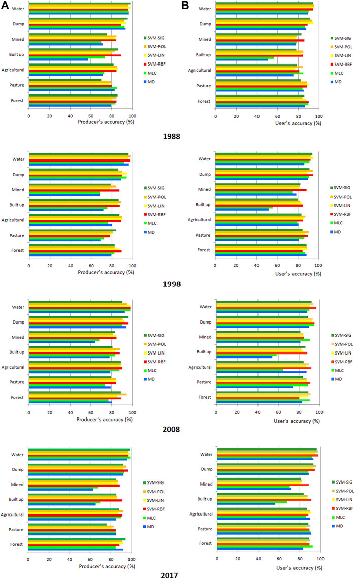
FIGURE 6. Producer’s (A) and user’s (B) accuracies of land cover classes.
In all classified images, the MD and MCL algorithms led to the lowest values for the user’s accuracy of the built-up class, with values in the range of 50.52%–67.71% (Figure 6). This means that the pixels classified on the map and ground represented the same class in this interval. The user’s accuracy of the built-up class indicated high errors of commission because other classes were highly misclassified as built-up. This resulted in a low level of discrimination on the map and an overestimation of this type of land cover (Figure 7).
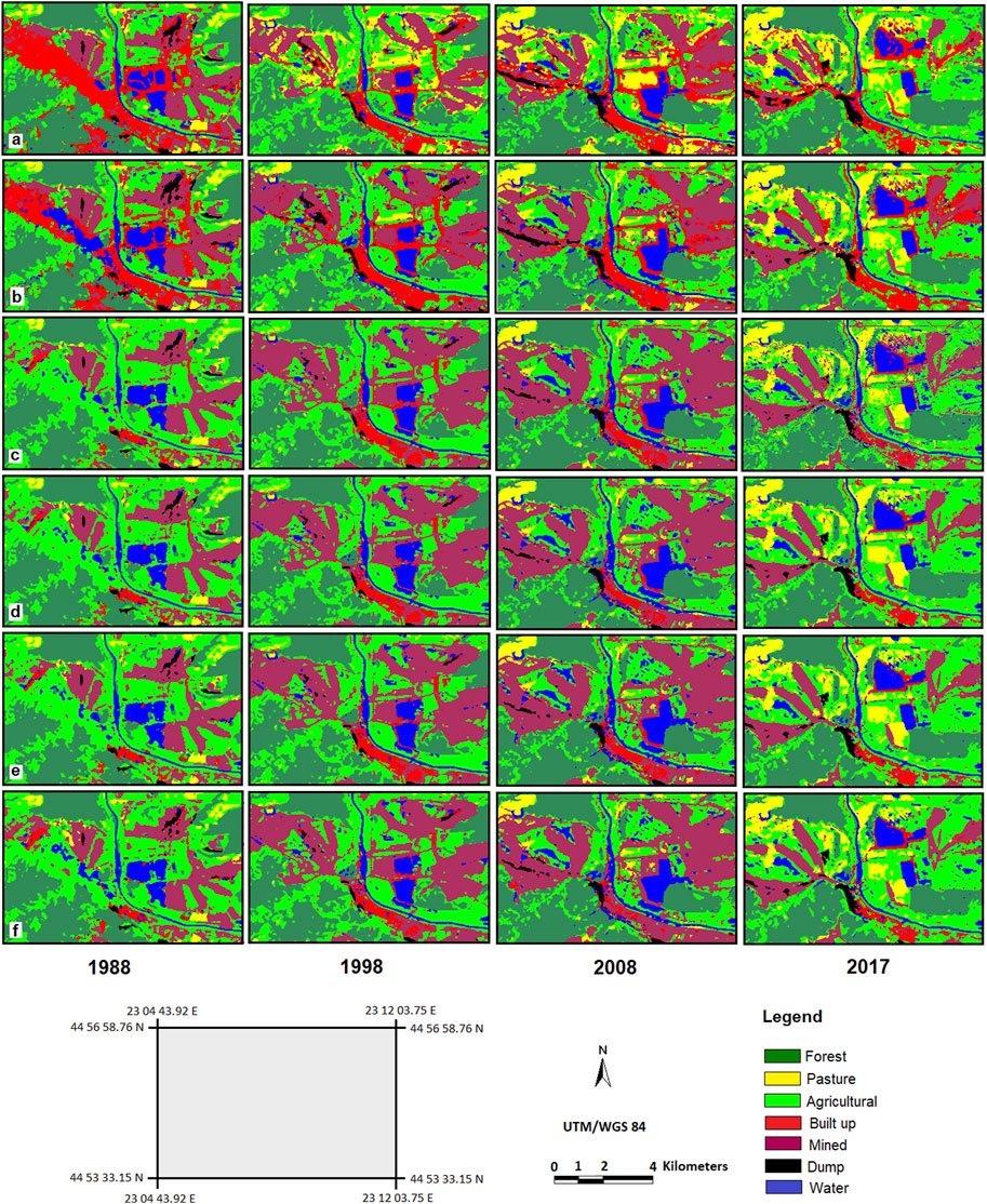
FIGURE 7. Portion of images classified by the algorithms: (A) MD; (B) MLC; (C) SVM-RBF; (D) SVM-LIN; (E) SVM-POL; (F) SVM-SIG.
In the case of the SVM algorithm, the user’s accuracy of the built-up class was between 77.67% and 90.88% for all four analyzed kernels, indicating lower errors of commission and a better separation. The producer’s accuracy for the built-up class using the MD algorithm exhibits similar results, with 57.06% in 1988 and 77.72% in 2008. In the case of the MD algorithm, both the user’s and producer’s accuracies were low for the built-up class. For example, even though 57.06% of the built-up class was identified as built-up in the 1988 image, only 50.52% were actually built-up. For the mined class, the MD and MCL algorithms produced low values (62.79%–71.25%) and, implicitly, higher omission errors. The SVM algorithm yielded producer’s accuracy values between 75.40% (mined - 1998) and 97.93% (water −2017) for all classes.
Regarding the overall disagreement, the highest values were estimated for MLC in the classification of the 2008 image (22.12%), follwed by MD (19.95%) and SVM-SIG (18.36%) in the classification of the 1988 image (Figure 8). The minimum overall disagreements were found for SVM algorithms applied to the 2008 and 2017 images. Among them, SVM-POL had a lowest values, specifically 10.10% for 2008 and 10.33% for 2017. In the case of SVM-RBF, for all analysed years, the overall disagreement ranged from 10.94% to 14.85%.
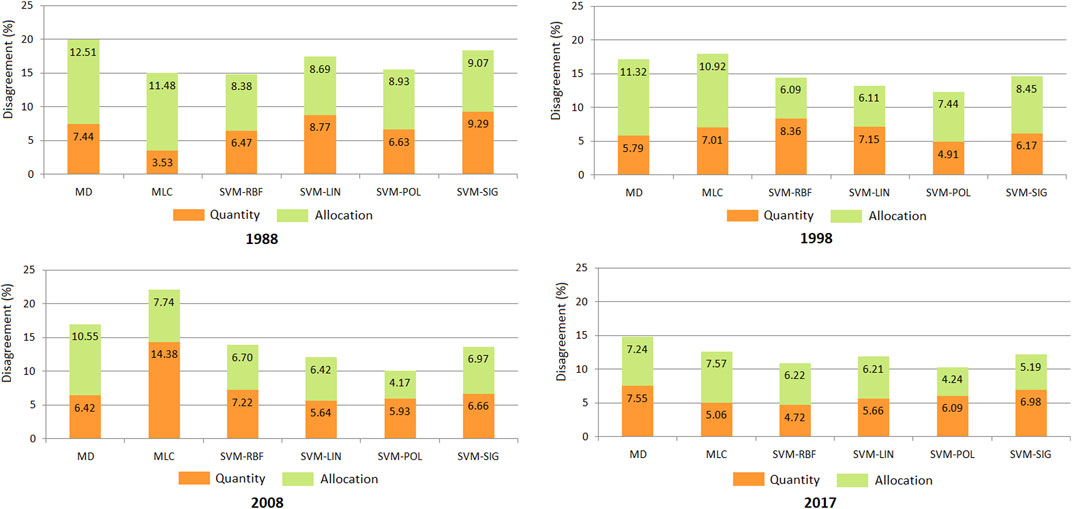
FIGURE 8. Quantity and allocation disagreement components for classification algorithms by years.
In the case of the common algorithms, the highest values for quantity and allocation disagreement were observed for all images. The highest quantity disagreement was found for the MLC algorithm (14.38% - 2008), accounting for 65.00% of the overall disagreement. High values of allocation disagreement were observed for the MD algorithm (12.51% - 1988), representing 62.71% of the overall disagreement, followed by the MLC algorithm (11.48% - 1988), accounting for 76.48% of the overall disagremement.
In the case of SVM algorithms, the values of quantity and allocation disagreements were somewhat balanced. The highest values were observed for the 1988 image, while the lowest values were found for the 2017 image. The lowest value for quantity disagreement was found for the SVM-RBF algorithm (4.72% - 2017), representing 43.14% of the overall disagreement. For allocation disagreement, the lowest value was observed for SVM-POL (4.17% - 2008), accounting for 41.29% of the overall disagreement. The highest value for quantity disagreement was estimated for the SVM-LIN algorithm (8.77%-1988), representing 50.23% of the overall disagreement, while for allocation disagreement, the SVM-SIG algorithm had the highest value (9.07% - 1988), accounting for 49.40% of the overall disagreement.
3.2 Land cover changes
Land cover changes in all analyzed periods affected all land cover classes (Figure 4). All land cover changes were obtained based on classified images showing the situation at the moment of image acquisition. The land cover changes occurred in both directions, with the land cover surface area increasing for some classes and decreasing for other classes.
The SVMs algorithms, apart from SVM-SIG, produced similar values for land cover changes. For the period 1988–2017, the difference in terms of land cover changes was 0.6% for the agricultural class, 1.4% for the forest class and 2.7% for the pasture class. Mined and built-up areas constituted the principal issue, with differences between SVM algorithms of 5.6% and 9.8%, respectively. The land cover changes estimated using the SVM-SIG algorithm differed substantially for some classes. Over the entire study period, SVM-SIG estimated a 25.7% decrease in mined areas, while the other SVMs algorithms estimated a 3.1%–8.7% increase. This constitutes a significant discrepancy in both value and direction. Indeed, on the 1988 image, SVM-SIG attributed a 5,142.8 ha area to the mined class, while SVM-RBF attributed only 3534.4 ha. For the other years, the mined area estimates were similar for all four SVMs. SVM-SIG generated a larger mined area by including the marginal areas of the mined surfaces with the other land cover classes and by classifying some small areas dispersed throughout the studied area. In addition, SVM-SIG estimated a 4.8% decrease in the agricultural class, compared to a decline of 11.6%–12.2% estimated by the other algorithms.
Common algorithms performed differently for several land cover classes, both among themselves and compared to SVMs. In the period 1988–2017, MD revealed a 62.1% decrease in the mined surface and MLC estimated a reduction of 37.7%. The built-up area estimated by MD presented a decrease of 13.0%, while MLC showed a 59.8% increase. Substantial differences were also reported in the forest class, with MD and MLC estimating increases of 33.0% and 15.5%, respectively. In the agricultural class, MD revealed a 4.2% decrease and MLC a 3.9% increase. This shows that common algorithms disagree not only on the amount but also on the direction of change.
Compared to SVMs, both common algorithms classified very large areas in the built-up class. The estimated built-up area increases between SVM-RBF and MLC were 514.6% (1988), 324.6% (1998), 317.3% (2008) and 390.3% (2017). Both common algorithms classified large built-up areas in the 1988 image near the mined area and in locations polluted by the factories existing at that time. The SVM algorithms did not significantly misclassify the land cover in these areas. In contrast, the MD and MLC algorithms generally classified smaller areas in the mined class, except for the 1988 image. For this image, MD and MLC classified mined surfaces of 5,296.9 ha and 5,563.8 ha, respectively; these areas exceed those estimated by SVM-SIG. Therefore, MD and MLC indicated a decrease in mined areas between 1988 and 2017.
The existence of mined areas located near built-up areas and especially near polluted surfaces created a complex landscape, leading to confusion between classes when passing from one class to another. Misidentification also occurred between other classes, such as forest being confused with pasture or agricultural land.
3.3 Post-classification comparison of mined areas
SVM-RBF classified images reported higher accuracy for all years; therefore, we opted to use the results from the SVM-RBF algorithm for PCC change detection. The PCC technique was applied to generate maps showing “from–to” information related to the conversions of land cover classes from analyzed periods.
The method used for accuracy assessment was described in Section 2.4.6, where 768 random samples were classified as either no-change or change class for four analyzed periods. The no-change class included all surfaces without changes, while the change class included those with changes. The overall accuracies of change detection ranged from 68.49% to 73.31% (Table 5). Over the entire period of 1988–2017, the false positive rate (false alarm), which represents the number of no-change pixels incorrectly detected as change, was 19.53%. This indicates an overestimation of the change occurrences. The false negative rate, which represents the number of change pixels incorrectly detected as no-change, was 35.16%.

TABLE 5. Change detection error matrices for 1988-1998, 1998-2008, 2008-2017, and 1988-2017 (SVM-RBF algorithm).
Table 6 presents the mined class “from–to” matrix obtained from SVM-RBF independently classified maps. This matrix indicates that estimated changes occurred in both directions: from mined class to other land cover classes (forest, pasture, etc.) and from the other land cover classes to mined class (Table 6) (Vorovencii, 2021).
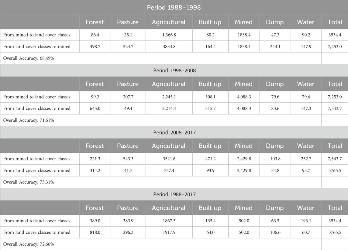
TABLE 6. “From–to” matrix (in ha) obtained through cross-tabulation of the SVM-RBF classified maps for the mined class during the periods 1988–1998, 1998–2008, 2008–2017, and 1988–2017.
The largest increase in the mined class area occurred during the period 1988–1998, corresponding to a growth of 3718.6 ha or 205.2%. During this period, 2468.0 ha (66.4%) of agricultural land, 499.6 ha (13.4%) of pasture and 412.3 ha (11.1%) of forest were converted to the mined class area, leading to this observed increase in mined land.
During the period 1998–2008, the mined class area increased by only 290.7 ha (4.0%). This modest increase results from the conversion of a large area from forest to mined land, as well as a reverse conversion from mined land to pasture. The other land cover classes (agricultural, built-up and dump) did not contribute substantially to the conversion, as areas at the end of the period remained nearly the same as at the beginning. At 4088.3 ha, the mined area was at its largest during the 1998–2008 period, as surface mining exploitation was spreading in these locations.
The period 2008–2017 is characterized by a decrease in the total mined area with 3778.2 ha (50.1%). During this period, only 92.9 ha of forest were converted to mined land, with the remaining conversions being from mined land to other classes (forest, pasture, etc.). This period saw decreased mining exploitation and several mined areas were reclaimed. The largest reclaimed surface came from converting 2764.2 ha of mined area to agricultural land and 501.6 ha to pasture. Several mined areas totaling 2429.8 ha remained during this period.
Between 1988 and 2017, mined areas increased by 6.5%, the increase being on average rather than linear. During this period, only 13.3% of the mined class remained unchanged. Conversions to and from mined areas occurred. For example, 1917.9 ha were converted from agricultural to mined land, while 1867.5 ha were converted from mined to agricultural land, as certain locations with mined areas were reclaimed and other agricultural areas were converted into surface mining operations.
4 Discussion
4.1 Accuracy assessment
A confusion matrix was used to assess algorithm accuracy on Landsat images acquired in 1988, 1998, 2008 and 2017. Result comparison revealed that the SVM-RBF algorithm provided the highest values for overall accuracy, while the MD algorithm provided the lowest values. Among the four SVM algorithms, SVM-RBF improved the overall accuracy classification by 5.99% for Landsat 5 TM and by 3.27% for Landsat 8 OLI images. These results are similar to those achieved by another study (Karan and Samadder, 2016) that found improvements of 6% and 3% for Landsat 5 and Landsat 8 images, respectively, in detecting changes in open-cast coal mining areas. We found that the SVM algorithms provided better overall accuracy than the common algorithms. More precisely, the SVM-RBF algorithm improved the overall accuracy by 10.67% compared to MD and by 8.80% compared to MLC.
The SVM algorithms exceeded MD and MLC in classifying features with similar spectral behavior encountered in the complex landscape. Using the SVMs, an improvement of up to 18.37% was observed in the mined area classification and up to 40.36% in the built-up area classification. SVM algorithms exceed MLC and MD, ensuring higher classification accuracy for each class. This is consistent with the proven high accuracy of SVMs with a small number of training samples (Karan and Samadder, 2016). In addition, Landsat 8 OLI has a higher spectral and radiometric resolution than Landsat 5 TM, resulting in an improved apparent reflectance of surface features and higher Landsat 8 OLI image accuracies for all algorithms.
The achieved accuracies in the classification resulted in various estimations of the area for each land cover class and consequently led to diverse outcomes when assessing land cover changes. Additionally, satellite images acquired at 10-year intervals might not have captured all land cover changes. Determining the time interval between satellite images from a time series depends on the characteristics of the class and the changes being assessed. Some land cover classes in the studied area may have undergone changes at shorter intervals (such as pasture, agricultural), while others occurred over longer intervals (like forest, water, etc.). Primarily focusing on the mined class, as it exhibited minimal dynamics and did not display abrupt changes between two time intervals, the interval between images was set at 10 years. Furthermore, to mitigate external factors such as sun angle and environmental characteristics, it is crucial to utilize images with anniversary or very near anniversary acquisition dates. The images utilized were acquired in different years but within close dates (from August 2nd to August 22nd) (Table 1). This approach aimed to maintain consistent image acquisition conditions and avoided selecting images from outside the specified interval. Moreover, no suitable qualitative images (e.g., without cloud cover) captured at shorter intervals were available in the USGS archive for the study area, meeting the specified conditions within the chosen intervals, thereby limiting the accuracy of our results. These considerations collectively guided the selection of images at 10-year intervals.
However, the 10-year interval between images in the time series contributed to several unexpected conversions. This might be applicable to areas where conversions between all land cover classes occurred within the same period. Some studies recommend shortening the interval between time series images (Petropoulos et al., 2012), while others advocate for a 5-year interval (Townsend et al., 2009). Nevertheless, there are specialized literature studies that have utilized satellite image time series with 10-year intervals (Kumar et al., 2021).
4.2 Algorithms performance
Using the same training samples for each land cover class allowed us to evaluate the relative performance of four advanced SVM algorithms and two common algorithms (MLC and MD) in classifying a complex landscape with surface mining from Romania’s Jiului Valley. This is very important because the accuracy of the selected algorithm as the best one determines the outcomes of the long-term changes analysis.
The slight variations in classification accuracy produced by SVMs may be attributed to the choice of the kernel function and its parameters. Considering the overall accuracies, the SVM-RBF algorithm yielded the best results, followed by SVM-POL, SVM-LIN and SVM-SIG (Figure 5). As non-linear kernels, SVM-RBF and SVM-POL may have produced better results than SVM-LIN because the class boundaries are non-linear or overlapping. Several studies using machine learning algorithms investigated different SVM parameters and demonstrated that contradictory results could be achieved (Huang et al., 2002; Foody and Mathur, 2004; Melgani and Bruzzone, 2004; Maxwell et al., 2014). For example, Melgani and Bruzzone (2004) and Maxwell et al. (2014) explored whether SVMs are robust to parameter settings. Maxwell et al. (2014) noted that parameter optimization improved classification accuracy, with only 0.1% for mining and mine reclamation mapping. Foody and Mathur (2004) demonstrated that the γ parameter significantly affected classification accuracy, with accuracies ranging from below 70% to over 90%. Similarly, Huang et al. (2002) suggested that choosing a RBF or polynomial kernel affected the shape of the decision boundary. They showed that the classification errors vary with the parameter γ when using a RBF kernel, especially when three predictor variables were used instead of seven. For the polynomial kernel, the authors determined that the classification accuracy increases with the polynomial order. Thus, the slightly different accuracies provided by SVMs in this study may result from the parameter settings, despite parameter optimization. While the best accuracy was established for the 2017 image, this accuracy may also be related to the superior characteristics of the Landsat OLI sensor compared to the Landsat 5 TM, an argument also mentioned in previous studies (Toosi et al., 2019).
The locations of each class in the classified maps were best identified by the SVM-POL algorithm applied to the 2008 image, which showed the lowest value for allocation disagreement (4.17%–41.29% of the overall disagreement). However, the quantity disagreement (5.93%–58.71% of the overall disagreement) indicate that the number of pixels perdicted for each class differs significantly from the number of reference pixels.
For the common algorithms, the number of pixels in the classified map was close to that in the reference map, resulting in low quantity disagreement. This was observed, for exemple, in the case of MLC applied to the 1988 image, where the quantity disagreement was 3.53%, and for the 2017 image, where the quantity disagreement was 5.06%. However, overall disagreement would still occur due to the assignment of pixels into the wrong class by the classifier. On the other hand, for the same algorithms and years, the allocation disagreement was 11.48% and 7.57% respectively. This indicate that many areas were classified in locations where they were not observed in the reference data. In this situation, the most commonly affected classes were built-up and mined classes.
For SVM-RBF, the disagreements due to quantity were larger than those due to allocation for 1998 and 2008. This indicate that the main disagreement between the two maps was primarily caused by errors in the quantity of the pixels rather than allocation errors. Although the overall disagreement for SVM-RBF was not the lowest, the algorithm managed to effectively separate the classes by optimizing the set parameters.
The major differences among SVM algorithms and between SVMs and the common algorithms (MLC and MD) were highlighted in the level of discrimination between mined classes and the other classes, particularly the built-up class (Figure 7). The SVM algorithms, principally SVM-RBF, have been better at discriminating between mined and built-up areas without major difficulties in learning the support vectors. However, the complex characteristics of built-up areas contrast with the high homogeneity of agricultural, forest or pasture areas, which posed intrinsic classification difficulties for SVMs as well. Fringe areas, characterized by alternating built-up land and agricultural land or pasture, presented such a challenge. In the presence of fringe areas, the classification accuracy for built-up areas remained inferior to that of agricultural areas, an aspect also observed in other studies (Xu et al., 2010; Myint et al., 2011; Ma et al., 2017).
Therefore, the primary challenge was distinguishing mined areas from built-up areas. In many areas, mined land was classified as built-up and vice versa. This error was especially common in marginal, transitional areas between land cover classes. The built-up class had a low user’s accuracy with the MD and MLC algorithms (Figure 6); it was sometimes mistaken for other classes due to the similarity of its spectral features and small height variances (Vorovencii, 2021). The built-up class included urban areas with a spectral reflectance similar to that of bare soil and rocks (Vorovencii, 2021). In the case of rural areas, built-up areas alternated with areas occupied by courtyards and gardens, giving the area a fringed aspect and making built-up land difficult to distinguish from agricultural land. The moderate spatial resolution of the Landsat images (30 m) enhanced this effect, further lowering the likelihood of adequately differentiating these classes.
The two common algorithms produced classification errors overestimating the built-up surface at the expense of mined areas for all years, especially in 1988 (Figure 6). In 1988, large areas were polluted due to local factories; these areas were classified as built-up in the 1988 image (Figures 7A,B). The MD and MLC algorithms generated the weakest results for these areas, mistaking the polluted surfaces covered with vegetation for built-up or mined areas.
The MD algorithm depends solely on the mean vector for each spectral class and does not use covariance information. This algorithm performs better when the variance in the data is low. However, the pixel values representing the polluted surfaces above the built-up areas and near them in the 1988 image resulted in a significantly split high variance. Therefore, the MD algorithm did not perform well compared to the MLC algorithm for the built-up class (Figure 4). Ganasri et al. (2014) obtained similar results for the period 2007–2013, when an increase of 4.8% and a decrease of 44.3% were obtained for the urban area by applying the MLC and MD algorithms, respectively.
All algorithms produced some classification errors between forest, pasture and agricultural classes. In some locations, mined areas were classified as pasture or agricultural land. This type of errors frequently occurred in marginal zones, transitional areas between different land classes, particularly in places where a reclaimed mine is situated. The algorithms SVM-POL, SVM-LIN and SVM-SIG slightly underestimated the built-up areas and slightly overestimated the mined areas. Although both MD and MLC algorithms overestimated built-up areas, MLC highlighted linear details, such as paved roads, better than MD (especially in the 2008 image). The SVMs algorithms identified part of these linear details as mined areas.
The accuracy sensitivity of the SVM classifications to training set size indicates the need to include outlying cases for the training set, yielding adequate support vectors. Although SVMs do not require a large training sample set to estimate the statistical distribution, the training sample must include useful support vectors that adequately define the class boundaries (Foody and Mathur, 2004). The probability of finding useful support vectors is higher in a large training sample than in a small sample (Foody and Mathur, 2004). The training set size was smaller for the mined and built-up classes considering the smaller area they occupy and their distribution in the study area. A larger training sample set would have increased the probability of including mixed pixels. Results confirm that a balanced sample size is preferable.
The quality of the training data impacts the accuracy of the SVMs. Foody et al. (2016) noted that SVM accuracy dropped by 8% when 20% of the training data were mislabeled, emphasizing that training data quality is essential even for robust algorithms. The accuracy of the MLC and MD algorithms also depended on the quality of the training data. It is possible that the training data given was not entirely qualitative. Land was classified as mined or built-up areas where the probability of including mixed pixels in the training sample was high. Mixed pixels are common in Landsat data due to the heterogeneity of the landscape and the fact that the data’s spatial resolution is limited to 30 m. By using only the features’ spectral signature, the existence of a large number of mixed pixels in a training sample could lead to its deterioration. Under these conditions, mixed spectral pixels can negatively impact the classification results generated via MLC or MD.
In an imbalanced training dataset, classes with limited representation across the study area often exhibit lower accuracies. The disparity in coverage between built-up, mined areas, and the forest class within our study area might lead to varied performance of MD and MLC algorithms. For instance, in the 1988 image, the built-up area accounts for 1.64% of the experimental area, mined areas for 8.71%, while the forest area covers 43.59%. This means that the training samples for the built-up area represent only one twenty-sixth of the forest area samples, while the training samples for mined areas represent one-fifth. In the 2017 image, the built-up area represents 1.65%, while the forest covers 41.27% of the experimental area, indicating one twenty-fifth of the forest area samples. Data augmentation and training tuning could serve as methods to improve the performance of MD and MLC.
In the present study, the number of training samples may have been sufficient for SVMs but insufficient for the common algorithms, which contributed to their poor accuracy. Indeed, some studies suggest that SVMs require fewer training samples than common algorithms (Foody and Mathur, 2004). In this study, the training sample sets were larger for the forest, pasture and agricultural classes and smaller for the other land cover classes. The 1988 image was associated with the largest errors for the MD and MLC algorithms. For this image, the training samples represented 15.7% and 13.7% of the built-up and mined areas classified by SVM-RBF (considered as a reference), respectively; this may not have been sufficient for MD and MLC. The weight of training samples was higher for the 1998 and 2008 images, where the SVMs algorithms estimated mined and built-up surfaces with higher accuracy. For the 1998 image, training samples represented 19.3% of the mined class and 19.2% of the built-up class. For the 2008 image, they represented 24.9% of the mined class and 12.8% of the built-up class. Therefore, the percentage of training samples compared to the occupied surface significantly affects the classification accuracy. Some studies have noted that the training data can indeed have a greater impact than the choice of algorithm (Huang et al., 2002).
Some studies suggest that SVM algorithms are insensitive to data sizes, increases or decreases of band numbers taken into the classification, and thus, that accuracy is independent of the number of bands (Pal and Mather, 2006). Other studies show that the classification accuracy using SVMs increases when the number of bands included in the classification decreases (Weston et al., 2000). The present study did not investigate the effect of the number of bands on classification accuracy. The analysis focused solely on the six optical bands aimed to assess and emphasize primary spectral features and their influence on classification. Furthermore, the study specifically examined temporal changes in spectral data, without incorporating additional data that might have offered a more spatial perspective rather than temporal. However, we can posit that the number of bands used (6 bands) was too small to be a decisive factor for classification accuracy for common algorithms.
Parametric classifiers assume that the data is representative and normally distributed. However, most data collected in the field do not follow any typical model (e.g., Gaussian mixture, linearly separable), which is also the case with land cover classes. As such parametric classifiers, MD and MLC provided poor accuracy because the land cover data was not normally distributed, the landscape being heterogeneous and complex. In addition, the land cover surface distribution could not be described based on data distribution as it exhibited a high level of uncertainty. In these situations, non-parametric SVM algorithms yielded superior results.
Providing the weakest accuracy, the MD algorithm did not consider the classes’ variability; this resulted in wide differences among the classes’ variances and led to misclassifications. When the landscape is complex, the parametric classifiers often produce ‘noisy’ results (Lu and Weng, 2007). Moreover, the MD algorithm computed faster than SVM algorithms due to its mathematical simplicity, as it only required mean vectors for each band in the training data.
The classification algorithms used in this study present both advantages and disadvantages. Thus, the MD algorithm has proven to be simple, fast, and works well when land cover classes exhibit good discrimination in the feature space. However, the algorithm is sensitive to variations and data interferences, making it less efficient in classifying data without a clear distribution. Additionally, in cases of multidimensional data or data that does not separate well in the feature space, its performance decreases. On the other hand, MLC is well-grounded theoretically, having the ability to handle data with a more complex, non-uniform distribution or with class overlap. Nevertheless, it is sensitive to sample size, meaning its performance is affected when using small samples. Also, with large datasets, it requires increased computational power. Regarding SVMs, their advantage lies in their ability to perform well in multidimensional spaces. By utilizing various kernels, they adopt complex decision functions and can prevent overfitting. Furthermore, they are not as sensitive to sample size and can work with smaller samples. However, SVMs are sensitive to kernel selection, which means their performance is influenced by the correct choice of the kernel and the establishment of optimal parameters. Also, training an SVM model may require more time, especially with large datasets or when using complex kernels. Therefore, each classification algorithm has both strengths and limitations, and the choice of an algorithm crucially depends on the specific objectives of the study, the nature of the data, and the specific characteristics of the landscape.
4.3 Assessment of land cover changes
In addition to the results regarding map changes, the results highlighted a 231.1 ha increase in surface mining in the study area over the entire 1988–2017 period. The fluctuation in the surface area subjected to surface mining during these three decades was high, registering two peaks in the first two periods (1988–1998 and 1998–2008), followed by a decrease in the third period (2008–2017). These two peaks correlate with the transition from underground mining to surface mining that occurred after 1989, a transition that significantly degraded the landscape in the area (Vorovencii, 2021). The relief was modified by new forms, both positive (sterile dumps) and negative (remaining quarry pits) (Fodor and Lazăr, 2006; Vorovencii, 2021). The hydrological processes were affected by the removal of the topsoil and vegetation cover by surface mining activity. The area experienced changes in the quality and quantity of surface and underground water, landslides and various geomechanical phenomena such as subsidence (Fodor and Lazăr, 2006).
The profound changes observed during the study period are linked to Romania’s socio-economic upheaval after 1989. These changes touched all sectors of the economy through the transition from a centralized economy to a market economy. An important factor is the application of land laws, which aimed to restore property rights but also led to the fragmentation of forests and agricultural lands. In the period 1988–2017, the forest class increased by 30.1% through the expansion of trees and shrubs at the expense of pasture, which decreased by 47.7%. The phenomenon followed the neglect of the pastures after 1989, which were invaded by various shrub and tree species. The agricultural class saw a decrease of 11.7% as the lands were no longer worked due to a decreasing interest in agriculture. Inadequate government policies regarding agricultural development were responsible for this decline. New landowners did not own agricultural machinery or owned inefficient machinery, resulting in low productivity. The move from large-scale agricultural exploitations to small or very small areas exploited by different owners also contributed to the decrease in agricultural land. The built-up class experienced the largest growth over the entire study period, particularly during the 1988–1998 subperiod. The reason for this growth is two-fold: first, the construction sector underwent considerable growth after 1989; secondly, numerous areas like riverbeds were misclassified as asphalt or concrete areas. However, the built-up area decreased between 2008 and 2017 stands in contrast to the general upward trend observed in built-up areas throughout the entire period. This decrease is likely a result of including pixels from various classes, notably those from the mined class, within the samples designated as built-up. Romania joined the European Community in 2007, and new environmental protection regulations were imposed that reduced mining activity. As a result, numerous employees lost their jobs and moved to other localities. The dump class decreased by 53% after 1988, a decrease explained by their covering with grassy and shrubby vegetation and some re-greening operations of surface mining areas.
4.4 Remarks to the study
The obtained results are specific to Romania’s Jiului Valley mining basin. The possibility of generalizing the conclusions to other studies conducted in regions with similar or dissimilar landscapes depends on the specificities of these landscapes. This specificity can be influenced by numerous factors, such as landscape structure, its unique characteristics, human activities in the area, different geographical or ecological variables that might be unique. Additionally, aspects related to the methodology used, dataset specifics, algorithm peculiarities, and data collection methods need to be considered.
Identifying regions with geographic, ecological characteristics, and land cover classes similar to those in the Jiului Valley mining basin is crucial. For landscapes with similar characteristics, the conclusions drawn from this study might be applicable. However, for landscapes with heterogeneity, diverse land cover types, intense human activities, high ecological diversity, and substantial altitude variations, generalizing the results and conclusions poses a significant challenge. In such regions, the optimal algorithms and parameters identified in this study might not be as effective or suitable. In these circumstances, for SVMs, parameter tuning becomes crucial to match the specifics of these landscapes and ensure high accuracy and result relevance in a new context. For common algorithms, the challenge lies in the quality and quantity of data used for training and testing.
Moreover, adapting these algorithms and methodologies in regions with dissimilar landscapes might require additional resources such as more detailed field data, satellite images with superior spatial, radiometric, and spectral resolutions, and local expertise. Assessing the availability of these resources can influence the practical applicability of methodologies in other regions. Additionally, applying the methodology in other regions with different landscapes necessitates conducting additional field tests and validations to evaluate the effectiveness and generalization of the conclusions. Comparing the obtained results with field data and other information sources strengthens confidence in generalizing the findings.
Examining how the findings of this study correspond to the prerequisites and aims of particular domains (such as environmental conservation and natural resource management) in diverse regions is crucial to evaluate the usefulness and significance of the outcames. In conclusion, although this study might provide relevant information regarding land cover classification, highlighting, and assessing land cover changes in Romania’s Jiului Valley mining basin, the direct applicability of conclusions to other regions with similar or dissimilar landscapes requires a more careful approach and adequate adaptation.
5 Conclusion
Highlighting and assessing the long-term changes in the complex landscape with surface mining from Jiului Valley, Romania, during the period of 1988–2017, was achieved by pursuing two specific objectives. The first objective, integral to the adopted method for highlighting land cover changes, involved mapping land cover classes within the study area using multiple classification algorithms. Using the same training data set, Landsat satellite images were classified, resulting in various levels of accuracy. The ability of SVM algorithms to generate an optimal separating hyperplane led to improved performance compared to the MD and MLC algorithms. The accuracies varied slightly among the four SVM algorithms, and SVM-RBF performed best. The final results depended on the chosen kernel, the optimization of the selected kernel parameters and the method used to generate the SVM. An accuracy assessment based on the confusion matrix revealed that SVM algorithms produce more accurate estimates for classes with overlapping spectral reflectance values on the signature plot. Among the common algorithms, MLC performed better than MD. However, common algorithms give less reliable results than SVMs for complex landscapes. Both common and advanced algorithms operate at the pixel level rather than the sub-pixel level, possibly resulting in lower accuracy due to mixed pixels when using medium spatial resolution satellite images.
The second objective was to highlight and assess the land cover changes in surface mining areas over a 29-year period. The assessment was conducted based on the results obtained from SVM-RBF algorithm, as it ensured the best accuracy. The PCC technique was used to obtain change maps and “from–to” information. Results suggest that detecting changes from satellite images in a complex landscape is a complicate process, requiring a unique approach applicable to all cases. During the study period, mined areas increased on average by 6.5%, with considerable increases and decreases in the intermediate periods. The transition from underground to surface mining was the main driving force behind this change. The expansion of surface mining affected the landscape by changing the area’s relief and degrading the ecological balance.
This study analyzes the long-term changes in Jiului Valley’s mining landscape, shedding light on Romania’s shift from underground to surface mining post-1989 and its socio-economic impacts. The results provide valuable insights into the relationship between socio-economic shifts and land cover, aiding future research and land management strategies in analogous settings. Emphasizing the significance of assessing land cover changes in complex mining landscapes, the study highlights the role of satellite imagery and machine learning algorithms, particularly SVM, in ensuring accurate evaluations. It underscores the use of satellite images over time as a key tool for understanding human environmental impact and prioritizes monitoring land cover changes to aid surface mining activities and area reclamation.
To enhance the assessment of land cover changes, future research will concentrate on utilizing images from new satellite programs and data collected by unmanned aerial vehicles to depict analyzed features more distinctly. For instance, we can utilize satellite imagery from Copernicus programs such as radar images from Sentinel-1 and optical images from Sentinel-2, the latter having a spatial resolution of 10 m, as well as satellite images from Planet, which offer a spatial resolution of 3.7 m. Additionally, the exploration will involve the adoption of new, more effective classification algorithms like machine learning and deep learning, along with the utilization of alternative metrics for assessing classification accuracy. Among machine learning algorithms, successful candidates may include RF, Gradient Tree Boosting (GTB), k-NN, while deep learning algorithms such as Convolutional Neural Networks (CNNs), Recurrent Neural Networks (RNNs), U-Net will also be examined. Furthermore, we aim to integrate texture features, topographic details, vegetation indices, and other non-spectral information into machine learning algorithms to further enhance their performance in satellite image classification. Consequently, the grey level co-occurrence matrix (GLCM) may be employed to extract texture features like entropy, variance, correlation, contrast, homogeneity, etc. Topographic data represented by digital elevation model, slope, and aspect can significantly contribute to improving classification accuracy, particularly in areas where vegetation is altitude-dependent. Vegetation indices selection will be tailored based on the study’s objectives, landscape nature, and land cover types. Other non-spectral data that could be utilized encompass climatic or meteorological data, geographical and socio-economic information, or additional supplementary data sources.
Data availability statement
The original contributions presented in the study are included in the article, further inquiries can be directed to the corresponding author.
Author contributions
IV: Conceptualization, Data curation, Formal Analysis, Investigation, Methodology, Supervision, Validation, Writing–original draft, Writing–review and editing.
Funding
The author declare financial support was received for the research, authorship, and/or publication of this article. This work has been supported for publication by Transilvania University of Brasov.
Acknowledgments
We would like to thank the USGS website for the Landsat imagery, Transilvania University of Brașov for the aerial photos, the National Agency for Cadastre and Land Registration for the colour orthophotos, and Trimble Inc. for the Trimble R8S receptor and the Trimble Business Center educational software. Also, we thank to reviews for the observations made that determined the quality improvment of the article.
Conflict of interest
The author declares that the research was conducted in the absence of any commercial or financial relationships that could be construed as a potential conflict of interest.
Publisher’s note
All claims expressed in this article are solely those of the authors and do not necessarily represent those of their affiliated organizations, or those of the publisher, the editors and the reviewers. Any product that may be evaluated in this article, or claim that may be made by its manufacturer, is not guaranteed or endorsed by the publisher.
References
Adelabu, S., Mutanga, O., and Adam, E. (2014). Evaluating the impact of red-edge band from Rapideye image for classifying insect defoliation levels. ISPRS J. Photogramm. Remote Sens. 95, 34–41. doi:10.1016/j.isprsjprs.2014.05.013
Albatal, R., and Little, S. (2014). Empirical exploration of extreme SVM-RBF parameter values for visual object classification. Lect. Notes Comput. Sci. Incl. Subser. Lect. Notes Artif. Intell. Lect. Notes Bioinforma. 8326 LNCS, 299–306. doi:10.1007/978-3-319-04117-9_28
Batta, P., Singh, M., Li, Z., Ding, Q., and Trajkovic, L. (2018). Evaluation of support vector machine kernels for detecting network anomalies. Proc. - IEEE Int. Symp. Circuits Syst. 2018. doi:10.1109/ISCAS.2018.8351647
Bayarsaikhan, U., Boldgiv, B., Kim, K. R., Park, K. A., and Lee, D. (2009). Change detection and classification of land cover at Hustai National Park in Mongolia. Int. J. Appl. Earth Obs. Geoinf. 11, 273–280. doi:10.1016/j.jag.2009.03.004
Bouaziz, M., Eisold, S., and Guermaz, E. (2017). Semiautomatic approach for land cover classification: a remote sensing study for arid climate in southeastern Tunisia. Euro-Mediterranean J. Environ. Integr. 2, 24. doi:10.1007/s41207-017-0036-7
Castellana, L., D’Addabbo, A., and Pasquariello, G. (2007). A composed supervised/unsupervised approach to improve change detection from remote sensing. Pattern Recognit. Lett. 28, 405–413. doi:10.1016/j.patrec.2006.08.010
Chaves, M. E. D., Picoli, M. C. A., and Sanches, I. D. (2020). Recent applications of Landsat 8/OLI and Sentinel-2/MSI for land use and land cover mapping: a systematic review. Remote Sens. 12, 3062. doi:10.3390/rs12183062
Chen, W., Li, X., and Wang, L. (2020). Fine land cover classification in an open pit mining area using optimized support vector machine and world view-3 imagery. Remote Sens. 12, 82–14. doi:10.3390/RS12010082
Cihlar, J. (2000). Land cover mapping of large areas from satellites: status and research priorities. Int. J. Remote Sens. 21, 1093–1114. doi:10.1080/014311600210092
Congalton, R. G. (1988). A comparison of sampling schemes used in generating error matrices for assessing the accuracy of maps generated from remotely sensed data. Photogramm. Eng. Remote Sens. 54, 593–600.
Congalton, R. G., and Green, K. (2019). Assessing the accuracy of remotely sensed data. Principles and Practices. 3th ed. USA: CRC Press.
DeFries, R. S., and Chan, J. C. W. (2000). Multiple criteria for evaluating machine learning algorithms for land cover classification from satellite data. Remote Sens. Environ. 74, 503–515. doi:10.1016/s0034-4257(00)00142-5
Demirel, N., Emil, M. K., and Duzgun, H. S. (2011). Surface coal mine area monitoring using multi-temporal high-resolution satellite imagery. Int. J. Coal Geol. 86, 3–11. doi:10.1016/j.coal.2010.11.010
Dietterich, T. G. (1998). Approximate statistical tests for comparing supervised classification learning algorithms. Neural comput. 10, 1895–1923. doi:10.1162/089976698300017197
Esmail, M., Masria, A., and Negm, A. (2016). Monitoring land use/land cover changes around damietta promontory, Egypt, using RS/GIS. Procedia Eng. 154, 936–942. doi:10.1016/j.proeng.2016.07.515
Fodor, D., and Lazăr, M. (2006). Ecological occupation and rehabilitation of land in the Oltenia area (in Romanian). AGIR Bull. 3, 27–31.
Foody, G. M. (1986). Approaches for the production and evaluation of fuzzy land cover classifications from remotely-sensed data. Int. J. Remote Sens. 17, 1317–1340. doi:10.1080/01431169608948706
Foody, G. M. (2020). Explaining the unsuitability of the kappa coefficient in the assessment and comparison of the accuracy of thematic maps obtained by image classification. Remote Sens. Environ. 239, 111630. doi:10.1016/j.rse.2019.111630
Foody, G. M., and Mathur, H. (2004). A relative evaluation of multiclass image classification by Support Vector Machines. IEEE Trans. Geosci. Remote Sens. 42, 1335–1343. doi:10.1109/tgrs.2004.827257
Foody, G. M., Pal, M., Rocchini, D., Garzon-Lopez, C. X., and Bastin, L. (2016). The sensitivity of mapping methods to reference data quality: training supervised image classifications with imperfect reference data. ISPRS Int. J. Geo-Information 5, 199. doi:10.3390/ijgi5110199
Fraser, R. H., Olthof, I., and Pouliot, D. (2009). Monitoring land cover change and ecological integrity in Canada’s national parks. Remote Sens. Environ. 113, 1397–1409. doi:10.1016/j.rse.2008.06.019
Ganasri, B. P., Arun, A. M., Praveer, R., Srirsm, S., and Dwarakish, G. S. (2014). “Analysing land use and land cover change pattern using classification techniques in Harangi catchment, Karnataka State, India,” in Proceedings of the 19th IAHR-APD congress 2014 (Hanoi, Vietnam: IAHR-APD).
Gresita, C. I. (2011). Expert system used for monitoring the behaviour of hydrotechnical constructions. REVCAD J. Geod. Cadastre 11, 75–84.
Gresita, L. (2013). Surveying methods to studying the behaviour of dams (in Romanian). Iasi: Tehnopress Publishing House.
Guebert, M. D., and Gardner, T. W. (1989). Unsupervised SPOT classification and infiltration rates on surface mined watersheds, central Pennsylvania. Photogramm. Eng. Remote Sens. 55, 1479–1486.
Hall, F. G., John, R. T., and Engman, E. T. (1995). Status of remote sensing algorithms for estimation of land surface state parameters. Remote Sens. Environ. 51, 138–156. doi:10.1016/0034-4257(94)00071-t
Hay, G. J., Blaschke, T., Marceau, D. J., and Bouchard, A. (2003). A comparison of three image-object methods for the multiscale analysis of landscape structure. ISPRS J. Photogramm. Remote Sens. 57, 327–345. doi:10.1016/S0924-2716(02)00162-4
Heumann, B. W. (2011). An object-based classification of mangroves using a hybrid decision tree-support vector machine approach. Remote Sens. 3, 2440–2460. doi:10.3390/rs3112440
Hsu, C. W., Chang, C. C., and Lin, C. J. (2016). A practical guide to support vector classification. Taipei: Taiwan.
Hsu, C. W., and Lin, C. J. (2002). A comparison of methods for multiclass support vector machines. IEEE Trans. Neural Netw. 13, 415–425. doi:10.1109/72.991427
Huang, C., Davis, L. S., and Townshend, J. R. G. (2002). An assessment of support vector machines for land cover classification. Int. J. Remote Sens. 23, 725–749. doi:10.1080/01431160110040323
Karan, S. K., and Samadder, S. R. (2016). Accuracy of land use change detection using support vector machine and maximum likelihood techniques for open-cast coal mining areas. Environ. Monit. Assess. 188, 486. doi:10.1007/s10661-016-5494-x
Karan, S. K., and Samadder, S. R. (2018a). A comparison of different land-use classification techniques for accurate monitoring of degraded coal-mining areas. Environ. Earth Sci. 77, 713–715. doi:10.1007/s12665-018-7893-5
Karan, S. K., and Samadder, S. R. (2018b). Improving accuracy of long-termland-use change in coal mining areas using wavelets and Support Vector Machines. Int. J. Remote Sens. 39, 84–100. doi:10.1080/01431161.2017.1381355
Kavzoglu, T., and Colkesen, I. (2009). A kernel functions analysis for support vector machines for land cover classification. Int. J. Appl. Earth Obs. Geoinf. 11, 352–359. doi:10.1016/j.jag.2009.06.002
Kavzoglu, T., and Reis, S. (2008). Performance analysis of maximum likelihood and artificial neural network classifiers for training sets with mixed pixels. GIScience Remote Sens. 45, 330–342. doi:10.2747/1548-1603.45.3.330
Khatami, R., Mountrakis, G., and Stehman, S. V. (2016). A meta-analysis of remote sensing research on supervised pixel-based land-cover image classification processes: general guidelines for practitioners and future research. Remote Sens. Environ. 177, 89–100. doi:10.1016/j.rse.2016.02.028
Kuemmerle, T., Chaskovskyy, O., Knorn, J., Radeloff, V. C., Kruhlov, I., Keeton, W. S., et al. (2009). Forest cover change and illegal logging in the Ukrainian Carpathians in the transition period from 1988 to 2007. Remote Sens. Environ. 113, 1194–1207. doi:10.1016/j.rse.2009.02.006
Kumar, P., Dobriyal, M., Kale, A., and Pandey, A. K. (2021). Temporal dynamics change of land use/land cover in Jhansi district of Uttar Pradesh over past 20 years using LANDSAT TM, ETM+ and OLI sensors. Remote Sens. Appl. Soc. Environ. 23, 100579. doi:10.1016/j.rsase.2021.100579
Lawrence, R., Bunn, A., Powell, S., and Zambon, M. (2004). Classification of remotely sensed imagery using stochastic gradient boosting as a refinement of classification tree analysis. Remote Sens. Environ. 90, 331–336. doi:10.1016/j.rse.2004.01.007
Lillesand, T. M., and Kiefer, R. W. (1999). Remote sensing and image interpretation. New York: John Wiley and Sons Ltd.
Liu, L., Martín-Barragán, B., and Prieto, F. J. (2021). A projection multi-objective SVM method for multi-class classification. Comput. Ind. Eng. 158, 107425. doi:10.1016/j.cie.2021.107425
Löw, F., Michel, U., Dech, S., and Conrad, C. (2013). Impact of feature selection on the accuracy and spatial uncertainty of per-field crop classification using Support Vector Machines. ISPRS J. Photogramm. Remote Sens. 85, 102–119. doi:10.1016/j.isprsjprs.2013.08.007
Lu, D., Mausel, P., Batistella, M., and Moran, E. (2004). Comparison of land-cover classification methods in the Brazilian Amazon basin. Photogramm. Eng. Remote Sens. 70, 723–731. doi:10.14358/PERS.70.6.723
Lu, D., and Weng, Q. (2007). A survey of image classification methods and techniques for improving classification performance. Int. J. Remote Sens. 28, 823–870. doi:10.1080/01431160600746456
Lucieer, V. (2008). Object-oriented classification of sidescan sonar data for mapping benthic marine habitats. Int. J. Remote Sens. 29, 905–921. doi:10.1080/01431160701311309
Ma, L., Li, M., Ma, X., Cheng, L., Du, P., and Liu, Y. (2017). A review of supervised object-based land-cover image classification. ISPRS J. Photogramm. Remote Sens. 130, 277–293. doi:10.1016/j.isprsjprs.2017.06.001
Mantero, P., Moser, G., and Serpico, S. B. (2005). Partially supervised classification of remote sensing images through SVM-based probability density estimation. IEEE Trans. Geosci. Remote Sens. 43, 559–570. doi:10.1109/tgrs.2004.842022
Mather, P. M. (2005). Computer processing of remotely sensed images: an introduction. 3rd Editio. China: John Wiley and Sons Ltd.
Maxwell, A. E., Warner, T. A., Strager, M. P., and Pal, M. (2014). Combining RapidEye satellite imagery and lidar for mapping of mining and mine reclamation. Photogramm. Eng. Remote Sens. 80, 179–189. doi:10.14358/PERS.80.2.179-189
Melgani, F., and Bruzzone, L. (2004). Classification of hyperspectral remote sensing images with support vector machines. IEEE Trans. Geosci. Remote Sens. 42, 1778–1790. doi:10.1109/TGRS.2004.831865
Mitra, P., Uma Shankar, B., and Pal, S. K. (2004). Segmentation of multispectral remote sensing images using active support vector machines. Pattern Recognit. Lett. 25, 1067–1074. doi:10.1016/j.patrec.2004.03.004
Mundia, C. N., and Aniya, M. (2005). Analysis of land use/cover changes and urban expansion of Nairobi city using remote sensing and GIS. Int. J. Remote Sens. 26, 2831–2849. doi:10.1080/01431160500117865
Myint, S. W., Gober, P., Brazel, A., Grossman-Clarke, S., and Weng, Q. (2011). Per-pixel vs. object-based classification of urban land cover extraction using high spatial resolution imagery. Remote Sens. Environ. 115, 1145–1161. doi:10.1016/j.rse.2010.12.017
Nyamekye, C., Ghansah, B., Agyapong, E., and Kwofie, S. (2021). Mapping changes in artisanal and small-scale mining (ASM) landscape using machine and deep learning algorithms. - a proxy evaluation of the 2017 ban on ASM in Ghana. Environ. Challenges 3, 100053. doi:10.1016/j.envc.2021.100053
Olofsson, P., Foody, G. M., Herold, M., Stehman, S. V., Woodcock, C. E., and Wulder, M. A. (2014). Good practices for estimating area and assessing accuracy of land change. Remote Sens. Environ. 148, 42–57. doi:10.1016/j.rse.2014.02.015
Osuna, E., Freund, R., and Girosi, F. (1997). An improved training algorithm for support vector machines. in Neural Networks for Signal Processing VII. Proceedings of the 1997. New York: IEEE Workshop, 276–285.
Otukei, J. R., and Blaschke, T. (2010). Land cover change assessment using decision trees, support vector machines and maximum likelihood classification algorithms. Int. J. Appl. Earth Obs. Geoinf. 12, S27–S31. doi:10.1016/j.jag.2009.11.002
Pal, M. (2012). “Advanced algorithms for land use and cover classification,” in Advances in mapping from remote sensor imagery. Editor J. Li (New York: CRC Press), 69–90.
Pal, M., and Mather, P. M. (2003). An assessment of the effectiveness of decision tree methods for land cover classification. Remote Sens. Environ. 86, 554–565. doi:10.1016/S0034-4257(03)00132-9
Pal, M., and Mather, P. M. (2006). Some issues in the classification of DAIS hyperspectral data. Int. J. Remote Sens. 105, 2895–2916. doi:10.1080/01431160500185227
Petropoulos, G., Partsinevelos, P., and Mitraka, Z. (2012). Change detection of surface mining activity and reclamation based on a machine learning approach of multitemporal Landsat TM imagery. Geocarto Int. 28, 323–342. doi:10.1080/10106049.2012.706648
Pôças, I., Cunha, M., Marcal, A. R. S., and Pereira, L. S. (2011). An evaluation of changes in a mountainous rural landscape of Northeast Portugal using remotely sensed data. Landsc. Urban Plan. 101, 253–261. doi:10.1016/j.landurbplan.2011.02.030
Pontius, R. G., and Millones, M. (2011). Death to Kappa: birth of quantity disagreement and allocation disagreement for accuracy assessment. Int. J. Remote Sens. 32, 4407–4429. doi:10.1080/01431161.2011.552923
Praticò, S., Solano, F., Di Fazio, S., and Modica, G. (2021). Machine learning classification of mediterranean forest habitats in google earth engine based on seasonal sentinel-2 time-series and input image composition optimisation. Remote Sens. 13, 586–628. doi:10.3390/rs13040586
Richards, J. A. (2013). Remote sensing digital image analysis: an introduction. 2nd Editio. Heidelberg: Springer Berlin. doi:10.1007/978-3-642-30062-2
Rodriguez-Galiano, V. F., Ghimire, B., Rogan, J., Chica-Olmo, M., and Rigol-Sanchez, J. P. (2012). An assessment of the effectiveness of a random forest classifier for land-cover classification. ISPRS J. Photogramm. Remote Sens. 67, 93–104. doi:10.1016/j.isprsjprs.2011.11.002
Rogan, J., Franklin, J., Stow, D., Miller, J., Woodcock, C., and Roberts, D. (2008). Mapping land-cover modifications over large areas: a comparison of machine learning algorithms. Remote Sens. Environ. 112, 2272–2283. doi:10.1016/j.rse.2007.10.004
Rogan, J., and Miller, J. (2006). “Integrating GIS and remotely sensed data for mapping forest disturbance and change,” in Understanding forest disturbance and spatial pattern: remote Sensing and GIS approaches. Editors S. E. Wulder, and Franklin (New York: CRC Press), 133–172.
Roscher, R., Förstner, W., and Waske, B. (2012). I2VM: incremental import vector machines. Image Vis. comput. 30, 263–278. doi:10.1016/j.imavis.2012.04.004
Sabins, F. F. (1997). Remote sensing. Principles and interpretation. 3th Editio. New York: W.H. Freeman and Company.
Shao, Y., and Lunetta, R. S. (2012). Comparison of support vector machine, neural network, and CART algorithms for the land-cover classification using limited training data points. ISPRS J. Photogramm. Remote Sens. 70, 78–87. doi:10.1016/j.isprsjprs.2012.04.001
Stehman, S. V. (2009). Sampling designs for accuracy assessment of land cover. Int. J. Remote Sens. 30, 5243–5272. doi:10.1080/01431160903131000
Stehman, S. V., and Foody, G. M. (2019). Key issues in rigorous accuracy assessment of land cover products. Remote Sens. Environ. 231, 111199. doi:10.1016/j.rse.2019.05.018
Szuster, B. W., Chen, Q., and Borger, M. (2011). A comparison of classification techniques to support land cover and land use analysis in tropical coastal zones. Appl. Geogr. 31, 525–532. doi:10.1016/j.apgeog.2010.11.007
Tigges, J., Lakes, T., and Hostert, P. (2013). Urban vegetation classification: benefits of multitemporal RapidEye satellite data. Remote Sens. Environ. 136, 66–75. doi:10.1016/j.rse.2013.05.001
Toosi, N. B., Soffianian, A. R., Fakheran, S., Pourmanafi, S., Ginzler, C., and Waser, L. T. (2019). Comparing different classification algorithms for monitoring mangrove cover changes in southern Iran. Glob. Ecol. Conserv. 19, e00662. doi:10.1016/j.gecco.2019.e00662
Townsend, P. A., Helmers, D. P., Kingdon, C. C., McNeil, B. E., de Beurs, K. M., and Eshleman, K. N. (2009). Changes in the extent of surface mining and reclamation in the Central Appalachians detected using a 1976–2006 Landsat time series. Remote Sens. Environ. 113, 62–72. doi:10.1016/j.rse.2008.08.012
Townshend, J. R. (1992). Land cover. Int. J. Remote Sens. 13, 1319–1328. doi:10.1080/01431169208904193
Tudoran, G. M. (2013). Regulations regarding the management of forests included in natural protected areas. Bull. Transilv. Univ. Braşov, Ser. II For. Wood.Industry. Agric. Food Eng. 55, 35–38.
Tudoran, G. M., and Zotta, M. (2020). Adapting the planning and management of Norway spruce forests in mountain areas of Romania to environmental conditions including climate change. Sci. Total Environ. 698, 133761. doi:10.1016/j.scitotenv.2019.133761
Ustuner, M., Sanli, F. B., and Dixon, B. (2015). Application of support vector machines for landuse classification using high-resolution rapideye images: a sensitivity analysis. Eur. J. Remote Sens. 48, 403–422. doi:10.5721/EuJRS20154823
Vapnik, W. N. (1999). An overview of statistical learning theory. IEEE Trans. Neural Netw. 10, 988–999. doi:10.1109/72.788640
Vapnik, W. N., and Chervonenkis, A. Y. (1971). On the uniform convergence of the relative frequencies of events to their probabilities. Theory Probab. its Appl. 17, 264–280.
Visual Information Solutions, I. (2009). ENVI user’s Guide restricted rights notice. Available at: www.apache.org/.
Vorovencii, I. (2021). Changes detected in the extent of surface mining and reclamation using multitemporal Landsat imagery: a case study of Jiu Valley, Romania. Env. Monit. Assess. 193, 30. Available at:. doi:10.1007/s10661-020-08834-w
Vorovencii, I., and Muntean, D. (2012). Evaluation of supervised classification algorithms for Landsat 5 TM images. RevCAD; J. Geod. Cadas. 11, 229–238.
Wahla, S. S., Kazmi, J. H., and Tariq, A. (2023). Mapping and monitoring of spatio-temporal land use and land cover changes and relationship with normalized satellite indices and driving factors. Geol. Ecol. Landscapes 00, 1–17. doi:10.1080/24749508.2023.2187567
Weston, J., Mukherjee, S., Chapelle, O., Pontil, M., Poggio, T., and Vapnik, V. (2000). MIT open access articles feature selection for SVMs feature selection for SVMs.
Xu, H. Q., Li, P. J., Zhang, Y., Wang, J. F., and Coops, N. C. (2010). Urban land cover classification from very high resolution imagery using spectral and invariant moment shape information. Can. J. Remote Sens. 36, 248–260. doi:10.5589/m10-042
Yuan, F., Sawaya, K. E., Loeffelholz, B. C., and Bauer, M. E. (2005). Land cover classification and change analysis of the Twin Cities (Minnesota) metropolitan area by multitemporal Landsat remote sensing. Remote Sens. Environ. 98, 317–328. doi:10.1016/j.rse.2005.08.006
Keywords: support vector machine, maximum likelihood, minimum distance, machine learning algorithm, Landsat, land cover changes
Citation: Vorovencii I (2024) Long-term land cover changes assessment in the Jiului Valley mining basin in Romania. Front. Environ. Sci. 12:1320009. doi: 10.3389/fenvs.2024.1320009
Received: 11 October 2023; Accepted: 08 January 2024;
Published: 22 January 2024.
Edited by:
Juergen Pilz, University of Klagenfurt, AustriaReviewed by:
Kwame Oppong Hackman, West African Science Service Centre on Climate Change and Adapted Land Use (WASCAL), Burkina FasoMario Cunha, University of Porto, Portugal
Fan Mo, Ministry of Natural Resources of the People’s Republic of China, China
Copyright © 2024 Vorovencii. This is an open-access article distributed under the terms of the Creative Commons Attribution License (CC BY). The use, distribution or reproduction in other forums is permitted, provided the original author(s) and the copyright owner(s) are credited and that the original publication in this journal is cited, in accordance with accepted academic practice. No use, distribution or reproduction is permitted which does not comply with these terms.
*Correspondence: Iosif Vorovencii, aW9zaWYudm9yb3ZlbmNpaUB1bml0YnYucm8=