 Lucas Alencar
 Maria Isabel Sobral Escada
 José Luís Campana Camargo2
- 1Laboratory of Applied Ecology, Biosciences Centre, Department of Botany, Federal University of Pernambuco, Recife, Brazil
- 2Biological Dynamics of Forest Fragments Project, Department of Ecology, National Institute for Amazon Research, Manaus, Brazil
- 3General Coordination of Earth Observation, Image Processing Division, National Institute for Space Research, São Paulo, Brazil
Secondary vegetation is increasingly recognized as a key element for biodiversity conservation and carbon stocks in human-modified landscapes. Contrasting deforestation patterns should lead to distinct patterns of forest regeneration, but this relationship is yet to be unveiled for long-term studies. Using Landsat data from 1985–2015, we analyzed the surface area, spatial distribution, and age of secondary vegetation in Fishbone and Geometric patterns of deforestation. Additionally, we investigated to which extent secondary vegetation reduces forest patch isolation at the landscape level across time. We found the Fishbone pattern to consistently have more secondary vegetation over time than the Geometric pattern, despite having the same size of the deforested area. However, the Fishbone pattern showed more secondary vegetation area with less than 5 years old, while the Geometric pattern showed more area with secondary vegetation with more than 30 years old. Regarding spatial distribution, we found secondary vegetation to be more spread across the entire landscape at the Fishbone pattern and to consistently reduce forest patch isolation across time. This is congruent with the land use typically found in Geometric (industrial cropping and ranching) and Fishbone (fallow agriculture with small-scale ranching) patterns. These findings indicate that the Fishbone pattern of deforestation produces a more biodiversity-friendly landscape structure than the Geometric pattern. On the other hand, older secondary vegetation found in the Geometric deforestation pattern could indicate more carbon stocked in those landscapes. Future public policies of land use and occupation should consider better landscape planning and management to overcome this duality and create synergies between biodiversity conservation and secondary vegetation carbon stock.
1 Introduction
Secondary vegetation has an increasing role in landscape planning and management to face current climate and biodiversity crises, offsetting some of the most pervasive consequences of deforestation. Secondary vegetation is currently recognized as an important sink of carbon dioxide (Jones et al., 2019; Hall et al., 2022), a regulator of local climate (Lee et al., 2021; van Meerveld et al., 2021), and a water systems stabilizer (van Meerveld et al., 2021). It also has an important role in biodiversity conservation, since secondary vegetation recovers part of the taxonomic and functional diversity and habitat structure (Poorter et al., 2021). Secondary vegetation is considered an (increasingly) important component of tropical landscapes (Arroyo-Rodríguez et al., 2017). In the Amazon forest, for example, estimates of secondary vegetation area vary from 13.3 MHa (27% of total deforested area in 2018) (MapBiomas 2022) to 14.9 MHa (or 30% in 2018) (Silva Junior et al., 2020). However, this vegetation is under threat due to the recent increase in deforestation, fostering of non-sustainable activities in the Amazon rainforest, and changes in governmental strategies to combat deforestation (Atkins and Menga 2021). The effects of deforestation on the temporal and spatial dynamics of secondary vegetation are unclear, but it is crucial to understand this relationship to plan for its sustainable use.
The occupation process of the Amazon was heterogeneous and carried by different actors supported by distinct public policies at different time frames, generating a variety of deforestation patterns (Silva et al., 2008; Alves et al., 2021). Each leaves a specific footprint of deforestation, generating a variety of landscape configurations (i.e., different forest patch sizes, numbers, shapes, and locations) (Mertens and Lambin 1997; Saito et al., 2011). In the Amazon, several patterns of deforestation have already been identified (Mertens and Lambin 1997; Geist and Lambin 2002; Silva et al., 2008; Saito et al., 2011; Arima et al., 2015), however, there are two historically important and commonly found patterns in the region: the Geometric and the Fishbone pattern. The Geometric pattern is commonly associated with large-scale cattle ranching and industrialized commodity production. This pattern is characterized by deforestation in large areas with geometric shapes (often above 1,000 ha) and intensive land use, through mechanized and capitalized large-scale agribusiness (Saito et al., 2011; Arima et al., 2015). Whereas the Fishbone pattern is associated with conventional rural settlement as performed by the Brazilian National Institute of Colonization and Agrarian Reform (INCRA) during the 1970s and 1980s. This pattern is characterized by small irregular polygons of deforestation (INCRAS´s lot size varies from 25–100 ha) located near secondary roads, connected transversely to a main road, creating a deforestation pattern that resembles a fishbone. It is also associated with small-scale family farming usually with lower mechanized and capitalized agricultural practices (Saito et al., 2011; Alencar et al., 2016).
Deforestation changes the spatial arrangement of landscape elements (e.g., shifts patches of forest size and area) (Prist et al., 2012) which can result in fragmented landscapes that affect forest regeneration. Forest regeneration is the process in which a cleared area is able to restore to a new forest cover (i.e., secondary vegetation) without any human interference along the process (Chazdon 2012). In fragmented landscapes, the speed of forest regeneration and biodiversity recovery varies with landscape configuration. Small and isolated patches, for example, are typically absent of animals and tend to attract less seed dispersers that are fundamental for forest regeneration (San-José et al., 2020), decreasing plant functional connectivity (Auffret et al., 2017). Another fundamental aspect influencing natural regeneration of forests is land use history (Mesquita et al., 2015; Arroyo-Rodríguez et al., 2017; Poorter et al., 2021). Estimates from models of forest regeneration in tropical regions that were logged and burned point to a slow recovery rate of above ground biomass (De Faria et al., 2020). High intensity fires typically destroy the seed bank, and kill seedlings and saplings, changing the course of community assemblage and stalling the natural regeneration process (Mesquita et al., 2015). Therefore, the different actors and land management approaches in Geometric and Fishbone patterns may affect forest regrowth differently across time and space, since each pattern imprints a specific configuration to landscape elements.
If not persistently burned, a regenerating forest can recover part of the vegetation cover and the landscape structure lost to deforestation (Chazdon 2012; Laurance et al., 2018). Beyond gains in vegetation cover, naturally regenerating secondary vegetation may contribute to increase in landscape connectivity (Molin et al., 2018). Species movement tends to be high in more permissive matrices, such as secondary vegetation (Eycott et al., 2012). For this reason, even in fragmented landscapes meta-communities and meta-populations can still be connected (Watling et al., 2011), maintaining genetic flow (Ribeiro et al., 2021) and decreasing the risk of local species extinction (Chase et al., 2020). The positive effects are stronger when the secondary vegetation grows to late successional stages (Tabarelli et al., 2012; Carrara et al., 2015). Thus, evaluating the long-term impacts of contrasting deforestation patterns (Geometric and Fishbone) over forest regeneration is paramount to understand patterns of natural regeneration and how it may over time mitigate the negative impacts of deforestation on landscapes.
Therefore, we aim to answer the following questions: 1) How do Geometric and Fishbone deforestation patterns affect the extent and the spatial configuration of the secondary vegetation patches in the Amazonian landscape? 2) How does growing secondary vegetation reduce forest patch isolation over time? 3) How do contrasting deforestation processes affect the persistence of secondary vegetation in landscapes? Our hypotheses are: 1) Geometric deforestation patterns should be less favorable for secondary vegetation growth and lead to a patchy distribution of secondary vegetation, due to intensive use of land; 2) Secondary vegetation should strongly reduce the isolation of forest patches in landscapes with Fishbone deforestation patterns, since fallow agriculture (common practice in INCRA settlements and family farming) allows forest regeneration in several parts of the deforested land, spreading secondary vegetation across the landscape; and 3) Secondary vegetation in the Fishbone pattern of deforestation should be more persistent, as farmers in small rural settlements in general utilize less mechanized agricultural practices.
2 Materials and methods
2.1 Landscape selection
Among several existing deforestation patterns (see Saito et al., 2011), we choose to evaluate the forest regeneration process in the Geometric and Fishbone patterns, since they are the outcome of two distinct public policies and land occupation strategies in the Brazilian Amazon. The Geometric footprint happened after the establishment of a land occupation policy to attract large cattle ranchers to southern Amazon during the 1970s and 1980s (Hoelle 2014). This policy offered tax incentives and guaranteed land ownership conditioned to farmers maintaining land productivity (Fearnside 2005). Therefore, most of the landscapes in the Amazon with this type of footprint are located in the Southern part of Rondônia, Mato Grosso and Pará states (Figure 1). The Amazonian occupation strategy that created the Fishbone pattern had a similar philosophy of “bringing people to non-populated areas” offering incentives, such as rural credit and technical assistance, while imposing obligations, to prohibit the resale of land and ensure farm productivity (Alencar et al., 2016). However, this policy was focused on small-scale family farmers and happened in different places in the Amazon. Most of the landscapes with this footprint are found in northern Rondônia, Mato Grosso and Pará, and also in Acre and Roraima states (Figure 1). Those patterns are easily detected and identified by visual inspection of satellite images, such as the ones generated by the Landsat series (Mertens and Lambin 1999; Oliveira Filho and Metzger 2006). The identification of deforestation patterns was carried out visually considering criteria such as shape, size, edges, and the spatial arrangement of deforested patches observed in Landsat images over time. The two selected deforestation patterns (fishbone and geometric) are well known in the tropical forest literature and described by Mertens and Lambin (1997), Silva et al. (2008); Saito et al. (2011); Arima et al. (2015). The geometric deforestation pattern corresponds to large deforested patches, with geometric shape, compact and well-defined forest/non-forest edges. The fishbone pattern is defined mainly by the distinct spatial arrangement of the small regular deforestation patches, located specifically in INCRA’s planned Settlement Project. In these areas, the lots are organized alongside local roads arranged orthogonally to the axis of the main road. The typical occupation of the lots (and deforestation) starts from the road to the end generating the easily recognizable fishbone footprint in satellite images.
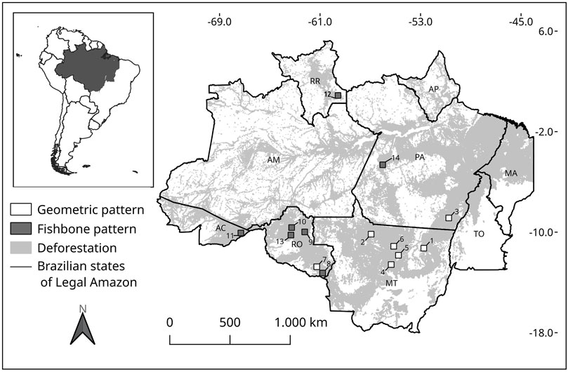
FIGURE 1. Location of fourteen 50 × 50 km landscapes with either Fishbone or Geometric pattern of deforestation. Light gray shade is the cumulative deforestation in Legal Amazon from 1985–2015. Numbers connected to boxes indicate the landscape identification. Brazilian geopolitical division (states) in the Legal Amazon: AC–Acre; AM–Amazonas; RO–Rondônia; RR–Roraima; MT–Mato Grosso; PA–Pará; AP–Amapá; TO–Tocantins; MA–part of Maranhão.
We built a multitemporal database with images from Landsat-5 and Landsat-8 (at 30 m spatial resolution) from 1985–2015, collected in intervals of 5 years. The Landsat scenes were obtained from USGS’s Earth Explorer system (United States Geological Survey (USGS) 2019). To delimit the landscapes, we choose 50 × 50 km areas in the Landsat scenes with Geometric or Fishbone patterns. The landscape size was chosen based on recommendations from Saito et al. (2011) who showed a better stability of landscape metrics in the Amazon region. We selected 12 landscapes for each deforestation pattern, with around 80% of forest cover at the beginning of the analysis period (1985) and at least 5% of deforested area. With this threshold, it is already possible to clearly identify the deforestation pattern through visual inspection of the Landsat images. In areas with a lower proportion of deforestation in 1985 (i.e., around 5%), we evaluated the evolution of the landscape using the multi-temporal image data from Landsat series until the year 2015 (the last year of our analysis) to confirm the pattern. We only chose the landscapes that maintained either the Geometric or the fishbone pattern of deforestation. Then, we removed landscapes with any levels of cloud cover, image noises and other elements that could mislead image classification, such as areas of non-forest physiognomy (e.g., enclaves of savanna, known as Cerrado or the open, shrub-dominated areas known as Campinas), large rivers, etc. As a result, seven sites remained in the analysis for each pattern in the selected years, resulting in 98 landscapes of 50 × 50 km (Figure 1).
2.2 Image classification
We only classify landscapes with forest formation, considered as all vegetation formation with forest phytophysiognomy observed in the Landsat images. Landscapes that presented natural vegetation with non-forest phytophysiognomy were removed from the analysis. Our definition of forest areas may include classes of open or dense ombrophilous forest, and seasonal decidual forest (e.g., in the southern region of Legal Amazon). To identify the areas of old growth forest and deforestation inside those landscapes, we built a Linear Spectral Mixing Model to split the images using their soil, shadow, and vegetation fractions. This technique is used to highlight certain types of targets and to reduce the dimensionality of the data (Shimabukuro and Smith 1991). We chose to use soil fraction as a feature to the image classification process based on the procedures established by Almeida et al. (2010) and the TerraClass project (Almeida et al., 2016). Then we performed a Segmentation by Region Growth algorithm using the SPRING software (Câmara et al., 1996). This segmentation groups the pixels of the imagens according to their gray levels (similarity threshold) and form clusters of a minimum size (area threshold). We empirically defined the similarity and area threshold in 8 and 16 pixels, respectively. Afterwards, we used an unsupervised classification algorithm, Isoseg (Bins et al., 1993) implemented in the software SPRING 5.5.1 (Câmara et al., 1996) by region. According to Bins et al. (1993) Isoseg is a clustering technique applied to a set of regions obtained from a segmented image, based on an acceptance threshold and on a number of classes defined by the user. We empirically choose an acceptance threshold of 95% and two classes. The segmentation step, splits the image into regions and extracts their statistical attributes (mean, covariance matrix and area). The regions are ordered by size and classified with the clustering algorithm considering the covariance matrix and the mean vector of the regions to estimate the centers of the classes. The regions whose means lie within the maximum Mahanalobis distance defined from the center of the class are considered as belonging to it. For the detection of the initial classes, the statistical parameters of the first region of the list are taken as initial parameters of a certain class. In an interactive process, all regions with a Mahalanobis distance of a certain class lower than the acceptance threshold are removed from the list. Statistical parameters are recalculated and this operation is repeated until no more regions are removed from the list. If the number of detected classes is greater than the number initially defined, the classes with the smallest number of regions are removed and the regions are classified for the remaining classes using the Mahalanobis distance criterion. One of the major advantages of using Isoseg, which is an approach based on regions and not on pixels, is the definition of the initial centroids based on existent statistical information (extracted from image during the segmentation process) and the use of the Mahalanobis distance for assigning labels. It increases the probability of having a lower intraclass variance and a higher interclass variance, providing a better distinction among the classes (Bins et al., 1993). In the end, the clusters can be regrouped manually considering the classes of interest. In this study the obtained clusters were grouped to forest and non-forest classes, according to the land cover they represent.
To identify secondary vegetation in deforested areas we used the soil fraction feature and defined thresholds empirically to slice the images and identify this land cover class. In this step we applied a deforestation mask (built on images from previously year) to restrict the classification area reducing confusion between secondary vegetation and old growth forest. We added areas classified as secondary vegetation to the maps of forest/non-forest, obtaining final maps with three land cover classes: old growth forest, secondary vegetation and deforestation. We visually inspected the maps and manually edited misclassified areas. We emphasize that this strictly remote sensing procedure hinders the inference about the structure and composition of the secondary vegetation mapped. Therefore, we generically denoted areas under recovery as secondary vegetation, which includes several stages of forest regeneration (Almeida et al., 2016).
2.3 Landscape metrics and data analysis
Landscape metrics are spatial measures of landscape structure and composition (Wang et al., 2014) used in the context of this study to analyze classes of land cover and their spatial arrangements and composition. These metrics allows to evaluate size, shape, dominance, diversity, connection, isolation, and abundance of land cover classes (McGarigal 2015). When measured over time, these metrics may reveal the landscape fragmentation process and the potential long-term consequences on biodiversity (Rosa et al., 2017). These metrics provide valuable information to biodiversity and conservation biology researchers. Therefore, we chose landscape metrics that can reveal configuration changes in the landscape over time and we discuss how these changes can directly and indirectly affect biodiversity conservation within these landscapes (Carrara et al., 2015; Rocha et al., 2016). We used the FRAGSTATS v4.2 (McGarigal 2015) software to calculate all landscape metrics.
First, we calculated the initial percentage of old growth forest cover in all selected landscapes, which allowed us to check whether the level of deforestation was similar for both studied patterns across time. This enabled the evaluation of trajectories for both landscape types (i.e., Geometric and Fishbone) from the same starting point. Furthermore, isolating the effect of the deforestation amount in each set of landscapes from the pattern in which the landscapes have been cleared. For each year, we performed the non-parametric test of Mann-Whitney (Hart 2001) to compare the total amount of forest cover in landscapes with a Geometric pattern of deforestation versus landscapes with the Fishbone. Additionally, we performed an Analysis of Covariance (ANCOVA), using the deforestation pattern as covariate and time as explanatory variable, to check if the rate of secondary vegetation growth (i.e., slope of the linear model) differ between Geometric and Fishbone patterns.
We used the Clumpiness Index (CLUMPY) to measure the distribution of the secondary vegetation on the landscape. This metric evaluates the spatial aggregation of a given type of land cover and follows the formula,
where gii is the number of pixels with adjacent pixels belonging to the same cover class, gik is the number of pixels with adjacent pixels that belong to a different type of cover, i = 2 (relative to secondary vegetation cover class); k = 0 or 1 (relative to deforested areas of old-growth forests, respectively). The second formula shows that the CLUMPY metric depends on the relationship between Gi and Pi, where Pi is the proportion of the landscape occupied by the chosen analyzed class. The value of CLUMPY ranges from −1 to 1; the closer to -1, the more disaggregated are the patches of the type land cover evaluated; on the contrary, the closer to 1, the greater the spatial aggregation of the patches; and if closer to zero, the patches are randomly dispersed across the landscape (McGarigal 2015). We compared the landscapes within each year using the Mann-Whitney test (Hart 2001).
To measure the effect of secondary vegetation over the isolation between forest fragments, we first measured the mean isolation of the old growth forest fragments using the Euclidean nearest neighbor distance mean (ENN_MN) (McGarigal 2015). This landscape metric calculates the Euclidean distance between one patch and its closest neighbor and then average them out for the landscape. It ranges from greater than 0 up to the maximum distance inside the limits of the landscape. After measuring the distance using only the fragments of old growth forest, we then recalculated the metric considering the secondary vegetation. Then, we calculated the mean reduction of ENN_MN when including the secondary vegetation.
To evaluate the persistence of the secondary vegetation in both deforestation patterns, we used images from 2015 as the reference, because it represents the “end of the process” of deforestation and occupation over 30 years (1985–2015). Note that, due to our mapping analysis approach, i.e., data collected every 5 years, we could not precisely define the age of the secondary vegetation. However, we checked the occurrence of the secondary vegetation in previous years and classified them into six categories of age (up to 5 years old, 5–10, 10–15, 15–20, 20–25 and 25–30 years old). Then, we measured the secondary vegetation patch area of each age category. For example, for secondary vegetation in the 20–25 years old category, we considered every area that was present in 1990 and in all subsequent years up to 2015, but not in 1985. Note that, our definition of age is an estimate based on the persistency of that area of secondary vegetation observed in the classified landscapes during the study period. Thus, some areas of secondary vegetation may be more than 30 years old (25–30 years old category), since the oldest analyzed image is from 1985. Another limitation is due to the 5-years interval used, since some areas of secondary vegetation may have been cut and regenerated within this period.
3 Results
3.1 Mapping forest cover
We classified a total of 98 landscapes from two contrasting deforestation patterns (seven from Geometric and seven from Fishbone) from 1985–2015. Our method rendered thematic maps for each landscape (in each time point) with three land cover classes: old growth forest, secondary forest and non-forest (Supplementary Figure S1; Figure 2). Table 1 presents a summary of the differences we found between Geometric and Fishbone pattern using our set of landscape metrics.
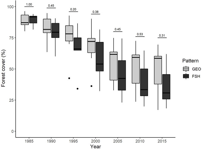
FIGURE 2. Changes in old growth forest cover in landscapes with two distinct deforestation patterns in the Brazilian Amazon. GEO–Geometric pattern of deforestation. FSH–Fishbone pattern of deforestation. The numbers above boxplots correspond to the p-value of Mann-Whitney test.
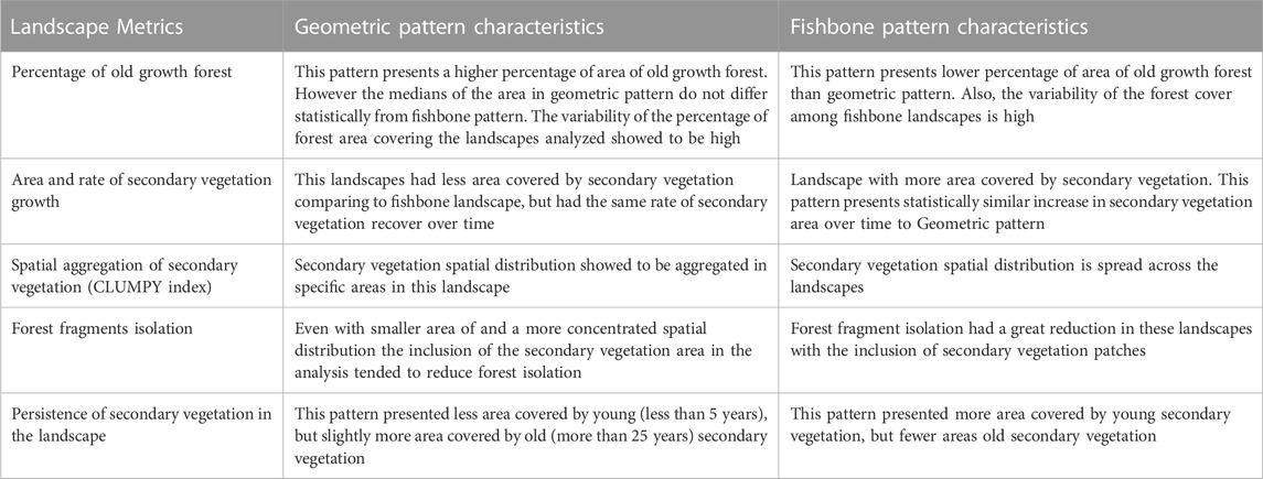
TABLE 1. Summary of landscape characteristics regarding old growth forest and secondary vegetation classes in the two contrasting deforestation patterns in the Amazon: Geometric (n = 7) and Fishbone (n = 7) patterns. Old growth forest and secondary vegetation areas were analyzed every 5 years between 1985 and 2015.
We found a large variation in forest cover for each deforestation pattern across time, even in neighbor landscapes (Figure 2). At the beginning of the study (1985), all landscapes with Geometric and Fishbone patterns had forest cover greater than 80% and no statistical difference in area of mature forest (Mann-Whitney, w = 25, p = 1.00). From 1985, the deforestation process occurred at a different pace, generating landscapes patterns with distinct spatial structures and trajectories. The distinct deforestation and fragmentation trajectories led to landscapes with 17%–70% in Geometric and 18%–62% in Fishbone patterns of forest cover at the end of the period (2015). Although the median forest cover is lower in the Fishbone pattern, we did not find a statistically significant difference in forest cover proportion between patterns at any year during the analysis period (Supplementary Table S1).
3.2 Secondary vegetation trajectories
The area of secondary vegetation in both patterns increased over time (Figure 3 F = 21,835; p = 9,90e-06). The growth rate (i.e., the slope of the line) of secondary vegetation area was similar in both patterns (F = 1.883; p = 0.173), but the Fishbone landscapes had larger areas with secondary vegetation (i.e., the intercept of the line) from the beginning until the end of the time series (F = 18.715; p = 3.78e-05).
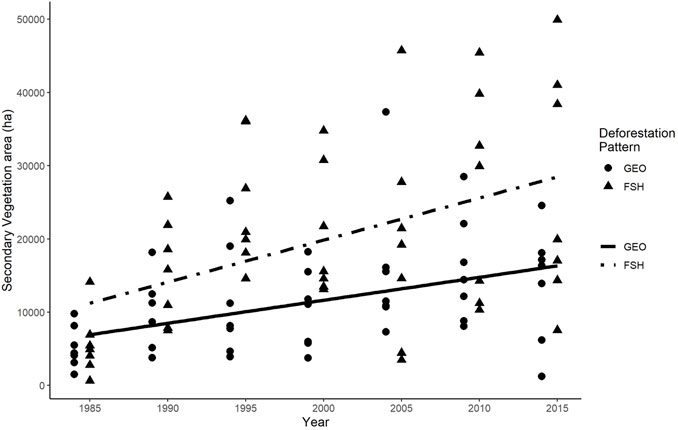
FIGURE 3. Changes in area covered by secondary vegetation over time in Geometric and Fishbone landscapes. The ANCOVA analysis showed no significant difference in the line’s slopes (F = 1.883; p = 0.173), but indicates a significant difference in the magnitude of the secondary vegetation area (F = 18.715; p = 3.78e-05). GEO–Geometric pattern; FSH–Fishbone pattern.
3.3 Spatial configuration of secondary vegetation within landscapes
The aggregation index (CLUMPY) revealed that the secondary vegetation at the Geometric pattern was more aggregated than at the Fishbone pattern. The Mann-Whitney test showed a significant difference between patterns regarding the CLUMPY metric in some years (1990, 2010, and 2015), but not in others (Figure 4). However, there is a clear trend of higher aggregation of secondary vegetation patches within the landscapes with Geometric pattern (see also Supplementary Figure S2). Furthermore, the variability in the Fishbone pattern was higher than in the Geometric pattern in all years of the longitudinal analysis from 1985–2015.
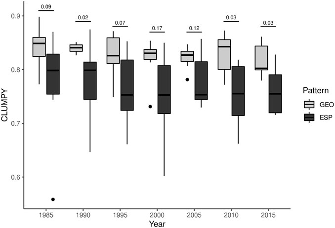
FIGURE 4. Spatial aggregation index of secondary vegetation considering distinct deforestation patterns. CLUMPY–Landscape spatial aggregation metrics. GEO–Geometric pattern of deforestation; FSH–Fishbone pattern of deforestation. The numbers above the graph correspond to the p-value of the Mann-Whitney test.
3.4 The effect of secondary vegetation in reducing old growth forest fragments isolation
The analysis of isolation based on Euclidean Nearest Neighborhood Mean showed that secondary vegetation can reduce forest isolation in both patterns of deforestation (Figure 5). The reduction of forest isolation by the secondary vegetation patches was expressive in both deforestation patterns across all years (Figure 5A; Supplementary Table S3). In landscapes with the Geometric pattern, we found a larger reduction in mean ENN_MN, spanning from 12%–52% while in landscapes with Fishbone pattern, the reduction was found to be between 13% and 27%.
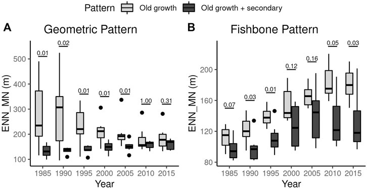
FIGURE 5. Effect of including secondary vegetation on the forest fragments isolation. ENN_MN–Euclidean Nearest Neighborhood Mean. Old growth: Mean isolation of the landscape forest patches considering only the old growth forest fragments. Old growth + secondary: Mean isolation considering both old growth forest and secondary vegetation. (A) Reduction of forest fragment isolation in landscapes with Geometric pattern of deforestation. Great and significant reduction in mean isolation were observed in most of the evaluated years (1985–2005). (B) Reduction of forest fragments isolation in landscapes with Fishbone pattern of deforestation. A significant reduction were only observed in 1990, 1995, and 2015, despite a clear reduction were observed in all years. The numbers above the boxplots correspond to the p-values of Mann-Whitney test.
3.5 Persistence of secondary vegetation in the landscapes
Landscapes with the Fishbone pattern had more secondary vegetation area in initial stages (<5 years old) of regeneration than landscapes with the Geometric pattern (W = 8 and p-value = 0.0378) (Figure 6; Supplementary Table S4). We also found a large variability in Fishbone landscapes at this age category. The GEO pattern had more secondary vegetation of late stages (>25 years old), however this difference was marginally significant (W = 40 and p-value = 0.0530). We did not find statistically significant differences among the other categories of age.
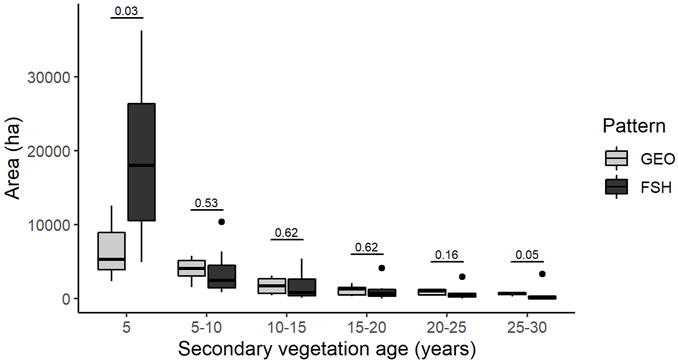
FIGURE 6. Scondary vegetation area on distinct categories of age. GEO–Geometric pattern of deforestation; FSH–Fishbone pattern of deforestation. The numbers above the graph correspond to the p-value of the Mann-Whitney test.
4 Discussion
Our landscape analysis revealed that the Fishbone deforestation pattern, produced by several small household lots, resulted in contexts that allowed a greater forest regeneration, likely due to pasture and agricultural management that frequently uses fallow as part of strategies to recover soil fertility. In this pattern, the secondary vegetation occupied more area and showed to be more spread through the landscape, although tended to be younger. These secondary vegetation characteristics and dynamics, along with the deforestation pattern, likely produce different effects concerning biodiversity and ecosystems conservation.
We found that most of the Fishbone landscapes presented less old growth forest cover, though not statistically different (p > 0.05) than the Geometric landscapes over time (Figure 2). However, we also found a greater variability within groups than between them, which led to non-significative differences when comparing them. This large variability within groups reflects the differences in the occupation process in each region of the Amazon Forest (Machado 1998). The lowest forest cover was found in landscapes located at the state of Rondônia (Southern part of the Amazon’s arc of deforestation) (Supplementary Figure S1). The high number of paved roads plus the proximity of the consuming market of the South and Southeast of Brazil, might explain the intense deforestation activities in this state (Aguiar et al., 2007; Barber et al., 2014). The northern regions, as the landscapes in the states of Roraima and Pará (Figure 1) have highest forest cover. Besides differences in the historical occupational process of the Amazon, there are other factors such as environmental (e.g. rainfall, temperature) (Aide et al., 2013), economic (e.g. financial crisis, tax incentives) (Fearnside 2005; Antonarakis et al., 2022), political and institutional (e.g. mayor or governor reelection, low capacity of enforcement by environmental institutions) (Pailler 2018) that also influence deforestation rates.
We found that both patterns typically gain secondary vegetation area at a similar pace throughout time, but the total amount of secondary vegetation area is greater in the Fishbone landscapes (Figure 3). Therefore, the different processes of land use intensity and landscape management that lead to each deforestation pattern also have long term consequences to natural forest regeneration and landscape structure. In the Geometric pattern, agricultural and livestock practices involve the use of heavy machinery, deforestation and management of the deforested areas, resulting in intense land use, that seeks to maximize production taking advantage of all available land, leaving few abandoned areas (Arima et al., 2015). Conversely, in the Fishbone pattern, it is common that farmers advance to old growth forest, through the slash-and-burn process, for agrarian production and further replacement to extensive cattle ranching (Alencar et al., 2016). Over time, it is common for older pastures in small farming settings to be abandoned and invaded by secondary vegetation due to lack of pasture management, low investment, no technical assistance or no access to machinery (Alves et al., 2003).
Furthermore, we found larger variability in secondary vegetation area in landscapes with Fishbone pattern than with Geometric pattern. This might happen due to Fishbone landscapes having several landowners than in landscapes with Geometric pattern (i.e., several small rural families vs. few large landowners), contributing to variation in land management per landscape (Metzger 2002; Mayer 2019). Farm-level biophysical conditions (e.g., soil type, slope), infrastructure and financial opportunities (e.g., agrarian credit) might be managed differently according to different family strategies (Browder et al., 2004), resulting in more or less intense land management. The secondary vegetation in landscapes with intensive management (i.e., <5 years fallow cycles), for example, might lose its capacity of recovery over time (Jakovac et al., 2015). In addition, proximity to roads and urban areas could also influence natural regeneration rates and total amount of land recovery over time (van Vliet et al., 2012). Alves et al. (2003), for example, showed that rural settlements closer to federal roads have less secondary vegetation than farther settlements. A combination of these effects may explain the variability in secondary vegetation area we found.
Regarding the spatial distribution of the secondary vegetation, some intrinsic characteristics of land use approaches in each deforestation pattern may have influenced their spatial aggregation within landscapes. In the Geometric pattern, it is expected that most areas of secondary vegetation be at the edge of old growth forest fragments and in areas where mechanized agriculture is restricted, such as in terrains with steep slopes (Laue and Arima 2016; Sloan et al., 2016). In the Fishbone landscapes, the growth of secondary vegetation is spread out, since there are more variation in land use between farms (Metzger 2002) and there are more rural properties within the same area (i.e., our 50 × 50 km landscapes), with smaller and more heterogeneous farms than in Geometric landscapes (Arima et al., 2015) (Figure 4). Also, agricultural systems in Fishbone landscapes might be more permissive for natural regeneration since farmers in these landscapes tend to grow crops without heavy machinery (Alves et al., 2003). Small-rural households, such as in INCRA colonization settlements, are more likely to take advantage of forest resources for self-sustaining (e.g., wood, food gathering) (Nunes et al., 2019; Rasmussen et al., 2020), which may encourage these families not to cut the secondary vegetation as soon as it starts to grow. Those characteristics affect in different manners the potential of secondary vegetation to prosper and mitigate the effects of deforestation in each pattern.
Our study also found that secondary vegetation reduces the mean isolation of forest fragments in both patterns of deforestation (Figures 5A, B), but each one has its own dynamics. In Geometric landscapes, the mean isolation of forest fragments decreases over time, even with increase in deforestation (Figure 5A). This effect is more evident in landscapes with few forest fragments, since the complete elimination of small forest fragments decreases the denominator used to calculate the mean isolation of the landscape (Supplementary Figure S1). So, while the landscape is deforested, and the smaller and more isolated forest fragments are eliminated, the mean isolation of the landscape is artificially reduced (Fahrig 2003). When we added the secondary vegetation to the calculation of the metric, we found that the median of the ENN distance distribution increased over time, likely for the same reasons explained above. In Fishbone landscapes, the secondary vegetation also reduced the mean isolation of the forest fragment remnants (Figure 5B). The ENN_MN metric followed the expected behavior: while the total deforestation and forest fragmentation increased, the mean isolation of the landscape also increased.
Another important feature analyzed in this study was the time of persistence of the secondary vegetation in each deforestation pattern. We found that the Fishbone landscapes hold more secondary vegetation up to 5 years old, while the Geometric landscapes had more secondary vegetation of the 25–30 years old category (Figure 6). This unexpected difference can also be related to land use approach present in each deforestation pattern. The most frequent agricultural technique employed in Fishbone areas is the slash-and-burn (Alencar et al., 2016), and it also reuses part of the land after a fallow cycle between periods of cultivation. In the fallow periods, some secondary vegetation grows, but are again slashed and burned after a few years (3–15 years depending on the intensity of land use (Jakovac et al., 2016)). The land use intensification process in riverine communities along Purus River in the state of Amazonas was detected by Jakovac et al. (2016), leading to shorter fallow periods. Perhaps, this intensification may be spreading across the Amazon upland areas (van Vliet et al., 2013; Villa et al., 2018). This detected intensification and the fallow agriculture typical of the Amazon region may explain why most of the secondary vegetation in the Fishbone landscapes seems to not last more than 10 years, and also the surprising amount of secondary vegetation that is less than 5 years old. In Geometric landscapes, as mostly of the land is incorporated into the production system, only the previously deforested, but not suited for large-scale agriculture or pasture plots of land are abandoned. In abandoned areas, secondary vegetation is able to grow and persist for long periods of time (Laue and Arima 2016).
4.1 Implication for biodiversity and ecosystems services
Many studies, also performed in the Amazon Forest, have already investigated the effects of forest loss and forest fragmentation in a variety of animals and plants, (Haddad et al., 2015; Laurance et al., 2018). These studies suggest that given the landscape structure, it is possible to infer several negative and positive impacts of forest loss and fragmentation on local biodiversity and ecosystems services (Fletcher et al., 2018; Fahrig et al., 2019), regarding the limitations that comes with this type of inference (Schindler et al., 2008). In brief, we found that in Geometric landscapes there were few spots of secondary vegetation concentrated in smaller portions of the landscape (Supplementary Figure S1) and they were at more advanced stages of the natural regeneration process (Figure 6). Conversely, in Fishbone landscapes, we found a large number of secondary vegetation patches spread across the landscape and most of them at initial stages of the regeneration (Supplementary Figure S2). These spatial distributions and longitudinal patterns of the secondary vegetation bring different implications to the biodiversity and environmental services provision in each model of land occupation in the Amazon.
The main positive effect of the secondary vegetation to the landscape was its role in the reduction of the mean isolation of forest fragments. This reduction allows landscapes to be more connected, likely improving seed dispersion and mobility of individuals and gene flow of populations throughout the landscape (Dick et al., 2003; Mestre and Gasnier 2008; Bobrowiec and Gribel 2010; Wolfe et al., 2015). Although Fishbone landscapes had less area of mature secondary vegetation, there were more in initial stages spread around the landscape. Small patches of secondary vegetation in initial stages may play an important role in biodiversity conservation for local communities (de Souza et al., 2016). Despite representing few gains in habitat, it increases the connectivity of the landscape and improve the quality of the matrix, which are essential features for a biodiversity-friendly landscape (Melo et al., 2013; Laurance et al., 2018; Arroyo-Rodríguez et al., 2020). For local communities, these secondary vegetation patches might be seen as potential economic resources providing fibers, wood and fruits, complementing their income and daily needs (de Souza et al., 2016; Rasmussen et al., 2020).
Fishbone landscapes had a large recover in habitat amount, however, the value of this vegetation might be limited (Peres et al., 2010), since understory plant and animal species may be unable to colonize these areas properly neither actively use them for food or shelter (Chazdon 2014; Carrara et al., 2015). As most of the secondary vegetation in this landscape is in initial stages of succession, the increase in habitat area might be restricted to a few taxonomic groups (Tabarelli et al., 2012). While in Geometric landscapes, the more persistent areas of secondary vegetation might represent a real gain in habitat, even for the most disturbance-sensitive species. However, the gain of forested land after deforestation is small, representing only 0.95% at the landscapes with higher cover of secondary forest. Generally, landscapes with Geometric pattern should offer less shelter and resources to species that use areas of secondary vegetation, leading to less recovery in landscape connectivity.
The pace of forest recovery in each pattern of deforestation, should also promote different gains in ecosystem services. Fishbone landscapes may be slower in carbon stock recovery over time, since most of the secondary vegetation persisted through less than 5 years (Chazdon 2008). However, these young stands of secondary vegetation can act as strong carbon sinks which brings value for landholders (Naime et al., 2020). Also, as there is more secondary vegetation spread across the landscape, they should promote protection to soil and hydrological resources (Duarte et al., 2016; Strassburg et al., 2016). On the long run, these characteristics might be fundamental to the livelihood maintenance of those rural communities. In the contrary, Geometric landscapes should have less recovery and protection of soil and hydrological resources.
In conclusion, jointly evaluating the studied landscape metrics, there seems to be a distinct pattern of forest natural regeneration for each pattern of deforestation: Geometric and Fishbone. In the landscapes with the Fishbone pattern there is secondary vegetation spread across the landscape. For this reason, we found a larger reduction in old growth forest isolation in Fishbone landscapes than in Geometric landscapes, which have less amount and more aggregated secondary vegetation. These differences are due to the distinct processes of occupation and landscape management over time, reflecting opposite strategies of colonization and occupation in the Amazon Forest. These processes also affected the time of persistence of the secondary vegetation, with the Fishbone pattern having early successional stages while the Geometric pattern showed later stages. The characteristics of secondary vegetation in each deforestation pattern contributes differently to the recovery of biodiversity and ecosystems services. To fully accomplish the recovery of biodiversity and ecosystems services, there must be public policies that stimulates the conservation and the sustainable use of secondary vegetation (e.g., the state of Pará has laws that protect secondary vegetation-(Vieira et al., 2014) without compromising smallholders’ traditional agricultural practices. Those policies should be very clear in the way they define secondary vegetation at the same time they should be flexible enough to accommodate the highly dynamic and uncertain characteristics of a regenerating forest. Despite the importance of national laws to protect secondary vegetation, more localized rules (i.e., state level laws) may have greater success in protecting and ensuring a more sustainable use secondary forest, considering the great variability in area and spatial arrangement of secondary vegetation we found in this study. In addition, further studies that focus on other deforestation patterns (e.g., diffuse, dendritic) should be performed to increase current knowledge about the relationship between deforestation and regeneration patterns in the Amazon. Also, we found large variability in the amount of secondary vegetation within deforestation patterns, thus future studies that seek to explain the regional differences in the patterns of natural regeneration are fundamental to understand the distinct trajectories of forest regeneration in the Amazon Forest.
Furthermore, our results revealed how the type of occupation influences the deforestation pattern, generating landscapes with remarked differences in area, isolation and spatial distribution of forest fragments. In general, the main policies that restrict deforestation inside private properties (e.g., Brazil’s Forest Code (Azevedo et al., 2017); the Cadastro Ambiental Rural—a self-reporting system of land use inside agricultural establishments (Jung et al., 2017)), only consider a area and/or proportion of forest remnants. No criteria is established in these legislation that considers the spatial arrangement of forest remnants, neither within a single property nor considering a group of properties and nearby protected areas.
Although we limited our study to two deforestation patterns in the Amazon, similar patterns were observed in other tropical regions (Mertens and Lambin 1997; Geist and Lambin 2001; Miettinen et al., 2011). According to the literature, these other regions had similar occupation processes, land use types, actors and incentive public policies that resulted in these deforestation patterns (Geist and Lambin 2002). Therefore, it is possible that secondary vegetation regrowth follows the same pattern in other countries as in the Amazon. However, more investigation is needed to verify whether spatial and longitudinal patterns of forest regrowth can be extrapolated to other regions given similar patterns of deforestation. In addition, expanding this analysis for the larger areas, such as the entire Amazon Biome or at national level, would require the use of other image classification techniques, like deep learning algorithms, more suitable for dealing with large volumes of data and temporal series data.
Data availability statement
The datasets presented in this study can be found in online repositories. The names of the repository/repositories and accession number(s) can be found below: https://github.com/alenc09/defpatt_reg.
Author contributions
LA: Conceptualization, data curation, formal analysis, methodology, Writing-Original Draft; ME: conceptualization, methodology, Writing-Review & Editing; JC: conceptualization, Writing-Review & Editing, Supervision.
Acknowledgments
We thank the Biological Dynamics of Forest Fragments Project and the National Institute of Space Research for the structural and logistic support to the execution of this project and to the Coordenação de Aperfeiçoamento de Pessoal de Nível Superior and the Fundação de Amparo à Pesquisa do Estado do Amazonas for the LA’s scholarship (no 024/2014–CAPES/FAPEAM).
Conflict of interest
The authors declare that the research was conducted in the absence of any commercial or financial relationships that could be construed as a potential conflict of interest.
Publisher’s note
All claims expressed in this article are solely those of the authors and do not necessarily represent those of their affiliated organizations, or those of the publisher, the editors and the reviewers. Any product that may be evaluated in this article, or claim that may be made by its manufacturer, is not guaranteed or endorsed by the publisher.
Supplementary material
The Supplementary Material for this article can be found online at: https://www.frontiersin.org/articles/10.3389/fenvs.2023.991695/full#supplementary-material
References
Aguiar, A. P. D., Câmara, G., and Escada, M. I. S. (2007). Spatial statistical analysis of land-use determinants in the Brazilian Amazonia: Exploring intra-regional heterogeneity. Ecol. Model. 209, 169–188. doi:10.1016/j.ecolmodel.2007.06.019
Aide, T. M., Clark, M. L., Grau, H. R., López-Carr, D., Levy, M. A., Redo, D., et al. (2013). Deforestation and reforestation of Latin America and the caribbean (2001-2010). Biotropica 45, 262–271. doi:10.1111/j.1744-7429.2012.00908.x
Alencar, A., Pereira, C., Castro, I., Cardoso, A., Souza, L., Costa, R., et al. (2016). Desmatamento nos Assentamentos da Amazônia: Histórico, tendências e oportunidades. Brasília, DF: Instituto de Pesquisa Ambiental da Amazônia.
Almeida, C. A. de, Coutinho, A. C., Esquerdo, J. C. D. M., Adami, M., Venturieri, A., Diniz, C. G., et al. (2016). High spatial resolution land use and land cover mapping of the Brazilian Legal Amazon in 2008 using Landsat-5/TM and MODIS data. Acta Amaz. 46, 291–302. doi:10.1590/1809-4392201505504
Almeida, C. A., Valeriano, D. M., Escada, M. I. S., and Rennó, C. D. (2010). Estimativa de área de vegetação secundária na Amazônia Legal Brasileira. Acta Amaz. 40, 289–301. doi:10.1590/S0044-59672010000200007
Alves, D. S., Escada, M. I. S., Pereira, J. L. G., and de Albuquerque Linhares, C. (2003). Land use intensification and abandonment in Rondônia, Brazilian Amazônia. Int. J. Remote Sens. 24, 899–903. doi:10.1080/0143116021000015807
Alves, M. T. R., Piontekowski, V. J., Buscardo, E., Pedlowski, M. A., Sano, E. E., and Matricardi, E. A. T. (2021). Effects of settlement designs on deforestation and fragmentation in the Brazilian Amazon. Land Use Policy 109, 105710. doi:10.1016/j.landusepol.2021.105710
Antonarakis, A. S., Pacca, L., and Antoniades, A. (2022). The effect of financial crises on deforestation: A global and regional panel data analysis. Sustain Sci. 17, 1037–1057. doi:10.1007/s11625-021-01086-8
Arima, E. Y., Walker, R. T., Perz, S., and Souza, C. (2015). Explaining the fragmentation in the Brazilian Amazonian forest. J. Land Use Sci. 2015, 1–21. doi:10.1080/1747423X.2015.1027797
Arroyo-Rodríguez, V., Fahrig, L., Tabarelli, M., Watling, J. I., Tischendorf, L., Benchimol, M., et al. (2020). Designing optimal human-modified landscapes for forest biodiversity conservation. Ecol. Lett. 23, 1404–1420. doi:10.1111/ele.13535
Arroyo-Rodríguez, V., Melo, F. P. L., Martínez-Ramos, M., Bongers, F., Chazdon, R. L., Meave, J. A., et al. (2017). Multiple successional pathways in human-modified tropical landscapes: New insights from forest succession, forest fragmentation and landscape ecology research. Biol. Rev. 92, 326–340. doi:10.1111/brv.12231
Auffret, A. G., Rico, Y., Bullock, J. M., Hooftman, D. A. P., Pakeman, R. J., Soons, M. B., et al. (2017). Plant functional connectivity - integrating landscape structure and effective dispersal. J. Ecol. 105, 1648–1656. doi:10.1111/1365-2745.12742
Azevedo, A. A., Rajão, R., Costa, M. A., Stabile, M. C. C., Macedo, M. N., dos Reis, T. N. P., et al. (2017). Limits of Brazil's Forest Code as a means to end illegal deforestation. Proc. Natl. Acad. Sci. U.S.A. 114, 7653–7658. doi:10.1073/pnas.1604768114
Barber, C. P., Cochrane, M. A., Souza, C. M., and Laurance, W. F. (2014). Roads, deforestation, and the mitigating effect of protected areas in the Amazon. Biol. Conserv. 177, 203–209. doi:10.1016/j.biocon.2014.07.004
Bins, L. S., Erthal, G. J., and Fonseca, L. M. G. (1993). Um método de Classificação Não Supervisionada por Regiões. SIBGRAPI VI 1993, 65–68.
Bobrowiec, P. E. D., and Gribel, R. (2010). Effects of different secondary vegetation types on bat community composition in Central Amazonia, Brazil. Anim. Conserv. 13, 204–216. doi:10.1111/j.1469-1795.2009.00322.x
Browder, J. O., Pedlowski, M. A., and Summers, P. M. (2004). Land use patterns in the Brazilian Amazon: Comparative farm-level evidence from Rondônia. Hum. Ecol. 32, 197–224. doi:10.1023/B:HUEC.0000019763.73998.c9
Câmara, G., Souza, R. C. M., Freitas, U. M., and Garrido, J. (1996). Spring: Integrating remote sensing and gis by object-oriented data modelling. Comput. Graph 20, 395–403. doi:10.1016/0097-8493(96)00008-8
Carrara, E., Arroyo-Rodríguez, V., Vega-Rivera, J. H., Schondube, J. E., de Freitas, S. M., and Fahrig, L. (2015). Impact of landscape composition and configuration on forest specialist and generalist bird species in the fragmented Lacandona rainforest, Mexico. Biol. Conserv. 184, 117–126. doi:10.1016/j.biocon.2015.01.014
Chase, J. M., Jeliazkov, A., Ladouceur, E., and Viana, D. S. (2020). Biodiversity conservation through the lens of metacommunity ecology. Ann. N.Y. Acad. Sci. 1469, 86–104. doi:10.1111/nyas.14378
Chazdon, R. (2012) Regeneração de florestas tropicais Tropical forest regeneration. Bol. do Mus. Para. Emílio Goeldi. Ciências Nat. 7:24. doi:10.46357/bcnaturais.v7i3.587
Chazdon, R. (2014). Second growth: The promise of tropical forest regeneration in an age of defor-estation. 1st edn Chicago: The University of chicago Press.
Chazdon, R. L. (2008). Beyond deforestation: Restoring forests and ecosystem services on degraded lands. Science 320, 1458–1460. doi:10.1126/science.1155365
De Faria, B. L., Marano, G., Piponiot, C., Silva, C. A., Dantas, V. d. L., Rattis, L., et al. (2020). Model-based estimation of amazonian forests recovery time after drought and fire events. Forests 12, 8. doi:10.3390/f12010008
de Filho, F. J. B., and Metzger, J. P. (2006). Thresholds in landscape structure for three common deforestation patterns in the Brazilian Amazon. Landsc. Ecol. 21, 1061–1073. doi:10.1007/s10980-006-6913-0
de Souza, S. E. X. F., Vidal, E., Chagas, G. de F., Elgar, A. T., and Brancalion, P. H. S. (2016). Ecological outcomes and livelihood benefits of community-managed agroforests and second growth forests in Southeast Brazil. Biotropica 48, 868–881. doi:10.1111/btp.12388
Dick, C. W., Etchelecu, G., and Austerlitz, F. (2003). Pollen dispersal of tropical trees (Dinizia excelsa: Fabaceae) by native insects and African honeybees in pristine and fragmented Amazonian rainforest. Mol. Ecol. 12, 753–764. doi:10.1046/j.1365-294X.2003.01760.x
dos Santos Silva, M. P. dos S., Câmara, G., Escada, M. I. S., and de Souza, R. C. M. de (2008). Remote-sensing image mining: Detecting agents of land-use change in tropical forest areas. Int. J. Remote Sens. 29, 4803–4822. doi:10.1080/01431160801950634
Eycott, G. T., Stewart, M. C., Buyung-Ali, A. P., Bowler, D. E., Watts, K., and Pullin, A. S. (2012). A meta-analysis on the impact of different matrix structures on species movement rates. Landsc. Ecol. 27, 1263–1278. doi:10.1007/s10980-012-9781-9
Fahrig, L., Arroyo-Rodríguez, V., Bennett, J. R., Boucher-Lalonde, V., Cazetta, E., Currie, D. J., et al. (2019). Is habitat fragmentation bad for biodiversity? Biol. Conserv. 230, 179–186. doi:10.1016/j.biocon.2018.12.026
Fahrig, L. (2003). Effects of habitat fragmentation on biodiversity. Annu. Rev. Ecol. Evol. Syst. 34, 487–515. doi:10.1146/annurev.ecolsys.34.011802.132419
Fearnside, P. M. (2005). Deforestation in Brazilian Amazonia: History, rates, and consequences. Conserv. Biol. 19, 680–688. doi:10.1111/j.1523-1739.2005.00697.x
Fletcher, R. J., Didham, R. K., Banks-Leite, C., Barlow, J., Ewers, R. M., Rosindell, J., et al. (2018). Is habitat fragmentation good for biodiversity? Biol. Conserv. 226, 9–15. doi:10.1016/j.biocon.2018.07.022
Geist, H., and Lambin, E. (2001). What drives tropical deforestation? Louvain-la-Neuve: LUCC International Project Office.
Geist, H. J., and Lambin, E. F. (2002). Proximate causes and underlying driving forces of tropical deforestation. BioScience 52, 143. doi:10.1641/0006-3568(2002)052[0143:pcaudf]2.0.co;2
Haddad, N. M., Brudvig, L. A., Clobert, J., Davies, K. F., Gonzalez, A., Holt, R. D., et al. (2015). Habitat fragmentation and its lasting impact on Earth's ecosystems. Sci. Adv. 1, e1500052. doi:10.1126/sciadv.1500052
Hall, J. S., Plisinski, J. S., Mladinich, S. K., van Breugel, M., Lai, H. R., Asner, G. P., et al. (2022). Deforestation scenarios show the importance of secondary forest for meeting Panama's carbon goals. Landsc. Ecol. 37, 673–694. doi:10.1007/s10980-021-01379-4
Hart, A. (2001). Mann-whitney test is not just a test of medians: Differences in spread can be important. BMJ 323, 391–393. doi:10.1136/bmj.323.7309.391
Hoelle, J. (2014). Cattle culture in the Brazilian Amazon. Hum. Organ. 73, 363–374. doi:10.17730/humo.73.4.u61u675428341165
Jakovac, C. C., Peña-Claros, M., Kuyper, T. W., and Bongers, F. (2015). Loss of secondary-forest resilience by land-use intensification in the Amazon. J. Ecol. 103, 67–77. doi:10.1111/1365-2745.12298
Jakovac, C. C., Peña-Claros, M., Mesquita, R. C. G., Bongers, F., and Kuyper, T. W. (2016). Swiddens under transition: Consequences of agricultural intensification in the Amazon. Agric. Ecosyst. Environ. 218, 116–125. doi:10.1016/j.agee.2015.11.013
Jones, I. L., DeWalt, S. J., Lopez, O. R., Bunnefeld, L., Pattison, Z., and Dent, D. H. (2019). Above- and belowground carbon stocks are decoupled in secondary tropical forests and are positively related to forest age and soil nutrients respectively. Sci. Total Environ. 697, 133987. doi:10.1016/j.scitotenv.2019.133987
Jung, S., Rasmussen, L. V., Watkins, C., Newton, P., and Agrawal, A. (2017). Brazil's national environmental registry of rural properties: Implications for livelihoods. Ecol. Econ. 136, 53–61. doi:10.1016/j.ecolecon.2017.02.004
Laue, J. E., and Arima, E. Y. (2016). Spatially explicit models of land abandonment in the Amazon. J. Land Use Sci. 11, 48–75. doi:10.1080/1747423X.2014.993341
Laurance, W. F., Camargo, J. L. C., Fearnside, P. M., Lovejoy, T. E., Williamson, G. B., Mesquita, R. C. G., et al. (2018). AnAmazonian rainforest and its fragments as a laboratory of global change. Biol. Rev. 93, 223–247. doi:10.1111/brv.12343
Lee, R. H., Morgan, B., Liu, C., Fellowes, J. R., and Guénard, B. (2021). Secondary forest succession buffers extreme temperature impacts on subtropical Asian ants. Ecol. Monogr. 91, e01480. doi:10.1002/ecm.1480
Machado, L. (1998). “A fronteira agrígola na Amazônia brasileira,” in Geografia e Meio Ambiente no BrasilApropriação e uso do território Brasileiro.pdf. 2nd edn. (São Paulo: Hucite).
MapBiomas (2022) Projeto MapBiomas – coleção 5.0 da Série Anual de Mapas de Cobertura e Uso de Solo do Brasil. Available at: https://plataforma.brasil.mapbiomas.org. [Accessed 2 Feb 2022].
Mayer, A. L. (2019). Family forest owners and landscape-scale interactions: A review. Landsc. Urban Plan. 188, 4–18. doi:10.1016/j.landurbplan.2018.10.017
Melo, F. P. L., Arroyo-Rodríguez, V., Fahrig, L., Martínez-Ramos, M., and Tabarelli, M. (2013). On the hope for biodiversity-friendly tropical landscapes. Trends Ecol. Evol. 28, 462–468. doi:10.1016/j.tree.2013.01.001
Mertens, B., and Lambin, E. (1999). Modelling land cover dynamics: Integration of fine-scale land cover data with landscape attributes. Int. J. Appl. Earth Observation Geoinformation 1, 48–52. doi:10.1016/S0303-2434(99)85027-2
Mertens, B., and Lambin, E. F. (1997). Spatial modelling of deforestation in southern Cameroon. Appl. Geogr. 17, 143–162. doi:10.1016/S0143-6228(97)00032-5
Mesquita, R. de C. G., Massocados, P. E. S., Jakovac, C. C., Bentos, T. V., and Williamson, G. B. (2015). Amazon rain forest succession: Stochasticity or land-use legacy? BioScience 65, 849–861. doi:10.1093/biosci/biv108
Mestre, L. A. M., and Gasnier, T. R. (2008). Populates de aranhas errantes do genero Ctenus em fragmentos florestais na Amazonia Central. SciELO 38, 6. doi:10.1590/s0044-59672008000100018
Metzger, J. P. (2002). Landscape dynamics and equilibrium in areas of slash-and-burn agriculture with short and long fallow period (Bragantina region, NE Brazilian Amazon). Landsc. Ecol. 17, 419–431. doi:10.1023/a:1021250306481
Miettinen, J., Shi, C., and Liew, S. C. (2011). Deforestation rates in insular Southeast asia between 2000 and 2010. Glob. Change Biol. 17, 2261–2270. doi:10.1111/j.1365-2486.2011.02398.x
Molin, P. G., Chazdon, R., Frosini de Barros Ferraz, S., and Brancalion, P. H. S. (2018). A landscape approach for cost-effective large-scale forest restoration. J. Appl. Ecol. 55, 2767–2778. doi:10.1111/1365-2664.13263
Naime, J., Mora, F., Sánchez-Martínez, M., Arreola, F., and Balvanera, P. (2020). Economic valuation of ecosystem services from secondary tropical forests: Trade-offs and implications for policy making. For. Ecol. Manag. 473, 118294. doi:10.1016/j.foreco.2020.118294
Nunes, A. V., Peres, C. A., Constantino, P. de A. L., Santos, B. A., and Fischer, E. (2019). Irreplaceable socioeconomic value of wild meat extraction to local food security in rural Amazonia. Biol. Conserv. 236, 171–179. doi:10.1016/j.biocon.2019.05.010
Pailler, S. (2018). Re-election incentives and deforestation cycles in the Brazilian Amazon. J. Environ. Econ. Manag. 88, 345–365. doi:10.1016/j.jeem.2018.01.008
Peres, C. A., Gardner, T. A., Barlow, J., Zuanon, J., Michalski, F., Lees, A. C., et al. (2010). Biodiversity conservation in human-modified Amazonian forest landscapes. Biol. Conserv. 143, 2314–2327. doi:10.1016/j.biocon.2010.01.021
Poorter, L., Craven, D., Jakovac, C. C., van der Sande, M. T., Amissah, L., Bongers, F., et al. (2021). Multidimensional tropical forest recovery. Science 374, 1370–1376. doi:10.1126/science.abh3629
Prist, P. R., Michalski, F., and Metzger, J. P. (2012). How deforestation pattern in the Amazon influences vertebrate richness and community composition. Landsc. Ecol. 27, 799–812. doi:10.1007/s10980-012-9729-0
Rasmussen, L. V., Fagan, M. E., Ickowitz, A., Wood, S. L. R., Kennedy, G., Powell, B., et al. (2020). Forest pattern, not just amount, influences dietary quality in five African countries. Glob. Food Secur. 25, 100331. doi:10.1016/j.gfs.2019.100331
Ribeiro, S. E., de Almeida-Rocha, J. M., Weber, M. M., Kajin, M., Lorini, M. L., and Cerqueira, R. (2021). Do anthropogenic matrix and life-history traits structure small mammal populations? A meta-analytical approach. Conserv. Genet. 22, 703–716. doi:10.1007/s10592-021-01352-3
Rocha, G. P. E., Vieira, D. L. M., and Simon, M. F. (2016). Fast natural regeneration in abandoned pastures in southern Amazonia. For. Ecol. Manag. 370, 93–101. doi:10.1016/j.foreco.2016.03.057
Rosa, I. M. D., Gabriel, C., and Carreiras, J. M. B. (2017). Spatial and temporal dimensions of landscape fragmentation across the Brazilian Amazon. Reg. Environ. Change 17, 1687–1699. doi:10.1007/s10113-017-1120-x
Saito, É. A., Fonseca, L. M. G., Escada, M. I. S., and Korting, T. S. (2011). Efeitos da mudança de escala em padrões de desmatamento na Amazônia. Rev. Bras. Cartogr. 63, 14.
San-José, M., Arroyo-Rodríguez, V., and Meave, J. A. (2020). Regional context and dispersal mode drive the impact of landscape structure on seed dispersal. Ecol. Appl. 30. doi:10.1002/eap.2033
Schindler, S., Poirazidis, K., and Wrbka, T. (2008). Towards a core set of landscape metrics for biodiversity assessments: A case study from dadia national park, Greece. Ecol. Indic. 8, 502–514. doi:10.1016/j.ecolind.2007.06.001
Shimabukuro, Y. E., and Smith, J. A. (1991). The least-squares mixing models to generate fraction images derived from remote sensing multispectral data. IEEE Trans. Geosci. Remote Sens. 29, 16–20. doi:10.1109/36.103288
Silva Junior, C. H. L., Heinrich, V. H. A., Freire, A. T. G., Broggio, I. S., Rosan, T. M., Doblas, J., et al. (2020). Benchmark maps of 33 years of secondary forest age for Brazil. Sci. Data 7, 269. doi:10.1038/s41597-020-00600-4
Sloan, S., Goosem, M., and Laurance, S. G. (2016). Tropical forest regeneration following land abandonment is driven by primary rainforest distribution in an old pastoral region. Landsc. Ecol. 31, 601–618. doi:10.1007/s10980-015-0267-4
Strassburg, B. B. N., Barros, F. S. M., Crouzeilles, R., Iribarrem, A., Santos, J. S. d., Silva, D., et al. (2016). The role of natural regeneration to ecosystem services provision and habitat availability: A case study in the Brazilian atlantic forest. Biotropica 48, 890–899. doi:10.1111/btp.12393
Tabarelli, M., Peres, C. A., and Melo, F. P. L. (2012). The 'few winners and many losers' paradigm revisited: Emerging prospects for tropical forest biodiversity. Biol. Conserv. 155, 136–140. doi:10.1016/j.biocon.2012.06.020
United States Geological Survey (USGS) (2019). Earth explorer. Available at: https://earthexplorer.usgs.gov/ (Accessed March 1, 2017).
van Meerveld, H. J., Jones, J. P. G., Ghimire, C. P., Zwartendijk, B. W., Lahitiana, J., Ravelona, M., et al. (2021). Forest regeneration can positively contribute to local hydrological ecosystem services: Implications for forest landscape restoration. J. Appl. Ecol. 58, 755–765. doi:10.1111/1365-2664.13836
van Vliet, N., Adams, C., Vieira, I. C. G., and Mertz, O. (2013). "Slash and burn" and "shifting" cultivation systems in forest agriculture frontiers from the Brazilian Amazon. Soc. Nat. Resour. 26, 1454–1467. doi:10.1080/08941920.2013.820813
van Vliet, N., Mertz, O., Heinimann, A., Langanke, T., Pascual, U., Schmook, B., et al. (2012). Trends, drivers and impacts of changes in swidden cultivation in tropical forest-agriculture frontiers: A global assessment. Glob. Environ. Change 22, 418–429. doi:10.1016/j.gloenvcha.2011.10.009
Vieira, I., Gardner, T., Ferreira, J., Lees, A., and Barlow, J. (2014). Challenges of governing second-growth forests: A case study from the Brazilian amazonian state of Pará. Forests 5, 1737–1752. doi:10.3390/f5071737
Villa, P. M., Martins, S. V., de Oliveira Neto, S. N., Rodrigues, A. C., Martorano, L. G., Monsanto, L. D., et al. (2018). Intensification of shifting cultivation reduces forest resilience in the northern Amazon. For. Ecol. Manag. 430, 312–320. doi:10.1016/j.foreco.2018.08.014
Wang, X., Blanchet, F. G., and Koper, N. (2014). Measuring habitat fragmentation: An evaluation of landscape pattern metrics. Methods Ecol. Evol. 5, 634–646. doi:10.1111/2041-210X.12198
Watling, J. I., Nowakowski, A. J., Donnelly, M. A., and Orrock, J. L. (2011). Meta-analysis reveals the importance of matrix composition for animals in fragmented habitat. Glob. Ecol. Biogeogr. 20, 209–217. doi:10.1111/j.1466-8238.2010.00586.x
Keywords: forest fragmentation, natural regeneration, remote sensing, landscape metrics, ANCOVA
Citation: Alencar L, Escada MIS and Camargo JLC (2023) Forest regeneration pathways in contrasting deforestation patterns of Amazonia. Front. Environ. Sci. 11:991695. doi: 10.3389/fenvs.2023.991695
Received: 11 July 2022; Accepted: 17 January 2023;
Published: 30 January 2023.
Edited by:
Marco Girardello, University of the Azores, PortugalReviewed by:
Siqi Lu, University of Connecticut, United StatesDaliana Lobo Torres, Pontifical Catholic University of Rio de Janeiro, Brazil
Copyright © 2023 Alencar, Escada and Camargo. This is an open-access article distributed under the terms of the Creative Commons Attribution License (CC BY). The use, distribution or reproduction in other forums is permitted, provided the original author(s) and the copyright owner(s) are credited and that the original publication in this journal is cited, in accordance with accepted academic practice. No use, distribution or reproduction is permitted which does not comply with these terms.
*Correspondence: Lucas Alencar, YWxlbmNhci5sdWNhc2NAZ21haWwuY29t