Research on the fugitive soil dust emission inventory in Western China based on wind erosion equation parameter optimization

The Wind Erosion Equation, currently one of the primary methods for estimating fugitive soil dust emission inventory, is influenced by several factors. Taking the convergent areas of the Tibet Plateau, Loess Plateau, and Qinba Mountains in Western China, we have optimized the climate factor using the WRF model driven by ERA5 reanalysis data. Additionally, we have modified the vegetation cover factors via normalized difference vegetation index and considered the impacts of the land use and cover change. Subsequently, other factors were allocated utilizing geographic information system, and the grid-based fugitive soil dust emission inventory for the study area for 2019 was derived through calculation. Based on the climate factor and vegetation cover factor, we have come up with the monthly allocation coefficients. The study has revealed the following findings: (1) Climate factors are unevenly distributed throughout the focused region, with the Loess Plateau showing the highest value, followed by the Tibet Plateau and the Qinba Mountains. There are also significant variations in the distribution of these factors among municipalities and counties; (2) The order of vegetation cover factor, primarily influenced by regional background as well as agricultural and pastoral activities, in the Loess Plateau, Tibetan Plateau and Qinba Mountains, is consistent with that of the wind erosion index; (3) In 2019, fugitive dust emissions from total suspended particles, PM₁₀, and PM_2.5 reached 9835.9, 2950.8, and 491.8 kt/a, respectively. The Loess Plateau exhibited the highest emission intensity due to factors such as low vegetation coverage, precipitation, high wind speed and wind erosion index; (4) Climate factor and vegetation cover factor are the primary factors influencing the monthly allocation coefficients. In 2019, the highest monthly fugitive dust emissions were estimated in April, accounting for approximately 36.21% of the total. The second and third-highest were found in August and June, respectively. This phenomenon can be explained climatically, as the Loess Plateau, semi-arid and arid regions, did not experience a significant increase in rainfall corresponding to rising temperatures.

1 Introduction

Particulate matter (PM) in the atmosphere has detrimental effects on both human health and atmospheric visibility, with a particular concern for PM_2.5 (Apte et al., 2015; Liu et al., 2016; Ji et al., 2020). To address these challenges, China introduced the “Air Pollution Prevention and Control Action Plan” (The State Council, 2013) in 2013 and the “Three-Year Action Plan to Fight Air Pollution” (The State Council, 2018) in 2018. These plans aim to achieve targeted pollution control through pollution source inventories, numerical modeling, and receptor models, to continuously address PM₁₀ and PM_2.5 pollution and improve urban air quality (Wang et al., 2014; Cheng et al., 2017; Zhang et al., 2017; Shang et al., 2018; Asian Clean Air Center, 2021). However, compiling emission inventories for certain atmospheric pollution sources in complex terrains still presents challenges, such as the fugitive soil dust (FSD) emission inventory. FSD refers to the PM generated directly from exposed surfaces, including agricultural fields, bare mountains, mudflats/tidal flats, dried river valleys, and undeveloped or unvegetated lands, due to natural forces such as wind erosion or anthropogenic activities (Ministry of Environmental Protection, 2014). FSD represents a major source of PM in the ambient air, particularly in the arid and semi-arid regions of Northwestern China (Song et al., 2016).

Wind erosion, categorized as soil erosion, involves the displacement of soil particles under the influence of certain wind forces, including migration, creeping, and suspension. It primarily encompasses fine dust in the form of aerosols, sand drifting, and coarse particles displacing on the ground (Zhang et al., 2002). The results of receptor models indicate that fugitive dust is responsible for 10%–24% of ambient PM₁₀ in cities such as Urumqi, Taiyuan, Anyang, Tianjin, and Jinan. (Bi et al., 2007). However, due to the uncertainties associated with FSD emission inventory compilation, several regional emission inventory studies currently exclude FSD (Zheng et al., 2009; Fu et al., 2013; Qi et al., 2017; Liu H. et al., 2018).

In the 1960s, Woodruff and Siddoway, (1965) and the U.S. Department of Agriculture conduced extensive research on wind erosion in farmlands, leading to development of the Wind Erosion Equation (WEQ). This empirical model established relationships between wind erosion rates and various influencing factors (Skidmore and Woodruff, 1968). Subsequently, as the understanding of wind erosion mechanisms improved, several other models were subsequently developed, including the Revised Wind Erosion Equation (Fryrear et al., 2000), the Texas Erosion Analysis Model (Gregory et al., 2004), the Wind Erosion Assessment Model (Shao et al., 1996), and the Wind Erosion Prediction System (Buschiazzo and Zobeck, 2008). Although these later models offer more refined and accurate predictions compared with WEQ (Buschiazzo and Zobeck, 2008; Zou et al., 2014; Liu et al., 2021), they require more detailed input parameters and involve higher technical complexity, making them unsuitable for large-scale regional FSD emission inventory compilation. In contrast, the WEQ is widely adopted due to its simplicity, operational feasibility, and ease of implementation (Xuan et al., 2000; Panebianco and Buschiazzo, 2008; Mandakh et al., 2016; Xu et al., 2016; Liu A. B. et al., 2018). The WEQ has been endorsed by the United States Environmental Protection Agency (Cowherd et al., 1974; Jutze and Axetell, 1974) and the California Air Resources Board (Countess Environmental, 2006). In 2014, the Ministry of Ecology and Environment of the People’s Republic of China officially designated the WEQ model as the recommended calculation method for FSD emission inventory compilation (Ministry of Environmental Protection, 2014).

Some researchers have utilized the WEQ and incorporated normalized difference vegetation index (NDVI) data for estimating vegetation cover and urban meteorological data for calculating regional climate factor to compute FSD emission inventory for the Beijing–Tianjin–Hebei region and the 2 + 26 cities across China (Li et al., 2020; Li et al., 2021; Song et al., 2021). However, in complex terrains, meteorological factors observed at national basic and general meteorological stations cannot fully represent the distribution of meteorological factors in administrative regions such as cities, counties, or districts, due to the influence of atmospheric circulation, topography, latitude, solar radiation, and water vapor conditions. Consequently, the climate factor required for WEQ calculations, such as annual mean wind speed, monthly precipitation, and monthly mean temperature, exhibit heterogeneity within the same city, county, or district.

To address these limitations, we propose a method in this study to further optimize the WEQ’s parameter and develop a high spatiotemporal-resolution FSD emission inventory. Our approach improves the accuracy of WRF simulations using the ECMWF-ERA5 climate reanalysis dataset and calculates the climate factor of WEQ based on the WRF simulation results. This approach reduces the errors in calculating climate factor within the WEQ model caused by the uniform adoption of meteorological data from city, county, or district meteorological stations. According to the land use and cover change (LUCC) data, adjustments are made to the vegetation cover factor for grids representing construction land, paddy fields, water area, and areas with high vegetation coverage. Furthermore, monthly allocation coefficients are proposed based on the estimated annual mean fugitive soil dust emissions. We apply this methodology to estimate the FSD emission inventory in the convergence areas of the Tibet Plateau, Loess Plateau, and Qinba Mountains in Western China, and investigate the variations among different contributing factors.

2 Data and methods

2.1 Study area

The study area encompasses the eastern part of the Tibet Plateau, the southwestern part of the Loess Plateau, and the northwestern part of the Qinba Mountains in Western China. It includes several prefecture-level regions across different provinces. In Gansu Province, the cities of Tianshui, Longnan, Pingliang, Qingyang, Baiyin, Lanzhou, Linxia, Gannan, and Wuwei are within the study area. Qinghai Province is represented by Xining city, Haidong, Huangnan, and Hainan prefecture. The Shaanxi Province includes Xi’an, Xianyang, Yulin, Weinan, Hanzhong, Yan’an, Tongchuan, Shangluo, and Ankang cities. Zhongwei, Guyuan, and Wuzhong cities fall within the study area of Ningxia Autonomous Region. Lastly, Sichuan Province encompasses Guangyuan, Mianyang, Bazhong cities, and Aba prefecture. The study area displays diverse topography, with the western region dominated by the Tibet Plateau, characterized by high-altitude terrain. In the northern and northeastern parts, the prominent feature is the Loess Plateau, characterized by relatively higher elevations and a network of gullies. The southern region is primarily occupied by the Qinba Mountains, featuring lower elevations but more intricate terrain compared to the Loess Plateau, as illustrated in Figure 1.

FIGURE 1

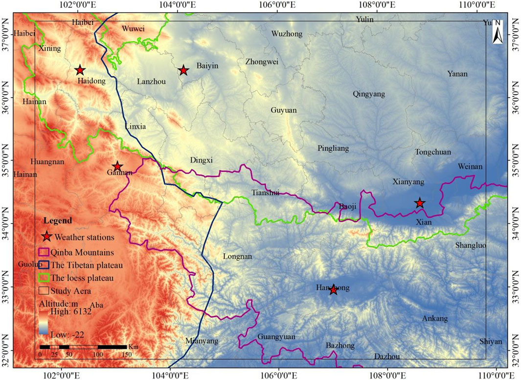
FIGURE 1. Geographical elevation and weather stations of the study area in Western China.

2.2 Introduction to the WEQ

The estimation model adopted in this paper is WEQ, which is represented as follows:

$\mathrm{W}=\text{EF}\times \mathrm{A}(2.1)$

$\text{EF}=\mathrm{\alpha }\times \mathrm{k}\times \mathrm{I}\times \mathrm{K}\times \mathrm{C}\times \mathrm{L}\times \mathrm{V}(2.2)$

Where W represents the FSD emission, and EF denotes the annual emission intensity factor for wind-eroded FSD, measured in t·(hm²·a)⁻¹. A corresponds to the area of the study area (unit: hm²). α is the dimensionless proportion coefficient of total suspended particles (TSP) to the total loss induced by wind erosion, with a reference value of 2.5% recommended by the United States Environmental Protection Agency (USEPA). In this model, k represents the PM percentage in FSD and it is dimensionless whereas TSP, PM₁₀, PM_2.5 are set to be 1.0, 0.3, and 0.05, respectively. (Chepil, 1958; Craig and Turelle, 1964; Jutze and Axetell, 1976). I represents the wind erosion index, measured in t·(hm²·a)⁻¹; K represents the surface roughness factor (dimensionless); C represents the climate factor (dimensionless), as presented in Eqs 2.3, 2.4 respectively; L represents the unshielded width factor (dimensionless). V represents the vegetation cover factor, which indicates the proportion of bare soil area to the total calculated area and is dimensionless (Jutze and Axetell, 1976; US. Environmental Protection Agency, 1977; Skidmore, 1986), as shown in Eq. 2.5.

$C=3.86\times u^3/{\left(PE\right)}^2(2.3)$

$\text{PE}=3.16\times {\displaystyle \sum _{i=1}^{12}}\left[\frac{Pi}{\left(1.8Ti+22\right)}\right.{]}^{10/9}(2.4)$

$\mathrm{V}=1-\text{VC}(2.5)$

Where, u represents the annual mean wind speed, corresponding to the annual mean 10-m wind speed in meteorology, (unit:m·s^-1). PE represents the Thornthwaite’s precipitation–evapotranspiration index (dimensionless), calculated using Eq. 2.4. P_i denotes the monthly precipitation in month i (unit: mm), with a minimum value of 12.7 mm for P_i < 12.7 mm. T_i stands for the monthly mean temperature measured in °C, corresponding to monthly mean ground temperature in meteorology, with a minimum value of −1.7°C for Ti < −1.7°C (Lyles, 1983; Panebianco and Buschiazzo, 2008). VC refers to the proportion of the area covered by the vertical projection per unit area of the vegetation and is dimensionless (Gitelson et al., 2002). VC was calculated using the binary pixel model (Jia et al., 2013), as shown in Eq. 2.6.

$\text{VC}=\left(\text{NDVI}-{\text{NDVI}}_{\text{soil}}\right)/\left({\text{NDVI}}_{\text{veg}}-{\text{NDVI}}_{\text{soil}}\right)(2.6)$

Where, VC represents the vegetation cover of the pixel, where NDVI and NDVI_soil denote the NDVI values of the pixel and non-vegetated land, respectively, with the latter being the minimum NDVI value. NDVI_veg is the NDVI value of vegetated land, which can be considered as the maximum NDVI value. In this study, the upper and lower thresholds of NDVI were defined to represent NDVI_soil and NDVI_veg, respectively, at a 5% confidence level.

2.3 Data sources and processing methods

ERA5 is the fifth generation European Centre for Medium-Range Weather Forecasts (ECMWF) atmospheric reanalysis of the global climate. The ECMWF-ERA5 reanalysis dataset has a horizontal grid resolution of 0.25 × 0.25 and comprises 137 pressure levels in the vertical direction, with a temporal resolution of 1 h. In this study, the ECMWF-ERA5 dataset is used to provide initial boundary conditions for the WRF model simulations. Surface observation data of the stations in Baiyin (Baiyin station), Haidong (Ping’an station), Gannan (Hezuo station), Xianyang (Qindu station), and Hanzhong (Hanzhong station) for the year 2019 were obtained from the CMA Meteorological Data Centre (http://data.cma.cn/data/detail/dataCode/A.0012.0001.html), as presented in Figure 1. To quantitatively analyze the performance of the WRF model simulation, the model results will be assessed by using four commonly used statistical metrics, namely, the correlation coefficient (R), root mean square error (RMSE), mean fractional bias (MFB), and mean fractional error (MFE) (Taylor, 2001).

$\mathrm{R}=\frac{{\sum }_{i=1}^N\left(P_i-\overline{P}\right)\left(O_i-\overline{O}\right)}{\sqrt{{\sum }_{i=1}^N{\left(P_i-\overline{P}\right)}^2}\times \sqrt{{\sum }_{i=1}^N{\left(O_i-\overline{O}\right)}^2}}(2.7)$

$\text{RMSE}=\sqrt{\frac{1}{N}{\sum }_{i=1}^N{\left(P_i-O_i\right)}^2}(2.8)$

$MFB=\frac{1}{N}{\sum }_i^N\frac{P_i-O_i}{O_i+P_i/2}(2.9)$

$MFE=\frac{1}{N}{\sum }_i^N\frac{\left|P_i-O_i\right|}{O_i+P_i/2}(2.10)$

Where, P_i and O_i represent the simulated and observed data, respectively, N denotes the number of samples, and $\overline{P}$ and $\overline{O}$ denote the mean of the stimulated and observed data, respectively.

The NDVI data used are derived from MODIS (https://modis.gsfc.nasa.gov/). The MODIS NDVI data product is identified as MOD13Q1, which is generated every 16 days. In this study, we used the 250 m spatial resolution NDVI values from the year 2019, resulting in total 46 NDVI datasets covering the study area. Regarding land use types, this study used the land use and cover change (LUCC) of 2020 with a spatial resolution of 1 km × 1 km (Xu et al., 2018).

The soil texture data used in this study are obtained from the Chinese soil dataset from the “Harmonized World Soil Database (v1.1)” provided by the National Cryosphere Desert Data Center (http://www.ncdc.ac.cn) (Lu and Liu, 2019). This dataset, which has a spatial resolution of 1 km × 1 km, includes information on the percentage of sand, clay, and silt in the soil.

For data processing, the WRF simulation was initially conducted using ERA5 reanalysis data as the initial field, allowing for the computation of C at each grid point. Subsequently, monthly and annual average VC for the study area were derived using the NDVI data at a spatial resolution of 250 m. These data were further optimized by integrating 1 km-resolution LUCC data with grids having VC values above 0.61, resulting in a refined V with a 1 km resolution. This refined dataset was then allocated to 5 km-resolution grids. Various relevant parameters, including C, V, I, and other related parameters were incorporated into a geographic information system (GIS) to generate multiple data layers. Finally, the annual FSD emissions were calculated utilizing the annual data of various parameters from the 5 km × 5 km grid; in the meantime, based on the monthly allocation coefficients proposed in this study, the monthly FSD emissions were calculated to derive the high spatiotemporal-resolution FSD emission inventory for the study area.

3 Results and discussion

3.1 Key parameter values

3.1.1 Climate factor

3.1.1.1 WRF simulation setup and parameterization scheme

In this study, ECMWF-ERA5 data were used to provide initial boundary conditions for the WRF model. The simulation area was centered at 105.66°E and 34.62°N. The horizontal domain consisted of two nested model domains: the first nested domain had a grid size of 80 × 64 and a spacing of 25 km, while the second nested domain had a grid size of 160 × 120 and a spacing of 5 km. The ERA5 data was divided into 39 vertically non-equidistant layers. In this study, simulations were conducted for each month of the year 2019. The simulation period started from 00:00 on the 25th day of the previous month and continued until 00:00 on the first day of the following month. The analysis period covered the entire month, starting from 0:00 on the first day of the month and ending at 23:00 on the last day of the month. The integration time step for the simulations was set as 180 s, and the WRF model output was recorded at hourly intervals.

Parameterization Scheme: For microphysics processes, the Single-Moment 6-class scheme was employed in this study. The Betts–Miller–Janjic, RRTM, and Dudhia schemes were used for cumulus convection parameterization, longwave radiation, and shortwave radiation, respectively. The Noah and MYJ schemes were employed for land surface processes and boundary layer parameterization, respectively. Additionally, the Monin–Obukhov scheme was applied for the near-surface layer.

3.1.1.2 WRF model correlation validation

To verify the effectiveness of the ECMWF-ERA5 dataset as the initial boundary conditions for simulating meteorological fields in the study area, several representative stations were selected for validation. These stations included Gannan in the western part of the study area, Baiyin, Haidong, and Xianyang, which recorded relatively greater FSD emissions, as well as Hanzhong in the southern part of the study area. Monthly observed data from January to December of 2019 were used to calculate u_i (monthly mean 10-m wind speed), Ti (monthly mean ground temperature), and P_j (monthly precipitation), which were required as inputs for the C in the WEQ model. The results of the WRF model simulations were then compared and validated against the observed data, as presented in Table 1.

TABLE 1

TABLE 1. WRF model simulations correlation validation for representative stations in the study area from January to December of 2019.

As indicated in Table 1, the simulated u_i, T_i, P_i for the five stations in the study area from January to December exhibited desirable correlation with the observed values. The overall correlation followed the order T_i > P_i > u_i, suggesting that the WRF model’s monthly time series simulation results correlate well with the actual data in the context of complex terrains. Concerning RMSE, the performance of each station varied across different meteorological factors. Baiyin Station exhibited the highest RMSE for u_i. This is mainly because all five stations are located within basin terrains, In which the observed u_i tends to be relatively lower owing to terrain obstruction. But, the simulated u_i tends to be overestimated to varying degrees during most months, with Baiyin Station being overestimated the most. The RMSE of T_i followed the order: Qindu > Baiyin > Hezuo > Ping’an > Hanzhong. The simulated T_i was generally overestimated in most months. The RMSE of P_i followed the order: Hanzhong > Hezuo > Qindu > Baiyin > Ping’an. This is primarily owing to the relatively larger annual precipitation in Hanzhong, Hezuo, and Qindu compared with Baiyin and Ping’an, and the model’s tendency to overestimate precipitation during the flood season. With regard to the MFB and MFE, aside from the T_i and P_i at Baiyin, the MFB of remaining factors are bigger than-30% and smaller than 30%, and the MFE of them are lower than 50%, suggesting that the simulation results are acceptable for Baiyin and outstanding for the other stations (Taylor, 2001). Based on the aforementioned evaluation, It is fair to conclude that the WRF model’s meteorological simulation results for the study area can be used for calculating C of the WEQ model.

3.1.1.3 Climate factor Calculation

In previous studies, the calculation of C in the WEQ model has been primarily based on meteorological data from representative weather stations within the cities or counties in the study area. These data include u (annual mean 10-m wind speed), T_i, and P_i (Li et al., 2020; Song et al., 2021). However, because of the complex terrain and significant elevation differences in the study area, along with varying VC, most cities are situated in valleys or basins, making it challenging for the observed data from urban meteorological stations to accurately represent the meteorological conditions within the cities, prefectures, and counties (districts). Therefore, in this study, we used the WRF simulation results for each month in 2019 to extract the values of u, T_i, and P_i, for each grid cell and each month. We found that the distribution of 10-m wind speed, temperature and precipitation in the study area was extremely uneven, as shown in Figures 2–4.

FIGURE 2

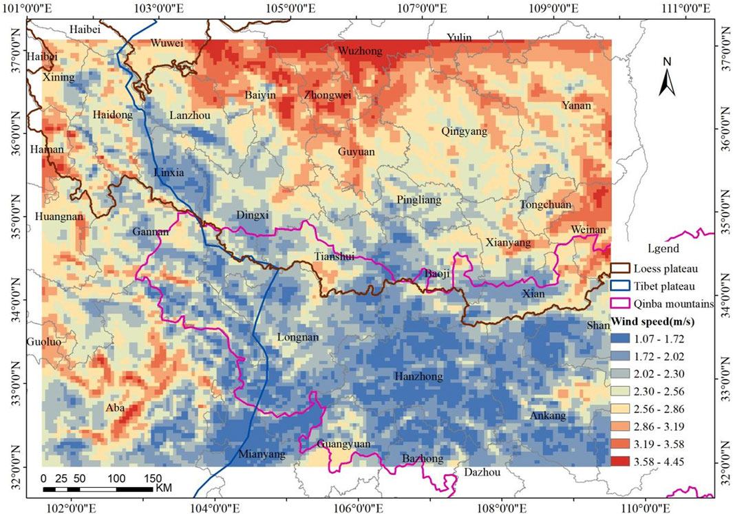
FIGURE 2. 5 km × 5 km annual mean 10-m wind speed in the study area in 2019.

FIGURE 3

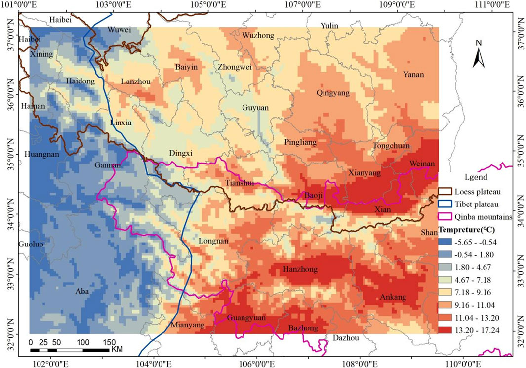
FIGURE 3. 5 km × 5 km annual mean ground temperature in the study area in 2019.

FIGURE 4

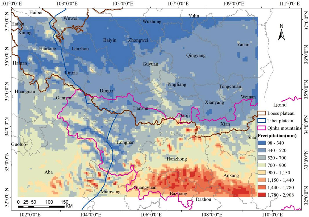
FIGURE 4. 5 km × 5 km precipitation in the study area in 2019.

Figure 2 clearly shows that the Loess Plateau has the highest u, particularly in areas around Baiyin, Zhongwei, and Wuzhong. The u is relatively lower on the Tibet Plateau and lowest on the Qinba Mountains. Figure 3 indicates that the annual mean temperature in the study area has an east-west and south-north gradient, with higher temperatures observed in the eastern and southern regions and lower temperatures in the western and northern areas. Owing to the “heat island effect,” the highest temperatures are concentrated in urban built-up areas. As depicted in Figure 4, the annual precipitation gradually decreases from south to north within the study area. The Qinba Mountains receive the most annual precipitation, followed by the Tibet Plateau, while the lowest precipitation is found on the Loess Plateau.

Because the three factors are overestimated to varying degrees, and the MFB of monthly precipitation is larger, part of the overestimation will be offset in the calculation of climate factors. The value of C for each grid cell in the study area can be calculated by Eqs 2.3, 2.4. Figure 5 illustrates the range of the C, which spans from a minimum of 0.0001 to a maximum of 1.227, with a mean value of 0.0586. These findings align closely with that of the magnitudes reported by Li et al. (2020) for different districts across Beijing. The distribution of C in the study area is uneven, with the highest values being found for the Loess Plateau, particularly in the northern areas around Baiyin, Zhongwei, and Wuzhong. The Tibet Plateau follows, exhibiting relatively higher C values, primarily in areas such as Haidong, Hainan, and Huangnan prefectures. Conversely, the lowest C values are observed in the Qinba Mountains. The primary factors contributing to the variation in the distribution of C are the 10-m wind speed and precipitation. In the northern part of the Loess Plateau, the terrain is relatively flat, resulting in higher 10-m wind speed. However, this region falls within a semi-arid and arid zone, resulting in relatively lower precipitation. Furthermore, Figure 5 indicates that even within the same city or county-level administrative area, there are certain variations in C among grid cells, with high values typically absent in urban built-up areas.

FIGURE 5

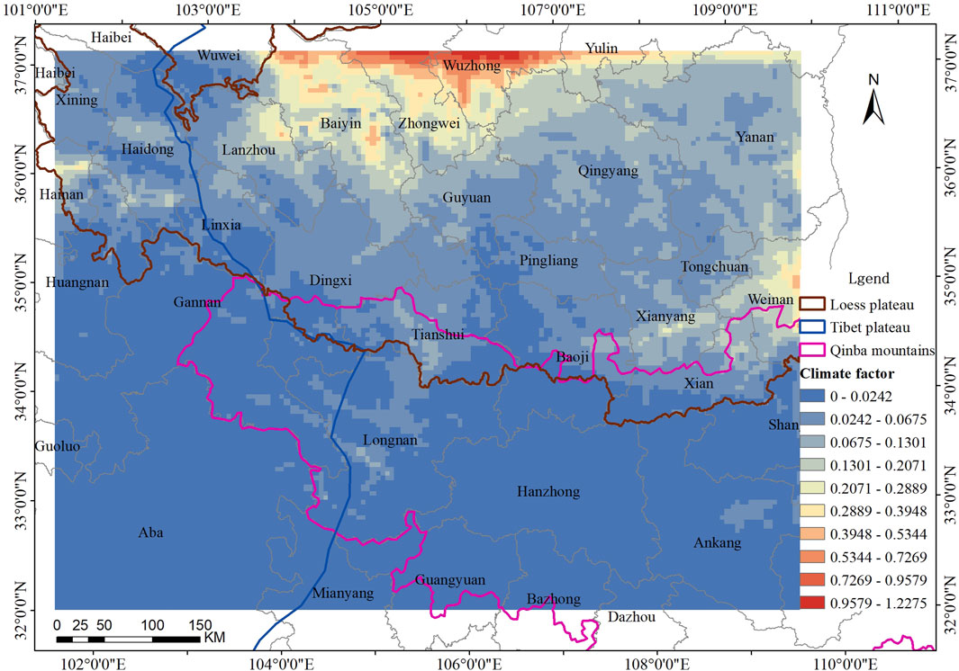
FIGURE 5. 5 km × 5 km climate factor of the study area in 2019.

3.1.2 Vegetation cover factor

In this study, we used the 2019 MODIS MCD12Q1 product to calculate the spatial distribution of VC values for each month, as well as the distribution of annual mean VC values. Figure 6 illustrates the VC values for representative months and the overall year. Different land use types, such as forests, grasslands, deserts, and croplands (including crops), feature diverse vegetation types. Natural vegetation has different growth cycles, and agricultural crops have varying periods for planting, growth, and harvesting. Consequently, the VC values vary each month for different land use types. As depicted in Figure 6, the VC values exhibit variations across months, regions, and grid points. On the Loess Plateau, the VC values are the lowest among the three regions, with the minimum values occurring in July and August. This decline may be primarily attributed to winter wheat harvesting (Qi et al., 2022). The Tibet Plateau exhibits intermediate VC values, with the lowest value being observed in March, when grasses wither till April (Zhuo et al., 2018). In contrast, the Qinba Mountains exhibit the highest VC values, with the lowest value being observed in June, possibly associated with the harvest of economic crops such as rapeseed (oil crop) and vegetables (Xiao, 2022; Chen et al., 2023).

FIGURE 6

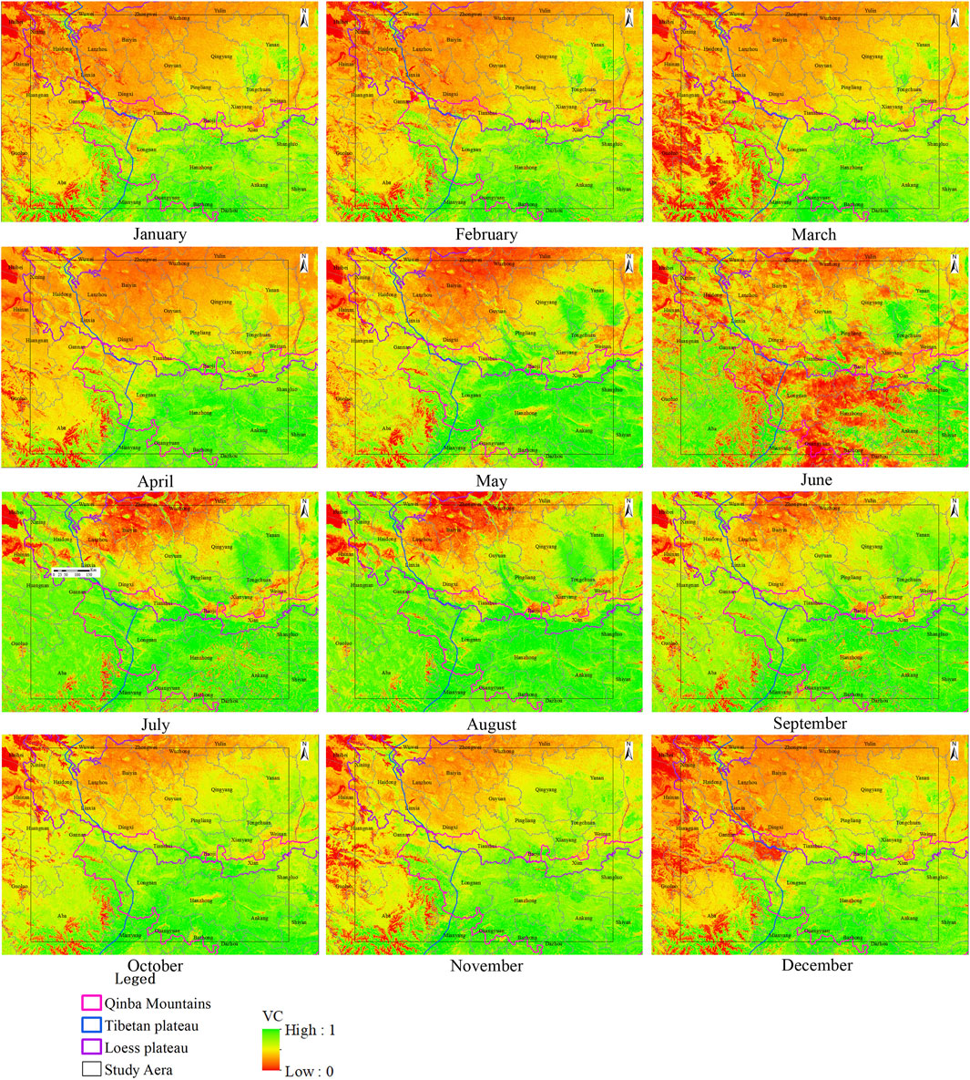
FIGURE 6. Monthly mean VC (250 m × 250 m) in the study area of Western China in2019.

In areas of urban construction, fugitive dust emissions mainly arise from road and construction activities, while stockpile dust appear around industries and mining facilities, and FSD outside urban built-up areas. FSD regions are typically located outside urban built-up areas, and water areas and rice paddies are generally considered non-FSD regions (Ministry of Environmental Protection, 2014). Therefore, construction areas, water areas, and paddy fields are categorized as non-sources for FSD in this study using the LUCC data (Xu et al., 2018).

Furthermore, Zhao, (2006) conducted wind tunnel experiments on the Inner Mongolia grassland and reported that on places whose VC are above 40%, wind erosion does not occur even when the wind speed arrives at 10 m s⁻¹. Additionally, on high-VC grasslands where the VC reaches 60%–80%, wind erosion is effectively suppressed even when wind speed increases to 14–18 m s⁻¹. Furthermore, other Chinese researchers have suggested that when the NDVI exceeds 0.61, FSD emissions are considered negligible (Song et al., 2021). Accordingly, areas with VC values greater than 0.61 are also classified as non-sources for FSD. Having been optimized by GIS, the mean VC value in the study region comes to 0.5. Figure 7 provides a visual representation of the VC at a resolution of 1 km. Additionally, the mean V values, which represents the absence of vegetation, is calculated to be 0.33. As depicted in Figure 8, the distribution of V values at a 5-km resolution is opposite to that of VC, indicating areas with lower vegetation cover tend to have higher soil bareness.

FIGURE 7

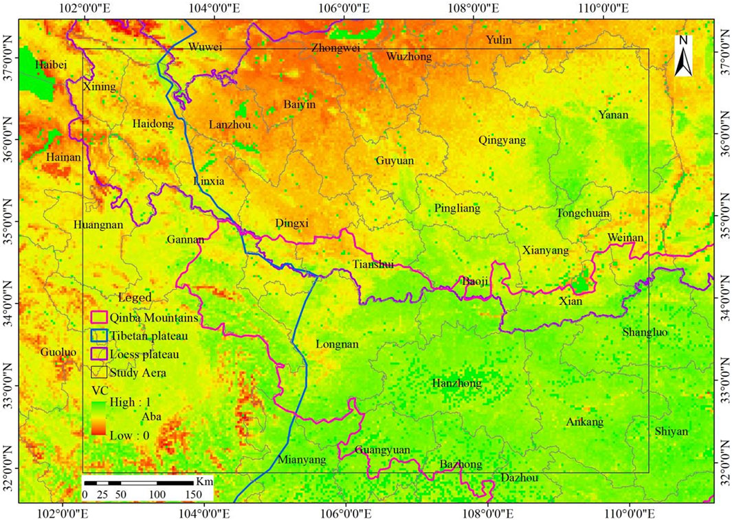
FIGURE 7. Optimized annual mean VC (1 km × 1 km) in the study area in 2019.

FIGURE 8

FIGURE 8. Annual mean V (5 km × 5 km) in the study area in 2019.

3.1.3 Wind erosion index

The Wind Erosion Index hinges on the soil texture type. In this study, we have cited the soil texture from the Chinese soil dataset (V1.1) provided by the Scientific Data Center for Cold and Arid Regions (http://westdc.Westgis.ac.cn), and referenced the I of many types from the “Technical Guidelines for the Compilation of Fugitive Dust Emission Inventories” (http://www.zhb.gov.cn/gkml/hbb/qt/201407/t20140714_276127.htm), thereby eliciting the distribution of soil texture and I in the whole area, as demonstrated in Table 2 and Figure 9.

TABLE 2

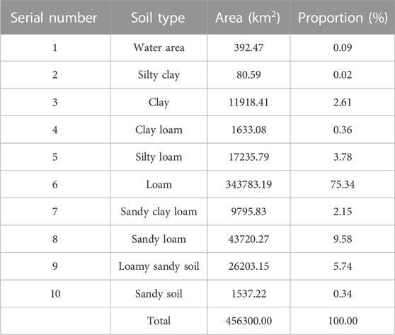
TABLE 2. Proportion of soil types in the study area.

FIGURE 9

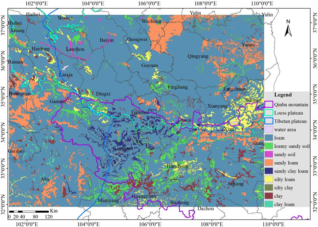
FIGURE 9. Soil types in the study area in Western China.

The study area encompasses nine soil typesl, with loam being the most widely distributed, especially on the Loess Plateau, and exhibiting the highest wind erosion index, accounting for 75.34% of the whole. Sandy loam constitutes 9.58% of the study area and is distributed across various regions, notably Wuzhong City in Ningxia Autonomous Region, Qingyang City, and Gannan Prefecture in Gansu Province, as well as Huangnan Prefecture in Qinghai Province. Loamy sandy soil represents 5.74% of the area and is primarily distributed on the Qinba Mountains. Silty loam occupies 3.78% and is primarily concentrated in Xi’an and Weinan cities in Shaanxi Province. Sandy clay loam, characterized by high wind erosion index, is less prevalent and primarily concentrated in the Qinba Mountains. Additionally, small water areas account for 0.09% of the study area, as indicated in Table 2 and Figure 9.

The reference values for wind erosion index provided by the “Technical Guidelines for the Compilation of Fugitive Dust Emission Inventories” show a consistent ratio of 1:0.3:0.05 for TSP, PM10, and PM2.5 across various soil types, respectively. Therefore, the distribution of I value for TSP, PM10, and PM2.5 in the study area is consistent. In this study, the I value is assigned to the 1 km × 1 km resolution soil types, and GIS geometric calculations are conducted to derive the distribution of I for TSP at a resolution of 5 km × 5 km, as detailed in Figure 10. In this study, TSP has been analyzed as an example. The wind erosion index of the Loess Plateau is the highest in the study area, reaching 911t·(hm2•a)−1, primarily found in regions with loam distribution. The Tibet Plateau followed, and the Qinba Mountain has the lowest, as low as 6.4t·(hm2•a)−1.

FIGURE 10

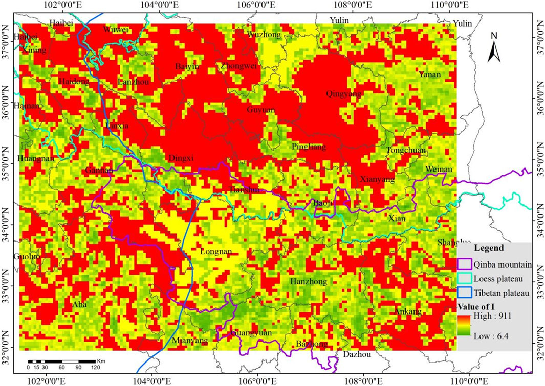
FIGURE 10. Wind erosion index (TSP) of the study area in Western China.

3.1.4 Remaining parameters setup

In addition to the parameters motioned above, there are two remaining parameters in the WEQ model: K and L. K represents the surface roughness factor and has a value of 0.5. However, in coastal, island, lakeside, and desert regions, the value of K is set at 1. This adjustment accounts for the different surface characteristics and their influence on wind erosion.

The parameter L denotes the unshielded width factor, representing the maximum distance without significant barriers (such as buildings or tall trees). The value of L depends on the width of the unshielded area. In the model, three categories are defined based on the unshielded width: (1) When the unshielded width is ≤ 300 m, L = 0.7. (2) For unshielded width between 300 m and 600 m, L = 0.85. (3) When the unshielded width is ≥ 600 m, L = 1.0.

In this study, the croplands in the western region included in this study are primarily dry lands and are predominantly flat. They are surrounded by protective forests; therefore, the K value was set at 0.5 and the L value at 0.7. For grasslands with medium and low VC, the K value is also set at 0.5, and the L value is considered as the intermediate value of 0.85, indicating a wider unshielded width compared to croplands. In sandy areas, deserts, saline-alkali lands, bare soil, and rocky terrain, both K and L values are set at 1.0. This reflects the high surface roughness and the absence of significant barriers, as these areas are more prone to wind erosion.

3.2 Spatial distribution

Based on calculations, the annual TSP emissions in the study area for the year 2019 amounted to 983.59 kt/a, PM₁₀ emissions totaled 2950.8 kt/a, and PM_2.5 emissions were recorded as 491.8 kt/a. As TSP, PM₁₀, and PM_2.5 have the same scale factor, their spatial distribution patterns in the study area are consistent. For the purpose of spatial distribution analysis, PM_2.5 has been selected as an example. A 5 km-resolution grid-based FSD emission inventory for PM_2.5 was generated for the year 2019, based on the corresponding parameters, as depicted in Figure 11 and Table 3.

FIGURE 11

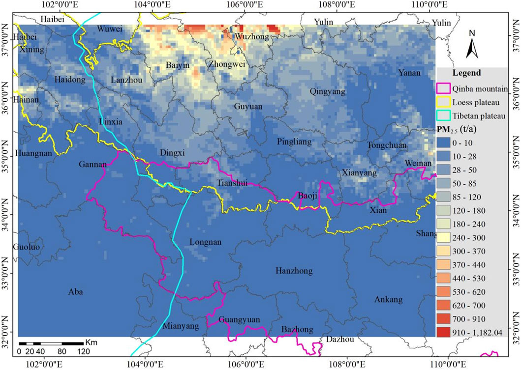
FIGURE 11. PM_2.5 from FSD in the study area in Western China in 2019.

TABLE 3

TABLE 3. Comparison of FSD emission intensity between the study area and other regions.

The results reveal that the regions with the highest PM_2.5 emissions from FSD and emission intensity in the study area are primarily located in the Loess Plateau. In 2019, the PM_2.5 emissions in this area amounted to 474.72 kt, accounting for 96.53% of the entire study area. The FSD-source areas covered approximately 191,304.4 km², resulting in an emission intensity of 2.48 t/km². Notably, the key emission hotspots are concentrated in the northern part of the study area, including Baiyin City of Gansu Province and Zhongwei and Wuzhong cities of Ningxia Autonomous Region. Moreover, the maximum emission in a 5 km × 5 km grid reached 1,182.04 t.

The FSD emissions in the Tibet Plateau ranked second, with total PM_2.5 emissions of 35.75 kt in 2019, constituting 7.27% of the entire study area. The FSD-source areas covered approximately 98,993.1 km², resulting in an emission intensity of 0.36 t/km². The key emission hotspots were identified in the northwestern part of the study area, specifically in Huangnan and Haidong prefectures of Qinghai Province. In a 5 km × 5 km grid, the maximum emission of Tibet Plateau reached 331.2t.

On the other hand, the FSD emissions in the Qinba Mountains were relatively lower than the former two regions, with total PM_2.5 emissions of 11.94 kt in 2019, accounting for 2.43% of the entire study area. The FSD-source areas covered approximately 35,977.51 km², resulting in an emission intensity of 0.33 t/km². The highest emission intensity was observed in the northeastern part of Xi’an City and the southern part of Weinan City of Shaanxi Province. For Qinba Mountains, its maximum emission in a 5 km × 5 km grid in 2019 was 72.82t. The total emissions from the Tibet Plateau, Loess Plateau, and Qinba Mountains are higher than the total emissions in the study area owing to a few overlapping areas.

Moreover, a comparison was conducted between the soil dust emissions in the study area and other regions in China using PM_2.5 as a reference. The comparison considered emissions quantity, FSD-source areas, and emission intensity, as presented in Table 3. From Table 3, it can be observed that the emission intensity of PM_2.5 in the Beijing–Tianjin–Hebei region and Hebei Province is relatively consistent. Surprisingly, in the study area, the emission intensity of PM_2.5 from FSD exceeds that of Beijing–Tianjin–Hebei and Hebei Province by three times. This significant difference is primarily attributed to the high emission intensity of 2.48 t/km² on the Loess Plateau, which is approximately five times that of the Beijing–Tianjin–Hebei region, resulting in elevated emission intensity levels in the study area. Meanwhile, the Tibet Plateau and Qinba Mountains exhibit lower FSD emission intensities of only 0.36 and 0.33 t/km², respectively, owing to their higher VC and precipitation levels. Both these values are lower than those estimated in the Beijing–Tianjin–Hebei region. The higher FSD emission intensity in the study area, particularly on the Loess Plateau, compared with the Beijing–Tianjin–Hebei region, to factors such as lower VC and precipitation levels, higher wind speed and wind erosion index, all of which are prevalent in the study area because of its comparable latitude and similar annual mean temperature variations with the Beijing–Tianjin–Hebei region.

3.3 Temporal distribution characteristics

In the WEQ model, the estimation of wind erosion is typically based on annual mean statistics, which may not account for variations in wind erosion potential across different months of the year. However, in this study, it was observed that the variations between different months are primarily influenced by climate factors and vegetation cover, which are also the main drivers of fluctuations in FSD emissions throughout the year. Additionally, Skidmore and Woodruff (1968) suggested using the annual PE to compute monthly climate factor. Therefore, To address this limitation and capture the monthly variations in wind erosion potential, we proposed to calculate the monthly allocation coefficients using the V and C values for each grid and each month, as presented in Eq. 2.11.

${\mathrm{k}}_{\text{ij}}={\mathrm{V}}_{\text{ij}}\times {\mathrm{u}}_{\text{ij}}^3/{\left\{{\left[{\mathrm{P}}_{\mathrm{i}}/\left(1.8{\mathrm{T}}_{\text{ij}}+22\right)\right]}^{10/9}\right\}}^2(2.11)$

Where, k_ij represents the distribution coefficient for grid i in month j. V_ij represents the V value for grid i in month j. u_ij is the monthly mean 10-m wind speed for grid i in month j. P_ij is the cumulative precipitation for grid i in month j. T_ij is the monthly mean ground temperature for grid i in month j.

By using Eq. 2.7 we calculated the allocation coefficients for each grid within the study area for the year 2019. These coefficients were then normalized and combined with the annual emission distribution to determine the monthly emissions of PM_2.5 from FSD in each grid during that year, as shown in Table 6. In our study, we computed the values for each grid separately due to the variations in C and V across different months. Figure 12 illustrates the monthly distribution of PM_2.5 emissions from FSD, highlighting the variations observed for each grid.

FIGURE 12

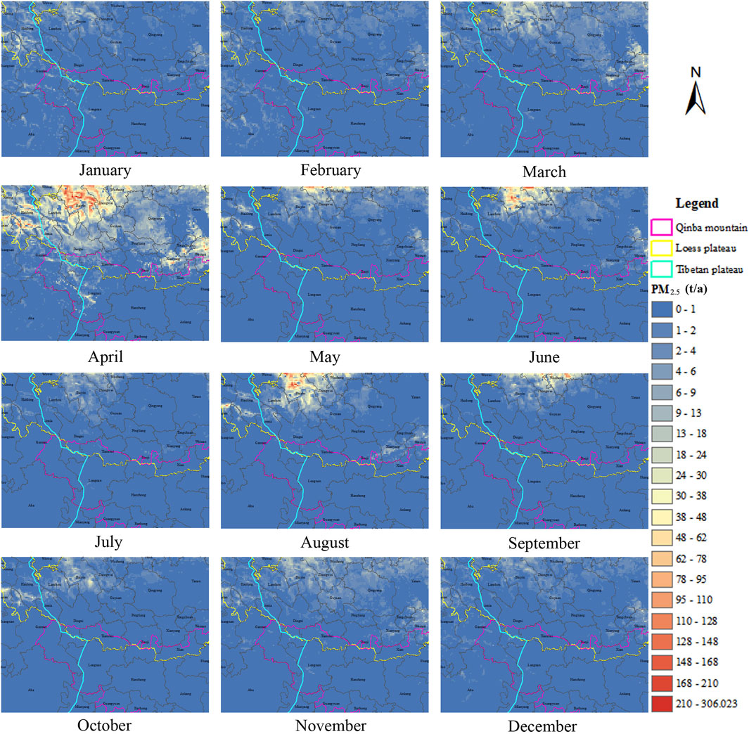
FIGURE 12. Fugitive Soil dust levels in the study area in Western China in 2019.

Based on the results presented in Table 4, the PM_2.5 emissions from FSD in the study area exhibits significant non-linear monthly variations. The highest emissions occur in April, accounting for 36.21% of the total annual emissions. The second and third highest emissions are in August and June, respectively. These variations are primarily because the northern region of the study area is part of the Loess Plateau and located in a semi-arid zone. During the summer months, the ground temperature increases without a significant increase in precipitation, leading to higher emissions. On the other hand, the lowest emissions are observed in July.

TABLE 4

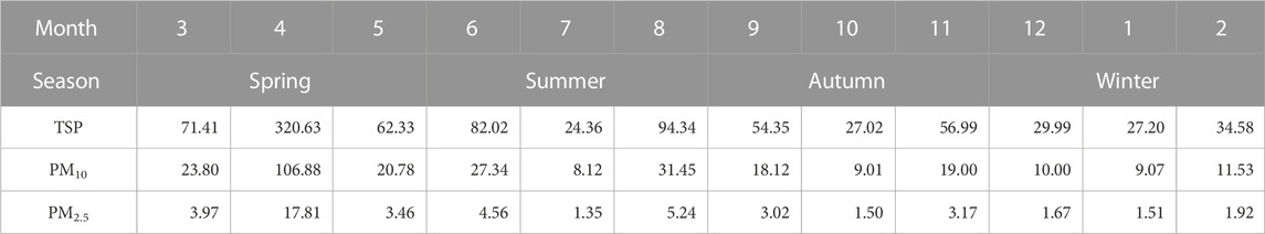
TABLE 4. Overview of PM_2.5 emissions from FSD in the study area for January to December in 2019 Unit: t.

When considering the seasonal distribution, spring demonstrates the most significant PM_2.5 emissions from FSD in the study area, accounting for 51.32% of the total annual emissions. Summer follows with 22.67%, and autumn with 15.64%. Winter exhibits the lowest emissions, accounting for only 10.37% of the total annual emissions. Overall, the emission pattern exhibits a seasonal trend of spring > summer > autumn > winter. The high emissions observed during spring, summer, and autumn primarily occur on the Loess Plateau, influenced by low precipitation and poor VC in the region. Conversely, emissions from the Tibet Plateau increase proportionately during winter.

Based on Figure 12, the primary areas for PM_2.5 emissions from FSD in the study area are identified as Baiyin City in Gansu Province, and Zhongwei and Wuzhong cities in the Ningxia Autonomous Region. These areas consistently exhibit high emissions throughout the months in 2019, primarily due to factors such as high wind speed, poor vegetation coverage, and low precipitation. These conditions contribute to increased wind erosion and subsequent PM_2.5 emissions from FSD.

Xianyang and Weinan cities of Shaanxi Province represent the secondary emission source areas on the Loess Plateau. The PM_2.5 emissions from FSD exhibit a gradually increasing trend from January to April, followed by a fluctuant decrease from April to September, reaching its lowest level in September, and then a subsequent increase from October to December. This pattern aligns with local agricultural activities, as described in Qi et al. (2022).

In parts of the Tibet Plateau, PM_2.5 emissions from FSD remain relatively constant in January and February, decrease in March, increase in April, gradually decline from April to September, and start to rise again from October to December These emission patterns are closely associated with agricultural and pastoral practices in the region, as mentioned in Zhuo et al. (2018). The overall emission levels on the Qinba Mountains are low, with the primary emission areas situated in the southern parts of Xi’an and Weinan cities.

3.4 Uncertainty analysis

The uncertainty in the emission inventories for certain atmospheric pollution stems primarily from the calculation and selection of activity levels and emission factors (Zhong et al., 2007). In this study, the uncertainty involved in the FSD emission inventory can be attributed primarily to the following factors: 1. The climate factors were simulated using the WRF model, and the simulation results may thus deviate from the actual conditions, causing the uncertainty of the estimation results. 2. The MODIS MOD13Q1 product provides remote sensing image data at 16-day intervals. In this study, the mean VC for a specific month was calculated using the 16-day images. However, this approach may introduce discrepancies compared to the actual values. 3. The wind erosion index and particle size multiplier were referenced from the “Technical Guidelines for the Compilation of Fugitive Dust Emission Inventories (Trial)”, without conducting specific particle size sampling and analysis for different soil types, thereby introducing certain uncertainties.

4 Conclusion

Compared to existing studies on Wind Erosion Quantity, our research takes the convergent areas of the Loess Plateau, Tibet Plateau, and Qinba Mountains as a case study to estimate FSD emissions. We have introduced innovative approaches, such as utilizing WRF simulated data to calculate climate factors, optimizing the vegetation cover factor using NDVI and LUCC data, and establishing improved criteria for calculating the monthly allocation coefficients. The results of our study reveal the following key findings:

1) The study area is located in the convergence areas of the Tibet Plateau, Loess Plateau, and Qinba Mountains. Due to the influence of topography and monsoons, meteorological factors, including wind speed, precipitation, and temperature, exhibit uneven distribution. Using weather station data to calculate FSD emissions may introduce deviations from reality. By employing ERA5 reanalysis data to drive the WRF model, our study found that the maximum, minimum, and mean climate factor values in the study area are 0.8601, 0.0000764, and 0.0388, respectively.

2) After the optimization process, which involved excluding construction land, water areas, paddy fields, and regions with VC values greater than 0.61 as FSD emissions, the mean soil bareness (V) in the study area for 2019 was determined to be 0.33. Moreover, VC and V values for different land use types across different months exhibit non-linear variations due to the influence of regional background and agricultural and pastoral activities.

3) In 2019, the annual TSP, PM10, and PM2.5 from FSD emissions in the study area amounted to 9835.9, 2950.8, and 491.8 kt/a, respectively. The highest FSD emissions and emission intensity were observed on the Loess Plateau, particularly in the northern part of the study area, including Baiyin City of Gansu Province, and Zhongwei and Wuzhong cities of Ningxia Autonomous Region. The Tibet Plateau had the second-highest FSD emissions, primarily concentrated in the northwestern part of Qinghai Province, particularly in Huangnan and Haidong prefectures. The Qinba Mountains exhibited the lowest overall FSD emissions.

4) The monthly allocation coefficients is mainly influenced by climate factor and vegetation cover factor. Climate factor is determined by meteorological conditions, while vegetation cover factor is associated with agricultural and pastoral activities. The monthly allocation coefficients, climate factor, and vegetation cover factor for each grid demonstrate non-linear patterns. In the study area for 2019, April had the highest FSD emissions, accounting for 36.21% of the total annual emissions. Following closely were August and June, ranked as the second and third highest emission months, respectively. These patterns can be attributed to the arid and semi-arid conditions experienced in the primary emission source area, the northern part of the Loess Plateau, during summer. During this season, ground temperatures rise without significant increases in precipitation and vegetation coverage, resulting in elevated FSD emissions.

Data availability statement

Publicly available datasets were analyzed in this study. This data can be found here: ERA5: https://cds.climate.copernicus.eu/cdsapp#!/home; NDVI: https://modis.gsfc.nasa.gov/; LUCC: https://www.resdc.cn/Harmonized World Soil Database: http://www.ncdc.ac.cn. Surface meteorological observation data: http://data.cma.cn/data/detail/dataCode/A.0012.0001.html.

Author contributions

PW: Methodology, Writing–original draft, Formal Analysis. MC: Writing–original draft, Writing–review and editing. WA: Data curation, Writing–original draft. YL: Data curation, Writing–original draft. FP: Writing–review and editing.

Funding

The author(s) declare financial support was received for the research, authorship, and/or publication of this article. Supported by Special funds for basic scientific research operations of central universities: Source analysis of PM_2.5 and formation mechanism of secondary organic aerosol in Lanzhou City (No. lzujbky-2017-66).

Acknowledgments

Supported by Supercomputing Center of Lanzhou University.

Conflict of interest

The authors declare that the research was conducted in the absence of any commercial or financial relationships that could be construed as a potential conflict of interest.

Publisher’s note

All claims expressed in this article are solely those of the authors and do not necessarily represent those of their affiliated organizations, or those of the publisher, the editors and the reviewers. Any product that may be evaluated in this article, or claim that may be made by its manufacturer, is not guaranteed or endorsed by the publisher.

References

Apte, J. S., Marshall, J. D., Cohen, A. J., and Brauer, M. (2015). Addressing global mortality from ambient PM_2.5. Environ. Sci. Technol. 49, 8057–8066. doi:10.1021/acs.est.5b01236

PubMed Abstract | CrossRef Full Text | Google Scholar

Asian Clean Air Center (2021). Available at: http://www.allaboutair.cn/a/reports/2021/1027/622.html (Accessed July 12, 2023).

Bi, X., Feng, Y., Wu, J., Wang, Y., and Zhu, T. (2007). Source apportionment of PM₁₀ in six cities of northern China. Atmos. Environ. 41, 903–912. doi:10.1016/j.atmosenv.2006.09.033

CrossRef Full Text | Google Scholar

Buschiazzo, D. E., and Zobeck, T. M. (2008). Validation of WEQ, RWEQ and WEPS wind erosion for different arable land management systems in the Argentinean Pampas. Earth Surf. Process. Landforms 33, 1839–1850. doi:10.1002/esp.1738

CrossRef Full Text | Google Scholar

Chen, G. P., Sun, X. M., Li, Y., Xue, Y., Xing, L. H., Xi, G. Q., et al. (2023). Development status and suggestions of rapeseed industry in Hanzhong. Tillage Cultiv. 43 (1), 146–148. doi:10.13605/j.cnki.52-1065/s.2023.01.031

CrossRef Full Text | Google Scholar

Cheng, N., Zhang, D., Li, Y., Xie, X., Chen, Z., Meng, F., et al. (2017). Spatio-temporal variations of PM_2.5 concentrations and the evaluation of emission reduction measures during two red air pollution alerts in Beijing. Sci. Rep. 7, 8220. doi:10.1038/s41598-017-08895-x

PubMed Abstract | CrossRef Full Text | Google Scholar

Chepil, W. S. (1958). Soil conditions that influence wind erosion. AgEcon Search. Technical Bulletins 157333. . doi:10.22004/ag.econ.157333

CrossRef Full Text | Google Scholar

Countess Environmental,BonifacioH. F.MaghirangR. G.TrabueS. L. (2006). WRAP fugitive dust handbook. Prepared by countess environmental, westlake village. Calif., for western governors’ association. Denver. Colo Sept.7.

Cowherd, C., Axetell, K., Guenther, C. M., and Jutze, G. A. (1974). Development of emission factors for fugitive dust sources. National Service Center for Environmental Publications (NSCEP). EPA-450/3-74-037.

Google Scholar

Craig, D. C., and Turelle, J. W. (1964). Guide for wind erosion control on cropland in the great plains States, soil conservation service, 104. Washington, D.C.: U.S. Department of Agriculture, 41.

Google Scholar

Fryrear, D. W., Bilbro, J. D., Saleh, A., Schomberg, H., Stout, J. E., and Zobeck, T. M. (2000). RWEQ: improved wind erosion technology. J. Soil Water Conservation 55, 183–189.

Google Scholar

Fu, X., Wang, S., Zhao, B., Xing, J., Cheng, Z., Liu, H., et al. (2013). Emission inventory of primary pollutants and chemical speciation in 2010 for the Yangtze River Delta region, China. Atmos. Environ. 70, 39–50. doi:10.1016/j.atmosenv.2012.12.034

CrossRef Full Text | Google Scholar

Gitelson, A. A., Kaufman, Y. J., Stark, R., and Rundquist, D. (2002). Novel algorithms for remote estimation of vegetation fraction. Rem. Sens. Environ. 80 (1), 76–87. doi:10.1016/S0034-4257(01)00289-9

CrossRef Full Text | Google Scholar

Gregory, J. M., Wilson, G. R., Singh, U. B., and Darwish, M. M. (2004). TEAM: integrated, process-based wind-erosion model. Environ. Model. Softw. 19, 205–215. doi:10.1016/S1364-8152(03)00124-5

CrossRef Full Text | Google Scholar

Guo, X., Feng, H. B., and Lu, Y. J. (2017). Estimation of emissions of PM_2.5 from soil dust in Hebei Province. J. Industrial Sci. Technol. 34 (6), 477–482. doi:10.7535/hbgykj.2017yx06015

CrossRef Full Text | Google Scholar

Ji, D., Deng, Z., Sun, X., Ran, L., Xia, X., Fu, D., et al. (2020). Estimation of PM_2.5 mass concentration from visibility. Adv. Atmos. Sci. 37, 671–678. doi:10.1007/s00376-020-0009-7

CrossRef Full Text | Google Scholar

Jia, K., Yao, Y. J., Wei, X. Q., Gao, S., Jiang, B., and Zhao, X. (2013). A review on fractional vegetation cover estimation using remote sensing. Adv. Earth Sci. 28, 774–782. doi:10.11867/j.issn.1001-8166.2013.07.0774

CrossRef Full Text | Google Scholar

Jutze, G., and Axetell, K. (1974). Investigation of fugitive dust, Vol. 1 - Sources. National Service Center for Environmental Publications (NSCEP). EPA-450/3-74-036-a.Emissions and control

Google Scholar

Jutze, G., and Axetell, K. (1976). “Factors influencing emissions from fugitive dust,” in Symposium on fugitive emission measurement and control (Hartford, CT: National Service Center for Environmental Publications (NSCEP)).

Google Scholar

Li, B.-B., Huang, Y.-H., Bi, X.-H., Liu, L.-Y., and Qin, J.-P. (2020). Localization of soil wind erosion dust emission factor in beijing. Environ. Sci. 41, 2609–2616. doi:10.13227/j.hjkx.201908243

PubMed Abstract | CrossRef Full Text | Google Scholar

Li, T., Bi, X., Dai, Q., Wu, J., Zhang, Y., and Feng, Y. (2021). Optimized approach for developing soil fugitive dust emission inventory in "2+26" Chinese cities. Environ. Pollut. 285, 117521. doi:10.1016/j.envpol.2021.117521

PubMed Abstract | CrossRef Full Text | Google Scholar

Liu, A. B., Wu, Q. Z., Chen, Y. T., Zhao, T. C., and Cheng, X. (2018). Estimation of dust emissions from bare soil erosion over beijing plain area. Zhongguo Huanjing Kexue/China Environ. Sci. 38 (2), 471–477. doi:10.19674/j.cnki.issn1000-6923.2018.0054

CrossRef Full Text | Google Scholar

Liu, H., Wu, B., Liu, S., Shao, P., Liu, X., Zhu, C., et al. (2018). A regional high-resolution emission inventory of primary air pollutants in 2012 for Beijing and the surrounding five provinces of North China. Atmos. Environ. 181, 20–33. doi:10.1016/j.atmosenv.2018.03.013

CrossRef Full Text | Google Scholar

Liu, J., Han, Y., Tang, X., Zhu, J., and Zhu, T. (2016). Estimating adult mortality attributable to PM_2.5 exposure in China with assimilated PM_2.5 concentrations based on a ground monitoring network. Sci. Total Environ. 568, 1253–1262. doi:10.1016/j.scitotenv.2016.05.165

PubMed Abstract | CrossRef Full Text | Google Scholar

Liu, Q., Guo, Z. L., Chang, C. P., Wang, R. D., Li, J. F., Li, Q., et al. (2021). Potential wind erosion simulation in the agro-pastoral ecotone of northern China using RWEQ and WEPS models. J. Desert Res. 41, 27–37. doi:10.7522/j.issn.1000-694X.2020.00122

CrossRef Full Text | Google Scholar

Lu, L., and Liu, C. (2019). Chinese soil data set based on world soil database (hwsd) (v1.1). National Cryosphere Desert Data Center. doi:10.12072/ncdc.westdc.db3647.2023

CrossRef Full Text | Google Scholar

Lyles, L. (1983). Erosive wind energy distributions and climatic factors for the West. J. Soil Water Conserv. 38 (2), 106–109.

Google Scholar

Mandakh, N., Tsogtbaatar, J., Dash, D., and Khudulmur, S. (2016). Spatial assessment of soil wind erosion using WEQ approach in Mongolia. J. Geogr. Sci. 26, 473–483. doi:10.1007/s11442-016-1280-5

CrossRef Full Text | Google Scholar

Ministry of Environmental Protection, (2014). Available at: https://www.mee.gov.cn/gkml/hbb/bgg/201501/t20150107_293955.htm (Accessed July 12, 2023).

Panebianco, J., and Buschiazzo, D. (2008). Erosion predictions with the Wind Erosion Equation (WEQ) using different climatic factors. Land Degrad. Dev. 19, 36–44. doi:10.1002/ldr.813

CrossRef Full Text | Google Scholar

Qi, J., Zheng, B., Li, M., Yu, F., Chen, C., Liu, F., et al. (2017). A high-resolution air pollutants emission inventory in 2013 for the Beijing-Tianjin-Hebei region, China. Atmos. Environ. 170, 156–168. doi:10.1016/j.atmosenv.2017.09.039

CrossRef Full Text | Google Scholar

Qi, Y., Zhang, Q., Hu, S. J., Cai, D. H., Zhao, F. N., Chen, F., et al. (2022). Climate change and its impact on winter wheat potential productivity of Loess Plateau in China. Ecol. Environ. Sci. 31 (8), 1521–1529. doi:10.16258/j.cnki.1674-5906.2022.08.003

CrossRef Full Text | Google Scholar

Shang, X., Zhang, K., Meng, F., Wang, S., Lee, M., Suh, I., et al. (2018). Characteristics and source apportionment of fine haze aerosol in Beijing during the winter of 2013. Atmos. Chem. Phys. 18, 2573–2584. doi:10.5194/acp-18-2573-2018

CrossRef Full Text | Google Scholar

Shao, Y. P., Raupach, M. R., and Leys, J. F. (1996). A model for predicting aeolian sand drift and dust entrainment on scales from paddock to region. Soil Res. 34, 309–342. doi:10.1071/sr9960309

CrossRef Full Text | Google Scholar

Skidmore, E. L. (1986). Soil erosion by wind: an Overview. Dordrecht: Springer.

Google Scholar

Skidmore, E. L., and Woodruff, N. P. (1968). Wind erosion forces in the United States and their use in predicting soil loss. United States: Agriculture handbook. Department of Agriculture no. 346.

Google Scholar

Song, H., Zhang, K., Piao, S., and Wan, S. (2016). Spatial and temporal variations of spring dust emissions in northern China over the last 30 years. Atmos. Environ. 126, 117–127. doi:10.1016/j.atmosenv.2015.11.052

CrossRef Full Text | Google Scholar

Song, L., Li, T., Bi, X., Wang, X., Zhang, W., Zhang, Y., et al. (2021). Construction and dynamic method of soil fugitive dust emission inventory with high spatial resolution in beijing-tianjin-hebei region. Res. Environ. Sci. 34 (8), 1771–1781. doi:10.13198/j.issn.1001-6929.2021.05.03

CrossRef Full Text | Google Scholar

Taylor, K. E. (2001). Summarizing multiple aspects of model performance in a single diagram. J. Geophys. Res. Atmos. 106 (D7), 7183–7192. doi:10.1029/2000JD900719

CrossRef Full Text | Google Scholar

The State Council (2013). Available at: http://www.gov.cn/zwgk/2013-09/12/content_2486773.htm (Accessed July 12, 2023).

The State Council (2018). Available at: http://www.gov.cn/zhengce/content/2018-07/03/content_5303158.htm (Accessed July 12, 2023).

US. Environmental Protection Agency (1977). Guideline for development of control strategies in areas with fugitive dust problems. Triangle Park, North Carllina: S. Environmental Protection Agency.

Google Scholar

Wang, S., Wang, T., Shi, R., and Tian, J. (2014). Estimation of different fugitive dust emission inventory in Nanjing. J. Univ. Chin. Acad. Sci. 31, 351–359. doi:10.7523/j.issn.2095-6134.2014.03.009

CrossRef Full Text | Google Scholar

Woodruff, N. P., and Siddoway, F. H. (1965). A wind erosion equation. Soil Sci. Soc. Am. J. 29, 602–608. doi:10.2136/sssaj1965.03615995002900050035x

CrossRef Full Text | Google Scholar

Xiao, Y. (2022). Temporal and spatial changes and prediction of carbon budget in palnting and animal husbandry in Guangyuan during the last 25 years. Sichuan Normal University. Master’s thesis.

Google Scholar

Xu, X., Liu, J., Zhang, S., Yan, C., and Wu, s (2018). Data from Remote sensing data set of multi-period land use monitoring in China (CNLUC). Resource and environmental science data registration and publication system. http://www.resdc.cn/DOI/doi.aspx?DOIid=54.

Google Scholar

Xu, Y. Q., Jiang, N., Yan, Q., Zhang, R. Q., Chen, L. F., and Li, S. S. (2016). Research on emission inventory of bareness wind erosion dust in zhengzhou. Environ. Pollut. Control. doi:10.15985/j.cnki.1001-3865.2016.04.005

CrossRef Full Text | Google Scholar

Xuan, J., Liu, G., and Du, K. (2000). Dust emission inventory in Northern China. Atmos. Environ. 34, 4565–4570. doi:10.1016/S1352-2310(00)00203-X

CrossRef Full Text | Google Scholar

Zhang, G., Liu, J., Zhang, Z., Zhao, X., and Zhou, Q. (2002). Spatial changes of wind erosion-caused landscapes and their relation with wind field in China. J. Geogr. Sci. 12, 153–162. doi:10.1007/BF02837469

CrossRef Full Text | Google Scholar

Zhang, Z., Gong, D., Mao, R., Kim, S. J., Xu, J., Zhao, X., et al. (2017). Cause and predictability for the severe haze pollution in downtown Beijing in November-December 2015. Sci. Total Environ. 592, 627–638. doi:10.1016/j.scitotenv.2017.03.009

PubMed Abstract | CrossRef Full Text | Google Scholar

Zhao, Y. L. (2006). Test and evaluation on influences of vegetation coverage on soil wind erosion by means of the movable wind tunnel. Inner Mongolia Agricultural University. Master’s thesis.

Google Scholar

Zheng, J., Zhang, L., Che, W., Zheng, Z., and Yin, S. (2009). A highly resolved temporal and spatial air pollutant emission inventory for the Pearl River Delta region, China and its uncertainty assessment. Atmos. Environ. 43, 5112–5122. doi:10.1016/j.atmosenv.2009.04.060

CrossRef Full Text | Google Scholar

Zhong, L. J., Zheng, J. Y., Louie, P., and Chen, J. (2007). Quantitative uncertainty analysis in air pollutant emission inventories: methodology and case study. Res. Environ. Sci. 20 (4), 15–20. doi:10.13198/j.res.2007.04.19.zhonglj.004

CrossRef Full Text | Google Scholar

Zhuo, G., Chen, S. R., and Zhou, B. (2018). Spatio-temporal variation of vegetation coverage over the Tibetan Plateau and its responses to climatic factors. Acta Ecol. Sin. 38 (9), 3208–3218. doi:10.5846/stxb201705270985

CrossRef Full Text | Google Scholar

Zou, X. Y., Zhang, C. L., Cheng, H., Kang, L. Q., Wu, X. X., Chang, C. P., et al. (2014). Classification and representation of factors affecting soil wind erosion in a Model. Adv. Earth Sci. 29 (8), 875–889. doi:10.11867/j.issn.10018166.2014.08.0875

CrossRef Full Text | Google Scholar