The impact of climate change policies on financial stability of China

Climate transition risks pose growing financial stability concerns, but research on quantifying climate policy impacts remains underexplored. This paper helps address this gap by evaluating how carbon tax (CT) and green supporting factor (GSF) influence China’s financial stability. An innovative dynamic stochastic general equilibrium (DSGE) model incorporating the banking sector is developed to quantify transmission channels, improving on conceptual studies. It reveals that more intense climate policies heighten impacts on financial stability, with CT improving it but GSF hampering it in the long run. However, both policies negatively affect stability initially, albeit insignificantly. These diagnostics underscore calibrating policy intensities and sequencing to balance climate and economic objectives. Furthermore, this study reveals asymmetric effects on polluting and non-polluting enterprises, with the former seeing reduced output and lending but the latter gaining. The differentiated approach proposed, tailored to firm emissions levels, provides key insights for unlocking smooth green transitions while maintaining financial system resilience. The paper makes important contributions by bringing together climate policies, adaptation, and financial stability. The findings offer insights into achieving a smooth climate transition while maintaining financial stability. Specific implications include starting with low CT on the heaviest emitters, gradually lowering risk weights for green lending, and using public incentives and investment to aid polluting firms’ transition. This study offers valuable quantitative insights for developing country-specific climate financial risk policies.

1 Introduction

As the world’s most complex environmental problem resulting in the largest externality, climate change has a broad and profound impacts (Tang Y. et al., 2023). It leads to a greater frequency of extreme weather events and an increasingly pronounced negative impact on the economic system which are manifested in a wide range of areas such as agriculture, industry, manufacturing, ecosystems and human health (World Bank, 2016; Bank, 2017; Duan et al., 2022; Tang W. et al., 2023; Duan et al., 2023). In addition, climate change-induced natural disasters have led to fluctuations in asset pricing, impacting the profitability and solvency of companies, increasing the credit risk, liquidity risk, and operational risk of the financial system and even posing a contagious risk, jeopardizing financial stability (Dietz et al., 2016; Lamperti et al., 2019; Liu et al., 2021).

To mitigate climate risk and enhance climate change resilience, nations have been implementing climate change policies (Cifuentes-Faura, 2022; Li et al., 2023; Liu et al., 2023). Carbon tax (CT) on carbon-intensive activities has been advocated to address climate change and the mispricing of climate-related financial risks. It is a binding policy that would raise production costs for carbon-intensive enterprises, encouraging low-carbon energy technology investments. However, concerns have been raised regarding its impact on inequality, financial stability, and GDP growth (Bovari et al., 2018; Mercure et al., 2018; Monasterolo and Raberto, 2018). China has included carbon tax (CT) in the Environmental Protection Tax Law, and CT policy will be levied in due course. This policy provides carbon-intensive firms with the choice of either paying extra taxes or investing in low-carbon energy technologies (Shang et al., 2023). The European Commission has proposed the revision of micro-prudential banking framework by including a green supporting factor (GSF) to reduce the need for additional capital when making green investments (Dombrovskis, 2018). It is a proposed incentive policy that would encourage financial institutions to support investments in ecologically friendly ventures. GSF can break the impasse of CT, but there are disputes on the possibility of increased financial risk and instability (Thoma and Hilke, 2018).

China faces particularly pressing climate policy imperatives (Yuan et al., 2023). First, China is one of the countries that are most vulnerable to climate change (IPCC, 2022). Increasing sea levels and extreme weather events have posed significant threats to China’s agriculture, transportation, infrastructure and so on. Second, climate change will disrupt international supply chains, impacting China’s domestic goods supply and commodities prices. This will also affect the performance of financial firms with portfolios vulnerable to climate-related risks, potentially leading to financial instability. Therefore, the Chinese government has put great emphasis on the implementation of climate change policies. The 14th Five-Year Plan and the outline of the 2035 Vision propose reducing energy use and CO₂ emissions per unit of GDP by 13.5% and 18.0%, respectively. These policies emphasize carbon reduction and accelerate green transformation. Irrational green transitions, however, could threaten financial stability and perhaps lead to financial problems. Additionally, it has an impact on achieving the Sustainable Development Goals (SDGs), which include responsible consumption and production of affordable, dependable, and clean energy, technological innovation in response to climate change, and sustainable economic growth (SDGs 7, 8, 9, 12, and 13) (Monasterolo and Raberto, 2018; Lorente et al., 2023; Uche et al., 2023; Wang et al., 2023). Therefore, analyzing the impact of implementing CT and GSF on China’s financial system stability during the low-carbon economic transition is essential. This analysis helps in formulating effective policies for financial stability and achieving the SDGs.

This research offers a significant contribution by conducting a comprehensive analysis of the complex relationships among climate policies, financial stability, and economic performance. Despite growing concerns about climate transition risks, quantitative analysis of policy impacts on financial stability remains limited. This study presents a novel dynamic stochastic general equilibrium (DSGE) model that incorporates the banking sector. It provides a detailed analysis of the mechanisms by which carbon tax and green supporting factor policies impact both the real economy and the banking system. The findings reveal differentiated effects on polluting versus non-polluting firms, underscoring the need for targeted policy design. The focus on China is timely given its high vulnerability to climate change and emissions intensity. Moreover, academic literature on crafting tailored climate finance policies for China is scarce. This research offers original insights by simulating policy scenarios of varying intensity. The policy recommendations will be valuable for policymakers seeking to balance environmental, economic and financial objectives during the green transition. By bringing an integrated perspective on climate adaptation and financial stability, and offering quantitative analysis of policy trade-offs, this paper makes a substantial addition to the limited existing climate finance literature.

The DSGE model offers several advantages in analyzing the impact of climate policies. Firstly, the DSGE model can capture the long-term effects of climate policies, and model transmission channels in a general equilibrium framework. It enables counterfactual simulations to compare policy outcomes and risks, ground behavior in micro-foundations, customize the model to China’s economy, and capture policy effects uncertainties. The general equilibrium structure allows integrated analysis of economic agents and market decision-making to determine policy shift responses and interactions. Furthermore, the simulation capabilities allow quantitative comparisons of different climate policy scenarios to evaluate their impact. Customizing the model to China’s economic characteristics is essential for applicable findings. Finally, the dynamic stochastic properties capture essential uncertainties in the climate and policy effects. Therefore, the DSGE model offers a granular, empirically grounded analysis of climate policy outcomes across the economy and financial sector.

This paper makes several important innovations that advance climate finance research:

i. It employs an improved DSGE model incorporating the banking sector to quantitatively analyze the impact of climate policies on financial stability. This captures the critical linkages between the real economy and financial sector missing in conceptual climate finance studies.

ii. The modeling of heterogeneous enterprises based on emissions intensity reveals new insights into the asymmetric effects of climate policies on polluting vs. non-polluting firms. This enables targeted policy design.

iii. The comparison of carbon tax and green supporting factor policies is novel. Plus, the simulation of different policy intensities demonstrates the significance of calibrated sequencing. And the analysis of multiple financial stability indicators like lending rates, loan size, non-performing loan ratio and capital adequacy ratio provides a comprehensive assessment.

iv. The focus on China addresses a major gap, as climate finance research centered on developing countries is very limited.

The remaining structure of the paper is as follows: Section 2 reviews relevant literature. Section 3 outlines the transmission mechanisms of a CT and a GSF through the real economy and credit, and constructs a DSGE model. Section 4 performs a simulation analysis of the impulse responses of the economic and financial system to diverse climate policies. Section 5 provides findings and policy implications for climate governance.

2 Literature review

2.1 Financial stability and the measurement

There are two principal perspectives on the concept of financial stability, namely, financial stability and financial instability. The former is defined as the capacity of the financial system to allocate savings to investments consistently and effectively (Phan et al., 2021), while the latter is defined as the financial system’s instability to provide financial resources and fulfill its macroeconomic responsibilities during financial crises (Yang et al., 2020). Abundant studies have discussed the relationship between financial stability and the real economy. Some scholars believe that economic growth reduces financial instability (Batuo et al., 2018). Similar conclusions can be referred to Alsamara et al. (2019), which state that financial instability can impede economic growth and development, while negative economic shocks can also cause financial instability.

Liu et al. (2021) selected nine indicators covering financial development, macroeconomic situation, and financial market functions to construct a financial stability indicator system to assess the impact of climate change on financial stability. An et al. (2022) constructed a Financial Stress Index for the Chinese financial market by selecting six financial submarkets: stocks, bonds, insurance, banking, foreign exchange, and real estate. It evaluates the influence of climate change transition risks on financial stability. In emerging economies, the banking sector is the largest component of the financial system, so the banking soundness is also often regarded as a measure of financial stability. Capital adequacy ratio and non-performing loan ratio are commonly used to reflect the risk resilience of bank assets (Sebayang, 2020). Besides, the bank credit-to-deposit ratio and bank Z-score are used in the risk assessment (Syed et al., 2021; Daud et al., 2022).

2.2 The interplay of climate change policies, economy and financial stability

In recent years, carbon tax (CT) has been one kind of binding policies that targets climate change. Economides and Xepapadeas (2018) constructed a new Keynesian DSGE model concluding that the CT would lead to a decline in economic output in the short run, but would raise the output in the long run. Using the Global Trade Analysis Project, Gu et al. (2023) came to the conclusion that while the CT policy short-term causes certain negative shocks to the economy, social welfare level, trade status, and output level, in the long run, it may be useful in guiding the economy toward a green transition. Dunz et al. (2021) used a stock-flow consistent model to conclude that a CT increases the production costs of polluting companies through fiscal channels, lowers their profitability and market value and increases default risks, which in turn results in a rise in non-performing loans at banks and ultimately hurts financial stability. Using stress tests, Nehrebecka (2021) revealed how the CT reduces the profitability of non-financial entities significantly, which then raises their default rates and ultimately increases credit risk. Li et al. (2022) used a bottom-up approach to study the systemic risk of the banking sector caused by CT and discussed the exponential relationship between CT and systemic risk. Aiello and Angelico (2023) estimated the potential impact of the different CTs on Italian banks’ default rates and suggested a negative relationship between CT and financial stability. In contrast to the above conclusions, Xing et al. (2022) argued that CT on firms can reduce investment in high carbon emitting firms, i.e., brown investment, thus limiting brown capital accumulation and contributing to the long-term stability of the financial system.

Green supporting factor (GSF) is one of the incentive climate change policies being discussed in the literature. In the GSF scenario, the lending conditions for the green sector improve, which lowers the prices of green capital goods. This, in turn, contributes to raising the green capital share of the green firm and their productivity, which spurs GDP growth (Dunz et al., 2021). Some scholars believed that the introduction of GSF implies looser supervision of the capital adequacy ratio of green assets, which underestimates possible real financial risks associated with them (Dankert et al., 2018; Thomä and Gibhardt, 2019). Wang and Song (2020) employed a stock-flow consistent model to examine the effects of various types and durations of climate change policies on financial stability. Their findings revealed that green supporting factor policy weakens on the stability of bank-centered financial systems. Dafermos and Nikolaidi (2021) applied an ecological macrofinancial model to explore the potential impact of the GSF on climate-related financial risks, suggesting that the GSF promotes green credit, thereby increasing bank leverage and ultimately creating transition risks. Xing et al. (2024) found an interactive effect of GSF on bank credit creation by constructing an agent-based stock-flow consistent model for commercial banks and conducting numerical experiments.

2.3 Research review

Existing literature has examined various aspects of climate policy impacts, but research quantifying the effects on financial stability remains limited despite growing concerns about climate transition risks. Moreover, most studies focused on macro analysis without examining firm-level heterogeneity based on emissions intensity. Differentiated effects on polluting versus non-polluting enterprises with implications for targeted policy design remain underexplored. In conclusion, this study contributes significantly by adopting a comprehensive approach to climate financing, utilizing a novel framework, and providing detailed policy recommendations. We fill the research gap by analyzing the transmission paths of CT and GSF on financial stability, and introducing the financial sector represented by an improved DSGE model. In addition, we divide the enterprises into polluting and non-polluting enterprises¹, and simulate the impact on the banking sector, households, the government, and enterprises of varying intensities of climate change policies.

3 Theoretical model

This section presents the construction of DSGE model for China. The model incorporates key sectors such as production, consumption, monetary, and government. The entities involved in the system are households, producers of final goods (non-polluting enterprises and polluting enterprises), the government, and the banking sector. The household sector is primarily characterized by consumption, saving, and labor supply, whereas the enterprise sector is characterized by production and sales, labor demand, investment, and financing. Government departments are primarily involved in government revenue and expenditure, as well as policy formulation and implementation, while commercial banks are primarily involved in the deposit and loan business. We introduce the CT and GSF as exogenous shocks, and then solve the DSGE model. Firstly, we analyze the risk transmission channel of carbon tax and green supporting factor as follows:

We assume that society is primarily composed of four sectors, namely, family, enterprise, banking, and government, among which the enterprise sector is divided into non-polluting enterprises (NPEs) and polluting enterprises (PEs). The banking sector, as a representative of the financial system, is primarily linked to the real economy through credit.

Carbon tax policy affects the real economy and financial system through bank credit (Figure 1). The implementation of a carbon tax (CT) raises the marginal cost of goods for PEs, thereby elevating their risk of default, while NPEs experience no such effect. CT’s negative effects may be exacerbated by PEs’ higher bank loan rates and NPEs’ lower rates. Conversely, CT results in a rise in the production of green businesses and a decline in the production of PEs, thereby impacting the overall output of society. The variability of the aggregate social output will be concomitant with alterations in the overall labor force demand within the market, subsequently influencing wage levels. And the household sector’s wage level alteration will affect the labor cost and purchase demand of products in the enterprise sector.

FIGURE 1

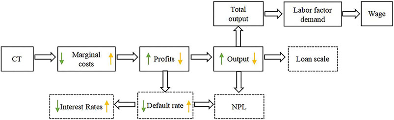
FIGURE 1. The transmission channel of CT. Note: The green arrow represents non-polluting enterprises, while the yellow arrow represents polluting enterprises. Dotted line boxes represent the effects of a CT on the banking sector, while straight line boxes represent implications for the real economy.

Furthermore, the effects of a CT on real economy and families are likely to have implications for financial stability via the banking sector. The implementation of a CT is anticipated to result in an increase in loan interest rates for PEs and a decrease in loan interest rates for NPEs. This, in turn, is expected to have an effect on the overall level of bank loan interest rates. The non-performing loan (NPL) ratio of banks is contingent upon both the magnitude of bank loans and the default risk of enterprises. The implementation of a CT has resulted in a rise in the default rate of PEs, a decline in the default rate of NPEs, and an alteration in the overall default rate of the community, ultimately impacting the NPL ratio of financial institutions. The capital adequacy ratio (CAR) of a bank is contingent upon its internal capital, loan portfolio size, and the risk weight of its loans. The implementation of a CT is expected to have an impact on the capital and loan scale of the concerned entity, which in turn may affect the CAR of the bank.

The implementation of a GSF reduces the risk weight of loans to NPEs, as the loan scale of banks is constrained by the minimum CAR, which in turn leads to the fact that banks can increase their loan size while holding the same amount of their own capital. Specifically, on the premise of meeting the minimum CAR requirement, banks will lower the interest rate of loans to non-polluting enterprises and expand the scale of loans to non-polluting enterprises.

The GSF affects the real sector of the economy through bank credit (Figure 2). For NPEs, a decreasing interest rate reduces the cost of financing, and the marginal cost of the firm’s product. For PEs, this effect does not exist. As a result, the profits of NPEs increase while those of PEs decrease in the product market. The interest rate of PEs rises accordingly.

FIGURE 2

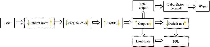
FIGURE 2. The transmission channel of GSF. Note: The green arrow represents non-polluting enterprises, while the yellow arrow represents polluting enterprises. Dotted line boxes represent the effects of a GSF on the banking sector, while straight line boxes represent implications for the real economy.

In addition, the implementation of a GSF leads to an increase in the output of NPEs and a decrease in the output of PEs. This, in turn, causes shifts in total social output and the total social demand for labor, ultimately influencing the wage level. For the household sector, the change in wage level affects the labor cost of the enterprise sector as well as the purchase demand for products. Following the discussion of risk transition path of a CT and a GSF, we build an improved DSGE model incorporating the banking sector in the next section.

After analyzing the shock transmission channel, we then consider the optimization behavior of household utility maximization, enterprise profit maximization, bank self-owned capital maximization, and government decision-making optimization, achieving partial equilibrium in different markets of the economic system to reach the final overall general equilibrium. The structure of the DSGE model with a CT and GSF is shown in Figure 3.

FIGURE 3

FIGURE 3. The structure of DSGE model with carbon tax (CT) and green supporting factor (GSF).

3.1 Model overview

3.1.1 Households

Assuming that there are a large number of homogeneous and infinitely resident households in the economy, a representative household maximizes the sum of its inter-temporal utility through inter-temporal consumption allocation, current labor supply, money and bond holdings. The utility function can be expressed as follows:

$E_t{\sum }_{t=0}^{\infty }{\beta }^t\left[\frac{{\left(C_t-{\varnothing }_c{C}_{t-1}\right)}^{1-\sigma }}{1-\sigma }-\frac{L_t^{1+\phi }}{1+\phi }+\frac{M_t^{1-\vartheta }}{1-\vartheta }\right](1)$

where $E_t$ is the expectation operator, β is the discount factor (0 < β < 1). $C_t$, $L_t$ and $M_t$ respectively represent the consumption, labor supply and household money holdings in period t. $\sigma$, $\phi$, $\vartheta$ respectively is the intertemporal elasticity of household consumption, the inverse of the labor supply, and the inverse of the elasticity of substitution of real money holdings. ${\varphi }_c$ is the habit parameter of household.

In this paper, we assume that the representative household earns interest income through savings and bond purchases in period t, in addition to obtaining labor wages. The constraint for the household is Eq. 2.

$P_t{C}_t+M_t+B_t+S_t=W_t{L}_t+\left(1+R_{t-1}\right)B_{t-1}+\left(1+r_{t-1}\right)S_{t-1}(2)$

where $P_t$ is the price of consumer goods, $B_t$ is the number of bonds held by the household, $W_t$ is the wage, $S_t$ is the household savings, $R_t$ and $r_t$ is the bond return and deposit interest rate respectively, and the new household deposit savings for each year is satisfied as:

$S_t=S_{t-1}+I_t(3)$

The first-order conditions for maximizing the representative household’s utility are

${\left(C_t-{\varnothing }_t{C}_{t-1}\right)}^{-\sigma }-{\varnothing }_c\beta E_t{\left(C_{t+1}-{\varnothing }_c{C}_t\right)}^{-\sigma }={\lambda }_t{P}_t(4)$

$-L_t^{\phi }={\lambda }_t{W}_t(5)$

$-M_t^{-\vartheta }={\lambda }_t(6)$

$E_t\left[{\lambda }_{t+1}\left(1+R_t\right)\right]={\lambda }_t(7)$

$E_t\left[{\lambda }_{t+1}\left(1+r_t\right)\right]={\lambda }_t(8)$

where ${\lambda }_t$ devotes the Lagrange multiplier.

3.1.2 Enterprises

We investigate the economic performance of enterprises under different climate change strategies, and observe variations in their responses. The enterprise sector is categorized into two groups, namely, PEs and NPEs. The following Cobb-Douglas function is utilized as the production function for a typical polluting enterprise.

$Y_{1,t}=A_{1,t}{L}_{1,t}^{\alpha }{K}_{1,t}^{1-\alpha }(9)$

where $Y_{1,t}$ is the output of the polluting enterprise and $L_{1,t}$, $K_{1,t}$ are labor employment level and capital in period t. The labor and capital output elasticity are devoted by α and 1-α, respectively. $A_{1,t}$ is the exogenous technology level of the polluting enterprise in period t, and obeys the logarithmic first-order autoregressive (i.e., AR(1)) process.

$\mathit{log}{A}_{1,t}={\rho }_A\mathit{log}{A}_{1,t-1}+{\epsilon }_{A_{1,t}},{\epsilon }_{A_{1,t}}\sim i.i.d.(10)$

where ${\rho }_A$ is the AR(1) coefficient of technology level.

At the end of period t-1, the decision of the polluting enterprise can be expressed as:

$K_{1,t}=\left(1-\delta \right)K_{1,t-1}+I_{1,t}\left[1-\frac{\chi }{2}{\left(\frac{I_{1,t}}{I_{1,t-1}}-1\right)}^2\right](11)$

where $\delta$ is the capital depreciation rate, $\mathrm{\chi }$ is the extent of change in investment adjustment costs. $I_{1,t}$ and $\frac{\chi }{2}{\left(\frac{I_{1,t}}{I_{1,t-1}}-1\right)}^2$ are respectively the new investment and investment adjustment cost of polluting enterprise $.$

This paper refers to Cao et al. (2021) for imposing a carbon tax on production, as it is more beneficial to control carbon emissions by taxing the production process. Assume that the carbon tax rate is an exogenous variable ${\tau }_{1,t}$, and obeys the following process.

$\mathit{log}{\tau }_{1,t}=\left(1-{\rho }_t\right)\mathit{log}\overline{{\tau }_{1,t}}+{\rho }_t\mathit{log}{\tau }_{1,t-1}+{\epsilon }_{{\tau }_{1,t}},{\epsilon }_{{\tau }_{1,t}}\sim i.i.d.(12)$

where ${\rho }_{\tau }$ is the AR(1) coefficient of the carbon tax rate $.$

Eq. 13 can be used to describe the polluting enterprise’s profit-maximization behaviors:

${\mathit{max}}_{\left\{L_{1,t},K_{1,t}\right\}}{E}_t\prod =P_t{Y}_{1,t}-\left[W_t{L}_{1,t}+r_{1,t}{K}_{1,t}+{\tau }_{1,t}{CE}_t\right](13)$

where $r_{1,t}$ is the loan interest rate of the polluting enterprise. ${CE}_t$ denotes the carbon emissions, affected by the level of output of polluting enterprise and the level of environmental protection technology, the specific expression can be written as:

${CE}_t=l{Y}_{1,t}{ET}_t^{-1}(14)$

where $l$ is the carbon emission intensity based on output. ${ET}_t$ is the level of environmental technology, and it is assumed to obey the following process.

$\mathit{log}{ET}_t=\left(1-{\rho }_{ET}\right)\bullet \mathit{log}\overline{{ET}_t}+{\rho }_{ET}\mathit{log}{ET}_{t-1}+{\epsilon }_{{ET}_t},{\epsilon }_{{ET}_t}\sim i.i.d.(15)$

where ${\rho }_{ET}$ is the AR(1) coefficient of environmental technology $.$

The first-order conditions for maximizing polluting enterprise’s profits are

$\frac{\alpha P_t}{L_{1,t}}\bullet Y_{1,t}-W_t-\frac{l{\tau }_{1,t}{Y}_{1,t}{ET}_t^{-1}\alpha }{L_{1,t}}=0(16)$

$\frac{\left(1-\alpha \right)P_t}{K_{1,t}}\bullet Y_{1,t}-r_{1,t}-\frac{l{\tau }_{1,t}{Y}_{1,t}{ET}_t^{-1}\left(1-\alpha \right)}{K_{1,t}}=0(17)$

It is further considered that the probability of default on corporate loans increases when the production and operation of polluting enterprise are unstable. This paper refers to Dunz et al. (2021), assuming that the default rate of polluting enterprise is

$c_{1,t}=c_{1,t-1}\bullet \left(1-\frac{{\pi }_{1,t}-{\pi }_{1,t-1}}{{\pi }_{1,t-1}}\right)(18)$

The default scale of polluting enterprise is

${NPL}_{1,t}=c_{1,t}{K}_{1,t}(19)$

The production function of a representative non-polluting enterprise is

$Y_{2,t}=A_{2,t}{L}_{2,t}^{\alpha }{K}_{2,t}^{1-\alpha }(20)$

where $Y_{2,t}$ is the output of non-polluting enterprise and $L_{2,t}$, $K_{2,t}$ are respectively labor employment level and capital in period t. The labor and capital output elasticity are denoted by α and 1-α, respectively. $A_{2,t}$ is the exogenous technology level of the non-polluting enterprise in period t, and obeys the logarithmic first-order autoregressive process.

$\mathit{log}{A}_{2,t}={\rho }_A\mathit{log}{A}_{2,t-1}+{\epsilon }_{A_{2,t}},{\epsilon }_{A_{2,t}}\sim i.i.d.(21)$

where ${\rho }_A$ is the coefficient of technology level $.$

At the end of period t-1, the decision of the non-polluting enterprise can be expressed as:

$K_{2,t}=\left(1-\delta \right)K_{2,t-1}+I_{2,t}\left[1-\frac{\chi }{2}{\left(\frac{I_{2,t}}{I_{2,t-1}}-1\right)}^2\right](22)$

where $I_{2,t}$ and $\frac{\chi }{2}{\left(\frac{I_{2,t}}{I_{2,t-1}}-1\right)}^2$ are respectively the new investment and investment adjustment cost of non-polluting enterprise $.$

Eq. 23 can be used to describe the non-polluting enterprise’s profit-maximization behaviors:

${\mathit{max}}_{\left\{L_{2,t},K_{2,t}\right\}}{E}_t{\prod =P}_t{Y}_{2,t}-\left[W_t{L}_{2,t}+r_{2,t}{K}_{2,t}\right](23)$

where $r_{2,t}$ is the loan interest rate of the non-polluting enterprise.

The first-order condition for maximizing non-polluting enterprise’s profits are

$\frac{\alpha Y_{2,t}}{L_{2,t}}=W_t(24)$

$\frac{\left(1-\alpha \right)Y_{2,t}}{L_{2,t}}=r_{2,t}(25)$

We assume that the default rate of non-polluting enterprise is

$c_{2,t}=c_{2,t-1}\left(1-\frac{{\pi }_{2,t}-{\pi }_{2,t-1}}{{\pi }_{2,t-1}}\right)(26)$

The default size for the non-polluting enterprise is

${NPL}_{2,t}=c_{2,t}{K}_{2,t}(27)$

In a market economy, there is incomplete and untimely adjustment of market prices, which causes sticky prices. When the products of both types of firms enter the final consumer market, the total social output can be represented by a constant elasticity of substitution production function, which is as follows:

$Y_t={\left[\gamma Y_{1,t}^{1-\mu }+\left(1-\gamma \right)Y_{2,t}^{1-\mu }\right]}^{\frac{1}{1-\mu }}(28)$

where $\gamma$ denotes the weight on polluting enterprises’ output in the total output, and µ denotes the elasticity of substitution between output of polluting and non-polluting enterprises.

Similarly, the total marginal cost of the two firms is:

${MC}_t={\left[{\gamma }_m{MC}_{1,t}^{1-{\mu }_m}+\left(1-{\gamma }_m\right){MC}_{2,t}^{1-{\mu }_m}\right]}^{\frac{1}{1-{\mu }_m}}(29)$

So, for each firm j, its maximized return can be expressed as:

$\underset{P_{j,t}^{*}}{\max }{E}_t{\sum }_{j=0}^{\infty }\left[{{\beta }_{\theta }}^j(P_{j,t}^{*}{Y}_{j,t+i}-{MC}_{j,t+i}\right.Y_{j,t+i}\left)\right](30)$

From Eq. 30, its first-order condition can be obtained as:

$Y_{j,t}=Y_t{\left(\frac{P_t}{P_{j,t}}\right)}^{\mu }(31)$

From Eqs 30, 31, this paper obtains

$\underset{P_{j,t}^{*}}{\max }{E}_t{\sum }_{j=0}^{\infty }\left\{{{\beta }_{\theta }}^j[P_{j,t}^{*}{Y}_{j,t+i}{\left(\frac{P_{t+i}}{P_{j,t}}\right)}^{\mu }-Y_{j,t+i}{\left(\frac{P_{t+i}}{P_{j,t}}\right)}^{\mu }\right.{MC}_{j,t+i}\left]\right\}(32)$

The first-order derivative of Eq. 32 is

$P_{j,t}^{*}=\left(\frac{\mu }{\mu -1}\right)E_t{\sum }_{j=0}^{\infty }\left({{\beta }_{\theta }}^i{MC}_{j,t+i}\right)(33)$

Thus, the final market price can be expressed as follows:

${\mathrm{P}}_{\mathrm{t}}={\left[\mathrm{\mu }{\mathrm{P}}_{\mathrm{t}-1}^{1-\mathrm{\mu }}+{\left(1-\mathrm{\mu }\right)\mathrm{P}}_{\mathrm{t}}^{1-\mathrm{\mu }}\right]}^{\frac{1}{1-\mathrm{\mu }}}(34)$

3.1.3 Banking sector

We adopt the form of Gerali et al. (2010) to set the banking sector. Assuming that commercial banks are in a perfectly competitive market and their business consists of deposits and loans, the accounting equilibrium equation for commercial banks can be written as:

$K_{1,t}+K_{2,t}=S_t+B_t+N_t(35)$

where $K_{1,t}+K_{2,t}$ is the banking sector’s total loans (i.e., the banking sector’s total assets), $S_t+B_t$ denotes the banking sector’s total deposits taken (i.e., the banking sector’s total liabilities), and $N_t$ represents the banking sector’s own capital (i.e., the owner’s equity in banks). Referring to Dunz et al. (2021), this paper assumes that a banking sector’s own capital consists of the sum of accumulated capital in the previous period and operating profit in the current period, which can be expressed as:

$N_t=\left(1-n\right)N_{t-1}+J_t(36)$

where n is the resources used up in managing bank capital and $J_t$ is the operating profit of the banking sector in period t. The profits are influenced by market business returns on the one hand, and by policy regulation, which imposes fines on banks, on the other. Consequently, the precise expression of $J_t$ is as follows:

$J_t=r_{1,t}{K}_{1,t}+r_{2,t}{K}_{2,t}-r_t{S}_t-R_t{B}_t-\frac{p}{2}{\left({CAR}_t-\overline{\left.CAR\right)}\right.}^2{N}_t(37)$

${CAR}_t=\frac{N_t}{k_{1,t}{K}_{1,t}+k_{2,t}{K}_{2,t}}(38)$

where $r_{1,t}{K}_{1,t}$ and $r_{2,t}{K}_{2,t}$ are the interest income from loans to polluting and non-polluting by the banking sector in period t, respectively, and $r_t{S}_t$ and $R_t{B}_t$ are the expenses of the banking sector in paying interest on deposits and interest on bonds in period t. $\frac{p}{2}{\left({CAR}_t-\overline{\left.CAR\right)}\right.}^2{N}_t$ represents the penalty given when the CAR of the banking sector deviates from the minimum CAR required by the regulator, and $p$ is the penalty intensity induced by deviations from capital adequacy targets in the banking sector. $k_{1,t}$ and $k_{2,t}$ are risk weights of loans to polluting and non-polluting enterprise.

When the GSF is introduced, $k_{2,t}$ can be expressed as:

$\mathit{log}{k}_{2,t}=\left(1-{\rho }_{k_2}\right)\mathit{log}\overline{k_{2,t}}+{\rho }_{k_2}\mathit{log}{k}_{2,t-1}+{\epsilon }_{k_{2,t}},{\epsilon }_{k_{2,t}}\sim i.i.d.(39)$

where ${\rho }_{k_2}$ is the AR(1) coefficient for the risk weight of non-polluting enterprise $.$

Referring to Dunz et al. (2021), the expression for the interest rate on corporate loans in the banking sector is as follows:

$r_{1,t}=r_0+a\frac{{NPL}_{1,t}}{K_{1,t}}+b_1\left(k_{2,t}-k_1\right)(40)$

$r_{2,t}=r_0+a\frac{{NPL}_{2,t}}{K_{2,t}}+b_2\left(k_{2,t}-k_1\right)(41)$

where $r_0$ is the base interest, ${NPL}_{1,t}$, ${NPL}_{2,t}$ are the default amounts of polluting and NPEs, respectively, a is the sectoral interest rate adjustment rate, $b_1$, $b_2$ are the GSF interest rate adjustment rate of PEs and NPEs, respectively.

The banking sector’s own capital optimization problem can be expressed as:

$\max E_t\prod =\left(1-n\right)N_{t-1}+r_{1,t}{K}_{1,t}+r_{2,t}{K}_{2,t}-r_t{S}_t-R_t{B}_t-\frac{p}{2}{\left({CAR}_t-\overline{\left.CAR\right)}\right.}^2{N}_t(42)$

The first-order condition of Eq. 42 can be obtained by constructing the Lagrangian function as:

$\mathrm{\Lambda }\left(1-n\right)-\frac{p}{2}{\left({CAR}_t-\overline{\left.CAR\right)}\right.}^2-p{CAR}_t\left({CAR}_t-\overline{CAR}\right)=0(43)$

$r_t=Q_t(44)$

$R_t=Q_t(45)$

${-r}_{1,t}=Q_t(46)$

${-r}_{2,t}=Q_t(47)$

where $Q_t$ is the Lagrangian multiplier.

3.1.4 Government

Suppose the government only engages in taxation and expenditure, and that there are neither fiscal deficits nor surpluses. Government’s budget constraint in time t can be formulated as follows:

$G_t={\tau }_{1,t}{CE}_t(48)$

where $G_t$ is the government expenditure in period t and ${\tau }_{1,t}{CE}_t$ is the tax collected from the polluting enterprise emitting CO₂ as their revenue.

The government applies a price-based monetary policy using Taylor’s rule, namely,

$\frac{r_t}{\overline{r}}={\left(\frac{r_{t-1}}{\overline{r}}\right)}^{{\theta }_r}{\left[{\left(\frac{{\pi }_t}{\overline{\pi }}\right)}^{{\phi }_{\pi r}}{\left(\frac{Y_t}{\overline{Y}}\right)}^{{\phi }_{Yr}}\right]}^{1-{\theta }_r}\bullet {\epsilon }_{rt},{\epsilon }_{rt}\sim i.i.d.(49)$

where ${\theta }_r$ is the savings rate smoothing coefficient, ${\phi }_{\pi r}$ and ${\phi }_{Yr}$ are the inflation rate response coefficient and the output rate response coefficient, respectively. $\overline{\pi },\overline{\mathrm{Y}}$ and $\overline{r}$ are the equilibrium levels of inflation, output, and saving rate.

3.1.5 Market clearing

The conditions of market-clearing of both labor market and capital market are listed in Eqs 50, 51, for which the supply meets the demand.

$L_t=L_{1,t}+L_{2,t}(50)$

$I_t=I_{1,t}+I_{2,t}(51)$

According to Walrasian general equilibrium theory, the market-clearing condition is

${\mathrm{Y}}_{\mathrm{t}}={\mathrm{C}}_{\mathrm{t}}+{\mathrm{I}}_{\mathrm{t}}+{\mathrm{G}}_{\mathrm{t}}(52)$

3.2 Parameter calibration and estimation

In order to solve the model, static parameters values need to be assigned. This study calibrates these values by referring to previous literature and real economic data. The values of these parameters are presented in Table 1. The robustness of the model was assessed by systematically varying each parameter within a tolerable range. There were no significant alterations in the outcomes. This demonstrates the resilience and reliability of the model. In addition, the estimation of dynamic parameters is realized by Bayesian estimation using GDP of China from 2000 to 2020 as the real variables (Table 2), refering to Amiri et al. (2021), Cao et al. (2021), and Liu and He (2021). And we set the autoregressive coefficients of the exogenous shock variables to a normal distribution and the random disturbance terms to an Inv-Gamma distribution, referring to Smets and Wouters (2007). The GDP data are obtained from the National Bureau of Statistics of China.

TABLE 1

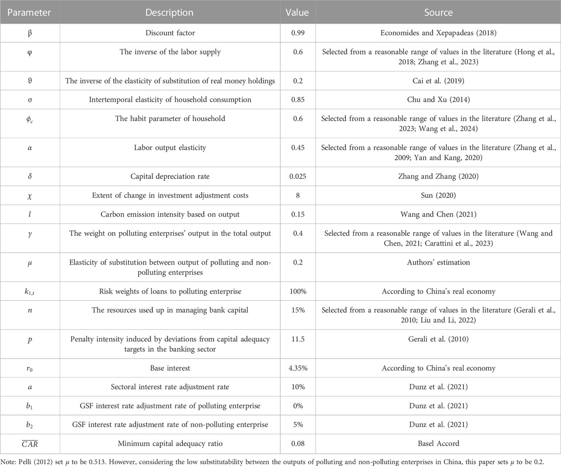
TABLE 1. Steady-state parameters calibration.

TABLE 2

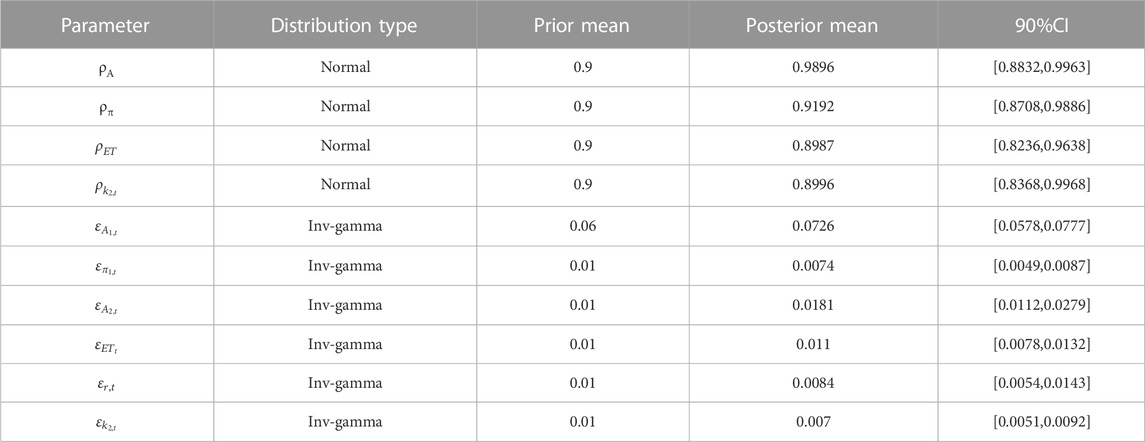
TABLE 2. Bayesian estimation results.

4 Empirical results and discussion

The improved DSGE model can be used for policy simulation and scenario analysis with the parameters. The model is first maintained at the steady-state level in the following sections, after which an exogenous policy shock is administered to the model and the impulse response curves of each variable to the policy shock are obtained. We assume three policy shock strengths of 1%, 5%, and 10%, respectively. In Section 4.1 and Section 4.2, we simulate the impact of the carbon tax and the green supporting factor shocks, and in Section 4.3, we compare and explain the simulation results. The economic system’s impulse reaction curves to the carbon tax shock are shown in Figures 4, 5, while the financial stability’s impulse response curves to the green supporting factor shock are shown in Figures 6, 7, respectively. The horizontal axis indicates the lag period of the shock (100-quarter) and the vertical axis indicates the deviation of the variable from the steady-state value. The solid line indicates a 1% shock, the dashed line indicates a 5% shock, and the dotted line indicates a 10% shock.

FIGURE 4

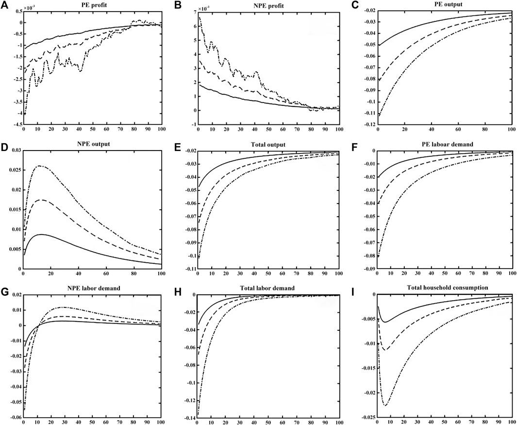
FIGURE 4. Impulse response of a carbon tax to the economic system. (A) PE profit, (B) NPE profit, (C) PE output, (D) NPE output, (E) Total output, (F) PE labor demand, (G) NPE labor demand, (H) Total labor demand, (I) Total household consumption.

FIGURE 5

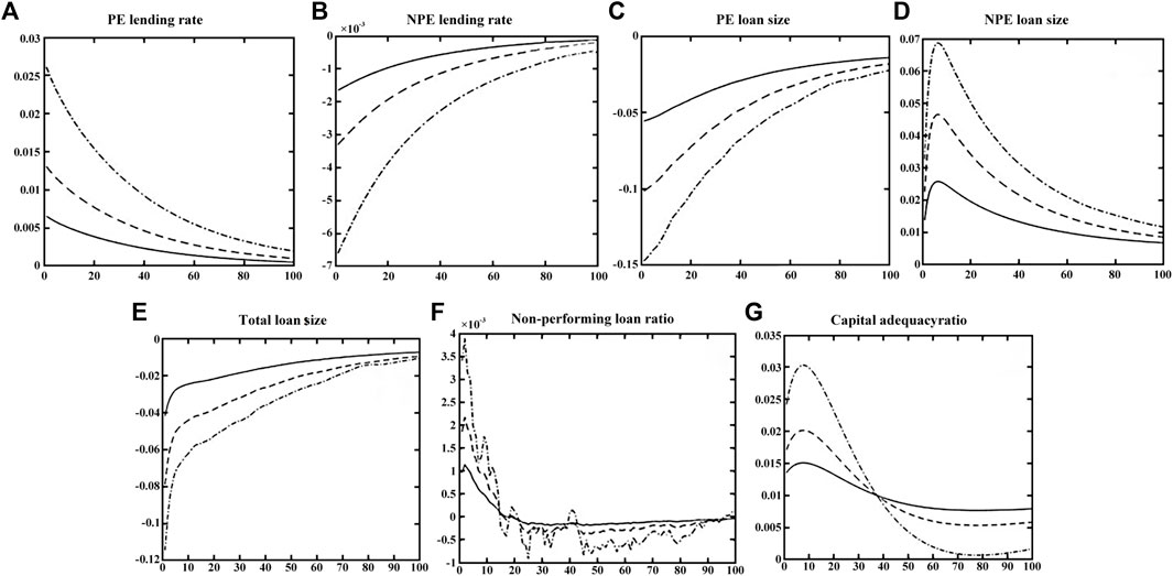
FIGURE 5. Impulse response of a carbon tax to the economic system. (A) PE lending rate, (B) NPE lending rate, (C) PE loan size, (D) NPE loan size, (E) Total loan size, (F) Non-performing loan ratio, (G) Capital adequacy ratio.

FIGURE 6

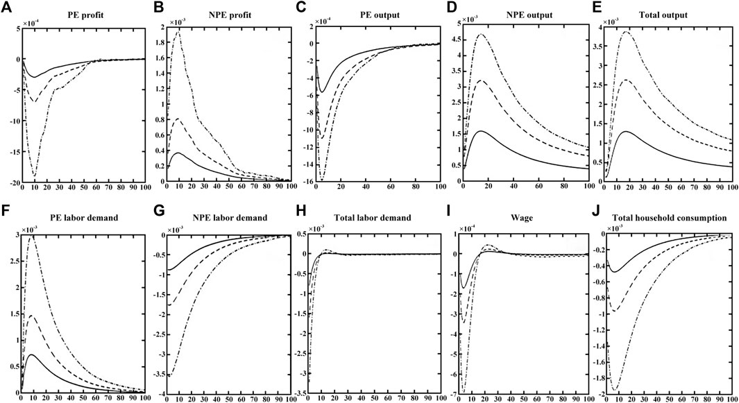
FIGURE 6. Impulse response of a carbon tax to the economic system. (A) PE profit, (B) NPE profit, (C) PE output, (D) NPE output, (E) Total output, (F) PE labor demand, (G) NPE labor demand, (H) Total labor demand, (I) Wage, (J) Total household consumption.

FIGURE 7

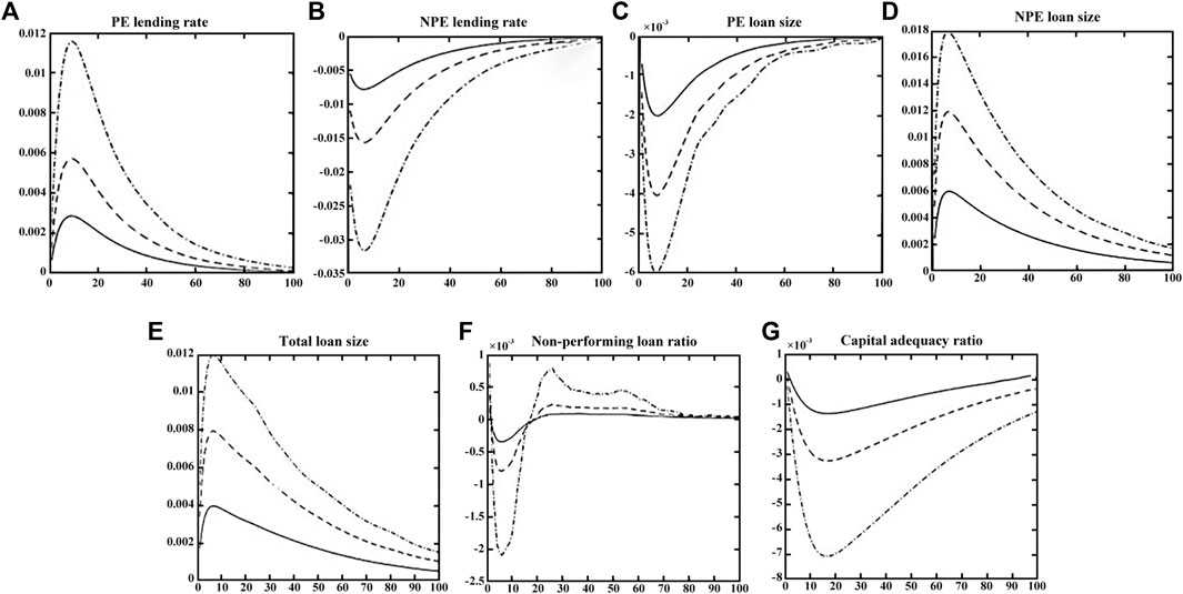
FIGURE 7. Impulse response of a carbon tax to the economic system. (A) PE lending rate, (B) NPE lending rate, (C) PE loan size, (D) NPE loan size, (E) Total loan size, (F) Non-performing loan ratio, (G) Capital adequacy ratio.

4.1 The impulse-response functions to carbon tax

4.1.1 Impulse response analysis of the economic system to the carbon tax

(1) Impulse response analysis of corporate profits to the carbon tax

The impulse responses of the economic system to carbon tax shocks are shown in Figure 4. Following a positive carbon tax shock, PEs will see a decline in profit, while NPEs will see an increase. The possible explanation is that when the carbon tax rate rises for PEs, the marginal cost of PEs rises in the short run. And market prices remain essentially unchanged in the short run, so the profits of PEs fall and the profits of NPEs rise. However, both types of businesses will reach the steady-state value in the long run. As the impact of carbon tax policy becomes more pronounced, corporate profit is likely to become increasingly unstable. The deviation may be attributed to the impact of tax disturbance on market equilibrium. Furthermore, a 1% carbon tax shock will result in a maximum 0.12% deviation from the steady-state value for PEs, while the figure of NPEs is 0.19%.

(2) Impulse response analysis on corporate output to the carbon tax

As shown in Figure 4, with implementation of a carbon tax policy, PEs are expected to experience an initial adverse impact on their output, which is anticipated to diminish over successive simulation periods. In the long term, the output of these enterprises is expected to remain below the initial equilibrium level. In the short term, the production of NPEs is expected to increase initially and subsequently decrease, while remaining above the initial equilibrium level for an extended period. The maximum negative deviation of the output of PEs varies across different levels of policy impact. As the carbon tax policy’s impact intensifies, PEs’ output level will experience a peak negative deviation ranging from 5.1% to 11.2%, and a long-term negative deviation ranging from 2.1% to 2.8%. The findings suggest that NPEs exhibit a peak positive deviation ranging from 0.8% to 2.6% under varying intensity shock levels during the 10th phase. In the long run, a new equilibrium is established, characterized by a positive deviation range of 0.2%–0.4%.

Next, we consider the distinct consequences of a carbon tax shock to the total output of society. On the one hand, lower profits for PEs lead them to lower output, with a negative impact on total output. On the other hand, rising profits of NPEs lead to an increase in output, with a positive impact on total output. Overall, the carbon tax has a far greater negative impact on the production of PEs than it does on NPEs. The trend of total social output is essentially the same as that of PEs, as can also be observed in Figure 4. In particular, after a carbon tax shock, the overall social output will fall, and will ultimately be less than the steady-state value.

(3) Impulse response analysis of labor demand to the carbon tax

As shown in Figure 4, in the short run, carbon tax policy reduces PEs’ labor demand while increasing NPEs’. In the long term, the carbon tax policy will have a diminishing effect on the labor demand of the two types of businesses. When the carbon tax policy impact increases from 1% to 10%, PEs experience an immediate negative response in labor demand ranging from 2.1% to 8%. However, this effect gradually diminishes over time and eventually stabilizes slightly below the initial level. In contrast, NPEs experience an immediate reduction ranging from 1.5% to 5.5% as the intensity of the carbon tax policy impact increases, within the first 20 simulation periods. Following the 20th period, the upward shift in labor demand for NPEs will escalate in proportion to the degree of policy impact intensity. However, it will ultimately surpass the initial equilibrium level only by a marginal amount. In terms of response peak and ultimate equilibrium deviation, the labor demand of PEs is more significantly affected by the implementation of a carbon tax policy compared to NPEs.

Further considering the impact of the carbon tax shock on the total labor demand. Figure 4 shows that the carbon tax policy initially decreases the labor demand of both PEs and NPEs, resulting in a 3.6%–13.5% decrease in total social labor demand. In the long term, the total social labor demand returns to the steady-state value. After a carbon tax shock, the PEs scale down their production to reduce carbon emissions, and their labor demand drops. In contrast, expansion of output by NPEs increases the demand for labor factors. However, when the policy was first put into effect, NPEs experienced a short-term negative reaction to labor demand. This is mainly because the implementation of a carbon tax policy leads to increased profits for NPEs (Figure 4), which in turn increases their solvency, and banks tend to lower the interest rates on loans provided to these enterprises, thereby reducing the cost of capital. Consequently, NPEs experience an increased demand for capital factors and a decreased demand for labor factors. However, with the long-term adjustment of capital factor and labor factor price, the final steady-state value of labor demand will revert to its initial value.

(4) Impulse response analysis of household sector consumption to the carbon tax

As shown in Figure 4, when the intensity of carbon tax policy increases from 1% to 10%, household consumption will have an instantaneous negative response of 0.25%–1% and attain a maximum negative deviation of 0.5%–2.3% in the ninth phase, which is less than the initial steady-state value in the long run. In addition, the household sector’s consumption level will decline in the short run, but the declining state will not last for a long time. The specific reason is that after the implementation of the carbon tax policy, the market demand for labor factors will gradually recover (Figure 4), and the wage level will gradually rise, which in turn will lead to a subsequent recovery of the household consumption level. In the long term, however, the consumption level of the household sector after the impact of the carbon tax policy is still lower than the initial constant value. This is due to the crowding-out effect of the tax policy, which reduces the family’s standard of living.

4.1.2 Impulse response analysis of the financial stability to the carbon tax

(1) Impulse response analysis of bank sector lending rates to the carbon tax

Figure 5 demonstrates the impulse responses of the financial system to the carbon tax shock. For NPEs, the impact of carbon tax policy on their loan interest rate is negative. Under the impact intensity of 1%–10%, the loan interest rate will deviate negatively by 0.18%–0.67%. The effect of the carbon tax policy on the loan interest rate of PEs is positive, and significantly greater than that of NPEs. Under the same level of carbon tax, the absolute deviation range of loan interest rates for PEs is approximately three times that of NPEs. The influence of carbon tax policy on the loan interest rate of two types of businesses decreases progressively as the simulation period lengthens. Long-term, however, as a result of the carbon tax policy, the loan interest rate for PEs will be higher than the original steady-state value, while that for NPEs will be lower. In general, the impact of carbon tax policy on the loan interest rate of PEs is greater than that of NPEs.

The implementation of a carbon tax policy results in a reduction in profits for PEs, increases the default risk, and causes a corresponding rise in loan interest rates from the banking sector to such enterprises. The increase in profitability of NPEs is expected to coincide with a reduction in the default risk of such enterprises. This trend is likely to prompt a decrease in the interest rate extended to NPEs by the banking sector. Generally speaking, a carbon tax policy results in a greater increase in the interest rates extended to PEs compared to the decrease in interest rates to NPEs. Consequently, it results in an elevation of the interest rate associated with bank loans, thereby promoting financial stability.

(2) Impulse response analysis of loan size of bank sector to the carbon tax

As shown in Figure 5, following a carbon tax shock, the deviation of loan size is negative for PEs. It decays as the number of simulation periods increases, and their output will be lower than the steady-state value in the long term. The loan size of NPEs will respond positively to the impact of carbon tax policy and will deviate positively from the original steady-state value in the long term. At the time of policy implementation, PEs will have a negative deviation peak between 5.5% and 14.9%, while NPEs will have a positive deviation peak between 2.6% and 6.9%. This demonstrates the asymmetric effect of the carbon tax on loan size for both types of enterprises, with a greater impact on PEs.

PEs’ default rate may rise as a result of their declining profitability once the carbon tax policy is in effect. As a result, the banking industry might increase its interest rate on these businesses in response, causing PEs to reduce their borrowing. Meanwhile, the rise in profits observed among the NPEs will lead to a corresponding decline in their default rate. The banking sector will reduce the lending rate applicable to these enterprises. This, in turn, encourages NPEs to increase their borrowing. Overall, the implementation of a CT generally leads to a reduction in the lending size of banks, so contributing to an increase in financial stability.

(3) Impulse response analysis of the non-performing loan (NPL) ratio of the banking sector to the carbon tax

As shown in Figure 5, in the short term, the NPL ratio of the banking sector is positively affected by a carbon tax policy, but in the long term, it is insignificant. The larger the impact of the carbon tax policy, the greater the fluctuations in the nonperforming loan ratio. As the impact of policy intensity increases, the profit deviation amplitude of the enterprise sector will fluctuate more, and the corporate default rate will be affected by its own profit variations, causing the bank’s NPL ratio to fluctuate more as well. In addition, when the impact of carbon tax policy increases from 1% to 5%, the NPL ratio of banks will immediately generate a positive deviation of 0.1%–0.18%, but the positive response gradually declines and returns to the initial equilibrium after the 20th period. However, when the impact of carbon tax policy is 10%, the NPL ratio of banks will generate a positive deviation of 0.34%, and a negative deviation within the range of 0%–0.1% will persist after the 20th period.

After the implementation of a carbon tax policy, it will initially have a direct impact on the profits and default risk of polluter enterprises, and an increase in the NPL ratio of banks. However, as time passes, the influence of carbon tax policy on the NPL ratio will quickly revert to its initial equilibrium value by adjusting the ratio of loans to NPEs to loans to PEs, as well as by enterprises adjusting their own business conditions. In general, a carbon tax policy would have negative short-term effects on financial stability, but these effects would diminish over time.

(4) Impulse response analysis of the banking sector’s capital adequacy ratio (CAR) to the carbon tax

As shown in Figure 5, following the carbon tax shock, the deviation of CAR is positive, and stays at a higher level than the steady-state value in the long term. The level of CAR in the banking sector will climax in the 10th phase, with positive deviations ranging from 1.5% to 3%. A new equilibrium is attained over time, with a positive deviation ranging from 0.2% to 0.7%. However, the degree of deviation from the CAR increases with increasing policy intensity shocks until the 39th quarter and decreases with increasing policy shocks after the 39th quarter.

The CAR is influenced by a bank’s capital and loan size. Consequently, after the implementation of a carbon tax policy, the decrease in bank loan size will result in an increase in CAR. However, the decrease in loan size will also be accompanied by a decrease in bank profits, which in turn causes a decrease in the bank’s own capital. Prior to the 10th period, the rate of decline of the bank’s own capital is slower than that of the bank’s loan scale, causing the CAR to increase. After attaining the peak of positive deviation in the 10th phase, the CAR shows a gradual decline, but remained above the initial steady-state value. In general, the policy regarding the carbon tax will increase banks’ CAR, thereby enhancing financial stability.

4.2 The impulse-response functions to a green supporting factor

4.2.1 Impulse response analysis of the economic system to the green supporting factor

(1) Impulse response analysis of corporate sector profit to the green supporting factor

As shown in Figure 6, following a green supporting factor shock, the deviation of profit is negative for PEs and positive for NPEs in the short term, but profits of both types of enterprises will reach the steady-state value in the long term. Specifically, PEs generate negative deviation peaks ranging from 0.03% to 0.19%, whereas NPEs maintain deviations ranging from 0.04% to 0.19%. Under the same impact intensity of the green supporting factor policy, both types deviate from the peak value at the same time and remain at approximately the 10th stage under various impact intensities. Figure 6 also demonstrates that the profit change of PEs initially decreases, then increases, and eventually returns to its initial equilibrium level, while for NPEs, some of the effects will be delayed, but in the long term, the profits of NPEs will return to their initial steady-state value.

The green supporting factor will directly affect the loan interest rate of NPEs, which will lead to the decrease of capital factor price and the marginal cost of enterprises. Therefore, the profit of NPEs rises. In contrast, PEs are unable to adjust in time in the short term, resulting in their marginal costs being higher than the market price, which makes profits fall. However, in the long term, enterprises can adjust their factor input levels, and both types of enterprises’ profit deviations gradually return to their original steady-state values.

(2) Impulse response analysis of enterprise sector output to the green supporting factor

As shown in Figure 6, upon implementation of a green supporting factor policy, PEs’ output will experience a short-term decline followed by a subsequent rise, ultimately returning to their original steady-state value in the long term. The output of NPEs will experience an initial increase followed by a subsequent decrease, ultimately settling at a long-term equilibrium point higher than the initial steady-state value. As the green supporting factor policy impact rises from 1% to 10%, there is a negative deviation peak of the output of PEs, ranging from 0.05% to 0.16%. The reaction of NPEs is adverse, ranging from 0.16% to 0.47%. Overall, the impact of green supporting factor policy on the output of PEs is comparatively weaker than that on NPEs.

Further consider the impact of the green supporting factor shock on the total output of society. It is evident from Figure 6 that the impact can be segmented into two distinct phases. During the initial phase, the influence of the green supporting factor policy is more significant on NPEs. Consequently, the short-term response of the overall social output is generally in line with that of NPEs. In the long term, PEs’ output reverts to the steady state, whereas NPEs’ output surpasses the initial steady state. Consequently, the overall output of society slightly exceeds the initial equilibrium level.

(3) Impulse response analysis of enterprise sector labor demand to the green supporting factor

As shown in Figure 6, following a green supporting factor shock, there will be an initial increase in labor demand for PEs, followed by a subsequent decline in the short term. The peak of this trend is projected to occur during the 10th period. NPEs are expected to experience an immediate reduction in labor demand as a result of the implementation of a green supporting factor policy. However, over time, the labor demand is anticipated to gradually return to its original equilibrium level. As the magnitude of the green supporting factor policy intensifies from 1% to 10%, there is an increase in the favorable deviation of the labor demand of polluters from 0.07% to 0.3%. However, in the long term, the demand is expected to revert to its original stable level. The kurtosis of labor demand in NPEs has experienced an increase in negative deviation, rising from 0.08% to 0.35%. The observed shock response can be attributed to the impact of the green supporting factor policy on the capital price, which subsequently influences the demand for capital factors of the two types of enterprises.

Further consider the effect of a green supporting factor shock on total labor demand. It can be seen from Figure 6, the initial decline in labor demand for NPEs is greater than the rise for PEs. In the long term, the total social labor demand returns to its steady-state value.

(4) Impulse response analysis of household sector consumption to the green supporting factor

As shown in Figure 6, following the green supporting factor shock, the wage tends to fall and then rise in the short term, and returns to the steady-state value in the long term. When the green supporting factor policy impact increases from 1% to 10%, the wage level of the household sector will initially experience an instantaneous negative deviation of 0.01%–0.04%, reach a maximum negative deviation of 0.02%–0.07% in the fourth period.

Furthermore, the adoption of the green supporting factor policy will result in a short-term reduction in social labor demand. As the labor supply cannot be promptly adjusted, there will be a decrease in the price of labor factors and a subsequent reduction in family income, ultimately resulting in a decline in household consumption. Therefore, the household sector’s consumption level is generally consistent with the trend of wage levels, albeit exhibiting a slower decline compared to household wages.

4.2.2 Impulse response analysis of financial stability on green supporting factor

(1) Impulse response analysis of bank sector loan interest rates to the green supporting factor

As shown in Figure 7, following the green supporting factor shock, the loan interest rate of polluting businesses will rise initially, then reduce, and remain slightly above the steady level in the long run, while for NPEs. The deviation of bank sector loan interest rates is negative, and in the long term, interest rates will be lower than the steady-state value. The green supporting factor policy shock on NPEs is more severe than that on PEs.

From Eqs 40, 41, it is known that the interest rate of corporate loans is affected by the risk weight of enterprises and the default rate. Analyzing the above impulse response results, it can be seen that on the one hand, when the green supporting factor policy is implemented, the risk weight of NPEs decreases. On the other hand, from Figure 6, it is known that the profit of NPEs first rises and then falls, then the default first falls and then rises. Therefore, the implementation of green supporting factor policy will make the lending rate of NPEs fall first and then rise. On the contrary, for PEs, the profit of enterprises decreases and then increases, and defaults first rise and then fall, which leads to the increase and then decrease of loan interest rate. Typically, the implementation of a green supporting factor policy results in a greater reduction of loan interest rates for NPEs compared to the increase in interest rates for PEs. Hence, the implementation of a green supporting factor policy results in a reduction in the aggregate lending rate, which may not be favorable for maintaining financial stability.

(2) Impulse response analysis of bank sector loan size on the green supporting factor

As shown in Figure 7, green supporting factor policy has a negative effect on the loan scale of PEs, with a short-term trend of decreasing, followed by an increase, and a long-term return to the steady-state value. The loan scale of NPEs exhibits a positive response, with a short-term trend of first increasing and then decreasing, and a long-term trend of exceeding the initial stable level. When the impact intensity of the green supporting factor policy ranges from 1% to 10%, PEs produce a negative deviation peak in the range of 0.2%–0.6%, whereas NPEs produce a positive deviation peak in the range of 0.6%–1.8%. This indicates that the loan size effect of the two types of enterprises is asymmetrical, and that the green supporting factor policy has a greater impact on NPEs.

As shown in Figure 7, the implementation of a green supporting factor policy reduces the risk weight of NPEs, allowing banks with the same quantity of capital to extend more loans to these businesses. Long-term, green supporting factor policy will increase banks’ loan scale, thereby weakening the financial system’s stability.

(3) Impulse response analysis of bank sector non-performing loan (NPL) ratio to the green supporting factor.

As shown in Figure 7, following the introduction of the policy, the NPL ratio will immediately exhibit a positive effect, but in the short term, the overall trajectory will decline and then rise. Specifically, the fluctuation range of the NPL ratio increases proportionally as green supporting factor policy intensifies. The negative deviation degree of NPL ratio increased in the first 20 periods as green supporting factor policy intensity increased. However, after the 20th period, the increase in shock intensity led to a rise in the positive deviation degree of the NPL ratio. In the long run, the NPL ratio of banks will return to the original stable level.

As shown in Figure 7, the loan scale of NPEs increases and the default rate decreases in the short term following the implementation of a policy. Loans to polluting businesses have decreased, and default rates have increased. The proportion of total bank loans comprised of loans to PEs is small. As a consequence, the NPL ratio in the banking sector tends to decrease first. In the long term, however, the NPL ratio will revert to a stable level. In general, the green supporting factor policy will cause the NPLs of banks to decrease, then rise, and then revert to a stable level, thereby affecting the financial stability.

(4) Impulse response analysis of the banking sector’s capital adequacy ratio (CAR) on the green supporting factor

As shown in Figure 7, the CAR has an instantaneous weak positive effect on the green supporting factor policy, but the overall trend is to fall and then rise, and in the long term, CAR will be lower than the steady-state value. In particular, as the impact of policy intensity increases from 1% to 10%, the CAR of the banking sector will form a negative deviation peak between 0.12% and 0.7% in the 17th period, with the negative deviation remaining between 0% and 0.13% in the long term.

After the implementation of a green supporting factor policy, the risk weight of NPEs will diminish, and the CAR will rise, assuming their own capital and loan scale remain unchanged. Nonetheless, the bank will enhance the loan amount, and the CAR will decrease significantly. After the 15th period, the bank’s loan scale decreased, which in turn leads to a rebound in CAR, but overall it is still below the steady-state value. In general, the green supporting factor policy will lower the CAR of banks, thereby decreasing financial stability.

4.3 Discussion

The findings of the impulse response analysis suggest that there is a common trade-off between promoting economic growth and protecting the environment, as observed in the context of policies aimed at climate change mitigation. Table 3 summarizes the six indicators’ changes in the enterprises, households, and banking sector in response to a CT or GSF shock.

(1) Impulse response analysis on the economic system

TABLE 3

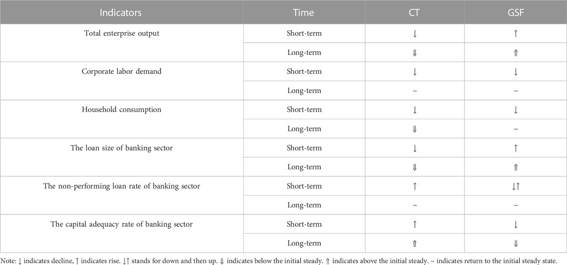
TABLE 3. The results of the long- and short-term effects of exogenous shocks on economic and financial system.

The two climate change policies have opposing effects on the economic system. The CT policy reduces total social production, while the GSF policy increases it. It can be concluded that the CT policy’s positive effect on NPEs is not enough to offset its negative effect on PEs. The implementation of an elevated CT is expected to result in an escalation of production costs for PEs, thereby leading to a subsequent enhancement in the prices of final goods produced by such firms. This phenomenon exacerbates the reduction in household consumption, which is likely to result in a corresponding decrease in output. These results are in line with previous research by Liu et al., Fischer and Springborn (2011), Meng et al. (2013), Battiston et al. (2017), Zhang and Zhang (2020), Xu and Wei (2022). Nevertheless, inconsistencies exist in the results presented by Economides and Xepapadeas (2018). It was agreed that the introduction of the CT policy would lead to a decrease in energy demand, resulting in a reduction in the use of fossil fuels. The initial reduction in fossil fuel usage hurts output, but in the long term, it has a positive effect on the economy’s productivity, resulting in higher output levels. The long-term effects of the GSF policy on PEs are found to be insignificant, while its positive impact on NPEs results in an overall increase in social output. The finding contradicts the conclusion reached by Dunz et al. (2021).

Both the CT and GSF have a short-term impact of reducing labor demand, but in the long run, they restore it to its original steady-state level. Nonetheless, the lasting impacts of these factors on household consumption exhibit dissimilarities. It is anticipated that the adoption of GSF policy will yield a decline in the aggregate need for the social labor force, thereby causing a subsequent reduction in the wage level of the household sector. This has a temporary impact on the level of consumption, but its effects are not expected to be long-lasting. The implementation of a CT policy may potentially cause a decrease in the welfare of the household sector as a result of the crowding-out effect, leading to a subsequent reduction in consumption levels.

(2) Impulse response analysis on the financial stability

The two climate change policies have opposing effects on lending rates in the financial sector. The implementation of a GSF policy reduces the interest rate for NPEs while increasing the interest rate for PEs. The overall effect on NPEs is bigger than that of the PEs. Therefore, a GSF policy results in a decline in the overall lending rate, which is detrimental to financial stability. On the contrary, a CT policy is expected to result in a rise in loan interest rates, thereby promoting financial stability.

In terms of the scale of bank loans, a GSF policy reduces the risk weight of NPEs, and causes an expansion of loan volume, which may have adverse effects on financial stability. Conversely, a CT policy is expected to reduce the loan scale, thereby promoting financial stability.

The differential effects of the two climate adaptation policies on the NPL ratio of the banking sector are observed in the short term, while their long-term impact remains consistent. The implementation of a GSF policy is expected to result in a temporary decrease followed by an increase in NPL within the banking sector. However, in the long run, the policy is anticipated to stabilize the level of NPL. The implementation of a CT policy is expected to result in a temporary rise in the NPL ratio of the banking industry, with a subsequent return to a steady state in the future, which is consistent with the findings of Bouchet and Le Guenedal (2020), Li et al. (2022). The aforementioned suggests that both policies will yield unfavorable outcomes on financial stability in the near future, as observed through the NPL ratio. However, the impact of these policies is not deemed substantial in the long run.

The impact of the two climate change policies on the CAR of the banking sector is diametrically opposed. The implementation of a GSF policy has been observed to have a negative impact on the CAR of the banking sector, thereby posing a threat to financial stability, which is similar to the findings of Thomä and Gibhardt (2019) and Dunz et al. (2021). The implementation of a CT policy is expected to result in a rise in the CAR, thereby promoting financial stability. This result is supported by Xing et al. (2024), who argued that brown capital accumulation can be discouraged through the implementation of a CT policy, which in turn contributes to financial stability.

5 Conclusion and policy implications

5.1 Conclusion

This study develops an improved dynamic stochastic general equilibrium (DSGE) model to analyze how climate change policies like carbon tax (CT) and green supporting factor (GSF) impact China’s real economy and financial stability. The model incorporates households, enterprises (polluting and non-polluting), government, and banking sector. It examines the transmission channels of the policies through credit market and risk spillovers between real economy and banking sector.

The key findings are:

• Higher intensity of both CT and GSF policies leads to greater fluctuations in financial stability indicators like interest rates, loan size, non-performing loans, and capital adequacy ratio.

• In the long run, carbon tax improves financial stability by increasing interest rates and capital adequacy ratio of banks, while reducing loan size. Green supporting factor reduces financial stability by lowering interest rates and capital adequacy ratio, and expanding loan size.

• In the short run, both carbon tax and green supporting factor have negative impact on financial stability, but the effects diminish over time.

• CT and GSF reduce corporate profits, output, and loans for polluting enterprises but increase them for non-polluting enterprises. This incentivizes the growth of non-polluting enterprises while limiting polluting enterprises.

• Implementing CT and GSF together can balance their opposing effects on economic output and financial stability. Starting with lower intensity policies reduces transition risks.

The paper makes valuable contributions by bringing together climate policies, adaptation, and financial stability; using an improved DSGE model incorporating the banking sector; and analyzing heterogeneous impacts on polluting versus non-polluting enterprises. The findings offer important implications for designing rational climate policies and facilitating green transition while maintaining financial stability.

5.2 Policy implications

The findings have significant implications for the design of climate policies and the facilitation of green transition, while also ensuring financial stability. The implementation of these policies should be carried out by financial institutions, specifically banks, and should align with the pollution levels of individual firms.

• Gradually phase in carbon taxes, starting with a low tax rate on the most emissions-intensive sectors. Slowly increase the rate and expand taxable sectors annually to ease the disturbance of climate change policies on output and finance stability.

• Implement GSF by initially reducing risk weights for NPEs’ loans. Expand eligible sectors and incrementally decrease risk weights to a small scale annually. Use GSF to support emissions-reducing technology adoption and process improvements in polluting firms. Help PEs with their green transition to lower carbon approaches.

• Employ preferential interest rates and enhanced lending facilities from policy banks and development finance institutions to provide accessible financing for green activities by NPEs.

• Create a green economic activity taxonomy to prevent misuse of preferential policies. Increase climate disclosures and stress testing.

• Coordinate fiscal, monetary, financial, and industrial policies for coherent, reinforced effects on emissions mitigation and climate risk management while supporting stability.

There are some limitations of the study. Firstly, it only examines the examination of carbon tax and green supporting factor policies due to a lack of data. Analysis might be done on additional policy options such as the introduction of carbon trading programs. Furthermore, this study employs a restricted number of economic agents and markets in its modeling approach. The inclusion of other institutions, such as equity and bond markets, has the potential to offer further valuable perspectives. It is important to acknowledge that static parameters derived from existing literature may not align perfectly with the specific characteristics of China’s economy. Enhancing the empirical estimation process has the potential to enhance the accuracy of the fit. Finally, our study exclusively concentrates on the banking sector, other financial institutions may be contemplated in subsequent research.

Data availability statement

The raw data supporting the conclusion of this article will be made available by the authors, without undue reservation.

Author contributions

Zhaosu Meng: Writing–review and editing. Xi Wang: Writing–original draft. YD: Writing–original draft.

Funding

The author(s) declare financial support was received for the research, authorship, and/or publication of this article. This research is funded by the National Social Science Foundation of China (No. 19BJY151). The National Social Science Foundation of China provided the necessary financial support for the research.

Acknowledgments

Funding from the National Social Science Foundation of China (No. 19BJY151) is gratefully acknowledged.

Conflict of interest

The authors declare that the research was conducted in the absence of any commercial or financial relationships that could be construed as a potential conflict of interest.

Publisher’s note

All claims expressed in this article are solely those of the authors and do not necessarily represent those of their affiliated organizations, or those of the publisher, the editors and the reviewers. Any product that may be evaluated in this article, or claim that may be made by its manufacturer, is not guaranteed or endorsed by the publisher.

Abbreviations

CAR, Capital adequacy ratio; CT, Carbon tax; DSGE, Dynamic stochastic general equilibrium; GSF, Green supporting factor; NPEs, Non-polluting enterprises; NPL, Non-performing loan; PEs, Polluting enterprises; SDGs, Sustainable Development Goals.

Footnotes

¹The polluting industry codes chosen for this paper are B06, B07, B08, B09, B10, B11, B12, C17, C18, C19, C22, C25, C26, C27, C28, C29, C31, C32, and D44, as per the Environmental Information Disclosure Guidance for Listed Companies published by the Ministry of Ecology and Environment in 2010 and the 2012 edition of the industry classification standards of the China Securities Regulatory Commission. The remainder are non-polluting industries.

References

Aiello, M. A., and Angelico, C. (2023). Climate change and credit risk: the effect of carbon tax on Italian banks' business loan default rates. J. Policy Model. 45 (1), 187–201. doi:10.1016/j.jpolmod.2022.11.007

CrossRef Full Text | Google Scholar

Alsamara, M., Mrabet, Z., Jarallah, S., and Barkat, K. (2019). The switching impact of financial stability and economic growth in Qatar: evidence from an oil-rich country. Q. Rev. Econ. Finance 73, 205–216. doi:10.1016/j.qref.2018.05.008

CrossRef Full Text | Google Scholar

Amiri, H., Sayadi, M., and Mamipour, S. (2021). Oil price shocks and macroeconomic outcomes; fresh evidences from a scenario-based NK-DSGE analysis for oil-exporting countries. Resour. Policy 74, 102262. doi:10.1016/j.resourpol.2021.102262

CrossRef Full Text | Google Scholar

An, Q., Zheng, L., Li, Q., and Lin, C. (2022). Impact of transition risks of climate change on Chinese financial market stability. Front. Environ. Sci. 10, 991775. doi:10.3389/fenvs.2022.991775

CrossRef Full Text | Google Scholar

Bank, W. (2017). Climate action: take urgent action to combat climate change and its impacts. https://elibrary.worldbank.org/doi/abs/10.1596/978-1-4648-1080-0_ch13 (Accessed May 12, 2023).

Google Scholar

Battiston, S., Mandel, A., Monasterolo, I., Schütze, F., and Visentin, G. (2017). A climate stress-test of the financial system. Nat. Clim. Change 7 (4), 283–288. doi:10.1038/NCLIMATE3255

CrossRef Full Text | Google Scholar

Batuo, M., Mlambo, K., and Asongu, S. (2018). Linkages between financial development, financial instability, financial liberalisation and economic growth in Africa. Res. Int. Bus. Financ. 45, 168–179. doi:10.1016/j.ribaf.2017.07.148

CrossRef Full Text | Google Scholar

Bouchet, V., and Le Guenedal, T. (2020). Credit risk sensitivity to carbon price. Available at SSRN 3574486.

Google Scholar

Bovari, E., Giraud, G., and Mc Isaac, F. (2018). Coping with collapse: a stock-flow consistent monetary macrodynamics of global warming. Ecol. Econ. 147, 383–398. doi:10.1016/j.ecolecon.2018.01.034

CrossRef Full Text | Google Scholar

Cai, D., Yan, Y., and Cheng, S. (2019). Research on the impact of carbon emission subsidies and carbon taxes on environmental quality China Population,Resources and Environment 29 (11), 59–70. doi:10.12062/cpre.20190615

CrossRef Full Text | Google Scholar

Cao, F., Zhang, Y., and Zhang, J. (2021). Carbon tax, economic uncertainty and tourism: a DSGE approach. J. Hosp. Tour. Manag. 49, 494–507. doi:10.1016/j.jhtm.2021.11.001

CrossRef Full Text | Google Scholar

Carattini, S., Heutel, G., and Melkadze, G. (2023). Climate policy, financial frictions, and transition risk. Rev. Econ. Dyn. doi:10.1016/j.red.2023.08.003

CrossRef Full Text | Google Scholar

Chu, E., and Xu, X. (2014). Government spending and economic volatility in China - based on bayesian DSGE model. Econ. Surv. 31 (02), 132–139. doi:10.15931/j.cnki.1006-1096.2014.02.019

CrossRef Full Text | Google Scholar

Cifuentes-Faura, J. (2022). European Union policies and their role in combating climate change over the years. Air Qual. Atmos. Health 15 (8), 1333–1340. doi:10.1007/s11869-022-01156-5

PubMed Abstract | CrossRef Full Text | Google Scholar

Dafermos, Y., and Nikolaidi, M. (2021). How can green differentiated capital requirements affect climate risks? A dynamic macrofinancial analysis. J. Financ. Stab. 54, 100871. doi:10.1016/j.jfs.2021.100871

CrossRef Full Text | Google Scholar

Dankert, J., van Doorn, L., Reinders, H. J., Sleijpen, O., and De Nederlandsche Bank, N. V. (2018). A green supporting factor—the right policy. SUERF Policy Note 43, 1–8. https://www.suerf.org/docx/f_99be9f83741d1275639df2c1e4d0072f_3473_suerf.pdf (Accessed September 7, 2023).

Google Scholar

Daud, S. N. M., Khalid, A., and Azman-Saini, W. (2022). FinTech and financial stability: threat or opportunity? Financ. Res. Lett. 47, 102667. doi:10.1016/j.frl.2021.102667

CrossRef Full Text | Google Scholar

Dietz, S., Bowen, A., Dixon, C., and Gradwell, P. (2016). ‘Climate value at risk’of global financial assets. Nat. Clim. Chang. 6 (7), 676–679. doi:10.1038/NCLIMATE2972

CrossRef Full Text | Google Scholar

Dombrovskis, V. (2018). Speech by vice-president dombrovskis at the high-level conference on financing sustainable growth. http://europa.eu/rapid/press-release_SPEECH-18–2421_en.html (Accessed May 7, 2023).

Google Scholar

Duan, H., Ming, X., Zhang, X., Sterner, T., and Wang, S. (2023). China’s adaptive response to climate change through air-conditioning. Iscience 26 (3), 106178. doi:10.1016/j.isci.2023.106178

PubMed Abstract | CrossRef Full Text | Google Scholar

Duan, H., Yuan, D., Cai, Z., and Wang, S. (2022). Valuing the impact of climate change on China’s economic growth. Econ. Anal. Policy 74, 155–174. doi:10.1016/j.eap.2022.01.019

CrossRef Full Text | Google Scholar

Dunz, N., Naqvi, A., and Monasterolo, I. (2021). Climate sentiments, transition risk, and financial stability in a stock-flow consistent model. J. Financ. Stab. 54, 100872. doi:10.1016/j.jfs.2021.100872

CrossRef Full Text | Google Scholar

Economides, G., and Xepapadeas, A. (2018). Monetary policy under climate change. Econ. Model. Agriculture. doi:10.2139/ssrn.3200266

CrossRef Full Text | Google Scholar

Fischer, C., and Springborn, M. (2011). Emissions targets and the real business cycle: intensity targets versus caps or taxes. J. Environ. Econ. Manag. 62 (3), 352–366. doi:10.1016/j.jeem.2011.04.005

CrossRef Full Text | Google Scholar

Gerali, A., Neri, S., Sessa, L., and Signoretti, F. M. (2010). Credit and banking in a DSGE model of the euro area. J. Money Credit. Bank. 42, 107–141. doi:10.1111/j.1538-4616.2010.00331.x

CrossRef Full Text | Google Scholar

Gu, R., Guo, J., Huang, Y., and Wu, X. (2023). Impact of the EU carbon border adjustment mechanism on economic growth and resources supply in the BASIC countries. Resour. Policy 85, 104034. doi:10.1016/j.resourpol.2023.104034

CrossRef Full Text | Google Scholar

Hong, H., Chen, Y., and Xiang, Y. (2018). A study of the effects of macroprudential management mechanisms on monetary policy. Stud. Int. Finance (09), 45–55. doi:10.16475/j.cnki.1006-1029.2018.09.005

CrossRef Full Text | Google Scholar

IPCC (2022). Climate change 2022: impacts, adaptation, and vulnerability. Contribution of working group II to the sixth assessment report of the intergovernmental panel on climate change. Cambridge University Press. https://www.ipcc.ch/report/ar6/wg2/downloads/report/IPCC_AR6_WGII_FrontMatter.pdf (Accessed September 18, 2023).

Google Scholar

Lamperti, F., Bosetti, V., Roventini, A., and Tavoni, M. (2019). The public costs of climate-induced financial instability. Nat. Clim. Change 9 (11), 829–833. doi:10.1038/s41558-019-0607-5

CrossRef Full Text | Google Scholar

Li, S., Wang, H., and Liu, X. (2022). The impact of carbon tax on financial stability. Environ. Sci. Pollut. R. 29, 55596–55608. doi:10.1007/s11356-022-19689-8

CrossRef Full Text | Google Scholar

Li, Y., Pang, D., and Cifuentes-Faura, J. (2023). Time-Varying linkages among financial development, natural resources utility, and globalization for economic recovery in China. Resour. Policy 82, 103498. doi:10.1016/j.resourpol.2023.103498

CrossRef Full Text | Google Scholar

Liu, H., Liu, Z., and Li, T. Transformational insurance and green credit incentive policies as financial mechanisms for green energy transitions and low-carbon economic development. Available at SSRN 4207694.

Google Scholar

Liu, L., and He, L. (2021). Output and welfare effect of green credit in China: evidence from an estimated DSGE model. J. Clean. Prod. 294, 126326. doi:10.1016/j.jclepro.2021.126326

CrossRef Full Text | Google Scholar

Liu, X., Cifuentes-Faura, J., Zhao, S., and Wang, L. (2023). Government environmental attention and carbon emissions governance: firm-level evidence from China. Econ. Anal. Policy 80, 121–142. doi:10.1016/j.eap.2023.07.016

CrossRef Full Text | Google Scholar

Liu, X., and Li, Z. (2022). How the structure of household asset allocation affects the efficiency of monetary policy transmission. Financial Regul. Res. (12), 60–77. doi:10.13490/j.cnki.frr.2022.12.006

CrossRef Full Text | Google Scholar

Liu, Z., Sun, H., and Tang, S. (2021). Assessing the impacts of climate change to financial stability: evidence from China. Int. J. Clim. Change Strategies Manag. 13, 375–393. doi:10.1108/IJCCSM-10-2020-0108

CrossRef Full Text | Google Scholar

Lorente, D. B., Mohammed, K. S., Cifuentes-Faura, J., and Shahzad, U. (2023). Dynamic connectedness among climate change index, green financial assets and renewable energy markets: novel evidence from sustainable development perspective. Renew. Energy 204, 94–105. doi:10.1016/j.renene.2022.12.085

CrossRef Full Text | Google Scholar

Meng, S., Siriwardana, M., and McNeill, J. (2013). The environmental and economic impact of the carbon tax in Australia. Environ. Resour. Econ. 54 (3), 313–332. doi:10.1007/s10640-012-9600-4

CrossRef Full Text | Google Scholar

Mercure, J. F., Pollitt, H., Viñuales, J. E., Edwards, N. R., Holden, P. B., Chewpreecha, U., et al. (2018). Macroeconomic impact of stranded fossil fuel assets. Nat. Clim. Chang. 8 (7), 588–593. doi:10.1038/s41558-018-0182-1

CrossRef Full Text | Google Scholar

Monasterolo, I., and Raberto, M. (2018). The EIRIN flow-of-funds behavioural model of green fiscal policies and green sovereign bonds. Ecol. Econ. 144, 228–243. doi:10.1016/j.ecolecon.2017.07.029

CrossRef Full Text | Google Scholar

Nehrebecka, N. (2021). Climate risk with particular emphasis on the relationship with credit-risk Assessment: what we learn from Poland. Energies 14 (23), 8070. doi:10.3390/en14238070

CrossRef Full Text | Google Scholar

Pelli, M. (2012). “The elasticity of substitution between clean and dirty inputs in the production of electricity,” in Paper presented at the proceedings of the conference on sustainable resource use and economic dynamics (SURED 2012) (Switzerland: Ascona).

Google Scholar

Phan, D. H. B., Iyke, B. N., Sharma, S. S., and Affandi, Y. (2021). Economic policy uncertainty and financial stability–Is there a relation? Econ. Model. 94, 1018–1029. doi:10.1016/j.econmod.2020.02.042

CrossRef Full Text | Google Scholar

Sebayang, P. (2020). The impact of the capital adequacy ratio, non-performing loan against to return on equity (case study private bank in Indonesia). SHS Web Conf 76, 01035. doi:10.1051/shsconf/20207601035

CrossRef Full Text | Google Scholar

Shang, Y., Schneider, N., Cifuentes-Faura, J., and Zhao, X. (2023). Porter in China: a quasi-experimental view of market-based environmental regulation effects on firm performance. Energy Econ. 126, 106966. doi:10.1016/j.eneco.2023.106966

CrossRef Full Text | Google Scholar

Smets, F., and Wouters, R. (2007). Shocks and frictions in US business cycles: a Bayesian DSGE approach. Am. Econ. Rev. 97 (3), 586–606. doi:10.1257/aer.97.3.586

CrossRef Full Text | Google Scholar

Sun, J. (2020). Environmental protection policy, technological innovation and dynamic effects of carbon emission intensity: simulation analysis based on three-sector DSGE model. J. Chongqing Univ. Soc. Sci. Ed. 26 (2), 31–45. doi:10.11835/j.issn.1008-5831.jg.2019.09.004

CrossRef Full Text | Google Scholar

Syed, A. A., Ahmed, F., Kamal, M. A., and Trinidad Segovia, J. E. (2021). Assessing the role of digital finance on shadow economy and financial instability: an empirical analysis of selected South Asian countries. Mathematics 9 (23), 3018. doi:10.3390/math9233018

CrossRef Full Text | Google Scholar

Tang, W., Yang, M., and Duan, H. (2023b). Temperature and corporate tax avoidance: evidence from Chinese manufacturing firms. Energy Econ. 117, 106486. doi:10.1016/j.eneco.2022.106486

CrossRef Full Text | Google Scholar

Tang, Y., Duan, H., and Yu, S. (2023a). Mitigating climate change to alleviate economic inequality under the Paris Agreement. Iscience 26 (1), 105734. doi:10.1016/j.isci.2022.105734

PubMed Abstract | CrossRef Full Text | Google Scholar

Thomä, J., and Gibhardt, K. (2019). Quantifying the potential impact of a green supporting factor or brown penalty on European banks and lending. J. Financ. Regul. Compliance 27 (3), 380–394. doi:10.1108/JFRC-03-2018-0038

CrossRef Full Text | Google Scholar

Thoma, J., and Hilke, A. (2018). The Green Supporting Factor – quantifying the impact on European banks and green finance. https://2degrees-investing.org/the-green-supporting-factor-quantifying-the-impact-on-european-banks-and-green-finance/ (Accessed May 7, 2023).

Google Scholar

Uche, E., Das, N., Bera, P., and Cifuentes-Faura, J. (2023). Understanding the imperativeness of environmental-related technological innovations in the FDI–Environmental performance nexus. Renew. Energy 206, 285–294. doi:10.1016/j.renene.2023.02.060

CrossRef Full Text | Google Scholar

Wang, B., and Song, Y. (2020). Impact of transition risk of climate change on macroeconomic and financial stability—from the perspective of stock flow consistent models. Econ. Perspect. 11, 84–99.

Google Scholar

Wang, M., Hossain, M. R., Mohammed, K. S., Cifuentes-Faura, J., and Cai, X. (2023). Heterogenous effects of circular economy, green energy and globalization on CO2 emissions: policy based analysis for sustainable development. Renew. Energy 211, 789–801. doi:10.1016/j.renene.2023.05.033

CrossRef Full Text | Google Scholar

Wang, R., Bian, Y., and Xiong, X. (2024). Analysis of the impact of rare disaster risks on small and microenterprises: based on the heterogeneous manufacturer DSGE model with financing constraints. J. Industrial Eng. Eng. Manag. 013 (01), 1–14. doi:10.13587/j.cnki.jieem.2024.01.013

CrossRef Full Text | Google Scholar

Wang, Z., and Chen, S. (2021). Research on the dynamic effects of carbon tax policy and technological impact of manufacturers under DSGE model. Science-Technology Manag. 23 (04), 57–64. doi:10.16315/j.stm.2021.04.008

CrossRef Full Text | Google Scholar

World Bank, I. F. C.MIGA. (2016). World Bank group climate change action plan 2016-2020. © World Bank, Washington, DC. http://hdl.handle.net/10986/24451 [Accessed May 20, 2023].

Google Scholar

Xing, X., Gu, X., Guo, K., and Deng, J. (2024). The interactive impact of green supporting factors on bank credit creation: an agent-based stock-flow consistent approach. North Am. J. Econ. Finance 69, 101994. doi:10.1016/j.najef.2023.101994

CrossRef Full Text | Google Scholar

Xing, X., Pan, H., and Deng, J. (2022). Carbon tax in a stock-flow consistent model: the role of commercial banks in financing low-carbon transition. Financ. Res. Lett. 50, 103186. doi:10.1016/j.frl.2022.103186

CrossRef Full Text | Google Scholar

Xu, J., and Wei, W. (2022). Would carbon tax be an effective policy tool to reduce carbon emission in China? Policies simulation analysis based on a CGE model. Appl. Econ. 54 (1), 115–134. doi:10.1080/00036846.2021.1961119

CrossRef Full Text | Google Scholar

Yan, J., and Kang, Z. (2020). Research on macro-prudential policy rules with financial stability target. Stud. Int. Finance (07), 13–24. doi:10.16475/j.cnki.1006-1029.2020.07.002

CrossRef Full Text | Google Scholar

Yang, B., Ali, M., Hashmi, S. H., and Shabir, M. (2020). Income inequality and CO2 emissions in developing countries: the moderating role of financial instability. Sustainability 12 (17), 6810. doi:10.3390/su12176810

CrossRef Full Text | Google Scholar

Yuan, Y., Li, G., and Duan, H. (2023). The achievement of multiple nationally determined contribution Goals and regional economic development in China. Resour. Energy Econ. 84 (4), 1155–1177. doi:10.1007/s10640-022-00752-4

CrossRef Full Text | Google Scholar

Zhang, J., and Zhang, Y. (2020). Examining the economic and environmental effects of emissions policies in China: a Bayesian DSGE model. J. Clean. Prod. 266, 122026. doi:10.1016/j.jclepro.2020.122026

CrossRef Full Text | Google Scholar

Zhang, T., Zhao, R., and Hou, Y. (2023). Dynamic effect on enterprise quotas in carbon emission trading mechanism. Bus. Econ. Rev. 24 (03), 105–120. doi:10.19941/j.cnki.CN31-1957/F.2023.03.008

CrossRef Full Text | Google Scholar

Zhang, W. (2009). China’s monetary policy: quantity versus price rules. J. Macroecon. 31 (3), 473–484. doi:10.1016/j.jmacro.2008.09.003

CrossRef Full Text | Google Scholar