Exploring coordinated development and its driving factors between carbon emission and ecosystem health in the southern hilly and mountainous region of China

Achieving “carbon neutrality” is an inevitable requirement for tackling global warming. As one of the national ecological barriers, the southern hilly and mountainous region (SHMR) shoulder the important mission of taking the lead in achieving “carbon peak” and “carbon neutrality”. Thus, it has important scientific significance to explore and analyze how to coordinate ecological development under the background of “double carbon action”, and it is a key step to ensure that the region achieves synergistic development of promoting economic development and improving ecosystem health. Therefore, in this study, we aimed to address these gaps by adopting a refined grid scale of 10 km × 10 km to explore the spatial-temporal distribution characteristics of carbon emissions and ecosystem health. Additionally, we established a coupling coordination model of carbon emissions intensity (CEI) and ecosystem health index (EHI) to assess the impact of natural and socio-economic factors on the coupling coordination degree (CCD) in different regions. Our findings are as follows: 1) In the SHMR region, the EHI exhibited a progressive development trend, with spatially increasing values from the south to the north. 2) The spatial discrepancy in CEI has been on the rise, which assumed an increase of 4.69 times, and with an increasingly pronounced pattern of spatial imbalance. Carbon emissions tend to concentrate more in the eastern and northern areas, while they are comparatively lower in the western and southern regions. 3) The R² of geographical weighted regression model (GWR) is all above 0.8, and the CCD between CEI and EHI demonstrated a positive developmental state. However, most regions still displayed an imbalanced development, albeit with a slight increase in areas exhibiting a more balanced development state. 4) The driving forces of natural and socio-economic factors had a dual-factor and non-linear enhancement effect on the CCD. The influence of natural factors on CCD has gradually diminished, whereas the influence of socio-economic factors has progressively strengthened.

1 Introduction

In the context of the 2030 Agenda for Sustainable Development, the achievement of the Sustainable Development Goals (SDGs) necessitates a comprehensive consideration of the social, economic, and environmental dimensions (UNFCCC, 2015; ICSU, 2017). Sustainable Development Goal number 11 aims to promote the establishment of inclusive, secure, resilient, and sustainable cities and human settlements. This implies the need for harmonized progress in both economic development and ecological environmental protection. Consequently, how to mitigate the significant impact of rapid urbanization on the ecological environment and achieve a green and sustainable path of development is a pivotal concern demanding attention from all nations during the process of urbanization (Ayre and Landis, 2012; Bayliss et al., 2012; Awuah et al., 2020). China, with its rapid urbanization and industrialization, has emerged as the largest global emitter of carbon. The rapid economic growth has notably influenced carbon emissions from ecosystems due to frequent land use changes. Consequently, alterations in land use patterns exert significant effects on ecosystems, which subsequently impact the services they provide. It is important to note that land use changes not only affect the spatial distribution, extent, and intensity of carbon emissions but also modify ecosystem health by altering the spatial distribution of biodiversity, regional resources, and ecosystem types. Thus, achieving a balance between socio-economic development and ecosystem health has become a universal and critical challenge, particularly for China (Lin and Christina, 2019). The Southern Hilly and Mountainous Region (SHMR) represents a crucial component of China’s ecological security, playing a fundamental role in regulating local and even global climate, facilitating vegetation restoration, and conserving soil and water resources (Tian et al., 2022). However, due to the concentration of population, land resources in this region have been excessively exploited over an extended period. The long-standing irrational utilization of land resources has resulted in both a low regional production level and a deterioration of the ecological environment. Hence, investigating the spatiotemporal interplay between carbon emissions and ecosystem health in the SHMR holds immense significance for achieving green and sustainable development within this region. Furthermore, it has far-reaching implications for guiding the healthy and sustainable green development of the national ecosystem as a whole.

Both domestic and international research has extensively scrutinized the decoupling effects of carbon emissions and economic growth across various scales, including national levels (Liu et al., 2023), provincial (Zhang et al., 2019), urban (Mcgeeid and York, 2019) and regional (Khan et al., 2020) carbon emissions (Munir et al., 2020), an explanation of the mechanism of carbon emissions from a single land class (Chen et al., 2019b), influencing factors (Xie et al., 2020; Jia et al., 2023), change rules (Yu et al., 2018), efficiency (Zhang et al., 2022), and the relationship between land class change and carbon source/sink (Zhang et al., 2013). A large number of studies have been conducted from the perspectives of spatial differences and associations of carbon emissions (Zhao et al., 2022).

As a crucial focus of macroecology research, the concept of ecosystem health possesses distinct characteristics pertaining to spatial and temporal scales. Among the various scales considered for the study of macro ecosystem management, the region emerges as the most appropriate spatial scale for investigating and evaluating ecosystem health. Regional ecosystem health refers to the capacity of each regional ecosystem to consistently and sustainably provide ecosystem service functions within a specific spatial and temporal framework, while maintaining its own health (Yan et al., 2016). Regional ecosystem health assessment has increasingly gained importance as a research direction within the field of ecosystem health assessment. It amalgamates the evaluation of type quality, quantitative structure, and spatial pattern, with a central focus on ecosystem service functions. Several studies have already been conducted on ecosystem health assessment, encompassing different spatial-temporal and regional scales (Chen et al., 2018), such as provinces (Peng et al., 2017), urban agglomerations (Peng et al., 2018), rivers (Zheng et al., 2008; Xia et al., 2019), and wetlands (Wu and Ding, 2019). The evaluation index system for ecosystem health comprises a set of interconnected and mutually constrained indicators, necessitating the selection of indicators that are both relevant and independent. These indicators should comprehensively reflect the level of health and its changing trends in the ecosystem, while accurately reflecting the objectives of ecosystem management and evaluation. Two main models have been employed in constructing the index system: the pressure-state-response (PSR) model (Shear et al., 2003) and the vigor-organization-resilience (VOR) model (Borja et al., 2006). Additionally, the vigor-organization-resilience-ecosystem service (VORS) model has been developed to address the limitations of the previous two models, as they only measure the state of the ecosystem and external disturbances, disregarding the ability to evaluate the provisioning of ecosystem services (Shen et al., 2016; Chen et al., 2019a). Consequently, this study establishes a comprehensive index framework for evaluating ecosystem health in the SHMR region based on the VORS model.

Few studies have explored the spatial relationship between carbon emissions and ecosystem health. Coupling coordination means that two or more systems interact with each other or within the system and affect and restrict each other, and finally reach a benign interaction of coordinated development relationship, the basic premise of which is that there is a certain connection between the factors coupled with each other (Tian et al., 2022). In other words, carbon emission and ecosystem health form a closely related complex coupled system in the competition and cooperation of mutual support and mutual restriction. By regulating subsystems that have a great influence on the overall evolution of the coupled system, all subsystems are promoted to tolerate each other in the unity of oppositions and eventually tend to coordinate development. Thus, this study constructed a coupling coordination model based on carbon emission and ecosystem health to explore the coupling effect and coordination development level between carbon emission intensity (CEI) and ecosystem health index (EHI) on a spatiotemporal scale. What’s more, the heterogeneity or non-stationarity of spatial data relationship is one of the research hotspots in the field of spatial statistics and related applications, and the development of local spatial statistical analysis technology is the key link. Geographically weighted regression (GWR) analysis method was used to solve the geographically weighted regression analysis model, so as to quantitatively reflect the heterogeneity or non-stationary characteristics of spatial data relations by estimating parameters that vary with different spatial locations. Thus, this study further introduced GWR model to explore the spatial heterogeneity of EHI and CEE. In addition, with SHMR ecosystem health as the core, this study aims to propose a new method that can directly verify the specific extent of carbon emission’s negative effects on SHMR ecosystem. What’s more, the influencing factors of EHI and CEI coupling systems are also discussed. Traditional methods such as the regression model (Chi et al., 2018b), correlation analysis (Bae et al., 2010) and principal component analysis (Cheng et al., 2018) are usually used for this. However, due to the intricate nature of geographical processes, it is not feasible to quantify the interaction and interplay between influencing factors that contribute to spatial differentiation of CCD using traditional statistical regression analysis methods (Ye et al., 2012). In contrast, the geographical detector model offers a unique analytical approach that not only assesses the individual contribution of each factor to the coupled system but also examines the interactive influence of multiple factors on the coupled system (Wang et al., 2016). This interactive analysis aspect is notably absent in other existing studies. Thus, building upon these considerations, this study employed the geodetector model to quantitatively analyze the influencing factors of the CEI and EHI coupling system.

Within the mentioned context, this study primarily investigates the following issues concerning carbon emission and ecosystem health in the SHMR region: 1) What are the spatial-temporal patterns of heterogeneity exhibited by the CEI and EHI within the SHMR region? 2) How does the EHI respond to changes in the CEI during the study period in the SHMR? 3) How does the state of coupling and coordination between the CEI and EHI vary across different regions within the SHMR during the study period? 4) What are the primary drivers that influence the development of coupling systems between the CEI and EHI during the study period? Are there any regional disparities observed in this regard?

1.1 Study area

In Figure 1, the topography of the SHMR exhibits an undulating terrain, complemented by a well-developed water system, numerous rivers, and abundant water resources. This region boasts a wealth of biological species and a diverse array of soil types. The SHMR harbors a flourishing ecosystem, comprising forests, wetlands, grasslands, and more. These ecosystems are characterized by their remarkable biodiversity and impressive carbon storage capacity, rendering them of paramount importance in the context of land use carbon emissions. The SHMR encompasses a diverse range of land use types, including farmland, woodland, and urban areas. It stands out as a vital ecological sanctuary in China, necessitating urgent measures for ecosystem preservation and the attainment of sustainable development. Over the past two decades, the SHMR has encountered significant transformations in land use patterns and ecological landscapes due to intensified human intervention. As a consequence, ecosystems have experienced a precipitous decline, leading to the deterioration of their critical functions pertaining to ecosystem services. These changes bear profound implications for the overall wellbeing of the ecosystems. Concurrently, the surge in carbon emissions has engendered environmental predicaments that pose a substantial threat to social productivity and introduce considerable risks to the natural ecosystem within the SHMR region. The stark contrast between ecological health and economic development has garnered widespread attention. Therefore, enhancing the ecosystem health of the SHMR and achieving carbon peaking and carbon neutrality assume paramount significance in pursuit of green and sustainable development.

FIGURE 1

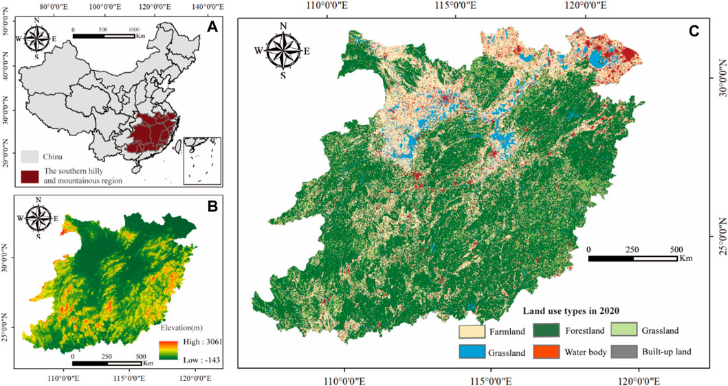
FIGURE 1. (A) Map of study area; (B) The DEM of the area; (C) The Land use and land cover in 2020.

It is noteworthy that, in comparison to certain urban conglomerations, the SHMR exhibits a more intricate interplay of topographic and geomorphic features, thereby endowing its ecosystem with complexity and diversity. Moreover, the SHMR’s warm and humid climate, abundant vegetation, and diverse land use types distinguish it from grasslands and plateaus, which tend to possess relatively homogenous ecosystems. Consequently, the SHMR exerts a more pronounced influence on land use carbon emissions. In summary, the SHMR presents an ideal milieu for investigating the correlation between ecosystem health and carbon emissions.

1.2 Data sources and processing

The spatial datasets employed in this investigation were primarily sourced from the esteemed Resources and Environmental Science Data Centre and National Academy of Sciences of China, accessible at the URL http://www.resdc.cn. These datasets encompassed a comprehensive land use classification framework, delineated into six distinct categories, namely cultivated land, forest land, grassland, water bodies, construction land, and unused land. The resolution of these datasets was finely delineated at 1 km × 1 km, ensuring a meticulous and granular analysis. Furthermore, the study also integrated climate data of equally impressive resolution (1 km × 1 km), encapsulating average annual precipitation and average annual temperature. Additionally, datasets pertaining to net primary productivity (NPP), digital elevation model (DEM), population density (PD), and gross domestic product density (GDPD) were also included, all meticulously resolved at the spatial resolution of 1 km × 1 km. To augment the comprehensive analysis, various statistical metrics were culled from the esteemed Statistical Yearbook of the SHMR provinces, spanning the time frame from 1990 to 2020. These encompassed vital aspects such as food production, energy consumption, and other pertinent variables, thereby enriching the comprehensiveness and robustness of the investigation.

1.3 Methods

1.3.1 Quantifying carbon emission efficiency (CEI)

The calculation of carbon emission is to multiply the area of each land use type with its corresponding carbon emission coefficient, and then carry out the sum calculation. The calculation formula is below (Zhang et al., 2014):

${\mathit{E}}_{\mathit{K}}=\sum {\mathit{e}}_{\mathit{i}}=\sum {\mathit{S}}_{\mathit{i}}\times {\mathit{\delta }}_{\mathit{i}}(1)$

In this equation, the variable $E_K$ represents the direct carbon emissions, while $e_i$ signifies the carbon emissions associated with each land use type. Moreover, $S_i$ and ${\delta }_i$ represent the area and carbon emission coefficient of land use type $i$, respectively, indicating the carbon emission coefficient specific to each land-use type. To establish the carbon emission coefficients for each land use type, relevant literature and the specific conditions of the study area were meticulously examined. The carbon emission coefficients were determined as follows: cultivated land (0.422), forest land (−0.644), grassland (−0.022), water bodies (−0.253), and unused land (−0.005) (Cai et al., 2005). The carbon emissions attributed to build-up land were calculated based on fossil energy consumption and subsequently divided by the area to derive the carbon emission intensity of such land. The estimation of carbon emissions from build-up land was accomplished through an indirect estimation method, wherein data from the China Energy Statistical Yearbook were integrated along with various energy consumption patterns and corresponding carbon emission coefficients (Table 1) (Lai et al., 2016).

TABLE 1

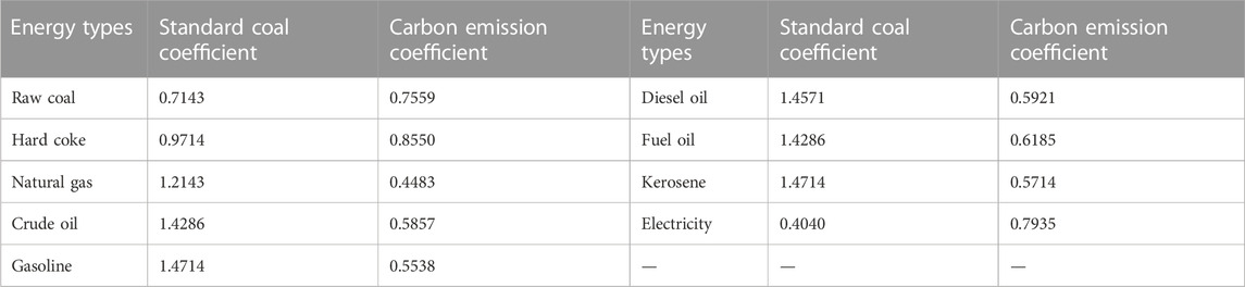
TABLE 1. Standard coal coefficient and carbon emission coefficient of different energy source.

Carbon emission calculation formula of build-up land (Wu et al., 2022):

${\mathit{E}}_{\mathit{\eta }}=\sum {\mathit{e}}_{\mathit{i}}=\sum {\mathit{E}}_{\mathit{i}}\times {\mathit{\mu }}_{\mathit{i}}\times {\mathit{\epsilon }}_{\mathit{i}}(2)$

In this equation, the variable $E_{\eta }$ represents the carbon emission emanating from built-up land, whereas $e_i$ signifies the carbon emission generated by the consumption of energy $i$. Furthermore, $E_i$ denotes the consumption of energy $i$, while ${\mu }_i$ represents the conversion coefficient of energy $i$ consumption into standard coal. Additionally, the carbon emission coefficient of energy $i$ is signified by ${\epsilon }_i$.

The CEI of land use is established by considering both the area and carbon emission coefficient associated with each land use type within a grid. Consequently, a higher carbon emission intensity implies a greater carbon emission within the cell (Friedlingstein et al., 2010).

${\mathit{C}}_{\mathit{l}\mathit{u}\mathit{c}\mathit{c}}={\displaystyle \sum _{\mathit{i}=\mathbf{1}}^{\mathit{n}}}\frac{{\mathit{S}}_{\mathit{i}}{\mathit{P}}_{\mathit{i}}}{\mathit{S}}(3)$

In this equation, denoted by $C_{lucc}$, the CEI is calculated. The variables $S_i$ and $P_i$ correspond to the area and carbon emission coefficient, respectively, of land use type $i$ within the grid. Additionally, the total area of the grid is represented by the variable $S$. The CEI of build-up land is the value of carbon emissions of build-up land within each grid.

1.3.2 Constructing the ecosystem health assessment framework

An ecologically robust regional ecosystem should uphold its integrity, exhibit inherent self-regulatory capabilities, and offer consistent and sustainable ecosystem services to humanity. Drawing upon a comprehensive review of existing research findings, the vigor-organization-resilience-services (VORS) model has been chosen as the foundation for developing the EHI evaluation framework within the context of the SHMR. The EHI is expressed as (He et al., 2019):

$\mathit{E}\mathit{H}\mathit{I}=\sqrt[\mathbf{4}]{\mathit{V}*\mathit{O}*\mathit{R}*\mathit{S}}(4)$

Wherein, EHI denotes the ecosystem health index, while V, O, R, and S represent ecosystem vigor, ecosystem organization, ecosystem resilience, and ecosystem service, respectively. Employing the range standardization method, the EHI, V, O, R, and S were standardized on a scale of 0–1 (Mingde et al., 2010).

${\mathit{A}}_{\mathit{i}}=\frac{{\mathit{X}}_{\mathit{i}}-\mathit{min}\left({\mathit{X}}_{\mathit{i}}\right)}{\mathit{max}\left({\mathit{X}}_{\mathit{i}}\right)-\mathit{min}\left({\mathit{X}}_{\mathit{i}}^{\prime }\right)}(5)$

In this equation, $A_i$ represents the dimensionless value of the $ith$ indicator, and $\max \left(X_i\right)$ signifies the maximum value of the $ith$ indicator.

1) Ecosystem vigor is a vital ecosystem function, representing a key manifestation of system metabolism or primary productivity. The Normalized Vegetation Index (NDVI) serves as a valuable indicator of vegetation’s productive capacity. Moreover, the strong correlation between NDVI and Net Primary Productivity (NPP) means that NPP serves as an ideal metric for characterizing ecosystem vigor in the present study.

2) Ecosystem organization is the interaction between various components of a system, reflecting the stability and complexity of the system structure. The more complex the structure, the healthier the ecosystem. Furthermore, this index layer is subject to the influence of landscape heterogeneity, the configuration of the landscape, and the degree of landscape connectivity. The utilization of the Shannon Diversity Index (SHDI) and Shannon Evenness Index (SHEI) was employed to effectively capture and elucidate the intricate patterns of spatial heterogeneity. That is, the higher the spatial heterogeneity, the more stable the landscape structure, the stronger the landscape organization ability. To encapsulate the landscape connectivity, the Interspersion and Juxtaposition Index (IJI), Division Index (DIVISION), and Contagion Index (CONTAG) were employed as insightful metrics. The higher the landscape connectivity, the more favorable the inter-species migration and the communication between different patches, the stronger the landscape organization. The index of perimeter-area fractal dimension (PAFRAC) was used to express the landscape shape. Thus, the formula is as follows (Chi et al., 2018a):

$\mathit{O}=\mathbf{0.4}*\mathit{L}\mathit{H}+\mathbf{0.4}*\mathit{L}\mathit{C}+\mathbf{0.2}*\mathit{I}\mathit{C}=\left(\mathbf{0.2}*{\mathit{L}\mathit{C}}_{\mathbf{1}}+\mathbf{0.2}*{\mathit{L}\mathit{C}}_{\mathbf{2}}\right)+\left(\mathbf{0.1}*{\mathit{L}\mathit{C}}_{\mathbf{3}}+\mathbf{0.15}*{\mathit{L}\mathit{C}}_{\mathbf{4}}+\mathbf{0.15}*{\mathit{L}\mathit{C}}_{\mathbf{5}}\right)+\mathbf{0.2}*\mathit{P}\mathit{A}\mathit{F}\mathit{R}\mathit{A}(6)$

Where $LH$ alludes to the intricate landscape heterogeneity, $LC$ signifies the profound landscape connectivity, and $IC$ pertains to the captivating landscape shape. Additionally, ${LC}_1$ and ${LC}_2$ correspond to the succinct acronyms “SHDI” and “SHEI” respectively, while ${LC}_3$, ${LC}_4$, and ${LC}_5$ elegantly represent the metrics of Interspersion and Juxtaposition Index (IJI), Division Index (DIVISION), and Contagion Index (CONTAG) in that order.

3) Ecosystem resilience epitomizes the inherent ability of an ecological system to uphold its structural equilibrium in the face of perturbations caused by human activities. Past investigations have established that land utilization can serve as a reliable gauge of ecosystem resilience. To quantify this resilience, we assign Resilience Coefficients based on the distinct land use categories. The comprehensive measure of ecosystem resilience is then computed through the weighted aggregation of both the spatial extent and ecological resilience coefficients associated with diverse land use classifications within the given region, as delineated below (Kang et al., 2018):

$\mathit{R}={\displaystyle \sum _{\mathit{i}=\mathbf{1}}^{\mathit{n}}}\frac{{\mathit{A}}_{\mathit{i}}}{{\mathit{A}}_{\mathit{I}}}\times {\mathit{R}\mathit{C}}_{\mathit{i}}(7)$

In this equation, $R$ symbolizes the resilience of the urban ecosystem within the district under examination. $A_I$ corresponds to the total land area encompassed by the study region, whereas $A_i$ represents the specific area occupied by the respective land use types. Furthermore, ${RC}_i$ denotes the ecological restoration coefficient associated with the $ith$ land use classification. Drawing upon prior research findings, the ecological resilience coefficients for cultivated land, forest land, grassland, water bodies, built-up land, and unused land are documented as 0.3, 0.8, 0.7, 0.8, 0.2, and 1, respectively.

4) Ecosystem services encompass an array of invaluable products and advantages bestowed upon human society by the natural ecological environment. These services are quantified through the measure of ecosystem service power, which highlights the monetized value attributed to said services. In this study, the revised calculation of ecosystem services per unit area was undertaken by integrating the land use types specific to the SHMR region, utilizing Xie Gaodi’s refined scale of ecological services in Chinese ecosystems. Incorporating the ESV per unit area scale proposed and updated in 2017, the economic value corresponding to grain production per unit area of farmland was adopted as the benchmark ESV, representing a standard equivalent factor of 1.

$\mathit{E}\mathit{S}\mathit{V}={\displaystyle \sum _{\mathit{i}=\mathbf{1}}^{\mathit{n}}}{\mathit{A}}_{\mathit{i}}\times {\mathit{V}\mathit{C}}_{\mathit{i}}(8)$

In the equation, $ESV$ represents the total value of ecosystem services analyzed in this study, $A_i$ denotes the area (in hectares) of the ith type of land use, and ${VC}_i$ represents the ecosystem service value coefficient for the ith type of land use.

1.3.3 Geographically weighted regression model

Based on the fact that random distribution of variables in the classical OLS model does not have independent spatial characteristics, also required a high degree of mutual independence between regions. Thus, the classical model is modified by introducing spatial differences and spatial correlations. That is, geographical weighted regression (GWR) introduced the spatial attributes of data, and explores the heterogeneity of spatial data through the estimation of different spatial relations of geographic space and regional parameters with spatial dependency (Chris et al., 1996). In the pursuit of investigating the spatial heterogeneity of the CEI on the EHI from a global standpoint, this study employed a GWR model. The formulation utilized in this analysis can be expressed as follows (Sciences et al., 2017):

${\mathit{Y}}_{\mathit{i}}={\mathit{\beta }}_{\mathbf{0}}\left({\mathit{\mu }}_{\mathit{i}},{\mathit{v}}_{\mathit{i}}\right)+{\displaystyle \sum _{\mathit{k}}}{\mathit{\beta }}_{\mathit{k}}\left({\mathit{\mu }}_{\mathit{i},}{\mathit{v}}_{\mathit{i}}\right){\mathit{X}}_{\mathit{i}\mathit{k}}+{\mathit{\epsilon }}_{\mathit{i}}(9)$

In this equation, we denote $Y_i$ as the dependent variable, representing the observed values of interest. The explanatory variable, $X_{ik}$, signifies the covariates considered in the analysis. The position function, $\left({\mu }_i,v_i\right)$, captures the spatial coordinates of each observation i. The constant term of regression, ${\beta }_0$, represents the intercept, while ${\beta }_k$ denotes the vector of parameters to be estimated. Lastly, ${\epsilon }_i$ represents the random error term accounting for unobserved factors.

1.3.4 Coupling coordination analysis of carbon emission and ecosystem health

“Coupling” is a physical concept that means the phenomenon in which two (or more) systems or forms of motion affect each other through various interactions. The phenomenon of “coupling” exists in all fields of society and has universal significance. In economics, coupling refers to the phenomenon that two or more economic subsystems influence each other and even cooperate through various interactions. The concept of coupling degree pertains to the extent of interaction and interconnectivity within a system or its constituent elements. Specifically, coupling coordination degree (CCD) serves as an indicator of the level of interaction and interdependence among subsystems, underpinned by the underlying coupling degree. Therefore, the CCD model of CEI and EHI coupling development is constructed based on the following formulas (He et al., 2017):

$\mathit{C}={\left\{\frac{\mathit{U}\left(\mathit{\alpha }\right)\times \mathit{U}\left(\mathit{\beta }\right)}{{\left[\frac{\mathit{U}\left(\mathit{\alpha }\right)+\mathit{U}\left(\mathit{\beta }\right)}{\mathbf{2}}\right]}^{\mathbf{2}}}\right\}}^{\frac{\mathbf{1}}{\mathbf{2}}}(10)$

$\mathit{T}=\mathit{a}\mathit{U}\left(\mathit{\alpha }\right)+\mathit{b}\mathit{U}\left(\mathit{\beta }\right)(11)$

$\mathit{C}\mathit{C}\mathit{D}=\sqrt{\mathit{C}\times \mathit{T}}(12)$

In the given equation, the variable $D$ represents the value of CCD, where $U\left(\alpha \right)$ denotes the value of EHI and $U\left(\beta \right)$ signifies the value of CEI. The variable $C$ signifies the coupling degree of the aforementioned subsystems, while $T$ represents the comprehensive level of coordination between these subsystems. Lastly, the variables a and b refer to the respective contributions made by the two subsystems.

The study recognizes the paramount significance of both economic development and ecological protection. Hence, the CEI and EHI subsystems were accorded equal importance, with the values of a and b being set at 0.5 each.

To enhance the evaluation of the coupling development state between CEI and EHI in SHMR, the classification criteria and types of CCD were established, drawing upon earlier research works (Table 2) (Cui et al., 2019).

TABLE 2

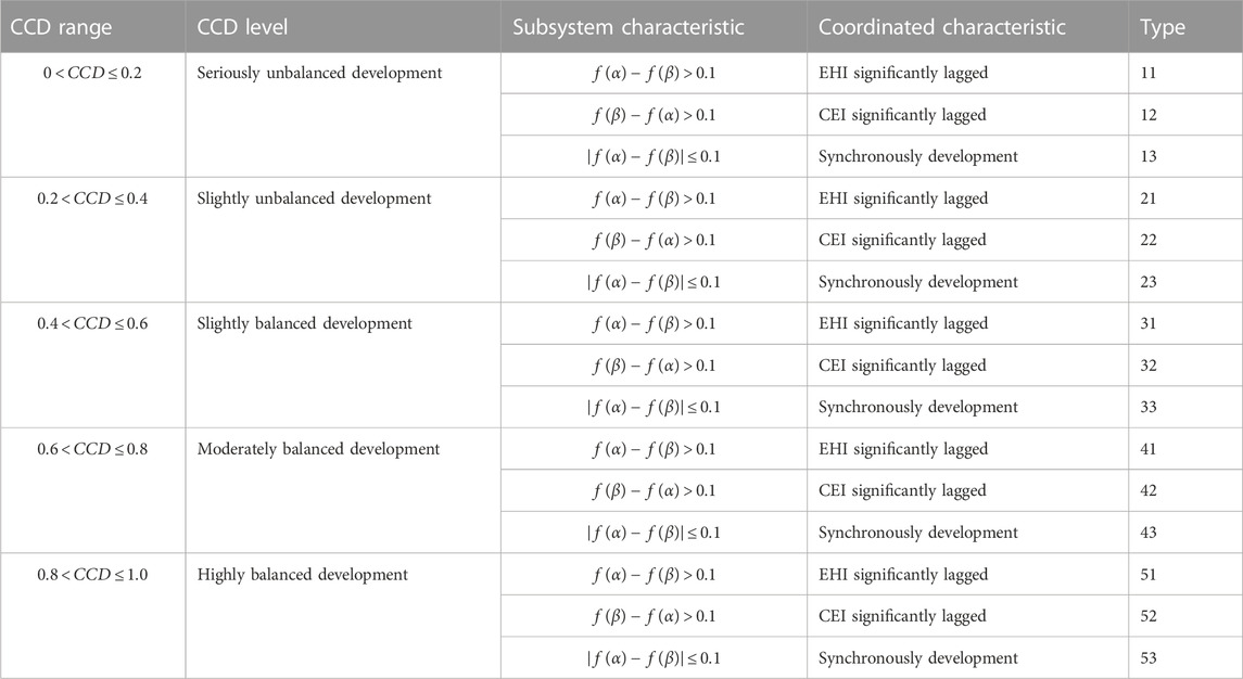
TABLE 2. The coupling coordination types and characteristic of CEI and EHI.

1.3.5 Geographical detector model (GDM)

As a statistical method used to reveal the driving factors of spatial differentiation, geographic detector is an important new method to detect the spatial pattern and causes of geographical elements, and has been gradually applied to the research in various fields such as urban development. This study mainly adopted factor detection and interaction detection to measure the effect intensity of driving factors on CCD in SHMR. The formula is as follows (Wang et al., 2020):

$\mathit{q}=\mathbf{1}-\frac{{\sum }_{\mathit{h}=\mathbf{1}}^{\mathit{L}}{\mathit{N}}_{\mathit{h}}{\mathit{\sigma }}_{\mathit{h}}^{\mathbf{2}}}{{\mathit{N}}_{\mathit{\sigma }}^{\mathbf{2}}}(13)$

In the given equation, the $q$ value, ranging from 0 to 1, serves to unveil the degree of contribution of independent variable factors to dependent variable factors, thereby enabling the identification of the dominant factor of CCD in this study. A higher $q$ value suggests a greater influence of the independent variable on the dependent variable. $L$ represents the layer of independent variable. $N_h$ and N denote the number of unit grids of layer h and the entire region, respectively. ${\sigma }_h^2$ and ${\sigma }^2$ represent the variance of CCD in layer $h$ and the entire region, respectively.

The level of economic development exerts a substantial impact on regional land use carbon emissions, necessitating a heightened focus on ecological preservation during urban land expansion. The intricate operation mechanism of ecosystems is influenced by a multitude of natural and socio-economic factors, thereby shaping ecosystem health. Consequently, this study aims to elucidate the influencing factors within the coupling coordination system of carbon emissions and ecosystem health, as illustrated in Table 3. Natural influencing factors were characterized through the selection of climate, topographic factors, geology, and resource endowments. Climatic conditions were specified by indicators such as annual average temperature, annual average humidity, and annual average precipitation. Topographic conditions were represented by elevation and relief degree of the land surface. Resource endowment was assessed through the selection of indicators such as net primary productivity (NPP), forest coverage, and biological abundance index. Human activities and the level of economic development primarily characterized socio-economic factors. To be more precise, the level of human activity was gauged through the human disturbances index, GDP density, and population density.

TABLE 3

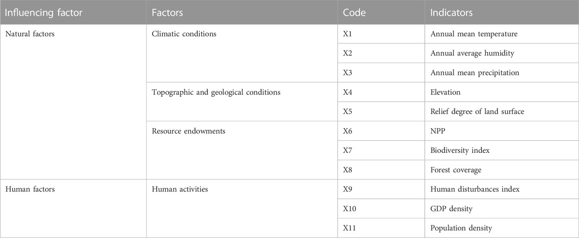
TABLE 3. Index system of influencing factors.

The computation methodology for determining the relief degree of the land surface in this study draws upon established and pertinent research in the field. The formula is below (Qiao et al., 2018):

$\mathit{R}\mathit{D}\mathit{L}\mathit{S}=\left\{\left[\mathit{Max}\left(\mathit{H}\right)-\mathit{Min}\left(\mathit{H}\right)\right]\times \left[\mathbf{1}-\mathit{P}\left(\mathit{A}\right)/\mathit{A}\right]\right\}/\mathbf{500}(14)$

In the above equation, the relief degree of the land surface (RDLS) is computed using the following parameters: $\mathit{Max}\left(H\right)$ and $\mathit{Min}\left(H\right)$ represent the uppermost and lowermost elevations within the region, respectively. $P\left(A\right)$ denotes the extent of flat land area in square kilometers (km²), while $A$ encompasses the overall area of the research unit, measuring 64 km². For the purpose of this investigation, we have classified any land area with a slope equal to or less than 2° as flat terrain.

The computation methodology for the biodiversity index in this investigation aligns with established and pertinent scholarly inquiries. The formula is below (Fitter, 2012):

$\mathbf{\text{BI}}={\mathbf{A}}_{\text{bio}}\times \left(\mathbf{0.11}\times {\mathbf{A}}_{\mathbf{1}}+\mathbf{0.35}\times {\mathbf{A}}_{\mathbf{2}}+\mathbf{0.21}\times {\mathbf{A}}_{\mathbf{3}}+\mathbf{0.28}\times {\mathbf{A}}_{\mathbf{4}}+\mathbf{0.04}\times {\mathbf{A}}_{\mathbf{5}}+\mathbf{0.01}\times {\mathbf{A}}_{\mathbf{6}}\right)/{\mathbf{A}}_{\text{total}}(15)$

${\mathbf{A}}_{\text{bio}}=\mathbf{100}/\mathbf{\text{MA}}\mathbf{X}=\mathbf{100}/\mathbf{0.35}=\mathbf{285.71}(16)$

Here, the biodiversity index (BI) is determined by the normalized coefficient ($A_{bio}$) derived from the areas of cultivated land, forestland, grassland, water body, build-up land, and unused land ($A_1-A_6$), all within the confines of the research unit. The total area of the research unit is denoted as $A_{total}$.

The calculation model of human disturbances index is established based on a large amount of data of human disturbances and land use, thereby the quantitative description of human disturbance in a certain area was realized. To reflect the spatial characteristics of human disturbances, the human disturbances values were divided into 5 levels by Jenks natural breaks method. The human disturbances index formula is as follows (Chen et al., 2010):

$\mathit{H}\mathit{D}=\frac{{\sum }_{\mathit{i}=\mathbf{1}}^{\mathit{m}}{\mathit{W}}_{\mathit{i}}\times {\mathit{S}}_{\mathit{i}}}{\mathit{S}}(17)$

Here, the human disturbances value (HD) for each grid is determined by the human disturbances index ($W_i$) associated with each land use type ($i$), as established in prior research. The area of each land use type ($i$) is denoted as $S_i$, while the total area of the grid is represented by $S$.

2 Results

2.1 Dynamic changes of carbon emission intensity

The CEI in SHMR exhibited a consistent upward trajectory from 1990 to 2020, as depicted in Figure 2. Throughout the duration of the study, the CEI demonstrated a remarkable degree of stability, with minimal drastic fluctuations. From 1990 to 2020, CEI in the northern region of SHMR showed a gradual upward trend. For each region, the CEI decreases from north to south. The overall economic strength of the northern region is increasing at the same time, the CEI is also increasing. The low value of CEI is mostly distributed in the south, showing an overall increase. The maximum carbon emission intensity increases from 3.61 t/hm² in 1990 to 101.42 t/hm² in 2020, an increase of 4.69 times. The number of grids falling in the Ⅰ region decreased year by year, especially from 2000 to 2005 decreased by 78.3%, and there was a shift to the Ⅱ region. The grids in the second zone increased first and then decreased, and the southern region, where the land use type is mainly cultivated land, has been stable in this zone since 2010. The growth rate of grid number in the Ⅲ region is the highest, accounting for 46.36% of the total grid number in 2020, which is mostly consistent with the distribution range of cultivated land. The grids in the Sections 4, 5 increased year by year and were in clumps, mainly concentrated in the construction land with active human activities.

FIGURE 2

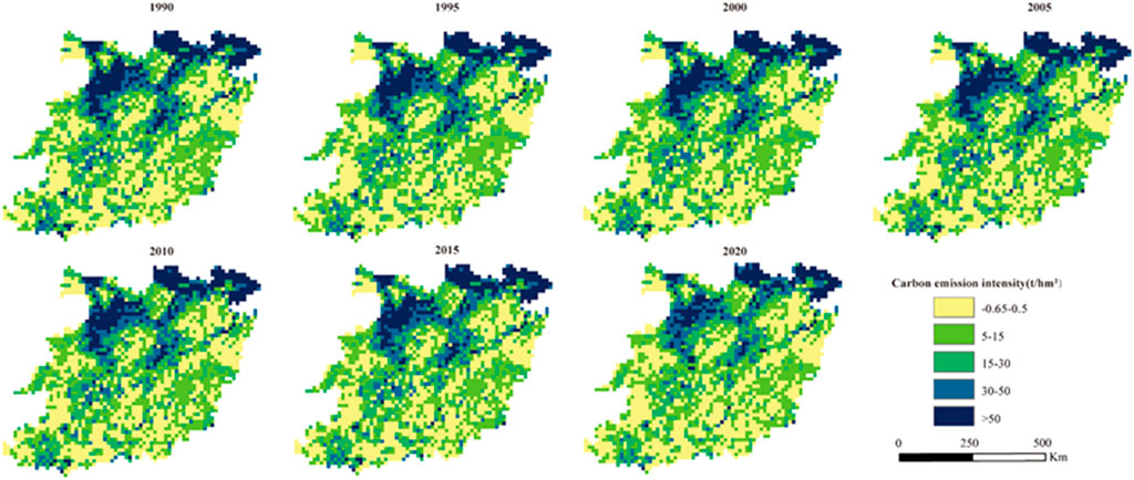
FIGURE 2. The spatial-temporal distribution of carbon emission intensity (CEI) in SHMR, 1990–2020.

2.2 Dynamics of ecosystem health

Figure 3 depicted the spatial-temporal distribution of indicators that represent the health of ecosystems in SHMR. These indicators encompass ecosystem vigor (EV), ecosystem organization (EO), ecosystem resilience (ER), and ecosystem services (ES). Notably, the regions exhibiting the most pronounced changes in EV were predominantly situated in the northwestern part of SHMR, displaying a gradual decline in magnitude from north to south. In terms of temporal progression, EV demonstrated an upward trend from 1990 to 2005, followed by a gradual decline from 2005 to 2020. Regarding EO, the regions with notable variations were primarily concentrated in the northwestern part of SHMR, although discernible changes were also evident in the southern region. Over the course of the study period, SHMR as a whole exhibited an increasing trend in EO from 1990 to 2020. However, from 2000 to 2020, the southeastern region experienced a declining trend in EO. In terms of spatial scale, both ER and ES exhibited a comparable distribution pattern. The values of ER and ES were notably higher in regions characterized by abundant forest coverage, whereas regions encompassing vast areas of construction land and unused land demonstrated lower levels of ER and ES. Considering the temporal dimension, ER and ES displayed a gradual decline throughout the SHMR from 1990 to 2020. However, a noteworthy decrease in ER and ES was observed from 2005 to 2020, particularly in the northern and northeastern regions of SHMR.

FIGURE 3

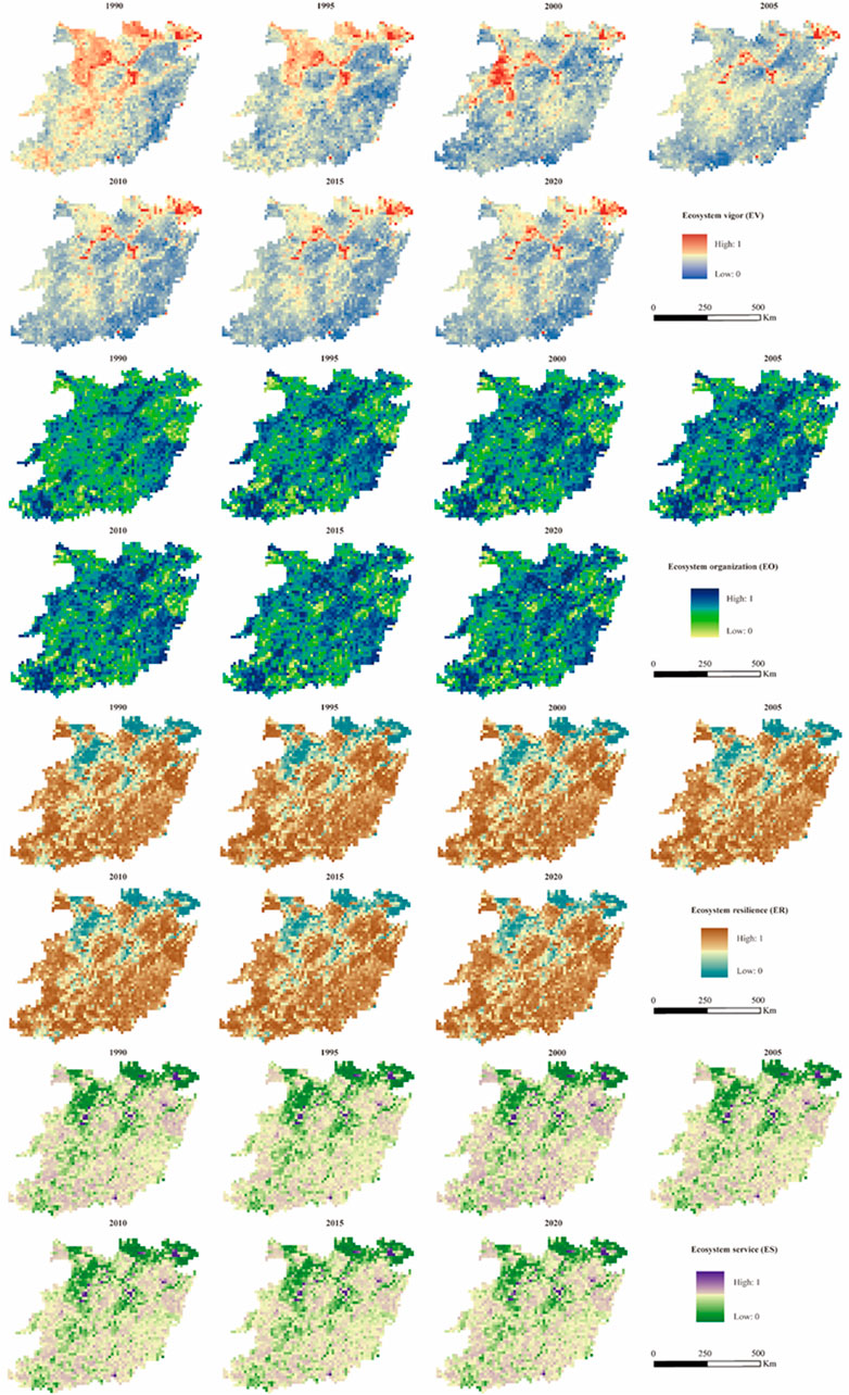
FIGURE 3. The ecosystem health index (EHI) at grid scale, 1990–2020. EV is ecosystem vigor, EO is ecosystem organization, ER is ecosystem resilience, and ES is ecosystem service.

The spatiotemporal distribution of EHI in the SHMR region was shown in Figure 4. Specifically, in spatial scale, EHI showed a trend of increasing gradually from north to south. The distribution area of high EHI value areas showed an increasing trend, mainly distributed in the southern region with high forest coverage and wide water distribution. The distribution area of high EHI value area showed a decreasing trend, mainly distributed in the northern build-up land and unused land distribution area. In terms of time scale, the overall EHI of SHMR showed a significant increase trend from 1990 to 2005, but showed a gradually decreasing trend after 2005 to 2020.

FIGURE 4

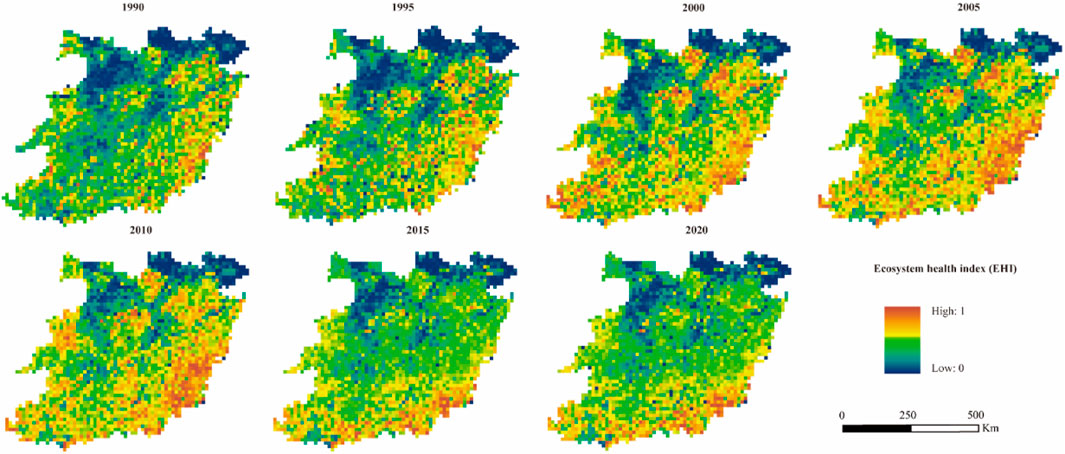
FIGURE 4. The ecosystem health index (EHI) in SHMR, 1990–2020.

2.3 Spatial correlation analysis between carbon emission and ecosystem health

In this study, geographical weighted regression model (GWR) was selected to analyze the spatial impacts of carbon emissions on ecosystem health in SHMR (Figure 5), which with the consideration of spatial spillover effects between the above subsystem. Table 4 listed the parameters in the GWR model, we found that R² is all above 0.8, which indicated that GWR model has a good fitting effect, and EHI and CEI both showed obvious clustering phenomenon.

FIGURE 5

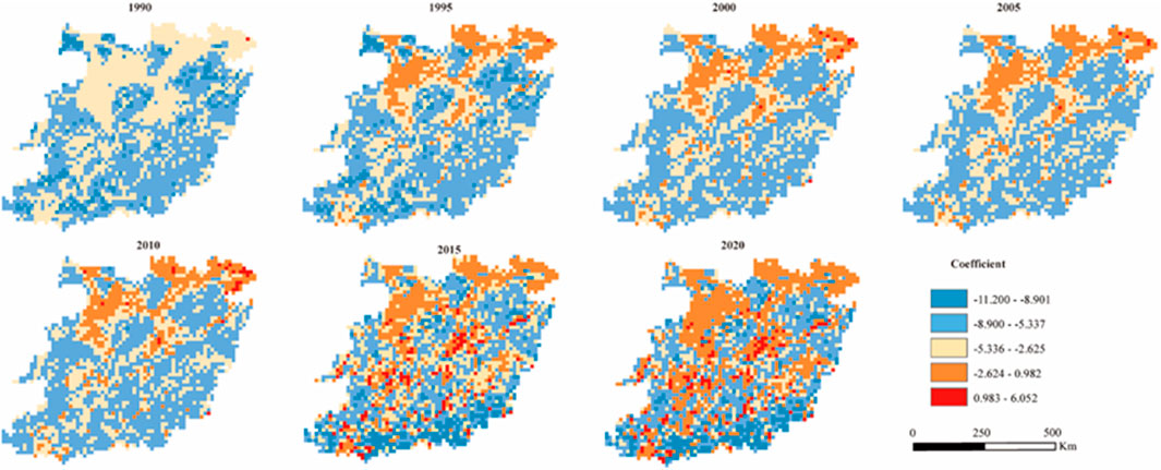
FIGURE 5. Spatial distribution of regression coefficients for the carbon emission intensity (CEI) and ecosystem health index (EHI), 1990–2020.

TABLE 4

TABLE 4. Estimation parameters for GWR models, 1990–2020.

What’s more, in SHMR from 1990 to 2005, the regression coefficients of CEI and EHI were negative on the whole, and the negative effect between CEI and EHI was dominant. This revealed that with the increase of CEI value, there was a large negative impact in SHMR regional ecosystem. In other words, with the acceleration of regional urbanization, a higher CEI value has been generated, which has a more significant interference with EHI value and a more prominent damage to ecosystem health. It is worth noting that the regression coefficient began to show a positive value from 2010, indicating that the spatial spillover effect of CEI on EHI began to show a positive effect. Moreover, the positive distribution area of the regression coefficient showed an increasing trend from 2010 to 2020, and it was mainly distributed in the areas with more distribution of forest land and water body. Although these regions have higher CEI value, the spatial spillover effect of CEI on EHI began to show a positive effect. But at the same time, forest land and water body can provide higher EHI value, so CEI and EHI will have a positive relationship.

2.4 Quantification of the coupling coordination degree between carbon emission and ecosystem health

2.4.1 Temporal changes of coupling coordination degree levels

Against the backdrop of rapid globalization, the relentless expansion of urban land and the accelerated surge in carbon emissions have exerted immense pressure on the local ecological milieu. Consequently, for the realization of regional green and sustainable development, it becomes imperative to attain a harmonious and symbiotic relationship between carbon emissions and ecological health while striving for high-caliber economic progress. To this end, the CCD model is employed to quantitatively analyze the coupling and coordination levels and patterns of CEI and EHI across spatial and temporal dimensions (Figure 6). Specifically, a higher CCD value signifies a more robust coupling degree between the two subsystems of carbon emission and ecosystem health, thereby facilitating the emergence of a novel, organized structure. Conversely, a lower CCD value indicates a less desirable state of coordination. In this regard, within the context of advanced carbon emission development, it becomes crucial to curtail the level of EHI to the utmost extent. Thus, the “EHI significantly lagged” CCD type represents the optimal state of coordination. Significantly, as outlined in Table 2, it is imperative for the CCD value to exceed 0.4 to achieve a somewhat balanced equilibrium between ecosystem services and carbon emissions.

FIGURE 6

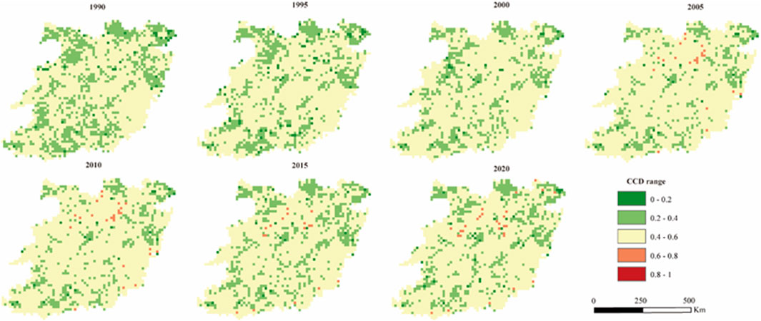
FIGURE 6. The Spatial-temporal characteristic of coupling coordination degree (CCD), 1990–2020.

2.4.2 Spatial distribution of coupling coordination degree types

Figure 7 showed the CCD values and types from 1990 to 2020 in SHMR. As can be seen from Figure 7, CCD types in SHMR present obvious differences in spatial-temporal distribution. From 1990 to 1995, the main types of CCD were “21” and “22”, that is, the CEI and EHI of SHMR showed a slightly unbalanced development state. Specifically, during 1990–1995, CEI lagged behind in most southern regions of SHMR, while EHI lagged behind in most northern regions. This is consistent with the spatial-temporal distribution of CEI and EHI described above, in the northern region of SHMR, the level of economic development in the northern region is more advanced, whereas the southern region lags behind in comparison. Moreover, from 1990 to 1995, there were more “32” type of CCD, and the distribution area of “22” type showed a decreasing trend, which indicates that CEI and EHI showed a slightly balanced development state in the development process of SHMR. In 2000, the distribution of CCD types changed significantly, the distribution area of “21” and “22” types were greatly reduced, and a new CCD distribution type “31” appeared, that is, in the state of CEI and EHI slightly balanced development, EHI showed a lagging development state. Moreover, from 2000 to 2020, the distribution area of “31” type showed an obvious trend of increase, indicating that during this period, SHMR paid more attention to economic development, and the development of EHI was significantly affected, showing a significant lag state. We must ardently foster the advancement of ecological civilization, enhance the quality and resilience of the ecosystem, and propel the SHMR regions towards a trajectory of green and sustainable development.

FIGURE 7

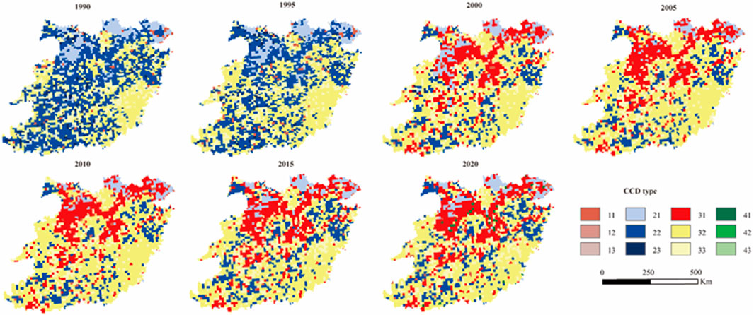
FIGURE 7. Spatial distribution pattern of the coupling coordination degree (CCD) type, 1990–2020 (Seriously unbalanced development: “11”, “12”, “13”; Slightly unbalanced development: “21”, “22”, “23”; Slightly balanced development: “31”, “32”, “33”; Moderately balanced development: “41”, “42”, “43”).

2.5 Driving factors of regional differences in coupling coordination degree

2.5.1 Single factor detector analysis of coupling coordination degree

The q value, as gauged by the geographic detector, serves as a metric for quantifying the impact of each influencing factor. Notably, a higher q value corresponds to a greater degree of influence exerted by the factor on the spatial differentiation of CCD, as elucidated in Table 5. Furthermore, statistical analysis reveals significant disparities among the factors, affirming the relative soundness of the factors chosen for this study. Moreover, discernible discrepancies emerge in terms of the influence various factors wield on the spatial differentiation of CCD between 1990 and 2020.

TABLE 5

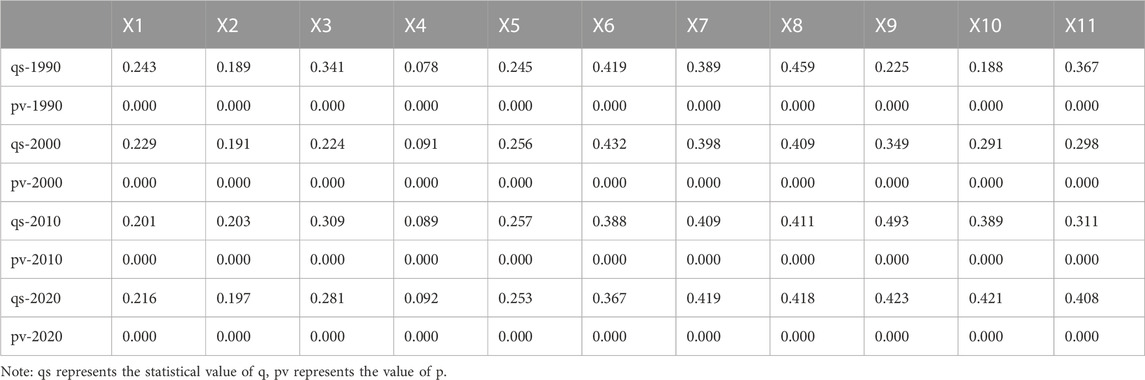
TABLE 5. q statistic and p values of detection factors, 1990–2020.

As depicted in Table 5, it is evident that the q value associated with forest coverage consistently ranks highest between 1990 and 2010, underscoring its pivotal role in determining the spatial distribution of CCD (Table 3). In fact, its explanatory power with respect to the spatial pattern of CCD escalated to 61.8% by 2020. Notably, the q value linked to the human disturbances index (X9) underwent substantial changes during the period spanning from 1990 to 2020, surging from 0.225 to 0.423. This signifies a bolstering influence of the human disturbances index in elucidating the spatiotemporal characteristics of CCD, surpassing even the significance of forest coverage. Additionally, the q values associated with GDP density (X10) and population density (X11) exhibited an upward trajectory, with explanatory powers of 55.34% and 10.05% respectively, by 2020. Conversely, the q values pertaining to annual average humidity and elevation remained consistently low, signaling their limited capacity to explicate the temporal and spatial dynamics of CCD, and thus their marginal role in the observed changes.

2.5.2 Interaction detector analysis of coupling coordination degree

The interaction detector allowed for the identification of interactions between distinct influencing factors, X, and evaluated whether their combined presence amplifies or diminishes the explanatory capacity of the dependent variable, Y. It also determined if the influence of these factors on Y was independent of each other. The detection results were obtained through a comparison of the individual q values and the interaction q values [q (X1∩X2)]. These results can be broadly categorized into three types: weakening, mutual enhancement, and nonlinear enhancement (Figure 8).

FIGURE 8

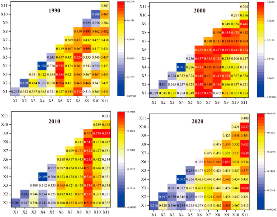
FIGURE 8. Interaction detection of factors, 1990–2020.

The Figure 8 vividly depicted the enhanced interaction between the two distinct influencing factors. This enhancement was primarily characterized by the augmentation of the two factors, as well as a nonlinear amplification. Notably, no weakening or independent relationship was observed. Specifically, the period spanning 1990–2020 has witnessed a diminishing effect of most natural factors on CCD, while the influence of socio-economic factors has steadily intensified. For example, annual mean precipitation (X3) decreases from 0.341 to 0.280, and NPP (X6) decreases from 0.419 to 0.367, and the influence on CCD shows a weakening trend. Human disturbances index (X9) increased from 0.225 to 0.423, and GDP density (X10) increased from 0.188 to 0.421, gradually becoming a high impact factor promoting the coordinated development of CEI and EHI system coupling. It is worth mentioning that forest coverage (X8) has maintained a relatively significant effect from 1990 to 2020, which may be related to the high forest coverage in SHMR. Further, in 2020, the absolute value of interaction between NPP (X6) and human disturbances index X9 reaches 0.653, higher than the single interaction of X6 and X9; The absolute value of the interaction between NPP (X6) and GDP density (X10) is 0.531, which is higher than the single interaction of X6 and X10. The absolute value of the interaction between annual mean temperature (X1) and population density (X11) reached 0.413, which was higher than the single interaction value of X1 and X11. This indicated that with the rapid economic development, the influence and limitation of natural conditions such as precipitation and humidity on CCD in the SHMR region were gradually weakened.

3 Discussion

3.1 Staged response of ecosystem health to carbon emission

The precise delineation of the spatial-temporal progression of ecosystem health, along with a comprehensive comprehension of its dynamic association with the carbon emission process, lies at the crux of achieving a harmonious and sustainable nexus between regional environmental preservation and the enhancement of ecosystem wellbeing (Ran et al., 2021; Song et al., 2015). Moreover, in order to assess the extent of the influence of carbon emission on ecosystem health within the study area, as well as the potential spatial spillover effects, the spatial-temporal response characteristics of carbon emission to ecosystem health in the SHMR region were ascertained through the utilization of the GWR model (Table 6).

TABLE 6

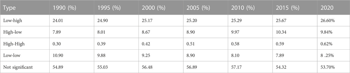
TABLE 6. Percentages of different types of LISA clusters, 1990–2020.

The urban agglomerations are undergoing a rapid and transformative phase of social and economic development, where frequent land use changes exert a direct influence on carbon emission dynamics. Alterations in land use patterns, spatial arrangements, and management strategies not only impact the ecosystem, but also disrupt the delicate equilibrium of the carbon cycle system, thereby affecting the CEI. During the initial stage of carbon emission, specifically from 1990 to 2005, the CEI did not exhibit a substantial impact on the EHI. Throughout this period, the spatial distribution proportions of the “Low-high” and “High-low” types experienced marginal shifts, increasing from 24.10% to 25.20% and from 7.89% to 8.90%, respectively. This gradual progression suggests that higher CEI values gradually demonstrate a more pronounced interference on EHI values. From 2005 to 2015, the influence of CEI on EHI became notably significant. The proportion of the “Low-high” spatial distribution rose from 25.20% to 25.67%, while the proportion of the “High-low” spatial distribution increased from 8.90% to 10.34%. Concurrently, swift and efficient carbon emission reduction efforts resulted in an 11.34% decline in the proportion of the “Low-low” spatial distribution, while the proportion of the “High-high” spatial distribution witnessed a 15.69% increase. This pattern emerges due to the rapid urbanization in the SHMR region, wherein population siphoning leads to a substantial influx of rural residents into urban areas, causing congestion. Vigorous human activities act as drivers for accelerated carbon emission, while the expansion of construction land and heightened energy consumption result in significant encroachments upon forested and cultivated lands. Consequently, carbon emissions from construction land experience a noteworthy surge. Previous studies have already indicated that continuous population growth plays a pivotal role in propelling carbon emission dynamics, with the expanding proportion of construction land holding significance in this process (Liu et al., 2023). However, in reality, the vast expansion of urban land fails to align harmoniously with the demands of urban production and living, and the growth rate of the population evidently lags behind the expansion of regional urban land. This contradiction is not exclusive to China alone but is a common phenomenon in the developmental trajectory of global cities (Zhao et al., 2022). In 2020, our country proactively pursued the goal of “Carbon peaking and carbon neutrality,” implementing a series of measures across various domains of life, production, and ecology. Consequently, the nation’s economic development has transitioned towards a stage of high-quality growth, signifying a transitional phase in carbon emission dynamics. During this period, the influence of CEI on EHI has diminished within the SHMR region. The proportion of the “Low-high” spatial distribution has reached its pinnacle at 26.60%, marking the highest value throughout the study period, while the proportion of the “High-low” spatial distribution stands at 9.84%. This finding further underscores the fact that SHMR’s urbanization process is transitioning towards a high-quality, green, and sustainable phase, thereby mitigating the impact of rapid carbon emission on the ecosystem’s green and sustainable development. In essence, during the pursuit of high-quality economic development, greater attention should be directed towards the expansion of urban construction land and the enhancement of the development mode. Macro-level land use control should be strengthened, and a concerted effort should be made to promote the efficient, collaborative, and sustainable development of carbon emission and ecosystem services within the SHMR region.

3.2 The influence mechanism of control variables on coupling coordinated degree

The findings of this study revealed significant regional variations in the driving forces of CCD within the SHMR. At the regional level, during the year 1990, the pivotal factors influencing the coupling system between carbon emission and ecosystem health were identified as forest coverage, net primary productivity (NPP), and biodiversity index. This can be attributed, in part, to the inherent natural endowment of the SHMR itself, with forested land covering a remarkable 70% of the total area. The region also displays conspicuous spatial heterogeneity in its ecosystems (Ren et al., 2018). Furthermore, ecological management initiatives in the SHMR, such as reforestation efforts, land consolidation, and afforestation programs, have contributed to the expansion of forested areas, thereby augmenting the proportion of broadleaf and coniferous forests (Sohil and Sharma, 2020). Furthermore, it is worth noting that the topography of the SHMR exhibits noticeable fluctuations, with vegetation coverage surpassing 60% in the region. This abundant vegetation plays a pivotal role in climate regulation. Several studies have indicated that climatic factors serve as the primary determinants of regional ecological sensitivity (Yao et al., 2012). Through the intricate interplay between precipitation patterns and land use intensity, these factors influence the growth and distribution of vegetation within the region. However, it is crucial to acknowledge that with the rapid economic development and continuous urbanization in the SHMR, socio-economic factors, such as GDP and the human disturbance index, will emerge as the principal drivers influencing the coupling system of carbon emission and ecosystem health in the year 2020. Particularly in the central and eastern regions of the SHMR, population density has increased significantly, accompanied by dense population distribution and a robust GDP. Unfortunately, this dense population distribution and rapid economic progression have given rise to a series of issues, including environmental pollution and ecosystem degradation, resulting in a high CEI value and a low EHI value. Consequently, these regions exhibit a lagging state of development in terms of EHI.

Remarkably, the development of CCD in the SHMR is significantly influenced by both natural and socioeconomic factors, and their interaction yields intriguing outcomes. Previous research has established that alterations in wetland, grassland, and forest ecosystems are intricately shaped by a combination of intricate climatic forces and human activities (Wang et al., 2022). In the year 2020, the distribution area of CCD types in the SHMR region displayed a moderately balanced pattern, with the “31” type experiencing a substantial upward trajectory. This further underscores the prevailing state of lagging development in terms of EHI. Concurrently, the q-values for natural factors, such as forest coverage (X8), annual mean precipitation (X3), and the relief degree of the land surface (X5), were all 0.45. Similarly, the socioeconomic factors of human disturbances index (X9) and GDP density (X10) yielded q-values of −0.34. Notably, the absolute value of the interaction between forest coverage (X8) and human disturbances index (X9) was found to be 0.23. Likewise, the absolute value of the interaction between annual mean precipitation (X3) and GDP density (X10) reached 0.45 The continuous expansion of urbanized areas has led to the encroachment upon vast stretches of farmland and forested land within the region, resulting in the direct attenuation of regional biodiversity and the fragmentation of ecosystem structures. The q-value for the biodiversity index (X7) has exhibited a decline from 0.12 in 1990 to 0.34 in 2020. Consequently, it is imperative to prioritize the preservation of the natural advantages inherent to the SHMR, consistently upholding the region’s high vegetation coverage. Moreover, meticulous attention must be directed towards addressing extreme climatic events. Concurrently, the administrative authorities must proactively recalibrate the regional economic industries and guide the judicious distribution of the population to mitigate the adverse consequences of human interference.

3.3 Implications for ecosystem management and sustainable development

Determining the regional differences of the coupling coordination degree of carbon emission and ecosystem service subsystems in SHMR region and their driving factors will not only provide important guidance and suggestions for the development of differentiated ecosystem protection and ecosystem health improvement in SHMR region. In addition, it can scientifically reduce carbon emission and improve ecosystem health under the background of ensuring the current high-quality economic development. It is usually in the high CEI value regions, which have low EHI values and are mostly in a slightly coupling coordinated development state with lagging ecosystem health.

Owing to the siphon effect, a substantial concentration of high-caliber workforce and advanced production technology converges within this particular region, enabling effective management of the input-output relationship during the process of urban land expansion. This allows for seizing policy opportunities to drive the transformation and upgrading of the industrial structure, optimizing the allocation of land inputs, and ultimately achieving the green and sustainable development of various urban sectors. Simultaneously, the pace of urban land expansion can be judiciously regulated to prevent the destruction of the ecosystem’s landscape organization resulting from imprudent reclamation of cultivated land. This ensures a harmonious development trajectory, striking a balance between high-quality economic growth and ecological environmental preservation. Moreover, the implementation of ecological protection and restoration initiatives, such as land reforestation, assumes great significance as it improves vegetation coverage and mitigates ecological and environmental predicaments like soil erosion, thereby enhancing the overall health of the ecosystem. These projects are particularly crucial in regions boasting high EHI values and relatively lower CEI values. Consequently, it is imperative to curtail the influence of natural factors on the coupling system of carbon emission and ecosystem services. This necessitates comprehensive consideration of the natural endowment conditions within the SHMR region, empowering the strengthening of protective functions such as meteorological disaster monitoring and fostering the implementation of ecological protection and restoration initiatives. Furthermore, urban development within these regions should exhibit reduced reliance on construction land investments, thereby significantly bolstering the efficiency of regional resource integration and utilization.

3.4 Future work

The examination of ecosystem contributions and their potential ramifications on carbon emissions has been the subject of numerous investigations, employing both empirical measurement and simulation analyses. Notably, these studies have shed light on the commendable carbon storage capacity of forest ecosystems, while also identifying wetlands and marine ecosystems as capable carbon sinks. Concomitantly, addressing the issue of land use carbon emissions has also been a focal point of research endeavors, with a particular emphasis on devising strategies to curtail such emissions and safeguard the integrity of ecosystems. Prominent measures include the enhancement of agricultural practices, the adoption of sustainable urban planning and construction models, and the promotion of ecological restoration and conservation efforts. These studies serve as a foundational bedrock for the formulation of policies geared towards carbon reduction and sustainable development. Thus, the nature of land use holds considerable sway over ecosystem robustness and carbon emissions. Subsequent investigations could delve into unraveling the repercussions of diverse land use types on ecosystem functions and services, as well as assessing the corresponding levels of carbon emissions. Moreover, agriculture, as a pivotal terrestrial endeavor, bears substantial influence on ecosystem welfare and carbon emissions. Prospective research endeavors could be steered towards ground-breaking agricultural technological innovations, aiming to curtail agricultural carbon emissions through the implementation of scientific farming methods and the optimization of agricultural production chains. Furthermore, a comprehensive analysis could be conducted on the intricate carbon cycle processes within agro-ecosystems, seeking ways to enhance the carbon storage capacity of farmland by improving soil quality, judicious crop selection, and rational fertilization practices. Lastly, urbanization, an indisputable force in land use dynamics, bears profound ramifications for both ecosystem health and carbon emissions. Future research undertakings could concentrate on fostering ecological restoration and protection amidst the urbanization process, while also endeavoring to diminish carbon emissions in urban planning and construction. This would concomitantly enhance the stability and perpetuation of urban ecosystems. Additionally, novel strategies pertaining to urban greening, urban agriculture, and urban water resources management can be explored as viable approaches to ameliorate urban carbon emissions and bolster ecosystem wellbeing.

5 Conclusion

In this study, carbon emission and ecosystem health evaluation index systems were established respectively, and dynamically evaluated the carbon emission intensity (CEI) and ecosystem health level (EHI) in SHMR. Utilizing the Global Geographically Weighted Regression (GWR) model, this study extended our understanding of the spatial ramifications of carbon emissions on ecosystem health within the SHMR region. Furthermore, a comprehensive coupling system encompassing CEI and the EHI has been devised, enabling a quantitative assessment of the development level and nature of this coupling system. This approach allowed for a more nuanced examination of the intricate interplay between carbon emissions and ecosystem health in the SHMR area. Ultimately, the geodetector model was employed to quantitatively analyze the spatially differentiated influencing factors impacting the coupling system between ecosystem health and carbon emissions. The resulting insights can be summarized as follows:

(1) Within the SHMR region, spanning the period from 1990 to 2020, the EHI has shown a discernible northward spatial increase, accompanied by marked global spatial autocorrelation and localized spatial agglomeration. Concurrently, the CEI has exhibited an escalating level of spatial differentiation, manifesting a conspicuous spatial imbalance. The distribution pattern of carbon emissions can be described as “predominantly eastern and lesser in the western regions, and more pronounced in the northern areas while relatively diminished in the southern regions.”

(2) Over the period spanning from 1990 to 2020, the coupling coordination degree (CCD) between the CEI and the EHI within the SHMR region has exhibited a gradual, yet promising, increase. However, upon scrutinizing the spatial distribution of the coupling coordination type pertaining to carbon emission and ecosystem health, an unbalanced development still dominates most of the SHMR, with slightly unbalanced development being the prevalent type. Nevertheless, the area manifesting slightly balanced development is observed to be on the rise. Notably, the CEI and EHI in the northwest and southwest regions of the SHMR are relatively high, with the majority exhibiting CEI lag and a coupling coordinated development type of CEI and EHI synchronous lag.

(3) Our single factor analysis revealed that the human disturbance index, forest coverage, GDP density, and biodiversity index were vital factors contributing to the spatial differentiation of the carbon emission and ecosystem health coupling system in the SHMR region. The factor interaction test further demonstrated that natural and socio-economic factors were not mutually exclusive and, in fact, exhibited a dual-factor and non-linear enhancement effect on the CCD. Over time, as the social and economic landscape has evolved, the influence of natural factors on CCD has weakened, while the influence of social and economic factors has gradually intensified. In other words, our findings suggest that in ecologically vulnerable regions like the SHMR, socio-economic factors play an increasingly catalytic role in augmenting the impact of natural factors.

Data availability statement

The raw data supporting the conclusions of this article will be made available by the authors, without undue reservation.

Author contributions

HQ: Conceptualization, Data curation, Formal Analysis, Investigation, Methodology, Project administration, Resources, Software, Supervision, Validation, Visualization, Writing–original draft, Writing–review and editing. CY: Data curation, Writing–review and editing. WW: Data curation, Writing–review and editing. LG: Conceptualization, Funding acquisition, Writing–review and editing.

Funding

The author(s) declare financial support was received for the research, authorship, and/or publication of this article. This work was supported by the National Key Research and Development Program of China (2022YFF1303001).

Acknowledgments

We would like to thank the National Key Research and Development Program of China.

Conflict of interest

The authors declare that the research was conducted in the absence of any commercial or financial relationships that could be construed as a potential conflict of interest.

Publisher’s note

All claims expressed in this article are solely those of the authors and do not necessarily represent those of their affiliated organizations, or those of the publisher, the editors and the reviewers. Any product that may be evaluated in this article, or claim that may be made by its manufacturer, is not guaranteed or endorsed by the publisher.

References

Awuah, K. F., Jegede, O., Hale, B. A., and Siciliano, S. D. (2020). Introducing the adverse ecosystem service pathway as a tool in ecological risk assessment. Environ. Sci. Technol. 54, 8144–8157. doi:10.1021/acs.est.9b06851

PubMed Abstract | CrossRef Full Text | Google Scholar

Ayre, K. K., and Landis, W. G. (2012). A bayesian approach to landscape ecological risk assessment applied to the upper grande ronde watershed, Oregon. Hum. Ecol. Risk Assess. 18, 946–970. doi:10.1080/10807039.2012.707925

CrossRef Full Text | Google Scholar

Bae, D. Y., Kumar, H. K., Han, J. H., Kim, J. Y., Kim, K. W., Kwon, Y. H., et al. (2010). Integrative ecological health assessments of an acid mine stream and in situ pilot tests for wastewater treatments. Ecol. Eng. 36, 653–663. doi:10.1016/j.ecoleng.2009.11.027

CrossRef Full Text | Google Scholar

Bayliss, P., Dam, R. A. V., and Bartolo, R. E. (2012). Quantitative ecological risk assessment of the magela creek floodplain in kakadu national park, Australia: comparing point source risks from the ranger uranium mine to diffuse landscape-scale risks. Hum. Ecol. Risk Assess. 18, 115–151. doi:10.1080/10807039.2012.632290

CrossRef Full Text | Google Scholar

Borja, Á., Galparsoro, I., Solaun, O., Muxika, I., Tello, E. M., Uriarte, A., et al. (2006). The European Water Framework Directive and the DPSIR, a methodological approach to assess the risk of failing to achieve good ecological status. Estuar. Coast. Shelf Sci. 66, 84–96. doi:10.1016/j.ecss.2005.07.021

CrossRef Full Text | Google Scholar

Cai, Z., Kang, G., Tsuruta, H., and Mosier, A. (2005). Estimate of CH4 emissions from year-round flooded rice fields during rice growing season in China. Pedosphere 15, 66–71.

Google Scholar

Chen, A., Zhu, B.-Q., Chen, L.-D., Wu, Y.-H., and Sun, R.-H. (2010). Dynamic changes of landscape pattern and eco-disturbance degree in Shuangtai estuary wetland of Liaoning Province, China. Chin. J. Appl. Ecol. 21, 1120–1128.

PubMed Abstract | Google Scholar

Chen, C., Wang, Y., and Jia, J. (2018). Public perceptions of ecosystem services and preferences for design scenarios of the flooded bank along the Three Gorges Reservoir: implications for sustainable management of novel ecosystems. Urban For. Urban Green. 34, 196–204. doi:10.1016/j.ufug.2018.06.009

CrossRef Full Text | Google Scholar

Chen, C., Wang, Y., Jia, J., Mao, L., and Meurk, C. D. (2019a). Ecosystem services mapping in practice: a Pasteur’s quadrant perspective. Ecosyst. Serv. 40, 101042. doi:10.1016/j.ecoser.2019.101042

CrossRef Full Text | Google Scholar

Chen, D., Lu, X., Liu, X., and Wang, X. (2019b). Measurement of the eco-environmental effects of urban sprawl: theoretical mechanism and spatiotemporal differentiation. Ecol. Indic. 105, 6–15. doi:10.1016/j.ecolind.2019.05.059

CrossRef Full Text | Google Scholar

Cheng, X., Chen, L., Sun, R., and Kong, P. (2018). Land use changes and socio-economic development strongly deteriorate river ecosystem health in one of the largest basins in China. Sci. Total Environ. 616-617, 376–385. doi:10.1016/j.scitotenv.2017.10.316

PubMed Abstract | CrossRef Full Text | Google Scholar

Chi, Y., Shi, H., Zheng, W., Sun, J., and Fu, Z. (2018a). Spatiotemporal characteristics and ecological effects of the human interference index of the Yellow River Delta in the last 30years. Ecol. Indic. 39, 1219–1220.

Google Scholar

Chi, Y., Zheng, W., Shi, H., Sun, J., and Fu, Z. (2018b). Spatial heterogeneity of estuarine wetland ecosystem health influenced by complex natural and anthropogenic factors. Sci. Total Environ. 634, 1445–1462. doi:10.1016/j.scitotenv.2018.04.085

PubMed Abstract | CrossRef Full Text | Google Scholar

Chris, H., Brunsdon, A., Stewart, F., Martin, E., and Charlton, L. (1996). Geographically weighted regression: a method for exploring spatial nonstationarity. Geogr. Anal. 28, 281–298. doi:10.1111/j.1538-4632.1996.tb00936.x

CrossRef Full Text | Google Scholar

Cui, D., Chen, X., Xue, Y., Li, R., and Zeng, W. (2019). An integrated approach to investigate the relationship of coupling coordination between social economy and water environment on urban scale - a case study of Kunming. J. Environ. Manage. 234, 189–199. doi:10.1016/j.jenvman.2018.12.091

PubMed Abstract | CrossRef Full Text | Google Scholar

Fitter, N. A. H., Norris, K., and Fitter, A. H. (2012). Biodiversity and ecosystem services: a multilayered relationship. Trends Ecol. Evol. 27, 19–26. doi:10.1016/j.tree.2011.08.006

PubMed Abstract | CrossRef Full Text | Google Scholar

Friedlingstein, P., Houghton, R. A., Marland, G., Hackler, J., Boden, T. A., Conway, T. J., et al. (2010). Update on CO2 emissions. Nat. Geosci. 3, 811–812. doi:10.1038/ngeo1022

CrossRef Full Text | Google Scholar

He, J., Pan, Z., Liu, D., and Guo, X. (2019). Exploring the regional differences of ecosystem health and its driving factors in China. Sci. Total Environ. 673, 553–564. doi:10.1016/j.scitotenv.2019.03.465

PubMed Abstract | CrossRef Full Text | Google Scholar

He, J., Wang, S., Liu, Y., Ma, H., and Liu, Q. (2017). Examining the relationship between urbanization and the eco-environment using a coupling analysis: case study of Shanghai, China. Ecol. Indic. 77, 185–193. doi:10.1016/j.ecolind.2017.01.017

CrossRef Full Text | Google Scholar

ICSU (2017). A guide to SDG interactions: from science to implementation. USA: International Council for Science ICSU.

Google Scholar

Jia, J., Xin, L., Lu, C., Wu, B., and Zhong, Y. (2023). China's CO2 emissions: a systematical decomposition concurrently from multi-sectors and multi-stages since 1980 by an extended logarithmic mean divisia index. Energy Strategy Rev. 49, 101141. doi:10.1016/j.esr.2023.101141

CrossRef Full Text | Google Scholar

Kang, P., Chen, W., Hou, Y., and Li, Y. (2018). Linking ecosystem services and ecosystem health to ecological risk assessment: a case study of the Beijing-Tianjin-Hebei urban agglomeration. Sci. Total Environ. 636, 1442–1454. doi:10.1016/j.scitotenv.2018.04.427

PubMed Abstract | CrossRef Full Text | Google Scholar

Khan, M. K., Khan, M. I., and Rehan, M. (2020). The relationship between energy consumption, economic growth and carbon dioxide emissions in Pakistan. FIN 6, 1. doi:10.1186/s40854-019-0162-0

CrossRef Full Text | Google Scholar

Lai, L., Huang, X., Yang, H., Chuai, X., Zhang, M., Zhong, T., et al. (2016). Carbon emissions from land-use change and management in China between 1990 and 2010. Sci. Adv. 2, e1601063. doi:10.1126/sciadv.1601063

PubMed Abstract | CrossRef Full Text | Google Scholar

Lin, H., and Christina, Q. (2019). Urban sprawl in provincial capital cities in China: evidence from multi-temporal urban land products using Landsat data. Environ. Sci. Technol. 64, 3.

Google Scholar

Liu, H., Wong, W.-K., The Cong, P., Nassani, A. A., Haffar, M., and Abu-Rumman, A. (2023). Linkage among Urbanization, energy Consumption, economic growth and carbon Emissions. Panel data analysis for China using ARDL model. Fuel 332, 126122. doi:10.1016/j.fuel.2022.126122

CrossRef Full Text | Google Scholar

Mcgeeid, J. A., and York, R. (2019). Asymmetric relationship of urbanization and co 2 emissions in less developed countries.

Google Scholar

Mingde, X. U., Jing, L. I., Jing, P., and Jian, N. (2010). Ecosystem health assessment based on RS and GIS. Eco. Envir. Sci.

Google Scholar

Munir, Q., Lean, H. H., and Smyth, R. (2020). CO2 emissions, energy consumption and economic growth in the ASEAN-5 countries: a cross-sectional dependence approach. ENERG Econ. 85, 104571. doi:10.1016/j.eneco.2019.104571

CrossRef Full Text | Google Scholar

Peng, J., Liu, Y. X., Li, T. Y., and Wu, J. S. (2017). Regional ecosystem health response to rural land use change: a case study in Lijiang City, China. Ecol. Indic. 72, 399–410. doi:10.1016/j.ecolind.2016.08.024

CrossRef Full Text | Google Scholar

Peng, J., Peng, K., and Li, J. (2018). Climate-growth response of Chinese white pine (Pinus armandii) at different age groups in the Baiyunshan National Nature Reserve, central China. Dendrochronologia 49, 102–109. doi:10.1016/j.dendro.2018.02.004

CrossRef Full Text | Google Scholar

Qiao, X., Gu, Y., Zou, C., Xu, D., Wang, L., Ye, X., et al. (2018). Temporal variation and spatial scale dependency of the trade-offs and synergies among multiple ecosystem services in the Taihu Lake Basin of China. Sci. Total Environ. 651, 218–229. doi:10.1016/j.scitotenv.2018.09.135

PubMed Abstract | CrossRef Full Text | Google Scholar

Ren, W., Ji, J., Chen, L., and Zhang, Y. (2018). Evaluation of China's marine economic efficiency under environmental constraints—an empirical analysis of China's eleven coastal regions. J. Clean. Prod. 184, 806–814. doi:10.1016/j.jclepro.2018.02.300

CrossRef Full Text | Google Scholar

Sciences, S. o.G., Geosciences, S. O. G., and Andrews, U. O. S. (2017). Multiscale geographically weighted regression (MGWR). Ann: Am. Assoc. Geogr.

Google Scholar

Shear, H., Stadler-Salt, N., Bertram, P., and Horvatin, P. (2003). The development and implementation of indicators of ecosystem health in the Great Lakes basin. Environ. Monit. Assess. 88, 119–152. doi:10.1023/a:1025504704879

PubMed Abstract | CrossRef Full Text | Google Scholar

Shen, C., Shi, H., Zheng, W., and Ding, D. (2016). Spatial heterogeneity of ecosystem health and its sensitivity to pressure in the waters of nearshore archipelago. Ecol. Indic. 61, 822–832. doi:10.1016/j.ecolind.2015.10.035

CrossRef Full Text | Google Scholar

Sohil, A., and Sharma, N. (2020). Assessing the bird guild patterns in heterogeneous land use types around Jammu,Jammu and Kashmir,India. Ecol. Process. 9, 49. doi:10.1186/s13717-020-00250-9

CrossRef Full Text | Google Scholar

Tian, J. L., Peng, Y., Huang, Y. H., Bai, T., Liu, L. L., He, X. A., et al. (2022). Identifying the priority areas for enhancing the ecosystem services in hilly and mountainous areas of southern China. JMS 19, 338–349. doi:10.1007/s11629-021-6672-z

CrossRef Full Text | Google Scholar

UNFCCC (2015). Enhanced actions on climate change: China's intended nationally determined contributions. New York: United Nations.

Google Scholar

Wang, B., Ding, M., Li, S., Liu, L., and Ai, J. (2020). Assessment of landscape ecological risk for a cross-border basin: a case study of the Koshi River Basin, central Himalayas. Ecol. Indic. 117, 106621. doi:10.1016/j.ecolind.2020.106621

CrossRef Full Text | Google Scholar

Wang, J. F., Zhang, T. L., and Fu, B. J. (2016). A measure of spatial stratified heterogeneity. Ecol. Indic. 67, 250–256. doi:10.1016/j.ecolind.2016.02.052

CrossRef Full Text | Google Scholar

Wang, Z., Liu, Y., Li, Y., and Su, Y. (2022). Response of ecosystem health to land use changes and landscape patterns in the karst mountainous regions of southwest China, 19. China: INT J ENV RES PUB HE.

CrossRef Full Text | Google Scholar

Wu, H., and Ding, J. (2019). Global change sharpens the double-edged sword effect of aquatic alien plants in China and beyond. Front. Plant Sci. 10, 787. doi:10.3389/fpls.2019.00787

PubMed Abstract | CrossRef Full Text | Google Scholar

Wu, Y., Shi, K., Chen, Z., Liu, S., and Chang, Z. (2022). Developing improved time-series DMSP-OLS-like data (1992–2019) in China by integrating DMSP-OLS and SNPP-viirs. IEEE T Geosci. REMOTE 60, 1–14. doi:10.1109/tgrs.2021.3135333

CrossRef Full Text | Google Scholar

Xia, H., Qin, Y., Feng, G., Meng, Q., Liu, G., Song, H., et al. (2019). Forest phenology dynamics to climate change and topography in a geographic and climate transition zone: the qinling mountains in Central China. Forests 10, 1007. doi:10.3390/f10111007

CrossRef Full Text | Google Scholar

Xie, Z., Gao, X., Yuan, W., Fang, J., and Jiang, Z. (2020). Decomposition and prediction of direct residential carbon emission indicators in Guangdong Province of China. Ecol. Indic. 115, 106344. doi:10.1016/j.ecolind.2020.106344

CrossRef Full Text | Google Scholar

Yan, Y., Zhao, C., Wang, C., Shan, P., Zhang, Y., and Wu, G. (2016). Ecosystem health assessment of the Liao River Basin upstream region based on ecosystem services. Acta Ecol. Sin. 36, 294–300. doi:10.1016/j.chnaes.2016.06.005

CrossRef Full Text | Google Scholar

Yao, Y., Shi-Xin, W., Yi, Z., Rui, L., and Xiang-Di, H. (2012). The application of ecological environment index model on the national evaluation of ecological environment quality. Remote Sens.

Google Scholar

Ye, C., Li, C., Wang, Q., and Chen, X. (2012). Driving forces analysis for ecosystem health status of littoral zone with dikes: a case study of Lake Taihu. Acta ecolo. Sin. 32, 3681–3690. doi:10.5846/stxb201201180111

CrossRef Full Text | Google Scholar

Yu, C., Kangjuan, L., Jian, W., and Hao, X. (2018). Energy efficiency, carbon dioxide emission efficiency and related abatement costs in regional China: a synthesis of input-output analysis and DEA. ENERG Econ. 12, 1–15.

Google Scholar

Zhang, H., Qi, Z. F., Ye, X. Y., Cai, Y. B., Ma, W. C., and Chen, M. N. (2013). Analysis of land use/land cover change, population shift, and their effects on spatiotemporal patterns of urban heat islands in metropolitan Shanghai, China. Appl. Geogr. 44, 121–133. doi:10.1016/j.apgeog.2013.07.021

CrossRef Full Text | Google Scholar

Zhang, W., Shen, Y., and Zhou, Y. (2014). Increased CO2 emissions from energy consumption based on three-level nested I-O structural decomposition analysis for beijing. J. Resour. Eco. 5, 115–122. doi:10.5814/j.issn.1674-764x.2014.02.003

CrossRef Full Text | Google Scholar

Zhang, X., Shen, M., Luan, Y., Cui, W., and Lin, X. (2022). Spatial evolutionary characteristics and influencing factors of urban industrial carbon emission in China. Int. J. Environ. Res. Public Health 19, 11227. doi:10.3390/ijerph191811227

PubMed Abstract | CrossRef Full Text | Google Scholar

Zhang, X., Zhang, H., and Yuan, J. (2019). Economic growth, energy consumption, and carbon emission nexus: fresh evidence from developing countries. Environ. Sci. Pollut. R. 26, 26367–26380. doi:10.1007/s11356-019-05878-5

PubMed Abstract | CrossRef Full Text | Google Scholar

Zhao, X., Xu, H., and Sun, Q. (2022). Research on China’s carbon emission efficiency and its regional differences. Sustain 14, 9731. doi:10.3390/su14159731

CrossRef Full Text | Google Scholar

Zheng, B., Duan, J., Jia, J., Liu, F., and Yan, Y. (2008). Assessment of ecosystem services of Lugu Lake watershed. Int. J. Sustain. Dev. World Ecol. 15, 62–70. doi:10.1080/13504500809469770

CrossRef Full Text | Google Scholar