 Ricardo Fonseca
 Diana Francis
- Environmental and Geophysical Sciences (ENGEOS) Lab, Earth Sciences Department, Khalifa University, Abu Dhabi, United Arab Emirates
The Middle East has major sources of anthropogenic carbon dioxide (CO2) emissions, but a dearth of ground-based measurements precludes an investigation of its regional and temporal variability. This is achieved in this work with satellite-derived estimates from the Orbiting Carbon Observatory-2 (OCO-2) and OCO-3 missions from September 2014 to February 2023. The annual maximum and minimum column (XCO2) concentrations are generally reached in spring and autumn, respectively, with a typical seasonal cycle amplitude of 3–8 ± 0.5 ppmv in the Arabian Peninsula rising to 8–10 ± 1 ppmv in the mid-latitudes. A comparison of the seasonal-mean XCO2 values with the CO2 emissions estimated using the divergence method stresses the role played by the sources and transport of CO2 in the spatial distribution of XCO2, with anthropogenic emissions prevailing in arid and semi-arid regions that lack persistent vegetation. In the 8-year period 2015–2022, the XCO2 concentration in the United Arab Emirates (UAE) increased at a rate of about 2.50 ± 0.04 ppmv/year, with the trend empirical orthogonal function technique revealing a hotspot over northeastern UAE and southern Iran in the summer where anthropogenic emissions peak and accumulate aided by low-level wind convergence. A comparison of the satellite-derived CO2 concentration with that used to drive climate change models for different emission scenarios in the 8-year period revealed that the concentrations used in the latter is overestimated, with maximum differences exceeding 10 ppmv by 2022. This excess in the amount of CO2 can lead to an over-prediction of the projected increase in temperature in the region, an aspect that needs to be investigated further. This work stresses the need for a ground-based observational network of greenhouse gas concentrations in the Middle East to better understand its spatial and temporal variability and for the evaluation of remote sensing observations as well as climate models.
1 Introduction
Carbon dioxide (CO2) is the most abundant greenhouse gas in the Earth’s atmosphere (Yoro and Daramola, 2020; IPCC, 2022). Its concentration has been rising steadily in the last 7 decades (Hashimoto, 2019; Dhakal et al., 2022; Tans and Keeling, 2023) and is projected to continue to do so in the future albeit at an uncertain rate (Meinshausen et al., 2020). CO2 impacts both the production and consumption of other greenhouse gasses such as nitrous oxide and methane (van Groenigen et al., 2011; Huang et al., 2021; Noyce et al., 2023). It has an important effect on the Earth’s radiative budget, as it acts to enhance the outgoing longwave radiation emitted by the Earth’s surface, leading to an increased downward radiation flux and hence a warming of the surface (Kiehl and Trenberth, 1997; Feldman et al., 2015; Boucher et al., 2021). CO2 is emitted by natural and anthropogenic sources (Yoro and Daramola, 2020). Natural sources include respiration (by plants, soil and animals), outgassing from oceans, volcanoes and natural wildfires, while the major anthropogenic sources are transportation (fossil fuel combustion by air, road and maritime vehicles), energy (coal, natural gas and oil burning used to power infrastructure) and industry (production of metals such as iron and steel; production of chemicals) (Lamb et al., 2021; Prentice et al., 2021; EPA, 2023).
While the magnitude of the natural CO2 sources and sinks exceeds that of the anthropogenic emissions, they are largely in balance: i.e., the CO2 released to the atmosphere by respiration and outgassed from the oceans is offset by the CO2 removed by photosynthesis and dissolved into the oceans. In fact, natural CO2 sources not just remove all naturally emitted CO2 but take up to about half of the anthropogenic emissions, with the remaining responsible for the steady increase in the atmospheric CO2 concentration in recent decades (e.g., Le Quere et al., 2009; Ballantyne et al., 2012; Poulter et al., 2014). As it is a well-mixed gas, the trends do not vary much spatially on a global scale and are mostly in the range 1.5-3 ppmv/year in recent decades (Aumann et al., 2005; Shim et al., 2011; Jain et al., 2021), with some inter-annual variability (Watanabe et al., 2000) primarily driven by the El Nino Southern Oscillation in South Asia (Das et al., 2022). The recent study of Kuttippurath et al. (2022), and using satellite data for the period 2002–2020 from four different sources, estimated the global CO2 trend values to be in the range 1.8–2.2 ppmv/year. The authors found that, for South Asia, the satellite-derived XCO2 values can differ by more than 5 ppmv, highlighting the need for ground-based measurements to assess the biases in the satellite estimates. They also performed a comprehensive analysis of the atmospheric CO2 distribution over India, reporting an average trend of 2.1 ppmv/year, with larger values of 2.3–2.4 ppmv/year in autumn and winter in western and eastern parts of the country owing to higher oil, gas, coal, and total energy consumption (Sharma et al., 2023). Kunchala et al. (2022) analyzed XCO2 concentrations over India during 2014–2018 from the Orbiting Carbon Observatory-2 (OCO-2; Wunch et al., 2011a; b; Crisp et al., 2012; O’Dell et al., 2012; Frankenberg et al., 2012; Frankenberg et al., 2015). The authors found a marked seasonal variability with amplitudes that at some sites in central and eastern India can exceed 10 ppmv. The peak takes place in spring in the pre-monsoon season, owing to higher temperatures and drier conditions that foster respiration and suppress photosynthesis, while the minimum occurs in the summer monsoon season driven by cooler temperatures, increased soil moisture and vegetation growth. The zonally-averaged XCO2 over India increased at a rate of around 2.8 ppmv/year from July 2014 to December 2018, even though the 2015–16 El Nino that increased XCO2 concentrations through hotter and drier conditions modulated the 5-year trend. While there are several studies on the CO2’s spatial and temporal variability in the mid-latitudes (e.g., Helfter et al., 2016; Cheng et al., 2022) and even in the polar regions (e.g., Cristofanelli et al., 2011; Wickland et al., 2020), very little research has been done in the Middle East, which is one of the world’s emission hotspots (e.g., Arman, 2015; He et al., 2020; Mustafa et al., 2021). One of the reasons for this is the dearth of ground-based observations of CO2. In fact, the Total Carbon Column Observing Network (TCCON; Wunch et al., 2011a), a network of, at the time of writing, 28 ground stations which measure the column abundances of greenhouse gasses including CO, CO2, CH4 and N2O (Liang et al., 2017), does not have any station in the Middle East. In this region, the main human sources of CO2 are electricity, water desalination, transportation, and industry, with oil well fires, agriculture and landfills playing a role as well (Koerner and Klopatek, 2002; Sengul et al., 2009; Farahat, 2016).
One of the very few ground-based CO2 stations in the Arabian Peninsula is located near Kuwait City, with the analysis of the measurements collected during 1996–2001 presented in Nasrallah et al. (2003). Besides the expected annual cycle with a peak in February and a minimum in September, and a weekly cycle with higher CO2 concentrations during the workweek and lower over the weekend, the authors found a clear diurnal cycle that has a slightly larger magnitude than the annual cycle (∼3 ppmv vs 2 ppmv). The minimum occurs around 17 Local Time (LT), after the winds die down following the vertical mixing associated with the daytime surface heating and resulting mixing in the atmosphere. The daily maximum, on the other hand, takes place around 22 LT, after the peak in emissions due to the evening commute and in a more stable boundary layer. After 22 LT, the CO2 values decrease as the land-breeze advects cleaner (i.e., less CO2-rich) desert air into the site. As the local-scale circulations (e.g., Dasari et al., 2022) and the spatial distribution of CO2 emissions (e.g., Farahat, 2016) in the Arabian Peninsula are highly heterogeneous, the variability of the CO2 concentration on different timescales throughout the region is likely to differ from that of the station near Kuwait City mentioned above. A network of surface CO2 observations is therefore needed to evaluate the estimates from remote sensing assets, which can exhibit considerable biases (e.g., Kulawik et al., 2016), and to further our understanding on the processes behind the observed variability. Insight into the vertical distribution of CO2 can also be gained from aircraft measurements, as highlighted by Vogel et al. (2023), who noted that the strong ascent associated with the Asian summer monsoon enhances its concentration in the stratosphere up to an altitude of 20 km. Li et al. (2014), and using tethered balloon observations, found the vertical distribution of CO2 in the bottom 1 km to depend on the atmospheric stability and boundary layer depth, a finding also reached by Crawford et al. (2016). Besides ground-based observations, a complete picture of the variability of CO2 can only be achieved with airborne instruments such as balloons, aircrafts or drones.
The analysis of satellite-derived column-averaged dry air mole fraction of CO2 (XCO2) in the Middle East has been conducted. Golkar and Shrivani (2020) analyzed 7-year of XCO2 from the Greenhouse Gases Observing Satellite (GOSAT; Kuze et al., 2009) over Iran. The authors found higher XCO2 values in the southwestern and northwestern regions, which were attributed to industrial activities with the topography and advection by the prevailing winds playing a role as well. CO2 concentrations are higher in winter, due to increased fossil fuel burning and lower photosynthetic activity, with higher summertime values in the central and eastern parts attributed to the severe drought in the region. The spatially-averaged XCO2 increased at a rate of about 2.12 ppmv/year during 2009–2016, which is consistent with that estimated elsewhere (e.g., Payan et al., 2017). Golkar and Mousavi (2022) investigated XCO2 concentrations from the OCO-2 over the Middle East for the period 2015–2020. They identified the major anthropogenic emission sources, namely, oil and gas platforms and urban areas, as well as CO2 sinks, such as biomass absorption and photosynthesis. This was achieved by comparing the satellite-derived XCO2 with two datasets that give information on anthropogenic and biogenic CO2 emission sources and sinks. It is possible, however, to estimate the CO2 emissions from the XCO2 concentrations directly, such as through the divergence method proposed by Liu et al. (2021) or through the analytical inversion procedure detailed in Chen et al. (2022). This would also allow for a better understanding of the role of CO2 transport in the XCO2 concentration. In addition, and given how crucial it is to correctly represent the CO2 concentrations in climate change runs, an evaluation of the CO2 data used to drive the climate change simulations is needed. This is achieved in this study by comparing the column CO2 forcing data (i.e., not model outputs, the XCO2 concentration used to drive future model simulations) of the climate change simulations that feature the sixth phase of the Coupled Model Intercomparison Project (CMIP6; Tebaldi et al., 2021) for different climate change scenarios against satellite-derived estimates.
The goals of this work are three-fold: i) investigate the seasonal variability of CO2 in the Middle East and correlate it with the CO2 emission sources; ii) examine the spatial patterns in CO2 concentrations trends; iii) assess how realistic the CO2 driving-data of climate models is when compared to satellite-derived measurements. All three objectives are achieved using 7-years (06 September 2014 to 28 February 2022) of OCO-2 data and 3-years (06 August 2019 to 28 February 2023) of data from its sister mission OCO-3, as well as ERA-5 reanalysis data.
This paper is structured as follows. In Section 2, a description of the datasets and the methodology used in this work is given. The CO2 anthropogenic emissions in the Middle East are summarized in Section 3. In Section 4 the focus is on the seasonal variability of the XCO2 concentration, while in Section 5 the trend in XCO2 is explored. In Section 6, the satellite-derived and the XCO2 concentration used to force some of the climate change simulations conducted as part of the CMIP6 project are compared. The main findings of this study are outlined in Section 7.
2 Materials and methods
2.1 Observational and modelled datasets
In this work, the XCO2 concentrations over the Middle East (20°-70°E and 5°-45°N) are extracted from the OCO-2 (O’Dell et al., 2018) and OCO-3 (Eldering et al., 2019) datasets, with anthropogenic CO2 emissions downloaded from the Emissions Database for Global Atmospheric Research version 8.0 (EDGARv8; European Commission, 2023; Crippa et al., 2023). ERA-5 reanalysis data (Hersbach et al., 2020), combined with the satellite-derived XCO2 concentration, is used in the divergence method detailed in section 2.2 to estimate the full (biogenic and anthropogenic) CO2 emissions. The CO2 concentrations used to drive future climate simulations are also downloaded and compared with the satellite-derived data. All these datasets are briefly summarized in the subsections below.
2.1.1 XCO2 concentrations from OCO
OCO-2 was launched in July 2014, its sister mission OCO-3 was launched in May 2019, and both carry an instrument that incorporates three high-resolution spectrometers providing high spatial resolution (1.29 km × 2.25 km) CO2 retrievals with a precision better than 1 ppm at 3 Hz. This is in contrast with the single instrument carried by the GOSAT satellite launched in January 2009, which gives CO2 data at a 10.5 km × 10.5 km resolution (Liang et al., 2017). Both OCO and GOSAT infer the CO2 concentration from the reflected sunlight in the shortwave infrared (0.76–2.06 μm) band. A full description of the retrieval algorithm is given in Boesch et al. (2011). Although the overall performance of OCO-2 and OCO-3 is similar, there are important differences between the two. As detailed in Eldering et al. (2019), OCO-2 is in a sun-synchronous orbit and is part of the Afternoon Train (A-train) satellite constellation. OCO-3, built from spare parts during the construction of the OCO-2, is onboard the International Space Station. OCO-3 also features a new pointing mirror assembly, which enables the collection of data over large contiguous areas of 100 km × 100 km on a single overpass, generating a product called snapshot area map (Bell et al., 2023). The level 2 (L2) OCO-2 (Gunson and Eldering, 2020), for the period 06 September 2014 to 28 February 2022, and OCO-3 (Chatterjee and Payne, 2022), for 06 August 2019 to 28 February 2023, bias-corrected XCO2 version 10 products are used. The bias-correction step, which aims at removing systematic biases in XCO2 in an attempt to minimize errors, involves different variables such as surface pressure, water vapour and optical depth from dust, water and sea salt aerosol species. It is discussed in O’Dell et al. (2018) for OCO-2 and in Eldering et al. (2019) for OCO-3. The OCO-2 and OCO-3 L2 products also come with a quality flag in which the XCO2 measurement goes through a series of parameter-based tests, with a value of “0” denoting a good retrieval and “1” lower quality data (Osterman et al., 2020). Only good quality measurements are considered in this work, except for the trend in the UAE’s monthly XCO2 concentration for which all data points are taken so as to minimize the gaps in the time-series.
OCO-2 measurements have been evaluated against ground-based XCO2 measurements such as those collected by the TCCON. Wunch et al. (2011b) reported absolute median differences of less than 0.4 ppm and root-mean-square differences within 1.5 ppm at global scales. Liang et al. (2017) found that, for the period September 2014 to December 2016, the mean accuracy of OCO-2 in comparison with TCCON was 0.2671 ppm, with an error standard deviation of 1.56 ppm, compared to −0.62 ppm and 2.3 ppm for GOSAT for 2014–2016, respectively. Taylor et al. (2023) evaluated OCO-2 and OCO-3 XCO2 estimates against TCCON observations and reported root mean square errors of ∼0.8 ppm and 0.9 ppm, respectively. The comparable performance of the two datasets is consistent with the fact that they carry a similar instrument. Unfortunately, there are no TCCON stations in the Middle East (Wunch et al., 2011a), nor other XCO2 measurements from ground-based sites for the period targeted here. As a result, the evaluation of satellite-derived estimates in this region is not possible. In any case, the good performance of the OCO-2/OCO-3 data in comparison to TCCON estimates gives confidence in using it to explore the variability of the XCO2 concentration in the Middle East region.
For the spatial trend analysis in Section 5, a gridded product is needed, with the OCO-2 level 3 (L3) dataset (Weir and Ott, 2022) used for this purpose. The OCO-3 L3 provides daily XCO2 fields on a 0.5° × 0.625° grid from 01 January 2015 to roughly a year before present, which are obtained from the L2 orbital retrievals combined with the Goddard Earth Observing System Constituent Data Assimilation System (GEOS CoDAS), as detailed in Ott and Weir (2022). GEOS CoDAS is run at a nominal spatial resolution of 50 km with 72 terrain-following vertical levels that extend from the surface up to 0.01 hPa, from which the column concentrations are derived. The surface-atmosphere fluxes in the model are estimated from satellite-derived products, with the meteorological fields obtained from the Modern-Era Retrospective analysis for Research Applications version 2 (MERRA-2; Gelaro et al., 2017) reanalysis dataset. The remote sensing and in-situ observations are ingested into GEOS CoDAS using the 3D-Var data assimilation technique (Otto and Weir, 2022).
2.1.2 CO2 emissions from EDGAR
CO2 emissions from anthropogenic sources are extracted from the EDGARv8 dataset (Crippa et al., 2023). They are compared with the full (biogenic and anthropogenic) emissions estimated with the divergence technique using the satellite-derived XCO2 and reanalysis fields outlined in section 2.2, as well as with the spatial patterns of the trend analysis conducted using the Trend Empirical Orthogonal Function (Trend-EOF) technique detailed in section 2.3. Monthly total and sector-wise emissions on a 0.1° × 0.1° grid for 2015–2022 are also considered to investigate the trends and identify the major contributors to the CO2 inventory, taking the United Arab Emirates (UAE) as a country whose CO2 emissions are representative of those in the Arabian Peninsula. The codes used for the specification of the sectors are taken from the 2006 Intergovernmental Panel on Climate Change (IPCC) Guidelines for National Greenhouse Gas Inventories methodology report (IPCC, 2006).
2.1.3 ERA-5 reanalysis data
ERA-5 reanalysis (Hersbach et al., 2020) is the latest reanalysis dataset produced by the European Centre for Medium Range Weather Forecasting and is available on a 0.25° × 0.25° grid (∼27 km) and on a hourly resolution from 1950 to present. It has a higher spatial and temporal resolution than other commonly used reanalysis datasets (Francis et al., 2021), and has been shown to perform well in the Arabian Peninsula in comparison with in-situ measurements (e.g., Al Senafi et al., 2019; Arshad et al., 2021; Fonseca et al., 2022). In this study, ERA-5’s density and horizontal winds, together with the satellite-derived XCO2 data, are used to estimate the CO2 emissions following the divergence method described in section 2.2.
2.1.4 CO2 data used to drive climate change simulations
The CMIP6 is the sixth phase of the CMIP project, which began in 1995 and aims at comparing the forecasts of independent models for the historical period (1850–2014; Meinshausen et al., 2017) and different climate change scenarios (2015–2,500; Meinshausen et al., 2020) in an attempt to better understand and quantify past, present and future changes in climate (Eyring et al., 2016). Each climate change scenario is defined as SSPX-Y. Y, where SSPX is the scenario of the Shared Socioeconomic Pathway (SSP; O’Neill et al., 2017; Riahi et al., 2017) and Y.Y is the expected radiative forcing (W m-2), a measure of the change of the radiative balance between the net shortwave and terrestrial longwave radiation at the top of the atmosphere, by 2,100. Five SSP scenarios are considered, depending on the magnitude of the challenges with respect to adaptation and mitigation, as discussed in O’Neill et al. (2017). In SSP1, we have low challenges for both, with a reduced inequality across and within countries coupled with a stronger emphasis on wellbeing. It is a scenario which represents a sustainable path. In SSP2, we have moderate challenges for mitigation and adaptation, a middle of the road scenario. In SSP3, challenges are substantial on both fronts in response to a resurgent nationalism and an increasing disparity between developed and developing countries, with a strong environmental degradation in some regions. In SSP4, adaptation challenges prevail, arising from the increasing inequality between the high- and low-income societies, with investments in low-carbon energy sources taking place. In SSP5, mitigation challenges dominate over the adaptation ones, with the push for economic and social development leading to the increased usage of fossil fuel resources.
The CO2 surface mole fraction data used to drive CMIP6 climate change simulations is extracted from ground-based measurements and ice core data for the historical period, the latter is considered before 1984, whereas for future climate simulations the input comes from ground-based observations for 2015–2016 and global-mean model projections for 2016–2,500 (Meinshausen et al., 2017; 2020). OCO-2 and OCO-3 data are not used for this purpose. It is also important to stress that the evaluation is not conducted for the outputs of CMIP6 models, but instead for the CO2 forcing data ingested into the models for different climate change scenarios. In addition, it is assumed that the aforementioned CO2 surface mole fraction is propagated vertically throughout the troposphere and stratosphere in the models so it can be directly compared to the satellite-derived XCO2 data. As is the case for the historical greenhouse gas concentration data (Meinshausen et al., 2017), the CO2 concentration used to drive the future climate simulations are available monthly on a 0.5° latitude grid with no vertical and longitudinal dependence (Meinshausen et al., 2020). Several approximations were made in obtaining the aforementioned CO2 concentrations from global-mean values, with respect to the latitudinal gradients and seasonality. For example, it is assumed that, in the future, and compared to the historical period, the CO2 sources and sinks remain roughly constant in terms of their latitudinal position (location) but not with respect to their magnitude. The net primary productivity (NPP), the difference between the CO2 removed from the atmosphere by photosynthesis and that released back during respiration, is used as proxy for seasonality changes, with the modelled future NPP regressed against the seasonality derived for the historical period (Meinshausen et al., 2020). The CO2 forcing data is taken from the Earth System Grid Federation (ESGF, 2023) website, and is compared with the satellite-derived measurements.
2.2 Estimation of CO2 emissions
The CO2 emissions are estimated following the divergence method proposed by Liu et al. (2021) but using the full column XCO2 concentration derived from satellite data instead of the concentration in the boundary layer, which would also have required model data. It is also important to note that Liu et al. (2021) applied the methodology to methane (CH4), whereas here it is used to extract the CO2 emissions, for which inversion models are generally not as accurate (Deng et al., 2022). This technique does not require a priori information on the location and strength of the emissions, and allows for the estimation of greenhouse gas emissions from satellite observations. It is described below, with all the assumptions made highlighted.
For a general chemical tracer whose concentration is
where
where
where
where the overbar denotes a time mean over some period such as a season or a year.
As noted in Liu e al. (2021), the background concentration
The methodology above is applied to the XCO2 measurements from all OCO-2 and OCO-3 overpasses over the target domain. First, the raw measurements are binned into ERA-5’s 0.25° × 0.25° grid, with the XCO2 concentration at a given grid-box and for a given overpass taken as the median of all XCO2 measurements in that grid-box (the standard deviation is also extracted and taken as an estimate of the uncertainty). As
2.3 Trend empirical orthogonal functions (Trend-EOFs)
One of the goals of this work is to investigate the trends in XCO2 data. This is typically achieved through linear regression (e.g., Golkar and Shirvani, 2020; Jain et al., 2021) but alternative methods are available. One of such methods is based on the principal component analysis, in which trend empirical orthogonal functions (TEOFs) and trend principal components (TPCs) are extracted. This technique, proposed by Hannachi (2007) and used in studies such as Barbosa and Andersen (2009) and Ceron et al. (2022), is based on the eigen-analysis of a matrix with the inverted ranks instead of the actual values. The procedure followed can be summarized in three steps: i) the XCO2 gridded daily data, OCO-3 L3 product, for 2015–2021 is used to construct a matrix
3 CO2 anthropogenic emissions
The Arabian Peninsula is bordered by the Arabian Gulf and Sea of Oman to the east and northeast, the Arabian Sea to the southeast, the Red Sea to the west and the Mediterranean Sea to the northwest (Figure 1A). The terrain is relatively flat, except for the Al Hajar Mountains in northern Oman and eastern and northeastern UAE, which rise to roughly 3,000 m above sea-level, and the Sarawat Mountains in western and southwestern parts, with a peak elevation of about 3,666 m. The Middle East is also largely devoid of vegetation, comprising mostly arid and semi-arid regions (Figure 1B).
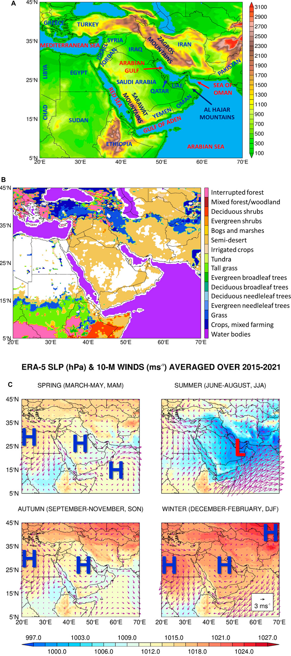
FIGURE 1. Large-Scale Circulation from ERA-5: (A) Topography (m; shading) of the Middle East at 0.25° × 0.25° resolution (∼27 km) from ERA-5. The location of the major countries, water bodies and mountain ranges mentioned in the discussion is highlighted. (B) Predominant vegetation type from ERA-5. Regions devoid of vegetation (desert landscape) are shaded in white. (C) Seasonal-mean sea-level pressure (shading; hPa) and 10-m wind vectors (arrows; m s-1) from ERA-5 averaged over 2015–2021. The predominant anticyclonic and cyclonic systems for each season are highlighted.
Figure 1C summarizes the seasonal-mean large-scale circulation. The main features are: i) the subtropical anticyclones, ubiquitous in the region collocated with the descending branch of the Hadley Cell (Spinks et al., 2015); ii) a thermal low over the eastern Arabian Peninsula in the summer, the Arabian Heat Low (Fonseca et al., 2022); iii) the southwestern extension of the Siberian Anticyclone over southwestern Asia in winter (Hasanean et al., 2013). The low-level flow in the Arabian Sea shifts from southwesterlies in the summer to northeasterlies in winter, in association with the South Asian monsoon circulation (e.g., Schott and McCreary Jr, 2001). The background flow in the Arabian Gulf is north-westerly year-round (Bou Karam Francis et al., 2017; Naizghi and Ouarda, 2017). The region features generally hot and dry weather conditions (e.g., Francis et al., 2020), with air temperatures that can exceed 50°C in the summer when the relative humidity drops below 10% over the desert, while in winter, nighttime temperatures can reach freezing levels and the relative humidity is higher, generally around 60%–80% over coastal regions and above 40% in the desert (Patlakas et al., 2019). There is, however, considerable spatial variability (Hasanean and Almazroui, 2015). In the eastern and southeastern sides, the majority of the annual precipitation, mostly in the range 10–300 mm, falls in the colder months from November to March in association with mid-latitude baroclinic systems (Hasanean and Almazroui, 2015; Wehbe et al., 2017; Wehbe et al. 2018; Wehbe et al. 2020; Nelli et al., 2021). On the western and northwestern sides, the 20–200 mm annual rainfall is mostly driven by the interaction between the Red Sea Trough, a low-pressure trough that extends from equatorial Africa to the eastern Mediterranean and Red Sea, and mid- and upper-level mid-latitude troughs, being more substantial in the autumn (de Vries et al., 2016). Summer convective events occur predominantly i) around the Al Hajar and Sarawat mountains, where they are primarily driven by the interaction of the daytime sea-breeze flow with the topographic circulation and can lead to local accumulations of more than 100 mm of rain (Branch et al., 2020; Francis et al., 2021; Parajuli et al., 2022); ii) in coastal parts of Oman and Yemen, associated with the Asian monsoon (Kwarteng et al., 2009), with more than 400 mm of precipitation on average falling in the mountainous terrain in Yemen in a given year (Hasanean and Almazroui, 2015). Air temperatures are typically in the range 5°C-25°C in winter and 25°C-45°C in the summer, with the northwestern region being the coldest year-round and with the highest temperatures in the Rub’ Al Khali (or Empty Quarter) desert, except in winter where the warmest areas are those bordering the Red Sea (Nelli et al., 2020; Ajjur and Al-Ghamdi, 2021; Nelli et al., 2022). The whole region witnesses frequent dust storms (Francis et al., 2020; Francis et al., 2023a) mostly driven by Shamal winds (Bou Karam Francis et al., 2017), dry cyclones associated with reduced amounts of moisture and clouds but important drivers of dust emission (Bou Karam et al., 2009; Francis et al., 2019a; Francis et al., 2020), density currents from convection (Francis et al., 2019b; Francis et al., 2023a), and cold fronts from mid-latitudes (Kaskaoutis et al., 2019; Nelli et al., 2022).
Figure 2A shows the total CO2 anthropogenic emissions, as given by the EDGARv8 dataset, for 2015 and the difference between 2022 and 2015 expressed as the ratio of the emissions in the 2 years. Further details regarding the major emission sources and their annual cycle are given in Figures 2B,C for the UAE, a country where the emissions are representative of those in the Arabian Peninsula. CO2 emissions in the Middle East have generally remained steady during 2015–2022, partially due to the effects of the COVID-19 pandemic in 2020–2022. There are increases along the main shipping routes in the Arabian Sea and Sea of Oman, in line with the ever booming global trade, and at the location of major oil and gas platforms in the Arabian Gulf, reflecting higher activity. In countries such as Ethiopia and Turkey the anthropogenic emissions in 2022 are slightly larger than in 2015, owing to increased economic development. In Afghanistan and parts of central and southern Sudan, on the other hand, internal conflict has led to an overall decrease in the CO2 anthropogenic emissions. The highest values are concentrated i) around the major cities (e.g., Abu Dhabi in the UAE; Doha in Qatar; Riyadh in Saudi Arabia; Kuwait City in Kuwait); ii) along the main roads and shipping routes; iii) in agricultural-intensive regions, such as the area adjacent to the Nile river and the Nile Delta in Egypt (Awulachew et al., 2012); iv) at the location of oil and gas platforms, as evidenced by the hotspots in the Arabian Gulf (Paris et al., 2021). The narrow orange band extending from the Mediterranean Sea to the Red Sea via the Suez Canal, then into Gulf of Aden, Arabian Sea and further into the Arabian Gulf, is a route commonly taken by ships going from Europe to the countries around the Arabian Gulf (Kaskaoutis et al., 2023).
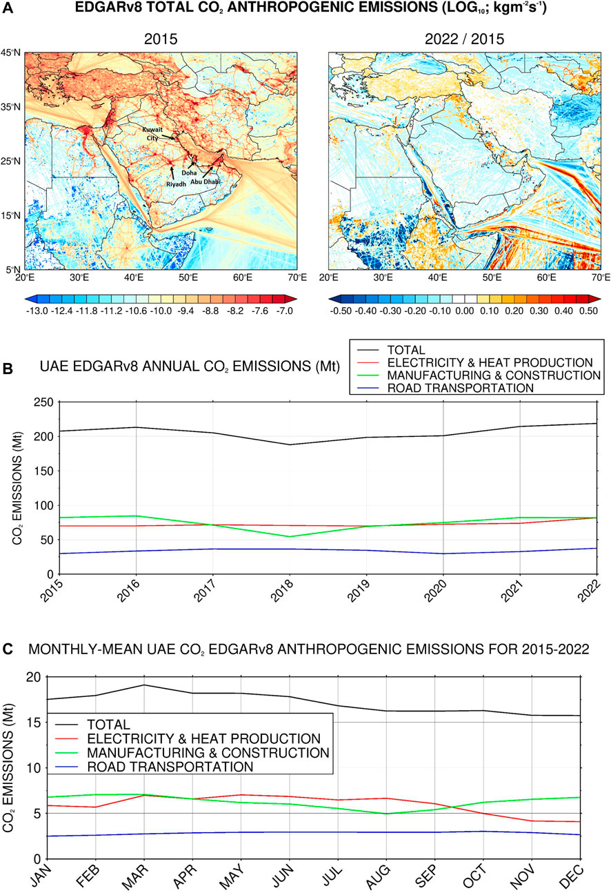
FIGURE 2. CO2 anthropogenic emissions from EDGARv8: (A) Total CO2 emissions (kg m-2 s-1), as given by the EDGARv8 dataset, plotted using a logarithmic scale for easiness of visualization, for 2015 (left) and the ratio between the emissions in 2022 and 2015 (right). White pixels denote missing data, with the location of major cities highlighted in the left panel. (B) UAE CO2 emissions (Megatons, Mt), as given by the EDGARv8 dataset, for 2015–2022. The black line gives the total annual emissions, while the colour lines show the three largest contributors: main activity electricity and heat production (red); manufacturing industries and construction (green); road transportation no resuspension (blue). (C) Is as (b) but giving the monthly-mean emissions averaged over 2015–2022.
The total CO2 emissions in the UAE varied from ∼190 Mt to ∼220 Mt during 2015–2022. As far as the main contributions are concerned, roughly 87%–92% of the emissions come from the energy, manufacturing and construction and transportation sectors, as also noted by Sengul et al. (2009) and Farahat (2016). The drop from 2016 to 2018 is associated with reduced emissions from the manufacturing and construction sectors, which is attributed to decreased investments in light of a fall in oil prices, followed by a rebound in 2018–2019 (Globaldata, 2019). The slight drop in emissions from the transportation sector during 2020 likely reflects the effects of the COVID-19 lockdown. The diversification of energy sources (Ghanem and Alamri, 2023), including the recent opening of the Barakah Power Plant in eastern UAE which does not emit CO2, and investments in renewable energy, explains why, despite a rise in population and manufacturing and construction activity, the CO2 emissions from the energy sector have been declining during 2017–2021, with a slight rebound in 2022. The annual cycle of emissions is given in Figure 2C. While CO2 emissions from the energy sector peak from May to August, likely due to the demand for cooling systems when the air temperatures are the highest (Nelli et al., 2020; 2022), emissions from the manufacturing and construction sectors reach their annual maximum from December to March, as the more extreme summertime weather conditions slow down the activity in those sectors. Given this, the total CO2 emissions in the country peak in March remaining high until June. Emissions from road traffic are roughly constant throughout the year, as most people work year-round, and short-term decreases are offset by an increase in tourists visiting the country.
Even though anthropogenic CO2 emissions generally prevail over natural emissions in arid regions, the latter can still be substantial. For example, Koerner and Klopatek (2002), for the city of Phoenix in Arizona, United States and for the period June 2000 to May 2001, found that roughly 16% of the total annual CO2 emissions came from natural sources (namely, soil respiration), with roughly 80% associated with vehicle emissions. In coastal desert regions, such as the UAE, air-sea fluxes of CO2, which increase with the wind speed (Takahashi et al., 1997; Weiss et al., 2007), also have to be considered. Higher ocean dust deposition leads to a larger CO2 uptake by the ocean and therefore to a decrease in the atmospheric CO2 concentration (Kok et al., 2023). On the other hand, the solubility of atmospheric CO2 into the ocean decreases at warmer temperatures, and hence the atmospheric CO2 concentration will be higher in low-latitude coastal desert regions (Hashimoto, 2019). A quantification of the natural CO2 emissions in the UAE would require the collection of in-situ measurements at several sites that are currently not available in the region.
4 Seasonal CO2 variability and CO2 emissions
The spatial and temporal variability of the XCO2 concentration in the Middle East is summarized in the seasonal mean XCO2 maps given in Figures 3A,B. They are obtained as follows: i) for all OCO-2 and OCO-3 overpasses in the target region, the median (and for the uncertainty the standard deviation) of the XCO2 measurements in each grid-box of the 0.25° × 0.25° ERA-5 grid for a given overpass is estimated; ii) for each grid-box and season, the XCO2 data from all overpasses is averaged to extract the seasonal-mean value. The uncertainty in the XCO2 observations in the study domain is typically of 0.five to one ppmv (Figure 3B). Figure 3C gives the estimated CO2 emission sources and the CO2 transport following the divergence method presented in section 2.2.
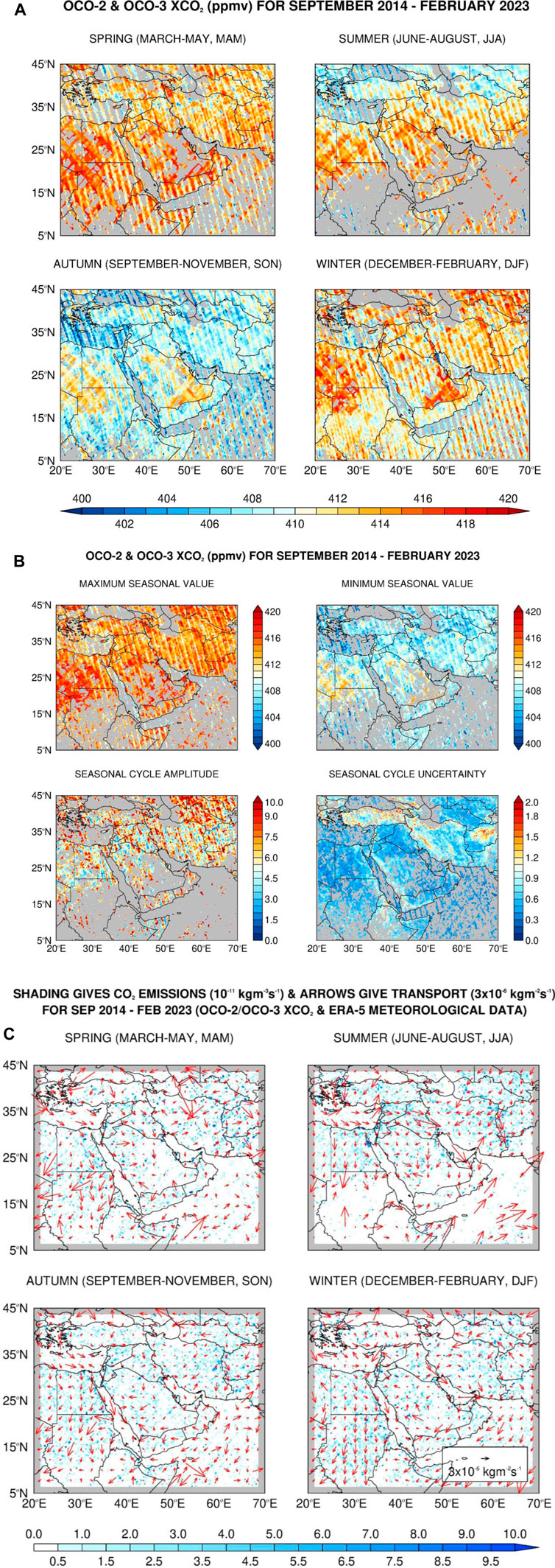
FIGURE 3. Seasonal XCO2 maps and CO2 emissions: (A) Seasonal-mean XCO2 concentration (ppmv) binned in the 0.25° × 0.25° ERA-grid obtained from all OCO-2 overpasses in the period 06 September 2014 to 28 February 2022 and OCO-3 overpasses in the period 06 August 2019 to 28 February 2023. Grey shading denotes regions where no data is available. The maximum and minimum seasonal-mean values, together with the seasonal cycle‘s amplitude and uncertainty are given in (B). (C) The shading gives the CO2 emission (10—11 kg m-3 s-1) and the arrows give the low-level (10-m) transport with respect to the background concentration (3 × 10—6 kg m-2 s-1) obtained with the divergence method detailed in section 2.2. The first five rows/columns are shaded in grey as the background concentration (and hence the emissions) is not defined here.
In general, the XCO2 concentration peaks in spring and reaches its annual minimum in the autumn. This is also the case in Iran using GOSAT data (Golkar and Shirvani, 2020), and over West Asia using OCO-2 data over 2015–2019 (Mustafa et al., 2021). CO2 is a well-mixed gas and its annual variability is largely governed by the seasonal growth in land vegetation (Keeling et al., 1996). In particular, plant growth during the northern hemisphere (where most of the world’s vegetation is found) captures the atmospheric CO2 with a minimum in its concentration in late summer to early autumn, while leaf decay and decomposition and subsequent release of CO2 back to the atmosphere explains the maximum in late winter to early spring. In the UAE, a country which is representative of those in the Arabian Peninsula, the annual maximum occurs in April-May and the minimum in September-October (Figure 4A), when the tropospheric CO2 reaches its annual extremes in the tropics (Crevoisier et al., 2004). Polewards of ∼35°N, on the other hand, the annual maximum occurs in winter and in some parts the lowest annual values are seen in the summer. This region, in particular over Asia, features semi-arid conditions with reduced vegetation coverage, Figure 1B. As a result, anthropogenic emissions play a larger role in the seasonal XCO2 variability, peaking in the winter months when fossil fuel-related energy sources are widely used to heat up buildings (Cao et al., 2017). Around Kuwait, the magnitude of the annual cycle is typically 3–4 ± 0.5 ppmv, Figure 3B, in line with that measured in-situ at Kuwait City from June 1996 to May 2001 (Nasrallah et al., 2003). The seasonal cycle amplitude increases to 8–10 ± 1 ppmv at higher latitudes (Keeling et al., 1996) and in southwestern and southeastern parts of the Arabian Peninsula and tropical Africa (Mengistu and Tsidu, 2020), owing to a more marked seasonality of plant activity on top of anthropogenic emissions in particular in the mid-latitudes (Figure 2A). A similar seasonal cycle amplitude is seen over India where the annual maximum occurs in the drier and hotter pre-monsoon months of April to June, and the minimum in the cooler and wetter summer monsoon months of June to September (Kunchala et al., 2022).
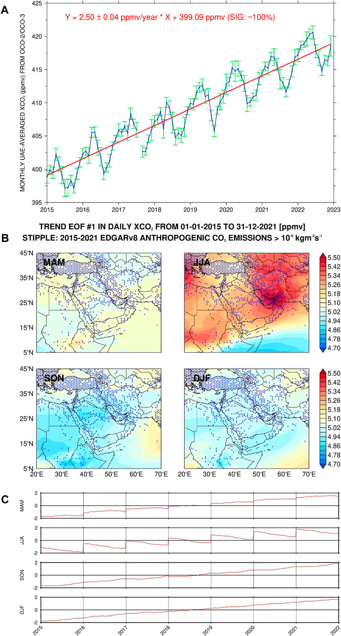
FIGURE 4. Trends in XCO2 concentration: (A) Monthly XCO2 concentration (ppmv; blue line) from the OCO-2/OCO-3 L2 products averaged over the UAE for the period 2015–2022. The red line shows a linear fit to the data with the slope, intercept and statistical significance of the fit provided in the top left. The error bars give one standard deviation from the mean, an indication of the uncertainty in the XCO2 measurements. (B) First Trend EOF (TEOF) of the daily XCO2 concentration (ppmv; shading) for each season and for 2015–2021. Regions where the anthropogenic CO2 emissions, as given by the EDGARv8 dataset and averaged over the same period, exceed 10–9 kg m-2 s-1 are stippled. The first TEOF accounts for between 85% and 99% of variability, while the others represent less than 1% for all seasons. In (C), the respective Trend Principal Components (TPCs) are plotted. The gridded OCO-2 L3 product is used for the TEOF analysis.
In addition to heterogeneity in terms of the temporal variability, there are also differences in the spatial pattern of the XCO2 concentration. The spatial variations can be understood by looking at the CO2 emissions and CO2 transport with respect to the background concentration given in Figure 3C, estimated using the divergence method summarized in Section 2.2. It is interesting to note that the magnitude of the CO2 transport, typically in the range 10–7 to 10–5 kg m-2s-1, is comparable to some of the largest anthropogenic emissions as given by the EDGARv8 dataset (Figure 2A). This stresses the role played by the horizontal advection of CO2 in the spatial distribution of the XCO2 concentration (cf. Figures 3A,B), even though the inversion technique may be over-predicting the CO2 fluxes (Deng et al., 2022). The hotspots in parts of Libya, Egypt and northern Chad and Sudan as well as in southeastern Saudi Arabia over the Rub’ Al Khali desert in the autumn and winter are driven both by the transport of CO2 and emission sources (Figure 3C), the latter playing the largest role in northeastern Africa. Here, the magnitude of the estimated CO2 emissions is largely comparable to that of the anthropogenic ones given in Figure 2A, suggesting biogenic emissions likely play a reduced role, which is consistent with the semi-arid landscape (Figure 1B). The clear contrast in the number of CO2 emission sources over tropical Africa between the summer, when they are largely absent, and the winter season, when they are abundant, is consistent with the fact that during the wet (summer) months the vegetation (Figure 1B) picks up CO2 from the atmosphere, with very little transport as the low-level flow is from the southwest (Figures 1C, 3C). This explains the lower XCO2 concentrations seen here in the warmer months (blue patches in Figure 3A). The downstream transport of CO2 (Figure 3C), combined with reduced emission sources over the eastern Mediterranean where forests are present year-round (Figure 1B), is in line with the lower XCO2 values here throughout the year (Figures 3A,B). A visual comparison of the CO2 emission sources in Figure 3C with the CO2 anthropogenic emissions given by the EDGARv8 dataset in Figure 2A reveals that the latter play an important role: e.g., the higher number of sources along the Nile River in Egypt, in coastal areas around the Arabian Gulf, and around Israel, Jordan and Syria together with the dearth of emission sources over tropical Africa between 5° and 15° N in particular in the warmer months are present in both maps. There are, however, some important differences. Given that the two products have different spatial resolutions (0.1° for EDGARv8 and 0.25° for the estimated CO2 emissions), in regions of complex topography the divergence method will not be able to capture localized emission sources such as those in western and southwestern Iran, around the Sarawat mountains in Yemen and Saudi Arabia, and over parts of Turkey. The signal from transient emission sources such as ships seen in Figure 2A is also not present in Figure 3C. An evaluation of the magnitudes of the estimated emissions (Figure 3C) against the anthropogenic ones (Figure 2A) reveals they tend to be largely similar in regions that feature a lack of vegetation (cf. Figure 1B), with the former exceeding the latter in vegetated regions. The comparison of the seasonal-mean XCO2 concentrations in Figures 3A,B with the CO2 emission sources and transport in Figure 3C and the anthropogenic emissions as given by the EDGARv8 dataset (Figure 2A) sheds light on some of the processes behind the spatial and temporal variability of the satellite-derived XCO2 data.
5 Trends in CO2 concentration
Having discussed the seasonal variability in XCO2, the trend will now be examined. Figure 4A shows the monthly UAE-averaged XCO2 for 2015–2022. This plot is obtained as follows: i) for each OCO-2 and OCO-3 overpass, the median (and for the uncertainty the standard deviation) of the XCO2 measurements in the 0.25° × 0.25° grid used by ERA-5 at a given overpass is estimated; ii) for each month in the period 2015–2022, the XCO2 data at each grid-box is averaged over all overpasses; iii) all XCO2 data points in the grid-boxes inside the UAE are averaged for each month. It is important to note that all measurements, regardless of their quality flag value, are considered to generate Figure 4A. If only good quality retrievals are used, the overall findings are similar but there are far more gaps in the time-series (not shown).
On top of the annual variability, there is a marked positive trend in the monthly data for the 8-year period at a rate of about 2.50 ± 0.4 ppmv/year, statistically significant at the 95% confidence level. The magnitude of the trend is on the higher side of the 1.8–2.2 ppmv/year estimated for different regions of the world (Kuttippurath et al., 2022). However, even steeper trends have been measured such as an OCO-2 trend of 2.8 ppmv/year over India from July 2014 to December 2018 (Kunchala et al., 2022), and a GOSAT-derived trend of 2.6 ± 0.3 ppmv/year over the Arctic Ocean for July-September 2009–2016 (Payan et al., 2017). The trend reported here for the UAE is steeper than the 1.92 to 2.16 ppmv/year estimated over Iran for May 2009 - June 2016 using GOSAT data (Golkar and Shirvani, 2020), and the 2.1 ppmv/year for the same region using GOSAT and Environmental Satellite (ENVISAT) data for the period 2003–2015 (Safaeian et al., 2023). The fact that the period over which the trend is computed in this study (namely, 2015–2022) includes more recent years when the rise in the CO2 concentration has become steeper (Tans and Keeling, 2023), and the biases in the satellite-derived estimates which, as noted by Kuttippurath et al. (2022), can be substantial, may explain the higher trend magnitude compared to that reported elsewhere. CO2 trends estimated using in-situ measurements are comparable to these: e.g., Jain et al. (2021) estimated a trend of 2.5 ± 1.2 ppmv/year from surface measurements in southern India for the period April 2016 to April 2019, while Imasu and Tanabe (2018) reported a trend of about 2 ppmv/year for urban, suburban and rural areas around Tokyo. The fact that the CO2 trends from different locations and obtained with ground-based and satellite assets have a similar magnitude in the range 1.8–2.6 ppmv/year is explained by the fact that CO2 is a well-mixed gas (Kuttippurath et al., 2022).
In order to gain further insight into the XCO2 variability, the TEOF technique is applied to the OCO-2 daily L3 gridded product. Figure 4B gives the first TEOF for each season, which represents 85%–99% of the variability (not shown), with the TPCs shown in Figure 4C. It is important to note that here the trends are being examined, and their spatial and temporal patterns do not necessarily have to match those of the seasonal-mean XCO2 concentration given in Figure 3A. The largest trend values are seen in the summer when the highest surface and air temperatures occur (e.g., Alizadeh and Babei, 2022), which promote soil respiration and organic matter decomposition (Raich et al., 2002; Knorr et al., 2005) and reduce the solubility of the CO2 into the ocean (Hashimoto, 2019). There is a hospot over northeastern UAE and southern Iran in this season, which largely overlaps with the region of higher anthropogenic emissions as given by the EDGARv8 dataset (cf. Figure 2A). The accumulation of emissions over this area during summer can also arise due to the convergence of three wind regimes: Shamal winds from the northwest, monsoon flow from the southwest and the Levar winds from the northeast (e.g., Rashki et al., 2019; Francis et al., 2020).
The lower values over the equatorial Indian Ocean and eastern Africa coincide with a region of reduced CO2 emissions (cf. Figures 2A, 3C), and where the extension into higher latitudes is consistent with the northward transport of CO2 in this season (Figure 3C). Over tropical Africa, the highest trend values in the summer (wet) season are mostly driven by deforestation (cf. Figure 1B) and subsequent release of CO2 into the atmosphere (Baccini et al., 2012; Salih et al., 2013; Duku and Hein, 2021). For the other seasons the spatial variability is much smaller, generally within 5%–10%.
The TPCs given in Figure 4C show a steady increase in the 7-year period, in line with the upward trend in CO2 concentrations over the UAE estimated from the L2 orbital retrievals, Figure 4A. There are, however, marked differences in the intra-seasonal variability: there is a clear increase in autumn and winter, a slight increase in spring, and a decrease in the summer. For the vast majority of the countries in the region, anthropogenic emissions peak in the winter months (e.g., Figures 2C, 3C). The rise in the cold season emissions in the period 2015–2021 is likely tied to higher fossil fuel burning to heat up buildings over a backdrop of a rising population. The steady increase during the winter months seen in the respective TPC may be attributed to the fact that the coldest temperatures normally occur in January and February, and therefore at the end of the season. A similar reasoning can explain the variability in the autumn, with the TPC values rising gradually at the beginning and then faster at the end when the weather starts to turn colder. Natural variability is likely at play as well, as the demise of the vegetation is gradual meaning that earlier in the season the plants are still able to remove CO2 from the atmosphere through photosynthesis. The fact that the reduction in anthropogenic emissions and the growth in vegetation reach the maximum in this season likely explain the decreasing values during the summer, with a more muted intra-seasonal variability in spring. It is interesting to note that, while in the autumn and winter there is a smooth transition from 1 year to the next, in spring, and in particular in summer, there is a jump or a step in the time-series. This is also seen in the raw data (not shown), and is a consequence of the weak (in spring) and decreasing (in summer) intra-seasonal variations over a background of rising concentrations. In autumn and winter the increasing values during the season have the same sign as the trend in the background concentration, which is also increasing over time, yielding a smoother time-series.
6 Comparison of OCO with CO2 forcing data in climate change simulations
In this section, the CO2 concentrations used as input in (and not a prediction of) the CMIP6 climate change simulations are evaluated against the OCO-2/OCO-3 measurements. The historical period is 1850–2014, and therefore does not overlap with the OCO data that extends from 2015 to 2022. Hence, the comparison will be done for the first 8 years of the climate change period, 2015–2022, when both are available. The satellite-derived data used here is obtained as follows: i) for each OCO-2 and OCO-3 overpass in the period 2015 to 2022, and for the same 0.5° latitude grid used in the CO2 forcing data, the median of the XCO2 measurements for all longitudes for a given overpass is obtained; ii) the latitudinal XCO2 values for each month in the 8-year period are averaged over all overpasses.
Figures 5A,B show a time-series of the CO2 concentration from OCO-2/OCO-3 (black) and eight SSP scenarios averaged over 05.25°-15.25°N and 35.25°-45.25°N, respectively, which are representative of the southern and northern parts of the target domain. In the deep tropics, Figure 5A, for 2015 and 2016 the OCO and the forcing data’s CO2 are roughly in agreement, even though the amplitude of the seasonal cycle is about two times larger in the latter. For 2017–2022, there is a clear positive bias in the forcing data, whose rate of increase is roughly 10%–30% higher than that of the observed, suggesting that in all five scenarios, and for this range of latitudes, the forcing data overestimates the amount of CO2 in the atmosphere and therefore its impact on the Earth’s climate. While in 2015–2018 there is little variability between the different scenarios, by 2019–2022 there is a clear distinction between them, with lower values for SSP1 and higher for SSP3 and SSP5 by up to about 2 ppmv, with the differences amplifying over time. This is expected, as the scenarios are initialized in 2015 and it takes some time for the increased emissions in SSP3-5 compared to SSP1-2 to be felt in the column concentrations. The differences are even more marked in the mid-latitudes, Figure 5B, with the latitude range 35.25°-45.25°N comprising major urban centers and industrial activities where CO2 emissions are likely to rise more strongly. The year-on-year increase in the forcing CO2 data is up to 30% larger than that in OCO, with positive biases reaching up to 12 ppmv by 2022 and a twice as large seasonal cycle amplitude. The increase in the seasonality of the CO2 annual cycle has been observed in recent decades and is estimated to be as much as 50% in the last 50 years in the Northern Hemisphere. It has been attributed to a rise in the ecosystems and croplands’ productivity (Gray et al., 2014; Forkel et al., 2016), and is projected to continue to increase in the future, with a doubling of its amplitude by 2,100 in the SSP5-8.5 scenario (Meinshausen et al., 2020). In addition, the fact that the CO2 forcing data is originally a surface mole fraction is also consistent with the higher seasonality with respect to the satellite-derived XCO2 concentration.
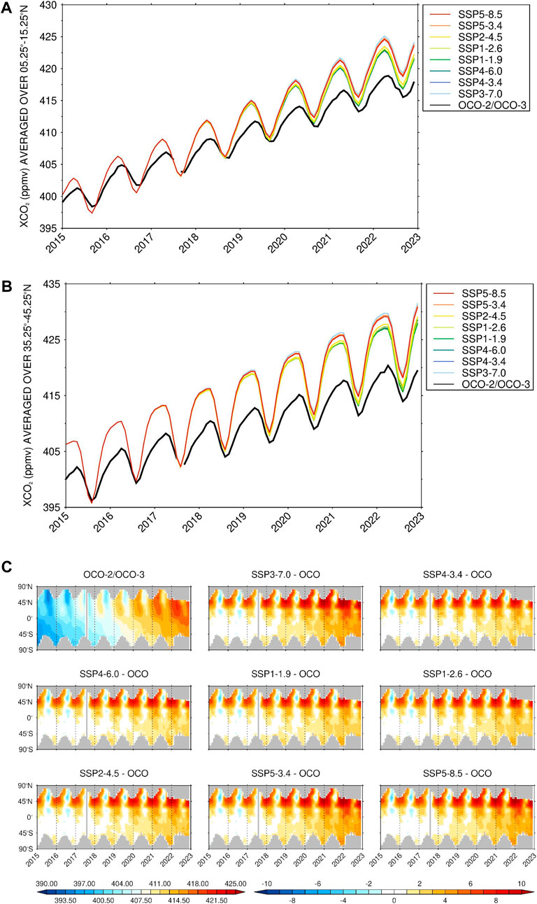
FIGURE 5. Comparison of OCO with CO2 forcing data in future climate simulations: Monthly XCO2 concentration (ppmv) averaged over (A) 05.25°-15.25°N and (B) 35.25°-45.25°N from OCO-2/OCO-3 (black line) and that given by eight different shared socioeconomic pathway (SSP) scenarios from 2015 to 2022. (C) Hovmoller plot of monthly XCO2 from OCO-2/OCO-3 (top left) and the difference with respect to that of the eight SSP scenarios (remaining plots) for 2015 to 2022. Grey shading indicates no data from the satellite-derived product.
Further insight can be gained by looking at the full dataset (Figure 5C). The first panel shows OCO-2/OCO-3 data, which exhibits a marked annual cycle in the Northern Hemisphere and a much reduced one in the Southern Hemisphere due to lower amounts of vegetation and where oceans prevail in the mid-latitudes and ice is dominant at higher latitudes (Cleveland et al., 1983). On top of this there is a gradual increase in magnitude over the 8-year period, with the phase remaining largely unchanged. The OCO-2/OCO-3 estimated XCO2 is qualitatively similar to that estimated from other satellites’ measurements (Jiang et al., 2016). The other panels in Figure 5C show the differences with respect to the OCO data for each of the eight climate change scenarios. In the Southern Hemisphere the discrepancy is rather small but the CO2 is still overestimated, with biases in the range 0–2 ppmv increasing to 5 ppmv at higher latitudes by 2022. However, in the Northern Hemisphere the differences are pronounced, exceeding 10 ppmv by 2022 in particular around 40-50°N, roughly the latitude of the major urban centers and energy-producing regions in the world. The higher CO2 amounts in the Northern Hemisphere are generally in phase with the seasonal cycle, acting to increase its amplitude, with slight negative values in summer and autumn and much larger positive values in winter and spring. As also seen in the time-series in Figures 5A,B, the difference in CO2 between the scenarios is generally small in 2015–2021, but more recently, and in particular in 2022, the column concentrations in SSP5-8.5 are at times more than 3 ppmv higher than those in SSP1-1.9.
The results in Figure 5 indicate that the CO2 concentration used to drive climate change models is likely overestimated, which has implications for the interpretation of their predictions. Gurriaran et al. (2023) developed a model to estimate the demand for electricity in Qatar until the end of the century driven by the temperature projections from CMIP6 models. They found an average rate of increase of +4.2%/°C for the electricity demand, projected to rise by 5%–35% due to warming alone by 2,100. An accurate input of CO2 concentrations is therefore needed to improve the reliability of future climate projections.
7 Discussion and conclusion
Carbon dioxide (CO2) is the most prominent anthropogenic greenhouse gas and its concentration has been rising in recent decades at an ever-increasing rate (Quadrelli and Peterson, 2007; Tans and Keeling, 2023). Despite its crucial role in the Earth’s climate (Feldman et al., 2015), there are still only a few ground-based CO2 measurements worldwide (Wunch et al., 2011a), and none in the Middle East, which is an emission hotspot (Mustafa et al., 2021; Francis et al., 2023b). The variability in the column CO2 (XCO2) concentration, as given by the measurements collected by the Orbiting Carbon Observatory-2 (OCO-2) and OCO-3 in the period September 2014 to February 2023, and its trends in the Middle East are analyzed in this work. They are also used to assess the CO2 data ingested into future climate simulations for different climate change scenarios. The central goals of this work are to i) shed light on the current state of the CO2 concentrations ii) identify areas and seasons where it has been increasing at a faster rate and where in-situ measurements would be more valuable; iii) evaluate the CO2 data used to drive climate change simulations against satellite-derived measurements. The findings of this study will help in the development of adaptation and mitigation strategies aiming at reducing emissions and ensuring a more sustainable future.
The XCO2 concentration generally peaks in spring and reaches its annual minimum in the autumn, in line with the seasonal cycle of land vegetation (Keeling et al., 1996). In the Arabian Peninsula, the annual cycle amplitude is typically 3–8 ± 0.5 ppmv increasing to 8–10 ± 1 ppmv in the mid-latitudes. The spatial variability in the seasonal-mean XCO2 concentration can be at least partially explained by the CO2 emissions and transport, such as the hotspots over Libya, Egypt and northern Chad and Sudan and over southeastern Saudi Arabia in autumn and winter. A comparison with an anthropogenic CO2 emission inventory indicated anthropogenic sources play an important role in the spatial distribution of the XCO2 concentration, in particular in arid and semi-arid regions largely devoid of vegetation. The trend in the XCO2 values over the UAE for 2015–2022 is estimated to be 2.50 ± 0.4 ppmv/year, slightly higher than that reported at other sites in the Middle East (e.g., Golkar and Shirvani, 2020) but slightly lower than that estimated over India in the recent years (Kunchala et al., 2022). This has been attributed to biases in the satellite-derived estimates (Kuttippurath et al., 2022) and to the fact that more recent years have been considered in the analysis, when the CO2 concentration has increased at a faster rate. In any case, even steeper trends have been reported elsewhere using satellite and ground-based measurements, and the UAE is regarded as a hotspot in CO2 emissions inventories. A statistical analysis of the gridded OCO-2 level 3 product revealed a trend hotspot over northeastern UAE in the summer, in an area of increased anthropogenic emissions and low-level wind convergence.
An evaluation of the CO2 data used to drive climate change simulations, for which OCO-2 and OCO-3 measurements are not considered, against the satellite-derived values revealed an overestimation of the former, with a magnitude exceeding 10 ppmv in particular between 40° and 50°N where the major urban centers are located. The trend in the XCO2 increase in the forcing data is up to 30% steeper than that in the OCO measurements, with the amplitude of its seasonal cycle also increasing faster than in observations, being twice as large by 2022. This is a reflection of the premises made with respect to the latitudinal gradients and seasonality when generating the CO2 forcing data, as well as the assumption that the CO2 surface mole fraction is propagated vertically in the models so it can be directly compared to the satellite-derived XCO2 concentration (Meinshausen et al., 2020). As CO2 acts to generally warm the surface and the atmosphere, this suggests the projected temperature changes over the Arabian Peninsula may be overestimated, which can be further amplified by the deficiencies in the models’ physics and dynamics.
Further insight into the CO2 variability can be gained through higher spatial and temporal frequency data. This can be achieved by a comprehensive network of ground-based observations, which is still lacking to date in the Arabian Peninsula, and/or through more sophisticated satellites such as the three planned to be launched in 2025 as part of the European Space Agency’s CO2 Monitoring (CO2M) mission (Sierk et al., 2021). Such observations are also crucial for the evaluation of the performance of numerical models, and subsequently improve the quality of their forecasts for both the current and future climate. In addition, measurements at different heights collected by aircraft (Tanaka et al., 2012), tethered balloons (Li et al., 2014), and/or drones are needed to understand the vertical structure of the CO2 concentration and estimate, for this region, the typical vertical mixing time-scale, which is a function of the three dimensional atmospheric circulation (e.g., Babu et al., 2023).
8 Research data
The following datasets are employed in this study: i) three products from the Orbiting Carbon Observatory (OCO): OCO-2 and OCO-3 level 2 data (Gunson and Eldering, 2020; Chatterjee and Payne, 2022) and OCO-2 level 3 data (Weir and Ott, 2022); ii) CO2 emissions from the Emissions Database for Global Atmospheric Research version 8.0, available on the European Commission’s website (European Commission, 2023); iii) ERA-5 pressure-level (Hersbach et al., 2018a; 2019b) and surface (Hersbach et al., 2018b; 2019a) reanalysis data; iv) CO2 data used to drive the future climate simulations of five models of the Coupled Model Intercomparison Project 6 (CMIP6; University of Melbourne, 2023; ESGF, 2023). All figures were generated using the Interactive Data Language (Bowman, 2005) software version 8.8.1.
Data availability statement
The raw data supporting the conclusions of this article will be made available by the authors, without undue reservation.
Author contributions
RF: Data curation, Formal Analysis, Investigation, Methodology, Validation, Visualization, Writing–original draft. DF: Conceptualization, Funding acquisition, Investigation, Project administration, Resources, Supervision, Validation, Writing–review and editing.
Funding
The author(s) declare that no financial support was received for the research, authorship, and/or publication of this article.
Acknowledgments
We would like to acknowledge the contribution of Khalifa University’s high-performance computing and research computing facilities to the results of this research. The OCO-2 and OCO-3 data used in this work were produced by the OCO project at the Jet Propulsion Laboratory, California Institute of Technology, and was obtained from the OCO data archive maintained at the NASA Goddard Earth Science Data and Information Services Center. We would like to thank the editor and the two reviewers for their several comments and suggestions that helped to significantly improve the quality of this manuscript.
Conflict of interest
The authors declare that the research was conducted in the absence of any commercial or financial relationships that could be construed as a potential conflict of interest.
Publisher’s note
All claims expressed in this article are solely those of the authors and do not necessarily represent those of their affiliated organizations, or those of the publisher, the editors and the reviewers. Any product that may be evaluated in this article, or claim that may be made by its manufacturer, is not guaranteed or endorsed by the publisher.
References
Ajjur, S. B., and Al-Ghamdi, S. G. (2021). Seventy-year disruption of seasons characteristics in the Arabian Peninsula. Int. J. Climatol. 41, 5920–5937. doi:10.1002/joc.7160
Alizadeh, O., and Babaei, M. (2022). Seasonally dependent precipitation changes and their driving mechanisms in Southwest Asia. Clim. Change 171, 20. doi:10.1007/s10584-022-03316-z
Al Senafi, F., Anis, A., and Menezes, V. (2019). Surface heat fluxes over the northern arabian Gulf and the northern Red Sea: evaluation of ECMWF-ERA5 and NASA-MERRA2 reanalyses. Atmosphere 10, 504. doi:10.3390/atmos10090504
Ambaum, M. H. P. (2010). Thermal physics of the atmosphere. John Wiley and Sons Ltd, 239. 9780470710364. Print ISBN: 9780470745151. Online. doi:10.1002/9780470710364
Arman, H. (2015). Uncertainties, risks and challenges relating to CO2 emissions and its possible impact on climate change in the United Arab Emirates. Int. J. Glob. Warming 8, 1–17. doi:10.1504/IJGW.2015.071575
Arshad, M., Ma, X., Yin, J., Ullah, W., Liu, M., and Ullah, I. (2021). Performance evaluation of ERA-5, JRA-55, MERRA-2, and CFS-2 reanalysis datasets, over diverse climate regions of Pakistan. Weather Clim. Extrem. 33, 100373. doi:10.1016/j.wace.2021.100373
Aumann, H. H., Gregorich, D., and Gaiser, S. (2005). AIRS hyper-spectral measurements for climate research: carbon dioxide and nitrous oxide effects. Geophys. Res. Lett. 32, L05806. doi:10.1029/2004GL021784
Awulachew, S. B., Smakhtin, V., Molden, D., and Peden, D. (2012). The Nile River basin: water, agriculture, governance and livelihoods. New York, NY, United States: Routledge, Taylor and Francis Group, 321.
Babu, R., Ou-Yang, C.-F., Griffith, S. M., Pani, S. K., Kong, S. S.-K., and Lin, N. H. (2023). Transport pathways of carbon monoxide from Indonesian fire pollution to a subtropical high-altitude mountain site in the western North Pacific. Atmos. Chem. Phys. 23, 4727–4740. doi:10.5194/acp-23-4727-2023
Baccini, A., Goetz, S. J., Walker, W. S., Laporte, N. T., Sun, M., Sulla-Menashe, D., et al. (2012). Estimated carbon dioxide emissions from tropical deforestation improved by carbon-density maps. Nat. Clim. Change 2, 182–185. doi:10.1038/nclimate1354
Ballantyne, A. P., Alden, C. B., Miller, J. B., Tans, P. P., and White, J. W. C. (2012). Increase in observed net carbon dioxide uptake by land and oceans during the past 50 years. Nature 488, 70–72. doi:10.1038/nature11299
Barbosa, S. M., and Andersen, O. B. (2009). Trend patterns in global sea surface temperature. Int. J. Climatol. 29, 2049–2055. doi:10.1002/joc.1855
Bell, E., O’Dell, C. W., Taylor, T. E., Merrelli, A., Nelson, R. R., Kiel, M., et al. (2023). Exploring bias in the OCO-3 snapshot area mapping mode via geometry, surface, and aerosol effects. Atmos. Meas. Tech. 16, 109–133. doi:10.5194/amt-16-109-2023
Boesch, H., Bake, D., Connor, B., Crisp, D., and Miller, C. (2011). Global characterization of CO2 column retrievals from shortwave-infrared satellite observations of the orbiting carbon observatory-2 mission. Remote Sens. 3, 270–304. doi:10.3390/rs3020270
Boucher, O., Borella, A., Gasser, T., and Hauglustaine, D. (2021). On the contribution of global aviation to the CO2 radiative forcing of climate. Atmos. Environ. 267, 118762. doi:10.1016/j.atmosenv.2021.118762
Bou Karam, D., Flamant, C., Tulet, P., Todd, M. C., Pelon, J., and Williams, E. (2009). Dry cyclogenesis and dust mobilization in the intertropical discontinuity of the West African Monsoon: a case study. J. Geophys. Res. 114, D05115. doi:10.1029/2008JD010952
Bou Karam Francis, D., Flamant, C., Chaboureau, J.-P., Banks, J., Cuesta, J., Brindley, H., et al. (2017). Dust emission and transport over Iraq associated with the summer Shamal winds. Aeolian Res. 24, 15–31. doi:10.1016/j.aeolia.2016.11.001
Bowman, K. P. (2005). An introduction to programming with IDL: interactive Data Language [software]. Academic Press, 304. ISBN-10: 012088559X, ISBN-13: 978-0120885596.
Branch, P., Behrendt, A., Gong, Z., Schwitalla, T., and Wulfmeyer, V. (2020). Convection initiation over the eastern arabian Peninsula. Meteorol. Z. 29, 67–77. doi:10.1127/metz/2019/0997
Cao, L., Chen, X., Zhang, C., Kurban, A., Yuan, X., Pan, T., et al. (2017). The temporal and spatial distributions of the near-surface CO2 concentrations in central Asia and analysis of their controlling factors. Atmosphere 8, 85. doi:10.3390/atmos8050085
Ceron, W. L., Andreoli, R. V., Kayano, M. T., Canchala, T., Ocampo-Marulanda, C., Avila-Diaz, A., et al. (2022). Trend pattern of heavy and intense rainfall events in Colombia from 1981-2018: a trend-EOF approach. Atmosphere 13, 156. doi:10.3390/atmos13020156
Chatterjee, A., and Payne, V. (2022). OCO-3 Level 2 bias-corrected XCO2 and other select fields from the full-physics retrieval aggregated as daily files. Retrospective processing v10.4r [Dataset]. Greenbelt, MD, USA: Goddard Earth Sciences Data and Information Services Center (GES DISC). doi:10.5067/970BCC4DHH24Accessed on May 15, 2023)
Chen, Z., Jacob, D. J., Nesser, H., Sulprizio, M. P., Lorente, A., Varon, D. J., et al. (2022). Methane emissions from China: a high-resolution inversion of TROPOMI satellite observations. Atmos. Chem. Phys. 22, 10809–10826. doi:10.5194/acp-22-10809-2022
Cheng, Y., Shan, Y., Xue, Y., Zhu, Y., Wang, X., Xue, L., et al. (2022). Variation characteristics of atmospheric methane and carbon dioxide in summertime at a coastal site in the South China Sea. Front. Environ. Sci. Eng. 16, 139. doi:10.1007/s11783-022-1574-z
Cleveland, M. S., Freeny, A. E., and Graedel, T. E. (1983). The seasonal component of atmospheric CO2: information from new approaches to the decomposition of seasonal time series. J. Geophys. Res. 88, 10934–10946. doi:10.1029/JC088iC15p10934
Crawford, B., Christen, A., and McKendry, I. (2016). Diurnal course of carbon dioxide mixing ratios in the urban boundary layer in response to surface emissions. J. Appl. Meteorology Climatol. 55, 507–529. doi:10.1175/JAMC-D-15-0060.1
Crevoisier, C., Heilliette, S., Chedin, A., Serrar, S., Armante, R., and Scott, N. A. (2004). Midtropospheric CO2 concentration retrieval from AIRS observations in the tropics. Geophys. Res. Lett. 31, L17106. doi:10.1029/2004gl020141
Crippa, M., Guizzardi, D., Pagani, F., Banja, M., Muntean, M., Schaaf, E., et al. (2023). GHG emissions of all world countries. Luxembourg: Publications Office of the European Union, JRC134504. doi:10.2760/953322
Crisp, D., Fisher, B. M., O’Dell, C., Frankenberg, C., Basilio, R., Bosch, H., et al. (2012). The ACOS CO&lt;sub&gt;2&lt;/sub&gt; retrieval algorithm – Part II: global X&lt;sub&gt;CO&lt;sub&gt;2&lt;/sub&gt;</sub&gt; data characterization. Atmos. Meas. Tech. 5, 687–707. doi:10.5194/amt-5-687-2012
Cristofanelli, P., Calzolari, F., Bonafe, U., Lanconelli, C., Lupi, A., Busetto, M., et al. (2011). Five-year analysis of background carbon dioxide and ozone variations during summer seasons at the Mario Zucchelli station (Antarctica). Tellus B 63, 831–842. doi:10.1111/j.1600-0889.2011.00576.x
Das, C., Kunchala, R. K., Chandra, N., Chmura, L., Necki, J., and Patra, P. K. (2022). Meridional propagation of carbon dioxide (CO2) growth rate and flux anomalies from the tropics due to ENSO. Geophys. Res. Lett. 49, e2022GL100105. doi:10.1029/2022GL100105
Dasari, H. P., Viswanadhapalli, Y., Langodan, S., Abualnaja, Y., Desamsetti, S., Vankayalapati, K., et al. (2022). High-resolution climate characteristics of the Arabian Gulf based on a validated regional reanalysis. Meteorol. Appl. 29, e2102. doi:10.1002/met.2102
Deng, Z., Ciais, P., Tzompa-Sosa, Z. A., Saunois, M., Qiu, C., Tan, C., et al. (2022). Comparing national greenhouse gas budgets reported in UNFCCC inventories against atmospheric inversions. Earth Syst. Sci. Data 14, 1639–1675. doi:10.5194/essd-14-1639-2022
de Vries, A. J., Feldstein, S. B., Riemer, M., Tyrlis, E., Sprenger, M., Baumgart, M., et al. (2016). Dynamics of tropical-extratropical interactions and extreme precipitation events in Saudi Arabia in autumn, winter and spring. Q. J. R. Meteorological Soc. 142, 1862–1880. doi:10.1002/qj.2781
Dhakal, S., Minx, J. C., Toth, F. L., Abdel-Aziz, A., Figueroa Meza, M. J., Hubacek, K., et al. (2022). “Emissions trends and drivers,” in IPCC, 2022: climate change 2022: mitigation of climate change. Contribution of working group III to the sixth assessment report of the intergovernmental panel on climate change. Editors P. R. Shukla, J. Skea, R. Slade, A. Al Khourdajie, R. van Diemen, D. McCollumet al. (Cambridge, UK and New York, NY, USA: Cambridge University Press). doi:10.1017/9781009157926.004
Duku, C., and Hein, L. (2021). The impact of deforestation on rainfall in Africa: a data-driven assessment. Environ. Res. Lett. 16, 064044. doi:10.1088/1748-9326/abfcfb
Eldering, A., Taylor, T. E., O’Dell, C. W., and Pavlick, R. (2019). The OCO-3 mission: measurement objectives and expected performance based on 1 year of simulated data. Atmos. Meas. Tech. 12, 2341–2370. doi:10.5194/amt-12-2341-2019
EPA (2023). Overview of greenhouse gases. available online at https://www.epa.gov/ghgemissions/overview-greenhouse-gases#carbon-dioxide (Accessed on February 23, 2023).
ESGF (2023). World climate research project (WCRP) coupled model Intercomparison project 6 (CMIP6) [dataset]. Earth System Grid Federation. available online at https://esgf-node.llnl.gov/projects/cmip6/ (Accessed on February 07, 2023).
European Commission (2023). Emissions Database for global atmospheric research version 8 .0 [dataset]. available online at https://edgar.jrc.ec.europa.eu/dataset_ghg (Accessed on October 30, 2023).
Eyring, V., Bony, S., Meehl, G. A., Senior, C. A., Stevens, B., Stouffer, R. J., et al. (2016). Overview of the coupled model Intercomparison project phase 6 (CMIP6) experimental design and organization. Geosci. Model Dev. 9, 1937–1958. doi:10.5194/gmd-9-1937-2016
Farahat, A. (2016). Air pollution in the Arabian Peninsula (Saudi Arabia, the United Arab Emirates, Kuwait, Qatar, Bahrain, and Oman): causes, effects, and aerosol categorization. Arabian J. Geosciences 9, 196. doi:10.1007/s12517-015-2203-y
Feldman, D., Collins, W., Gero, P., Torn, M. S., Mlawer, E. J., and Shippert, T. R. (2015). Observational determination of surface radiative forcing by CO2 from 2000 to 2010. Nature 519, 339–343. doi:10.1038/nature14240
Fonseca, R., Francis, D., Nelli, N., and Thota, M. (2022). Climatology of the heat low and the intertropical discontinuity in the Arabian Peninsula. Int. J. Climatol. 42, 1092–1117. doi:10.1002/joc.7291
Forkel, M., Carvalhais, N., Rodenbeck, C., Keeling, R., Heimann, M., Thonicke, K., et al. (2016). Enhanced seasonal CO2 exchange caused by amplified plant productivity in northern ecosystems. Science 351, 696–699. doi:10.1126/science.aac4971
Francis, D., Alshamsi, N., Cuesta, J., Isik, A. G., and Dundar, C. (2019a). Cyclogenesis and density currents in the Middle East and the associated dust activity in september 2015. Geosciences 9, 376. doi:10.3390/geosciences9090376
Francis, D., Chaboureau, J.-P., Nelli, N., Cuesta, J., Alshamsi, N., Temimi, M., et al. (2020). Summertime dust storms over the Arabian Peninsula and impacts on radiation, circulation, cloud development and rain. Atmos. Res. 250, 105364. doi:10.1016/j.atmosres.2020.105364
Francis, D., Fonseca, R., Nelli, N., Bozkurt, D., Cuesta, J., and Bosc, E. (2023a). On the Middle East's severe dust storms in spring 2022: triggers and impacts. Atmos. Environ. 296, 119539. doi:10.1016/j.atmosenv.2022.119539
Francis, D., Fonseca, R., Nelli, N., Teixido, O., Mohamed, R., and Perry, R. (2019b). Increased Shamal winds and dust activity over the Arabian Peninsula during the COVID-19 lockdown period in 2020. Aeolian Res. 55, 100786. doi:10.1016/j.aeolia.2022.100786
Francis, D., Temimi, M., Fonseca, R., Nelli, N. R., Abida, R., Weston, M., et al. (2021). On the analysis of a summertime convective event in a hyperarid environment. Q. J. R. Meteorological Soc. 147, 501–525. doi:10.1002/qj.3930
Francis, D., Weston, M., Fonseca, R., Temimi, M., and Alsuwaidi, A. (2023b). Trends and variability in methane concentrations over the southeastern arabian Peninsula. Front. Environ. Sci. 11. doi:10.3389/fenvs.2023.1177877
Frankenberg, C., O’Dell, C., Berry, J., Guanter, L., Joiner, J., Kohler, P., et al. (2012). Prospects for chlorophyll fluorescence remote sensing from the Orbiting Carbon Observatory-2. Remote Sens. Environ. 147, 1–12. doi:10.1016/j.rse.2014.02.007
Frankenberg, C., Pollock, R., Lee, R. A., Rosenberg, R., Blavier, J.-F., Crisp, D., et al. (2015). The Orbiting Carbon Observatory (OCO-2): spectrometer performance evaluation using pre-launch direct sun measurements. Atmos. Meas. Tech. 8, 301–313. doi:10.5194/amt-8-301-2015
Gelaro, R., McCarty, W., Suarez, M. J., Todling, R., Molod, A., Takacs, L., et al. (2017). The modern-era retrospective analysis for research and applications, version 2 (MERRA-2). J. Clim. 30, 5419–5454. doi:10.1175/JCLI-D-16-0758.1
Ghanem, A. M., and Alamri, Y. A. (2023). The impact of the green Middle East initiative on sustainable development in the Kingdom of Saudi Arabia. J. Saudi Soc. Agric. Sci. 22, 35–46. doi:10.1016/j.jssas.2022.06.001
Globaldata (2019) Construction in the UAE - key trends and opportunities to 2023, 51 pp. Accessed on 16 February 2023, ID: 4751688. available online at https://www.researchandmarkets.com/reports/4751688/construction-in-the-uae-key-trends-and.
Golkar, F., and Mousavi, S. M. (2022). Variation of XCO2 anomaly patterns in the Middle East from OCO-2 satellite data. Int. J. Digital Earth 15, 1219–1235. doi:10.1080/17538947.2022.2096936
Golkar, F., and Shirvani, A. (2020). Spatial and temporal distribution and seasonal prediction of satellite measurement of CO2 concentration over Iran. Int. J. Remote Sens. 41, 8891–8909. doi:10.1080/01431161.2020.1788743
Gray, J. M., Frolking, S., Kort, E. A., Ray, D. K., Kucharik, C. J., Ramankutty, N., et al. (2014). Direct human influence on atmospheric CO2 seasonality from increased cropland productivity. Nature 515, 398–401. doi:10.1038/nature13957
Gunson, M., and Eldering, A. (2020) OCO-2 Level 2 bias-corrected XCO2 and other selected fields from the full-physics retrievals aggregated as daily files. Retrospective processing V10r [Dataset]. Greenbelt, MD, USA. Goddard Earth Sciences Data and Information Services (GES DISC). Accessed on 15 May 2023. doi:10.5067/E4E140XDMPO2
Gurriaran, L., Tanaka, K., Bayram, I. S., Proestos, Y., Lelieveld, J., and Ciais, P. (2023). Warming-induced increase in power demand and CO2 emissions in Qatar and the Middle East. J. Clean. Prod. 382, 135359. doi:10.1016/j.jclepro.2022.135359
Hannachi, A. (2007). Pattern hunting in climate: a new method for finding trends in gridded climate data. Int. J. Climatol. 27, 1–15. doi:10.1002/joc.1375
Hasanean, H., and Almazroui, M. (2015). Rainfall: features and variations over Saudi Arabia, A review. Climate 3, 578–626. doi:10.3390/cli3030578
Hasanean, H. M., Almazroui, M., Jones, P. D., and Alamoudi, A. A. (2013). Siberian high variability and its teleconnections with tropical circulations and surface air temperature over Saudi Arabia. Clim. Dyn. 41, 2003–2018. doi:10.1007/s00382-012-1657-9
Hashimoto, K. (2019) Global carbon dioxide recycling for global sustainable development by renewable energy. Springer Nature Singapore, 98 pp. ISBN: 978-981-13-8583-4. doi:10.1007/978-981-13-8584-1
He, Z., Lei, L., Zhang, Y., Sheng, M., Wu, C., Li, L., et al. (2020). Spatio-temporal mapping of multi-satellite observed column atmospheric CO2 using precision-weighted kriging method. Remote Sens. 12, 576. doi:10.3390/rs12030576
Helfter, C., Tremper, A. H., Halios, C. H., Kotthaus, S., Bjorkegren, A., Grimmond, C. S. B., et al. (2016). Spatial and temporal variability of urban fluxes of methane, carbon monoxide and carbon dioxide above London, UK. Atmos. Chem. Phys. 16, 10543–10557. doi:10.5194/acp-16-10543-2016
Hersbach, H., Bell, B., Berrisford, P., Biavati, G., Horanyi, A., Munoz Sabater, J., et al. (2018a). ERA5 hourly data on pressure levels from 1979 to present. Copernicus Climate Change Service (C3S) Climate Data Store (CDS). [Dataset]. doi:10.24381/cds.bd0915c6
Hersbach, H., Bell, B., Berrisford, P., Biavati, G., Horanyi, A., Munoz Sabater, J., et al. (2018b). ERA5 hourly data on single levels from 1979 to present. Copernicus Climate Change Service (C3S) Climate Data Store (CDS). [Dataset]. doi:10.24381/cds.adbb2d47
Hersbach, H., Bell, B., Berrisford, P., Biavati, G., Horanyi, A., Munoz Sabater, J., et al. (2019a). ERA5 monthly averaged data on single levels from 1979 to present. Copernicus Climate Change Service (C3S) Climate Data Store (CDS). [Dataset]. doi:10.24381/cds.f17050d7
Hersbach, H., Bell, B., Berrisford, P., Biavati, G., Horanyi, A., Munoz Sabater, J., et al. (2019b) ERA5 monthly averaged data on pressure levels from 1979 to present. Copernicus Climate Change Service (C3S) Climate Data Store (CDS) [Dataset]. doi:10.24381/cds.6860a573
Hersbach, H., Bell, B., Berrisford, P., Dahlgren, P., Horanyi, A., Munoz-Sebater, J., et al. (2020). The ERA5 Global Reanalysis: achieving a detailed record of the climate and weather for the past 70 years. Vienna, Austria: European Geophysical Union General Assembly 2020. doi:10.5194/egusphere-egu2020-10375
Huang, Y., Ciais, P., Luo, Y., Zhu, D., Wang, Y., Qiu, C., et al. (2021). Tradeoff of CO2 and CH4 emissions from global peatlands under water-table drawdown. Nat. Clim. Change 11, 618–622. doi:10.1038/s41558-021-01059-w
Imasu, R., and Tanabe, Y. (2018). Diurnal and seasonal variations of carbon dioxide (CO2) concentration in urban, suburban, and rural areas around tokyo. Atmosphere 9, 367. doi:10.3390/atmos9100367
IPCC (2006). in 2006 IPCC Guidelines for national greenhouse gas inventories. Prepared by the national greenhouse gas inventories programme. Editors H. S. Eggleston, L. Buendia, K. Miwa, T. Ngara, and K. Tanabe (Japan: IGES).
IPCC (2022). in Climate change 2022: mitigation of climate change. Contribution of working group III to the sixth assessment report of the intergovernmental panel on climate change. Editors P. R. Shukla, J. Skea, R. Slade, A. Al Khourdajie, R. van Diemen, D. McCollumet al. (Cambridge, UK and New York, NY, USA: Cambridge University Press). doi:10.1017/9781009157926
Jain, C. D., Singh, V., Raj, S. T. A., Madhavan, B. K., and Ratnam, M. V. (2021). Local emission and long-range transport impacts on the CO, CO2, and CH4 concentrations at a tropical rural site. Atmos. Environ. 254, 118397. doi:10.1016/j.atmosenv.2021.118397
Jiang, X., Crisp, D., Olsen, E. T., Kulawik, S. S., Miller, C. E., Pagano, T. S., et al. (2016). CO2 annual and semiannual cycles from multiple satellite retrievals and models. Earth Space Sci. 3, 78–87. doi:10.1002/2014EA000045
Ju, J., and Slingo, J. (1995). The Asian summer monsoon and ENSO. Q. J. R. Meteorological Soc. 121, 1133–1168. doi:10.1002/qj.49712152509
Kaskaoutis, D. G., Francis, D., Rashki, A., Chaboureau, J.-P., and Dumka, U. C. (2019). Atmospheric dynamics from synoptic to local scale during an intense frontal dust storm over the sistan basin in winter 2019. Geosciences 9, 453. doi:10.3390/geosciences9100453
Kaskaoutis, D. G., Pikridas, M., Barmpounis, K., Kassell, G., Logan, D., Rigler, M., et al. (2023). Aerosol characteristics and types in the marine environments surrounding the East Mediterranean - Middle East (EMME) region during the AQABA campaign. Atmos. Environ. 298, 119633. doi:10.1016/j.atmosenv.2023.119633
Keeling, C. D., Chin, J. F. S., and Whorf, T. P. (1996). Increased activity of northern vegetation inferred from atmospheric CO2 measurements. Nature 382, 146–149. doi:10.1038/382146a0
Kiehl, J. T., and Trenberth, K. E. (1997). Earth’s annual global mean energy budget. Bull. Am. Meteorological Soc. 78, 197–208. doi:10.1175/1520-0477(1997)078<0197:EAGMEB>2.0.CO;2
Knorr, W., Prentice, I. C., House, J. I., and Holland, E. A. (2005). Long-term sensitivity of soil carbon turnover to warming. Nature 433, 298–301. doi:10.1038/nature03226
Koerner, B., and Klopatek, J. (2002). Anthropogenic and natural CO2 emission sources in an arid urban environment. Environ. Pollut. 116, S45–S51. doi:10.1016/S0269-7491(01)00246-9
Kok, J. F., Storelvmo, T., Kaydis, V. A., Adebiyi, A. A., Mahowald, N. M., Evan, A. T., et al. (2023). Mineral dust aerosol impacts on global climate and climate change. Nat. Rev. Earth Environ. 4, 71–86. doi:10.1038/s43017-022-00379-5
Kulawik, S., Wunch, D., O’Dell, C., Frankenberg, C., Reuter, M., Oda, T., et al. (2016). Consistent evaluation of ACOS-GOSAT, BESD-SCIAMACHY, CarbonTracker, and MACC through comparisons to TCCON. Atmos. Meas. Tech. 9, 683–709. doi:10.5194/amt-9-683-2016
Kunchala, R. K., Patra, P. K., Kumar, K. N., Chandra, N., Attada, R., and Karumuri, R. K. (2022). Spatio-temporal variability of XCO2 over Indian region inferred from orbiting carbon observatory (OCO-2) satellite and chemistry transport model. Atmos. Res. 269, 106044. doi:10.1016/j.atmosres.2022.106044
Kuttippurath, J., Peter, R., Singh, A., and Raj, S. (2022). The increasing atmospheric CO2 over India: comparison to global trends. iScience 25, 104863. doi:10.1016/j.isci.2022.104863
Kuze, A., Suto, H., Nakajima, M., and Hamazaki, T. (2009). Thermal and near infrared sensor for carbon observation fourier-transform spectrometer on the Greenhouse Gases Observing Satellite for greenhouse gases monitoring. Appl. Opt. 48, 6716–6733. doi:10.1364/AO.48.006716
Kwarteng, A. Y., Dorvio, A. S., and Vijaya Kumar, G. T. (2009). Analysis of a 27-year rainfall data (1977-2003) in the Sultanate of Oman. Int. J. Climatol. 29, 605–617. doi:10.1002/joc.1727
Lamb, W. F., Wiedmann, T., Pongratz, J., Andew, R., Crippa, M., Olivier, J. G. J., et al. (2021). A review of trends and drivers of greenhouse gas emissions by sector from 1990 to 2018. Environ. Res. Lett. 16, 073005. doi:10.1088/1748-9326/abee4e
Le Quere, C., Raupch, M. R., Canadell, J. G., Marland, G., Bopp, L., Ciais, P., et al. (2009). Trends in the sources and sinks of carbon dioxide. Nat. Geosci. 2, 831–836. doi:10.1038/ngeo689
Li, Y., Deng, J., Mu, C., Xing, Z., and Du, K. (2014). Vertical distribution of CO2 in the atmospheric boundary layer: characteristics and impact of meteorological variables. Atmos. Environ. 91, 110–117. doi:10.1016/j.atmosenv.2014.03.067
Liang, A., Gong, W., Han, G., and Xiang, C. (2017). Comparison of satellite-observed XCO2 from GOSAT, OCO-2, and ground-based TCCON. Remote Sens. 9, 1033. doi:10.3390/rs9101033
Liu, M., van der A, R., van Weele, M., Eskes, H., Lu, X., Veefkind, P., et al. (2021). A new divergence method to quantify methane emissions using observations of Sentinel-5P TROPOMI. Geophys. Res. Lett. 48, e2021GL094151. doi:10.1029/2021GL094151
Meinshausen, M., Nicholls, Z. R. J., Lewis, J., Gidden, M. J., Vogel, E., Freund, M., et al. (2020). The shared socio-economic pathway (SSP) greenhouse gas concentrations and their extensions to 2500. Geosci. Model Dev. 13, 3571–3605. doi:10.5194/gmd-13-3571-2020
Meinshausen, M., Vogel, E., Nauels, A., Lorbacher, K., Meinshausen, N., Etheridge, D. M., et al. (2017). Historical greenhouse gas concentrations for climate modelling (CMIP6). Geosci. Model Dev. 10, 2057–2116. doi:10.5194/gmd-10-2057-2017
Mengistu, A. G., and Tsidu, G. M. (2020). On the performance of satellite-based observations of XCO2 in capturing the NOAA Carbon Tracker model and ground-based flask observations over Africa’s land mass. Atmos. Meas. Tech. 13, 4009–4033. doi:10.5194/amt-13-4009-2020
Mustafa, F., Bu, L., Wang, Q., Yao, N., Shahzaman, M., Bilal, M., et al. (2021). Neural-network-based estimation of regional-scale anthropogenic CO2 emissions using an orbiting carbon observatory-2 (OCO-2) dataset over East and West Asia. Atmos. Meas. Tech. 14, 7277–7290. doi:10.5194/amt-14-7277-2021
Naizghi, M. S., and Ouarda, T. B. M. J. (2017). Teleconnections and analysis of long-term wind speed variability in the UAE. Int. J. Climatol. 37, 230–248. doi:10.1002/joc.4700
Nasrallah, H. A., Balling, R. C., Madi, S. M., and Al-Ansari, L. (2003). Temporal variations in atmospheric CO2 concentrations in Kuwait City, Kuwait with comparisons to Phoenix, Arizona, USA. Environ. Pollut. 121, 301–305. doi:10.1016/S0269-7491(02)00221-X
Nelli, N., Francis, D., Fonseca, R., Bosc, E., Addad, Y., Temimi, M., et al. (2022). Characterization of the atmospheric circulation near the Empty Quarter Desert during major weather events. Front. Environ. Sci. 10, 972380. doi:10.3389/fenvs.2022.972380
Nelli, N. R., Francis, D., Fonseca, R., Abida, R., Weston, M., Wehbe, Y., et al. (2021). The atmospheric controls of extreme convective events over the southern Arabian Peninsula during the spring season. Atmos. Res. 262, 105788. doi:10.1016/j.atmosres.2021.105788
Nelli, N. R., Temimi, M., Fonseca, R. M., Weston, M. J., Thota, M. S., Valappil, V. K., et al. (2020). Micrometeorological measurements in an arid environment: diurnal characteristics and surface energy balance closure. Atmos. Res. 234, 104745. doi:10.1016/j.atmosres.2019.104745
Noyce, G. L., Smith, A. J., Kirwan, M. L., Rich, R. L., and Megonigal, J. P. (2023). Oxygen priming induced by elevated CO2 reduces carbon accumulation and methane emissions in coastal wetlands. Nat. Geosci. 16, 63–68. doi:10.1038/s41561-022-01070-6
O’Dell, C. W., Connor, B., Bosch, H., O’Brien, D., Frankenberg, C., Castano, R., et al. (2012). The ACOS CO2 retrieval algorithm - Part 1: description and validation against synthetic observations. Atmos. Meas. Tech. 5, 99–121. doi:10.5194/amt-5-99-2012
O’Dell, C. W., Eldering, A., Wennberg, P. O., Crisp, D., Gunson, M. R., Fisher, B., et al. (2018). Improved retrievals of carbon dioxide from Orbiting Carbon Observatory-2 with the version 8 ACOS algorithm. Atmos. Meas. Tech. 11, 6539–6576. doi:10.5194/amt-11-6539-2018
O’Neill, B. C., Kriegler, E., Ebi, K. L., Kemp-Benedict, E., Riahi, K., Rothman, D. S., et al. (2017). The roads ahead: narratives for shared socioeconomic pathways describing world futures in the 21st century. Glob. Environ. Change 42, 169–180. doi:10.1016/j.gloenvcha.2015.01.004
Osterman, G., O’Dell, C., Eldering, A., Fisher, B., Crisp, D., Cheng, C., et al. (2020). Orbiting carbon observatory-2 and 3 (OCO-2 and OCO-3). Data product user’s guide, operational level 2 data versions 10 and lite. File version 10 and VEarly. Available online at https://docserver.gesdisc.eosdis.nasa.gov/public/project/OCO/OCO2_OCO3_SIF_DUG.pdf (Accessed on May 23, 2023).
Ott, L., and Weir, B. (2022). OCO-2 GEOS L3 XCO2 product user’s guide. https://docserver.gesdisc.eosdis.nasa.gov/public/project/OCO/OCO2_GEOS_L3_User_Guide.pdf (Accessed on January 30, 2023).
Parajuli, S. P., Stenchikov, G. L., Ukhov, A., Mostamandi, S., Kucera, P. A., Axisa, D., et al. (2022). Effect of dust on rainfall over the Red Sea coast based on WRF-Chem model simulations. Atmos. Chem. Phys. 22, 8659–8682. doi:10.5194/acp-22-8659-2022
Paris, J.-D., Riandet, A., Bourtsoukidis, E., Delmotte, M., Berchet, A., Williams, J., et al. (2021). Shipborne measurements of methane and carbon dioxide in the Middle East and Mediterranean areas and the contribution from oil and gas emissions. Atmos. Chem. Phys. 21, 12443–12462. doi:10.5194/acp-21-12443-2021
Patlakas, P., Stathopoulos, C., Flocas, H., Kalogeri, C., and Kallos, G. (2019). Regional climatic features of the arabian Peninsula. Atmosphere 10, 220. doi:10.3390/atmos10040220
Payan, S., Camy-Peyret, C., and Bureau, J. (2017). Comparison of retrieved L2 products from four successive versions of L1B spectra in the thermal infrared band of TANSO-FTS over the Arctic Ocean. Remote Sens. 9, 1167. doi:10.3390/rs9111167
Poulter, B., Frank, D., Ciais, P., Myneni, R. B., Andela, N., Bi, J., et al. (2014). Contribution of semi-arid ecosystems to interannual variability of the global carbon cycle. Nature 509, 600–603. doi:10.1038/nature13376
Prentice, I. C., Farquhar, G. D., Fasham, M. J. R., Goulden, M. L., Heimann, M., Jaramillo, V. J., et al. (2021). The carbon cycle and atmospheric carbon dioxide Climate change 2001: the scientific basis, Intergovernmental panel on climate change. Available online at https://hal.science/hal-03333974/ (accessed on February 20, 2023).
Quadrelli, R., and Peterson, S. (2007). The energy-climate challenge: recent trends in CO2 emissions from fuel combustion. Energy Policy 35, 5938–5952. doi:10.1016/j.enpol.2007.07.001
Raich, J. W., Potter, C. S., and Bhagawati, D. (2002). Interannual variability in global soil respiration, 1980-94. Glob. Change Biol. 8, 800–812. doi:10.1046/j.1365-2486.2002.00511.x
Rashki, A., Kaskaoutis, D. G., Mofidi, A., Minvielle, F., Chiapello, I., Legrand, M., et al. (2019). Effects of monsoon, shamal and levar winds on dust accumulation over the Arabian Sea during summer – the july 2016 case. Aeolian Res. 36, 27–44. doi:10.1016/j.aeolia.2018.11.002
Riahi, K., van Vuuren, D. P., Kriegler, E., Edmonds, J., O’Neill, B. C., Fujimori, S., et al. (2017). The Shared Socioeconomic Pathways and their energy, land use, and greenhouse gas emissions implications: an overview. Glob. Environ. Change 42, 153–168. doi:10.1016/j.gloenvcha.2016.05.009
Safaeian, S., Falahatkar, S., and Tourian, M. J. (2023). Satellite observation of atmospheric CO2 and water storage change over Iran. Sci. Rep. 13, 3036. doi:10.1038/s41598-023-28961-x
Salih, A. A. M., Kornich, H., and Tjernstrom, M. (2013). Climate impact of deforestation over South Sudan in a regional climate model. Int. J. Climatol. 33, 2362–2375. doi:10.1002/joc.3586
Schott, F. A., and McCreary, J. P. (2001). The monsoon circulation of the Indian Ocean. Prog. Oceanogr. 51, 1–123. doi:10.1016/S0079-6611(01)00083-0
Sengul, M., Francis, C. G., Elkadi, M., and Pillay, A. E. (2009). The contribution of CO2 emissions to environmental stress in the Middle East: challenges and potential solutions. Int. J. Environ. Stud. 66, 705–722. doi:10.1080/00207230903425498
Sharma, R., Kunchala, R. K., Ojha, S., Kumar, P., Gargari, S., and Chopra, S. (2023). Spatial distribution of fossil fuel derived CO2 over India using radiocarbon measurements in crop plants. J. Environ. Sci. 124, 19–30. doi:10.1016/j.jes.2021.11.003
Shim, C., Nassar, R., and Kim, J. (2011). Comparison of model-simulated atmospheric carbon dioxide with GOSAT retrievals. Asian J. Atmos. Environ. 5, 263–277. doi:10.5572/ajae.2011.5.4.263
Sierk, B., Fernandez, V., Bezy, J.-L., Meijer, Y., Durand, Y., Courreges-Lacoste, G. B., et al. (2021). The Copernicus CO2M mission for monitoring anthropogenic carbon dioxide emissions from space. Int. Conf. Space Opt. - ICSO 2020, 118523M, 11852. doi:10.1117/12.2599613
Spinks, J., Lin, Y.-H., and Mekonnen, A. (2015). Effects of the subtropical anticyclones over north Africa and arabian Peninsula on the african easterly jet. Int. J. Climatol. 35, 733–745. doi:10.1002/joc.4017
Takahashi, T., Feely, R. A., Weiss, R. F., Wanninkhof, R. H., Chipman, D. W., Sutherland, S. C., et al. (1997). Global air-sea flux of CO2: an estimate based on measurements of sea-air pCO2 difference, 94, 8292–8299. doi:10.1073/pnas.94.16.8292Proceeding Natl. Acad. Sci. U. S. A.
Tanaka, T., Miyamoto, Y., Morino, I., Machida, T., Nagahama, T., Sawa, Y., et al. (2012). Aircraft measurements of carbon dioxide and methane for the calibration of ground-based high-resolution Fourier Transform Spectrometers and a comparison to GOSAT data measured over Tsukuba and Moshiri. Atmos. Meas. Tech. 5, 2003–2012. doi:10.5194/amt-5-2003-2012
Tans, P., and Keeling, R. (2023). Global monitoring laboratory, Earth system research laboratories. Trends in atmospheric carbon dioxide. Boulder, CO, United States: National Aeronautics and Space Administration. available online at https://gml.noaa.gov/ccgg/trends/gr.html (Accessed on October 31, 2023).
Taylor, T. E., O’DellBaker, C. W. D., Bruegge, C., Chang, A., Chapsky, L., Chatterjee, A., et al. (2023). Evaluating the consistency between OCO-2 and OCO-3 XCO2 estimates derived from the NASA ACOS version 10 retrieval algorithm. Atmos. Meas. Tech. Discuss. doi:10.5194/amt-2022-329
Tebaldi, C., Bebeire, K., Eyring, V., Fischer, E., Fyfe, J., Friedlingstein, P., et al. (2021). Climate model projections from the scenario model Intercomparison project (ScenarioMIP) of CMIP6. Earth Syst. Dyn. 12, 253–293. doi:10.5194/esd-12-253-2021
University of Melbourne (2023). Greenhouse gas factsheets. available online at https://greenhousegases.science.unimelb.edu.au/ (Accessed on December 05, 2023).
Van Groenigen, K. J., Osenberg, C. W., and Hungate, B. A. (2011). Increased soil emissions of potent greenhouse gases under increased atmospheric CO2. Nature 475, 214–216. doi:10.1038/nature10176
Vogel, B., Volk, C. M., Wintel, J., Lauther, V., Muller, R., Patra, P. K., et al. (2023). Reconstructing high-resolution in-situ vertical carbon dioxide profiles in the sparsely monitored Asian monsoon region. Commun. Earth Environ. 4, 72. doi:10.1038/s43247-023-00725-5
Watanabe, F., Uchino, O., Joo, Y., Aono, M., Higashijima, K., Hirano, Y., et al. (2000). Interannual variation of growth rate of atmospheric carbon dioxide concentration observed at the JMA’s three monitoring stations: large increase in concentration of atmospheric carbon dioxide in 1998. J. Meteorological Soc. Jpn. 78, 673–682. doi:10.2151/jmsj1965.78.5_673
Wehbe, Y., Ghebreyesus, D., Temimi, M., Milewski, A., and Al Mandous, A. (2017). Assessment of the consistency among global precipitation products over the United Arab Emirates. J. Hydrology Regional Stud. 12, 122–135. doi:10.1016/j.ejrh.2017.05.002
Wehbe, Y., Temimi, M., and Adler, R. F. (2020). Enhancing precipitation estimates through the fusion of weather radar, satellite retrievals and surface parameters. Remote Sens. 12, 1342–42. doi:10.3390/rs12081342
Wehbe, Y., Temimi, M., Ghebreyesus, D. T., Milewski, A., Norouzi, H., and Ibrahim, E. (2018). Consistency of precipitation products over the Arabian Peninsula and interactions with soil moisture and water storage. Hydrological Sci. J. 63, 408–425. doi:10.1080/02626667.2018.1431647
Weir, B., and Ott, L.OCO-2 Science Team (2022). OCO-2 GEOS Level 3 daily, 0.5x0.625 assimilated CO2 V10r [Dataset]. Greenbelt, MD, USA: Goddard Earth Sciences Data and Information Services Center (GES DISC). doi:10.5067/Y9M4NM9MPCGHAccessed on January 30, 2023)
Weiss, A., Kuss, J., Peters, G., and Schneider, B. (2007). Evaluating transfer velocity-wind speed relationship using a long-term series of direct eddy correlation CO2 flux measurements. J. Mar. Syst. 66, 130–139. doi:10.1016/j.jmarsys.2006.04.011
Wickland, K. P., Jorgenson, M. T., Koch, J. C., Kanevskiy, M., and Striegl, R. G. (2020). Carbon dioxide and methane flux in a dynamic Arctic tundra landscape: decadal-scale impacts of ice wedge degradation and stabilization. Geophys. Res. Lett. 47, e2020GL089894. doi:10.1029/2020GL089894
Wunch, D., Toon, G. C., Blavier, J.-F. L., Washenfelder, R. A., Notholt, J., Connor, B. J., et al. (2011a) The total carbon column observing network. Philosophical Trans. R. Soc. A, 369, 2087, 2112. doi:10.1098/rsta.2010.0240
Wunch, D., Wennberg, P. O., Toon, G. C., Connor, B. J., Fisher, B., Osterman, G. B., et al. (2011b). A method for evaluating bias in global measurements of CO2 total columns from space. Atmos. Chem. Phys. 11, 12317–12337. doi:10.5194/acp-11-12317-2011
Keywords: CO2, OCO-2, OCO-3, middle east, variability and trends, GHG emissions
Citation: Fonseca R and Francis D (2024) Satellite derived trends and variability of CO2 concentrations in the Middle East during 2014–2023. Front. Environ. Sci. 11:1289142. doi: 10.3389/fenvs.2023.1289142
Received: 05 September 2023; Accepted: 15 December 2023;
Published: 08 January 2024.
Edited by:
Tirthankar Banerjee, Banaras Hindu University, IndiaReviewed by:
Ravi Kumar Kunchala, Indian Institute of Technology Delhi, IndiaJayanarayanan Kuttippurath, Indian Institute of Technology Kharagpur, India
Copyright © 2024 Fonseca and Francis. This is an open-access article distributed under the terms of the Creative Commons Attribution License (CC BY). The use, distribution or reproduction in other forums is permitted, provided the original author(s) and the copyright owner(s) are credited and that the original publication in this journal is cited, in accordance with accepted academic practice. No use, distribution or reproduction is permitted which does not comply with these terms.
*Correspondence: Diana Francis, ZGlhbmEuZnJhbmNpc0BrdS5hYy5hZQ==