 Fatemeh Sadat Hosseini1
 Seyed Vahid Razavi-Termeh2Abolghasem Sadeghi-Niaraki2*
 Soo-Mi Choi2Mohammad Jamshidi3
- 1Geoinformation Technology Center of Excellence, Faculty of Geodesy and Geomatics Engineering, K. N. Toosi University of Technology, Tehran, Iran
- 2Department of Computer Science and Engineering and Convergence Engineering for Intelligent Drone, XR Research Center, Sejong University, Seoul, Republic of Korea
- 3Soil and Water Research Institute (SWRI), Agricultural Research, Education and Extension Organization (AREEO), Karaj, Iran
This research aimed to predict soil’s physical and chemical properties with a state-of-the-art hybrid model based on deep learning algorithms and optical satellite images in a region in the north of Iran. As dependent data, 317 soil samples (0–30 cm) were collected in field surveying and analyzed by the soil and water research institute for their physical (clay, silt, and sand) and chemical [electrical conductivity (EC), organic carbon (OC), phosphorus (P), soil reaction (pH), and potassium (K)] properties. Based on independent data, 23 remote sensing (RS) parameters (extracted from Landsat 8 optical images), 17 topographical parameters [extracted from the digital elevation model (DEM)], and four climatic parameters (derived from the meteorological organization). Spatial prediction of physical and chemical properties was implemented using a convolutional neural network (CNN), recurrent neural network (RNN), and hybrid CNN-RNN models. The evaluation results indicated that the hybrid CNN-RNN model had higher accuracy in all soil properties, followed by the RNN and CNN models. In the hybrid CNN-RNN model, pH (0.0206), EC (0.0958 dS/m), silt (0.0996%), P (0.1078 ppm), K (0.1185 ppm), sand (0.1360%), OC (0.1361%), and clay (0.1419%) had higher prediction accuracy, as determined by the root mean-squared error (RMSE) index. The hybrid CNN-RNN model proved to be the most effective for soil property prediction in this region. This finding underscores the potential of deep learning techniques in harnessing RS data for precise soil property mapping, with implications for land management and agricultural practices.
1 Introduction
Given the importance of soil in a variety of environmental and social domains, such as land use planning and management and ecosystem service provision, gathering soil maps for management and sustainable development is critical (Mahmoudzadeh et al., 2022). Soils result from complex interactions between geological and geomorphological processes that operate at different scales and locations over an area, resulting in various soil types (Ayoubi et al., 2018). The properties of soil can be divided into two categories: physical and chemical. The physical properties of soil include the size of soil particles (silt, sand, and clay). The chemical category includes phosphorus (P), potassium (K), organic carbon (OC), electrical conductivity (EC), cation exchange capacity (CEC), exchangeable sodium percentage (ECP), and soil reaction (pH) (Mahmoudabadi et al., 2017; Zhao et al., 2021). Given the changing surface features of soil over time, it is necessary to understand the changes in physical and chemical characteristics of soil, particularly in agricultural lands, for accurate planning and management (Ayoubi et al., 2018). The challenge in the soil science community is to provide accurate estimates of soil properties based on limited point sample information and prior knowledge of soil and terrain relationships (McBratney et al., 2003; Minai et al., 2021). The high cost of collecting soil samples, the inaccessibility of some parts of watersheds, and the high cost of analyzing soil samples necessitate using indirect methods for estimating soil properties (Zeraatpisheh et al., 2019). New approaches have been developed to overcome these limitations, including digital soil mapping (DSM), improving soil mapping accuracy, resolution, and economic efficiency (McBratney et al., 2003; Bodaghabadi et al., 2015). Using geographic information systems (GIS) and environmental and climatic parameters, DSM reduced laboratory costs and soil sampling costs. It is critical to estimate and predict the spatial distribution of soil properties to manage land sustainably (Fathololoumi et al., 2020). In addition, DSM and the spatial distribution of soil properties are crucial in soil assessment, agriculture, and irrigation management. Digital maps of soil properties should be prepared to quickly assess the effect of soil factors and human activity on soil fertility potential and soil-based management capabilities (Mahmoudzadeh et al., 2022). Creating digital maps of soil chemical properties, such as P, K, OC, pH, and EC, as well as its physical properties, such as silt, sand, and clay, can assist in making more informed management decisions.
Computers and information technology have advanced rapidly, increasing access to tools such as global positioning systems (GPS) and GIS, as well as high-resolution RS imagery, facilitating the generation of timely and accurate soil information (McBratney et al., 2003; Fathololoumi et al., 2020). GIS and RS are among the techniques that are suitable for collecting and managing spatial data and spatial modeling (Sahana et al., 2018). GIS can be used to overcome limitations such as data accessibility and the spatial discreteness of data when developing a spatial prediction model (Knoll et al., 2019; Yariyan et al., 2020). During the last few decades, RS data have been considered secondary sources for improving DSM, regardless of scale. It is more reliable to utilize RS-based methods when soil properties are influenced by environmental, biological, and topographic factors, especially in mountainous regions (Shafizadeh-Moghadam et al., 2022). Satellite images have the potential to overcome the limitations of traditional approaches (such as the absence of regional and country-level soil data) and improve soil spatial coverage. In addition to their usefulness in mapping large areas, these techniques can also reduce the need for costly soil sampling and laboratory analysis (Peng et al., 2015; Forkuor et al., 2017). Researchers have demonstrated that laboratory soil data, spectral properties, and variables obtained from RS images can be used to estimate many soil properties (Kalambukattu et al., 2018; Khanal et al., 2018; Fathololoumi et al., 2020; Venter et al., 2021; Nguyen et al., 2022). RS can provide biophysical properties of vegetation indicators that are related to the spatial distribution of soil properties (Zhou et al., 2021). Optical RS provides images in various electromagnetic spectrums, including visible and near-infrared, shortwave infrared, and thermal. With optical images that include short infrared bands, it is possible to determine the spectral indices of vegetation, soil moisture, and soil conditions (Amani et al., 2018; Mahdavi et al., 2018).
So far, different statistical and geostatistical models and artificial intelligence have been used in DSM to investigate soil-environment relationships. Linear and statistical methods, including linear regression, simple kriging, ordinary kriging (López-Granados et al., 2005), kriging with external drift (Wadoux et al., 2018), empirical Bayesian kriging (John et al., 2021), and cokriging regression (Heuvelink et al., 2016) have been used for spatial prediction of soil properties. These methods model the interrelationships between features, but large data sets necessitate complicated calculations (Zhang et al., 1997). Further, statistical and geostatistical methods rely heavily on statistical assumptions regarding soil properties (Zhou et al., 2023). In the past decade, machine learning (ML) techniques have been widely used to solve the problems of statistical methods to predict soil properties based on soil and environmental variables (Wadoux, 2019). Different ML methods have been employed to prepare digital soil maps, including support vector machine (SVM) (Kovačević et al., 2010; Khanal et al., 2018; Shafizadeh-Moghadam et al., 2022), k-nearest neighbor (KNN) (Mansuy et al., 2014), random forest (RF) (Pahlavan-Rad et al., 2016; Dharumarajan et al., 2017; Shafizadeh-Moghadam et al., 2022), cubist (Zeraatpisheh et al., 2019; Fathololoumi et al., 2020), regression tree (Zeraatpisheh et al., 2019), and multiple linear regression (Komolafe et al., 2021). ML can handle complex and large data; however, using many or a single hidden layer may result in overfitting, vanishing gradients, and getting stuck in local minima (Zhang et al., 2019; Barzegar et al., 2021). A unique advantage of deep learning (DL) is its high prediction accuracy (Son et al., 2022), and DL is more accurate than simpler machine learning techniques in predicting spatial distributions (Alygizakis et al., 2022). Hence, more complex algorithms with greater computing power have been used to solve complex soil problems to improve prediction accuracy and reduce uncertainty, such as convolution neural networks (CNN) and recurrent neural networks (RNN), which are based on DL algorithms (Taghizadeh-Mehrjardi et al., 2022). In DL, data are trained through a series of processing layers and presented differently (LeCun et al., 2015). Research has been conducted using DL algorithms in the spatial prediction of soil properties, which can be achieved by using a CNN to predict soil salinity (Garajeh et al., 2021) or by simultaneously predicting six soil properties, including OC, CEC, Clay, Sand, pH, and total nitrogen (Padarian et al., 2019). RNNs have also been used to estimate different soil properties (Singh and Kasana, 2022). Although DL has many advantages, it has several limitations and problems, such as vanishing gradients in RNNs that prevent the model from being adequately trained (Al-Dahidi et al., 2018). Additionally, each DL algorithm is designed to accomplish a specific task; for instance, CNN extract features from input data, while RNN recognizes temporal relationships between data (Nasir et al., 2021). Because of these limitations, it is necessary to integrate DL algorithms. There has been a hybridization of CNN and RNN in traffic flow prediction (Wu et al., 2018; Guo et al., 2021), a hybridization of convolution and long short-term memory (LSTM) networks for wind speed prediction (Shen et al., 2022), a hybridization of convolution and bi-directional LSTM networks (BiLSTM) and ant colony optimization for rivers water level prediction (Ahmed et al., 2022), a hybridization of 3D-CNN and BiLSTM for predicting air pollutant concentration (Kim et al., 2021), and hybridization of CNN and LSTM to extract spatiotemporal neighborhood features for simulating land use changes (Liu et al., 2021), for predicting the outlet water temperature (Zhang et al., 2019; Zhang et al., 2023), and for simulating urban land change (Zhou et al., 2023). It has been demonstrated in the studies cited above that hybrid algorithms perform more accurately than single algorithms. In this study, CNN and RNN algorithms have been hybridized to predict the spatial distribution of soil properties and determine their relationship with parameters affecting the soil.
Owing to the need for accurate soil information in Iran, this study utilized optical satellite images, deep neural networks (CNN and RNN), and a hybrid CNN-RNN model to predict soil physical and chemical properties. Therefore, the novelty of this research is 1) obtaining parameters affecting soil properties from optical satellite images, 2) simultaneous spatial prediction of soil physical and chemical properties, and 3) developing a state-of-the-art CNN-RNN model for soil properties spatial prediction.
2 Research steps
This research consists of five steps to predict the spatial distribution of soil properties and prepare digital soil maps in the study area. The first step is to create a spatial database that contains soil samples [analysis of physical (sand, silt, clay) and chemical properties of soil (EC, OC, P, pH, K), as well as effective parameters relating to soil properties (RS, topographic, and climatic parameters]. As a second step, variable importance was determined using a RF algorithm based on the Gini index. In the third step, three different DL algorithms were applied to model soil properties: a CNN, an RNN, and a hybrid CNN-RNN. The fourth step involved preparing digital soil maps based on the developed models. Finally, the models were evaluated using mean-squared error (MSE), root mean-squared error (RMSE), box plots, and Taylor diagrams. Figure 1 summarizes the steps in the research process.
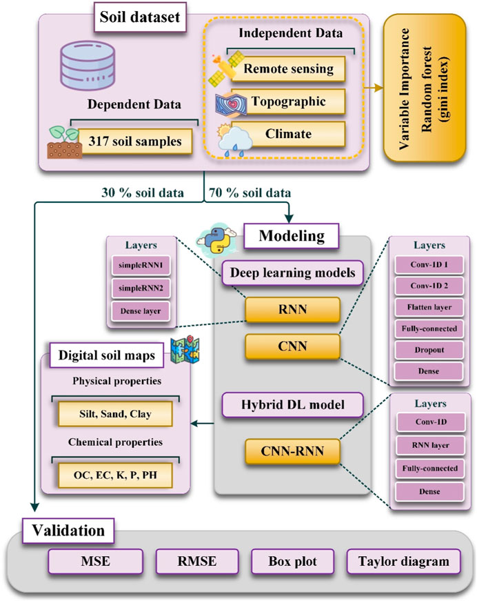
FIGURE 1. Research flowchart.
3 Materials and methods
3.1 Study area
The study area in Golestan province, one of Iran’s coastal provinces, occupies approximately 2,123 km2. Figure 2 shows the location of the study area and the distribution of soil samples. This area is located between 36° 56′ to 37° 35′ latitude and 54° 58′ to 55° 42′ longitude. The highest and lowest altitudes in this area are 0 and 1722 m above sea level, respectively. According to the National Meteorological Organization, the 8-year average (2014–2021) of meteorological records indicates an average annual rainfall of 456 mm in the study area. In addition, the average annual air temperature of the region is 19°C. As reported by the Soil and Water Research Institute of Iran, a large portion of the study area is dedicated to water wheat cultivation on the alluvial and valley plain. Also, the southern and northeastern sides of the study area are rugged terrain.
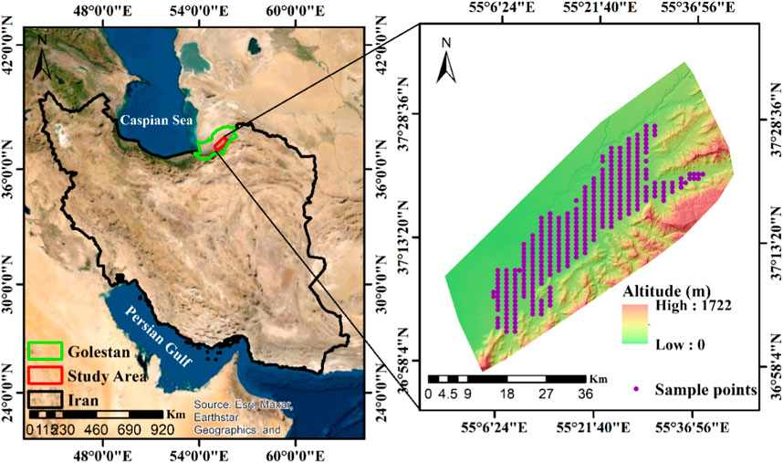
FIGURE 2. Case study with soil samples.
3.2 Soil sampling
The Soil and Water Research Institute collected 317 surface (0–30 cm) samples. An analysis has been conducted of eight soil properties, including chemical properties such as OC, EC, K, phosphorus P, pH, and physical properties such as the percentage of sand, silt, and clay. A handheld GPS device was used to record the coordinates at each sampling point, and the sampling resolution was 1 × 1 km. Five samples were taken from 0 to 30 cm depth, one at the main point and four at a 10 m distance from the main point, mixed and considered representative of that point. Each soil property has been analyzed differently. Disturbed soil samples were used to determine OC by the Walkley-Black oxidation method, K by the ammonium acetate extraction method (Richards, 1954), P by a Colorimeter (Olsen, 1954), pH and EC using a conductivity meter, and physical properties by the hydrometer method. These soil samples were used as dependent data. A statistical analysis of soil properties is shown in Table 1.
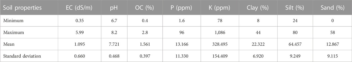
TABLE 1. Summary statistics of measured soil properties.
3.3 Environmental parameters
Three environmental categories were utilized, based on previous studies (Shahriari et al., 2019; Fathololoumi et al., 2020; Taghizadeh-Mehrjardi et al., 2022), expert insights, and the particular circumstances of the study area. There are three categories of effective variables for spatial prediction of soil properties: RS parameters [Band 1 (B1) to Band 7 (B7) of Landsat 8, brightness index (BI), coloration index (CI), clay index (CLI), enhanced vegetation index (EVI), hue index (HI), mid-Infrared (MIR), modified soil adjusted vegetation index (MSAVI), moisture stress index (MSI), normalized difference index (NDI), normalized difference vegetation index (NDVI), ratio vegetation index (RVI), redness index (RI), saturation index (SI), soil adjusted vegetation index (SAVI), triangular vegetation index (TVI), vegetation index (VI)], topographic parameters [aspect, elevation, slope, duration radiation (DR), general curvature, longitudinal curvature, modified catchment area (MCA), multi-resolution index of valley bottom flatness (MRVBF), multi-resolution ridgetop flatness index (MRRTF), plan curvature, profile curvature, stream power index (SPI), terrain ruggedness index (TRI), topographic wetness index (TWI), valley depth (VD), vector terrain ruggedness (VTR), vertical distance to channel network (VDCN)], and climatic parameters [air temperature, rainfall, soil temperature, land surface temperature (LST)]. Data were processed on ArcGIS 10.8, SAGA 8.2.1 software, and Google Earth Engine (GEE) (earthengine.google.com) platform. All data were projected to the WGS 84 zone 40 and resampled to a 30 × 30 m spatial resolution.
3.3.1 Remote sensing (RS) parameters
The RS images utilized were collected between January 1 and 30 December 2020. RS parameters (Figure 3) were calculated using the Google Earth Engine system (code.earthengine.google.com). To ensure data quality, the collection of Landsat 8 images was filtered to include only those with a cloud cover of less than 5%. Subsequently, the mean function was applied to each band of the Landsat 8 image collection, allowing for the calculation of average pixel values across the images. Atmospheric and radiometric correction of Landsat 8 imagery was conducted using the FLAASH (Fast line-of-sight atmospheric analysis of hypercubes) algorithm. There are 23 RS parameters listed in Table 2 with references.
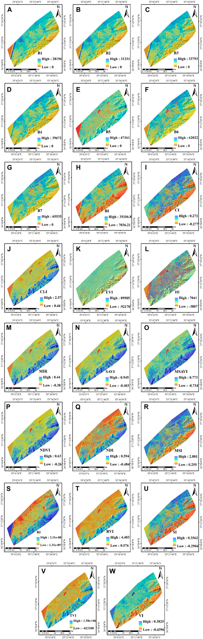
FIGURE 3. (Continued).
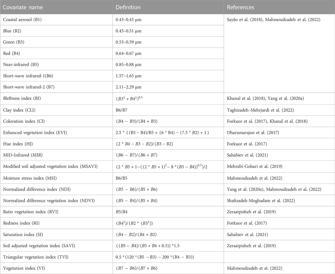
TABLE 2. Remote sensing parameters.
3.3.2 Topographic parameters
The digital elevation model (DEM) of the study area, which was derived from shuttle radar topography mission (SRTM) images in the GEE platform, was used to generate topographical parameters (with a 30 × 30 m spatial resolution). These parameters were processed using ArcGIS 10.8 and SAGA 8.2.1 software. Table 3 shows the topographical parameters. In Figure 4, 17 topographic parameters are shown.
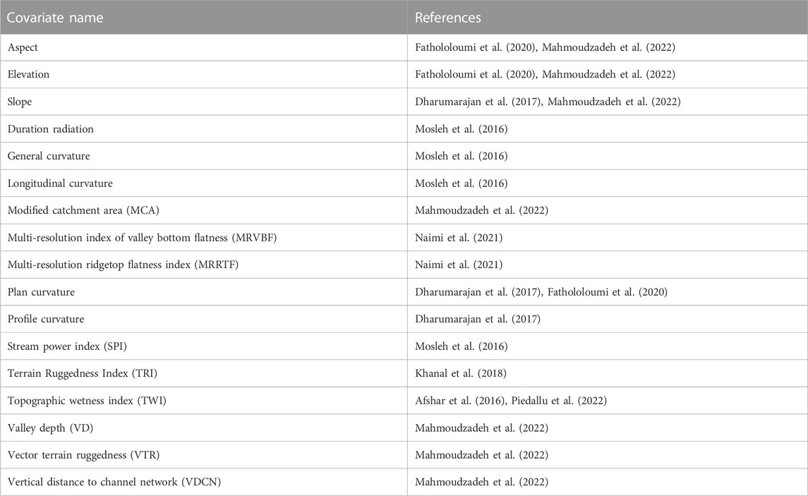
TABLE 3. Topographic parameters.
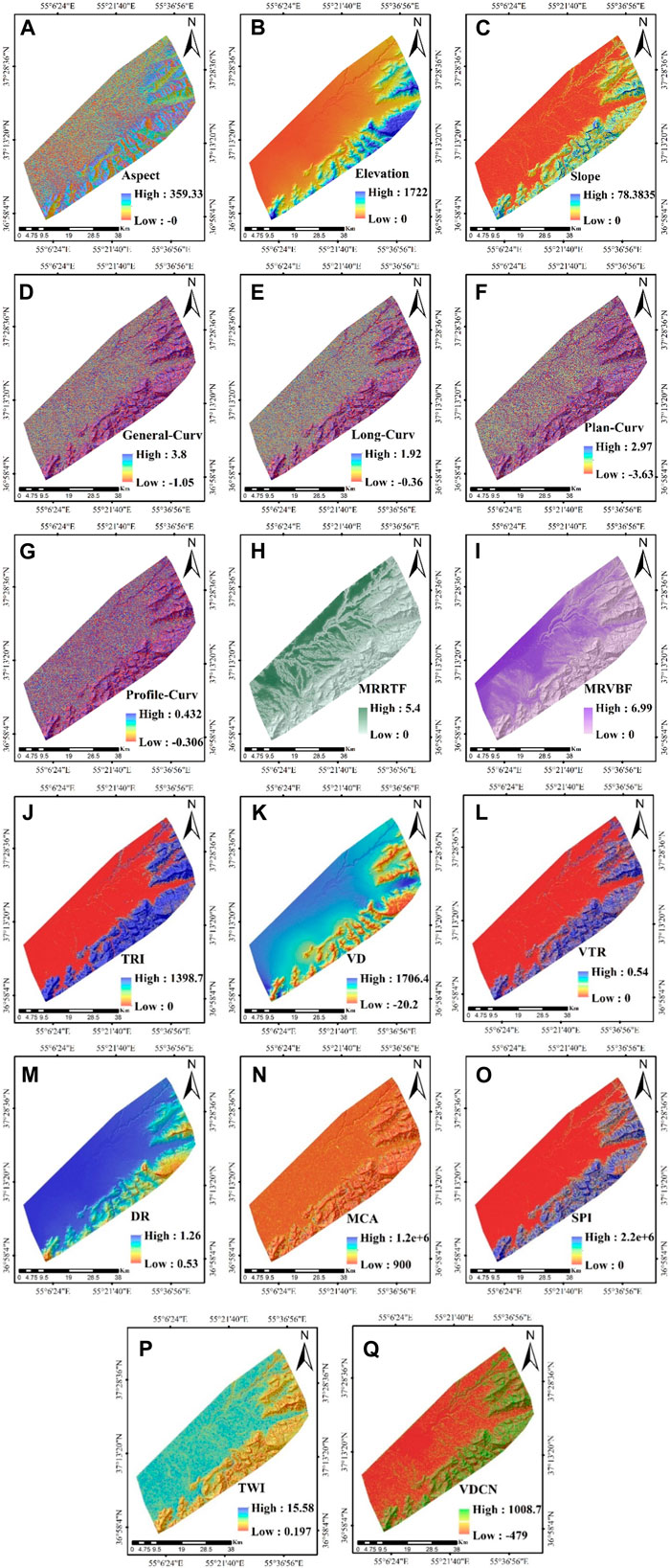
FIGURE 4. (Continued).
3.3.3 Climatic parameters
In this study, climatic data (Table 4) were calculated from the annual average (2014–2020) of 10 stations in the Golestan province (Figure 5). Iran Meteorological Organization provided these data. ArcGIS 10.8 software was used to prepare raster maps of climatic parameters using local polynomial, ordinary kriging, and global polynomial interpolation methods. The interpolation method with the least error was used. RMSE and RMSE% (Eq. 1 and Eq. 2) were computed to assess the interpolation methods' errors. In general, the lower the RMSE, the higher the interpolation accuracy. Acceptable value ranges for the RMSE% are less than 40% (Shogrkhodaei et al., 2021).
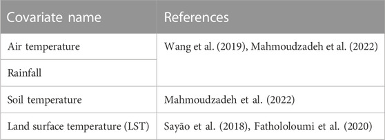
TABLE 4. Climatic parameters.
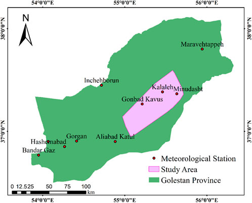
FIGURE 5. Meteorological stations in study area.
Where
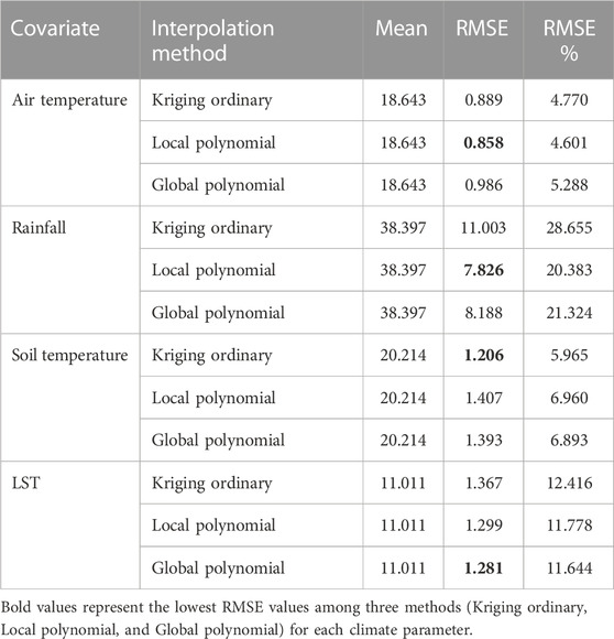
TABLE 5. Interpolation errors of climate parameters.
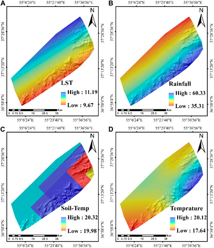
FIGURE 6. Climatic parameters: (A) LST, (B) rainfall, (C) soil temperature, and (D) temperature.
3.4 Training and testing dataset
The physical and chemical properties of the soil were considered dependent data, while environmental parameters were considered independent data. The dataset was divided into two subsamples, with 70% and 30% for training and testing, respectively. Table 6 contains the criteria that were considered effective parameters for each soil property based on the circumstances of the study area, the opinions of experts, and a review of previous studies (Kalambukattu et al., 2018; Fathololoumi et al., 2020; Sahabiev et al., 2021; Mahmoudzadeh et al., 2022).
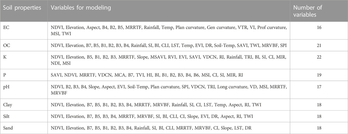
TABLE 6. Effective parameters for each soil property.
3.5 Prediction models
3.5.1 Convolutional neural network (CNN)
A CNN is a method of supervised DL that extracts and classifies features from high-dimensional data (Ma et al., 2021). A CNN is a multilayer perceptron that consists of one or more convolutional, max pooling, and fully connected layers. The input layer is an m × n matrix where m represents the number of soil samples, and n is the number of effective parameters for each soil property. Every element has a feature value. In the case where
Where * denotes the convolutional operator (Fang et al., 2021) and f is the rectified linear activation function (ReLU). The ReLU function is used here since it provides high performance in CNNs, compared to Sigmoid and Softmax (Scardapane et al., 2019; Azizi et al., 2020). Backpropagation algorithms optimize the parameters of each convolutional unit in each convolutional layer (Wang et al., 2019). Afterward, the obtained features are reorganized by fully connected layers (Fang et al., 2021). Finally, regression results are obtained from the output layer. Overfitting occurred after the CNN model was fitted to the data. Overfitting was solved by regularization in the two convolutional layers and dropout after the fully connected layer (Ng et al., 2020). An overview of the CNN algorithm is shown in Figure 7.
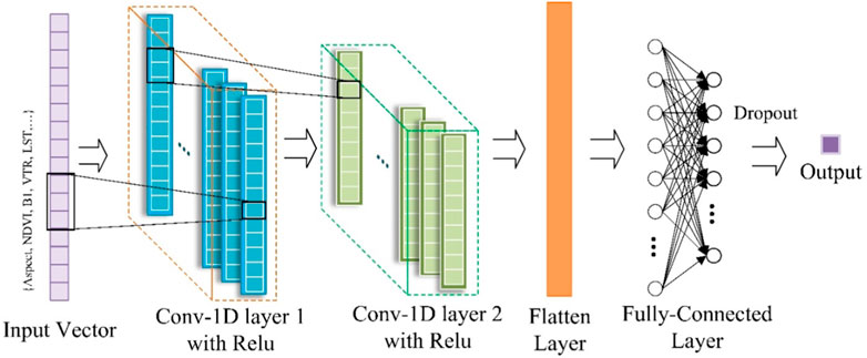
FIGURE 7. Architecture of the CNN algorithm.
3.5.2 Recurrent neural network (RNN)
RNNs are generally used for supervised learning, although they can also analyze sequential data (Ma et al., 2021). A deep RNN consists of several layers of RNNs stacked on top of one another. An RNN is a parameter updating function that outputs a new state (
Where
Where
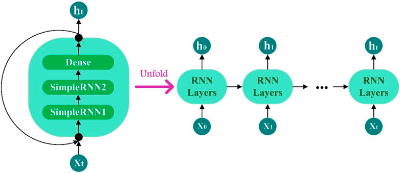
FIGURE 8. Architecture of the RNN algorithm.
3.5.3 Novel hybrid algorithm (CNN-RNN)
In this study, CNN and RNN algorithms were hybridized to overcome the disadvantages associated with each algorithm. CNNs have several limitations, including losing valuable information in the pooling layer and ignoring the correlation between the part and the whole of input data. In addition, RNNs have the problem of exploding and vanishing gradients (Shen et al., 2022). This research proposed a state-of-the-art hybridization of CNNs and RNNs owing to the limitations mentioned. DL hybrid CNN-RNN model illustrates the ability of CNNs to extract features and RNNs to learn temporal dependencies (Barzegar et al., 2021; Nasir et al., 2021). The architecture of the CNN-RNN model is shown in Figure 9. In Figure 9, raw data is normalized and pre-processed before being fed into the convolution layer, where the model extracts spatial features. The output of the convolution layer is passed to the RNN layer to learn temporal dependencies. To organize the features obtained from the RNN layer, this layer transmits the predicted values to the fully connected layer. Lastly, the fully connected layer with one neuron provides the predicted value of the soil property.
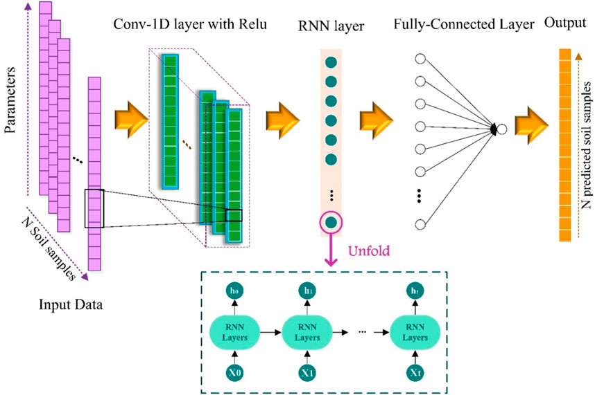
FIGURE 9. Architecture of the novel hybrid algorithm.
3.5.4 Variable importance using random forest (RF)
An RF algorithm is used to determine the importance of environmental parameters for each soil property based on the Gini index. RF is a tree algorithm for classification and regression problems that can considerably reduce computation time (Nam and Wang, 2020; Farhangi et al., 2022). The Gini index is a number describing the quality of the split of a node on a variable. The Gini index is calculated for the variable
After separating into two sub-nodes and selecting optimal features, the Gini index at the parent node decreases to its maximum value. Therefore, it is possible to determine the average reduction in the Gini index for each variable
Where
3.6 Model performance
Two evaluation metrics were used to assess the efficiency of the models, namely, RMSE and MSE, as shown in Eqs 1, 10, respectively. MSE and RMSE evaluate a model’s ability to predict data. The lower values of MSE and RMSE indicate higher modeling accuracy (Razavi-Termeh et al., 2021).
In Eq. 10,
4 Results
4.1 Correlation analysis
The research employed the Pearson correlation coefficient to elucidate the intricate relationships between soil properties and environmental parameters, as depicted in Figure 10. These analyses unveiled a diverse landscape of associations, with varying strengths and directions. For instance, concerning EC, a notable positive relationship with MMRTF (0.12) was discerned, while EC exhibited notably negative associations with elevation (−0.26) and temperature (−0.26). These findings underscore the intricate interplay between EC and these environmental parameters. For PH, relatively mild negative associations with NDVI (−0.091) and modest positive connections with B2 (0.096) were observed. OC exhibited substantial positive relationship with DR (0.24), coupled with relatively robust negative associations with temperature (−0.26) and LST (−0.28). P displayed relatively solid positive correlations with VDCN (0.12) and negative relationships with B7 (−0.099). For K, there were strong negative associations with rainfall (−0.33) and elevation (−0.33) and a relatively robust positive connection with B1 (0.11). In the context of Silt, a relatively strong positive relationship with CI (0.27) was evident, while relatively strong negative relationships were observed with NDVI (−0.25) and CLI (−0.24). Sand showed a relatively robust positive association with DR (0.11) and a negative relationship with LST (−0.19). Lastly, Clay exhibited a relatively strong positive connection with MRVBF (0.18) and a relatively robust negative relationship with B7 (−0.26).
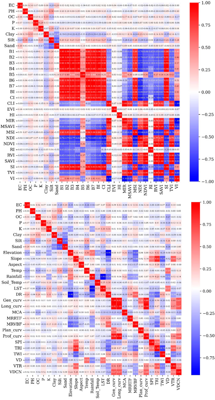
FIGURE 10. The correlation coefficients between environmental parameters and soil properties.
4.2 Variable importance
After identifying the parameters that affect the chemical and physical properties of the soil, the RF algorithm was used to assess variable importance. The relative importance of each variable is shown in Figure 11 for the various soil properties. The results show that MRRTF (0.14), air temperature (0.12), and rainfall (0.11) were the most influential parameters for EC prediction (Figure 11A). As shown in Figure 11B, the most significant parameters for the prediction of OC were air temperature (0.22), LST (0.13), and rainfall (0.08). The most effective parameters for K prediction were elevation (0.19), rainfall (0.18), and MIR (0.08), respectively (Figure 11C). According to Figure 11D, CI (0.23), VDCN (0.14), and MCA (0.06) were the most influential parameters for P prediction.
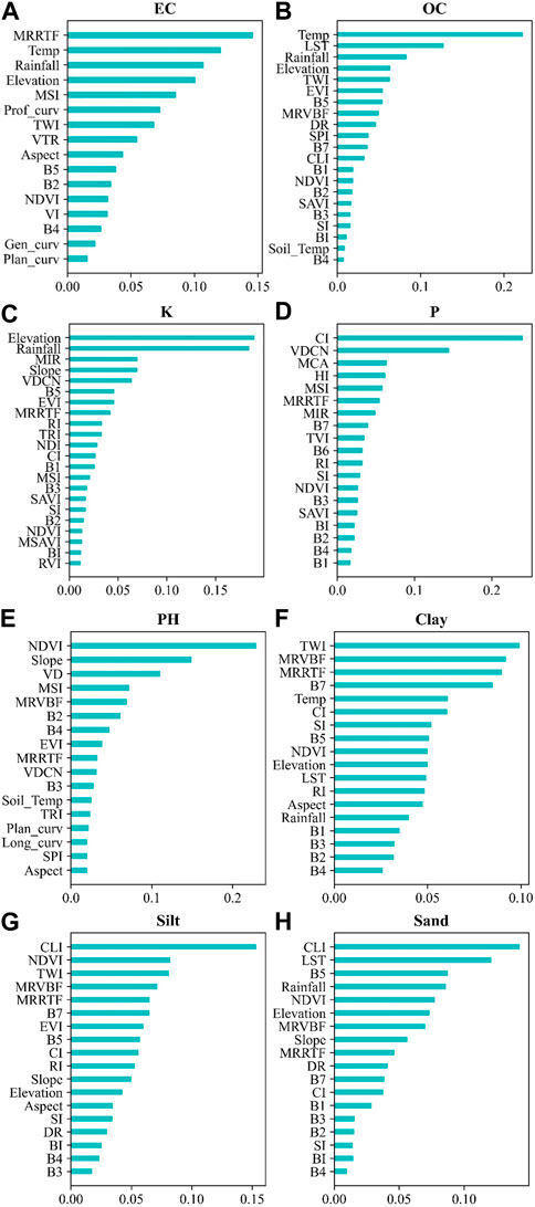
FIGURE 11. Importance of environmental parameters for soil properties: (A) EC, (B) OC, (C) K, and (D) P, (E) pH, (F) Clay, (G) Silt, and (H) Sand.
NDVI (0.23), Slope (0.15), and VD (0.11) had the most significant impact on soil pH (Figure 11E). TWI (0.1), MRVBF (0.0925), and MRRTF (0.09) were the most effective parameters for clay content (Figure 11F). CLI (0.15), NDVI (0.08), and TWI (0.08) were the most influential parameters for silt prediction (Figure 11G). The most influential parameters for predicting sand content were CLI (0.14), LST (0.12), and B5 (0.09) (Figure 11H).
In general, based on the results obtained among the climatic parameters of rainfall, air temperature, and LST, among the RS parameters of NDVI, CI, and MIR, and among the topographic parameters of elevation, MRRTF, slope, VDCN, MCA, and VD had the highest effect on the chemical properties of the soil. Physical properties were also affected by climatic factors such as rainfall, and LST, RS parameters such as NDVI, B5, CLI, and B7, and topographic parameters such as TWI, MRVBF, and MRRTF.
4.3 Model development
Using DL algorithms, spatial modeling and prediction of soil properties were performed on a computer with an Intel Cori7 CPU @2.80 GHz and 16 GB of RAM. Each model is developed in the Google Colab environment (https://colab.research.google.com) using the Python programming language and DL libraries such as Keras and TensorFlow. Furthermore, the Numpy, CSV, Scikit-Learn, and Matplotlib libraries were used to analyze data, evaluate models, and plot results. Before modeling, data must be preprocessed and normalized. Parameter tuning was performed using grid search. 5-fold cross-validation has been used to prevent over- or under-fitting of the model, estimate its performance in new data and remove any bias in the data (Tavakkoli Piralilou et al., 2022). Despite the advantages of DL models, some practical limitations exist, such as the difficulty of determining optimal hyperparameters for specific problems and data sets. Model performance is directly impacted by choice of optimal parameters (Drumond et al., 2019). Therefore, GridSearch is used to determine the number of filters in each convolution layer, its kernel size, the number of nodes in the fully connected layers (except for the output layer with one node), the number of nodes in the SimpleRNN layer, the activation functions, and the optimizer functions (Table 7).
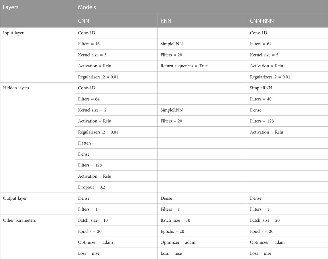
TABLE 7. A description of the layers and parameters used in DL models.
The percentages of training and testing data for soil samples are 70% and 30%, respectively. Input matrices for each model consisting of m rows and n columns, where m indicates the number of soil samples and n indicates the number of effective parameters for each soil property. As shown in Table 6, the parameters affecting OC, EC, K, P, pH, Silt, Sand, and Clay was 21, 16, 22, 19, 17, 18, 18, and 18, respectively. CNN, RNN, and CNN-RNN models were used for modeling.
MSE (Eq. 10) is employed as the loss function in the developed models. It is widely used as a loss function estimating the parameters of nonlinear models such as supervised neural networks (Sangari and Sethares, 2015). Loss function plots are shown in Figure 12. It is clear from comparing the plots of all three models that the hybrid model is more accurate in all the physical and chemical properties of soil than the other models.
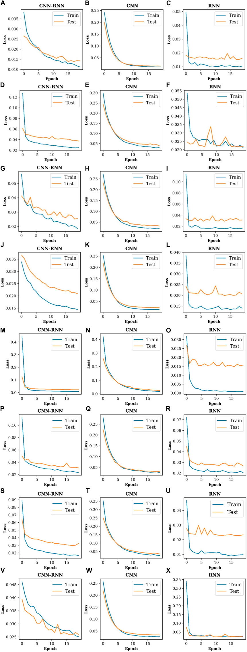
FIGURE 12. (Continued).
4.4 Comparison of prediction models
Using train and test data, CNN, RNN, and CNN-RNN models were evaluated using MSE and RMSE. Table 8 demonstrates the outcomes of various metrics in the training and testing phases. CNN model calculated MSE (0.020264%2, 0.020984%2) and RMSE (0.142351%, 0.144859%) in the training and testing phases of OC prediction, respectively. Furthermore, RNN produced MSE (0.018823%2, 0.02395%2) and RMSE (0.137196%, 0.154757%) for OC, whereas CNN-RNN obtained MSE (0.018533%2, 0.020718%2) and RMSE (0.136137%, 0.143939%) in the training and testing phases, respectively. CNN model calculated MSE (0.010068 dS2/m2, 0.011895 dS2/m2) and RMSE (0.10034 dS/m, 0.109062 dS/m) for EC during the training and testing phases, respectively. Moreover, MSE (0.009476 dS2/m2, 0.013556 dS2/m2) and RMSE (0.097346 dS/m, 0.11643 dS/m) were generated by the RNN model for EC, while the hybrid CNN-RNN model produced MSE (0.009187 dS2/m2, 0.011353 dS2/m2) and RMSE (0.095848 dS/m, 0.106551 dS/m) in the training and testing phases, respectively. MSE (0.015725 ppm2, 0.02192 ppm2) and RMSE (0.1254 ppm, 0.148054 ppm) were computed by the CNN model for K during the training and testing phases, respectively. In addition, RNN calculated MSE (0.015264 ppm2, 0.020387 ppm2) and RMSE (0.123549 ppm, 0.142782 ppm) for K, whereas CNN-RNN obtained MSE (0.014051 ppm2, 0.019809 ppm2) and RMSE (0.118535 ppm, 0.140743 ppm) in the training and testing phases, respectively.
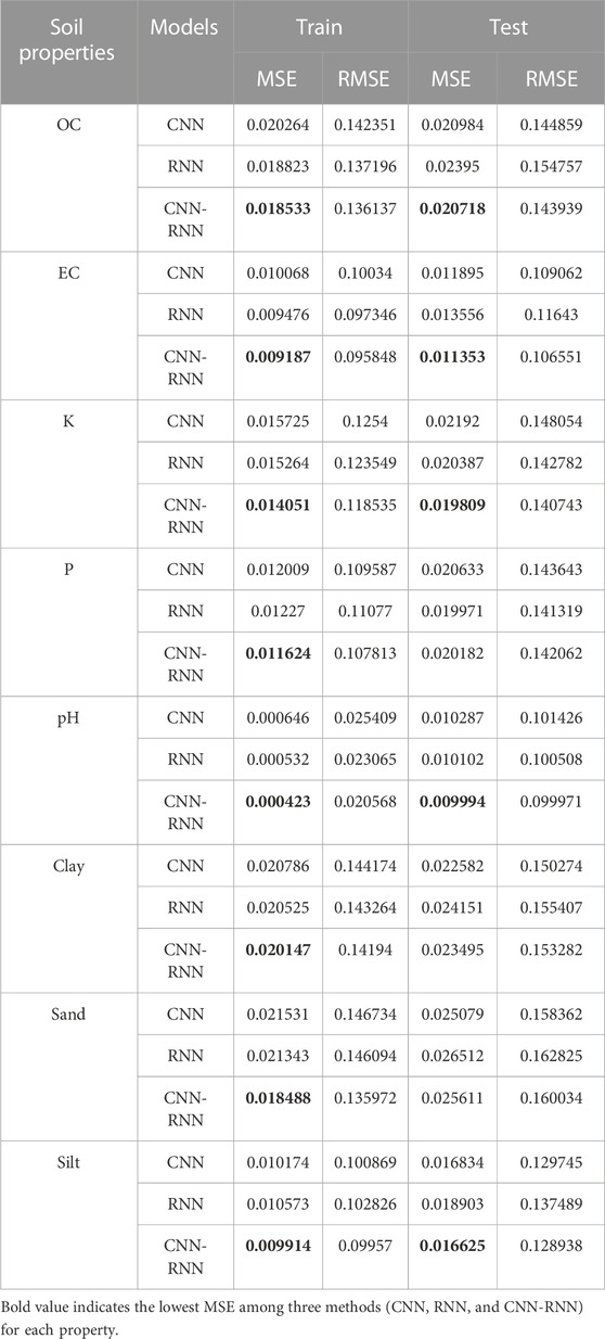
TABLE 8. Results of prediction models in training and testing phases.
As a result of the CNN model, MSE (0.012009 ppm2, 0.020633 ppm2) and RMSE (0.109587 ppm, 0.143643 ppm) are calculated during the training and testing phases of P prediction, respectively. Furthermore, RNN produced MSE (0.018823 ppm2, 0.02395 ppm2) and RMSE (0.137196 ppm, 0.154757 ppm) for P, while CNN-RNN generated MSE (0.018533 ppm2, 0.020718 ppm2) and RMSE (0.136137 ppm, 0.143939 ppm) in the training and testing phases, respectively. CNN model calculated MSE (0.000646, 0.010287) and RMSE (0.025409, 0.101426) for soil pH during the training and testing phases, respectively. Moreover, MSE (0.000532, 0.010102) and RMSE (0.023065, 0.100508) were generated by the RNN model for soil pH, while the hybrid CNN-RNN model produced MSE (0. 000423, 0. 009994) and RMSE (0. 020568, 0. 099971) in the training and testing phases, respectively. MSE (0.020786%2, 0.022582%2) and RMSE (0.144174%, 0.150274%) were computed by the CNN model for clay during the training and testing phases, respectively. In addition, RNN obtained MSE (0.020525%2, 0.024151%2) and RMSE (0.143264%, 0.155407%) for clay, whereas CNN-RNN calculated MSE (0.020147%2, 0.023495%2) and RMSE (0.14194%, 0.153282%) in the training and testing phases, respectively. CNN model calculated MSE (0.021531%2, 0.025079%2) and RMSE (0.146734%, 0.158362%) in the training and testing phases of sand prediction, respectively. Furthermore, RNN produced MSE (0.021343%2, 0.026512%2) and RMSE (0.146094%, 0.162825%) for sand, whereas CNN-RNN obtained MSE (0.018488%2, 0.025611%2) and RMSE (0.135972%, 0.160034%) in the training and testing phases, respectively. As a result of the CNN model, MSE (0.010174%2, 0.016834%2) and RMSE (0.100869%, 0.129745%) are calculated during the training and testing phases of silt prediction, respectively. Furthermore, RNN produced MSE (0.010573%2, 0.018903%2) and RMSE (0.102826%, 0.137489%) for silt, while CNN-RNN generated MSE (0.009914%2, 0.016625%2) and RMSE (0.09957%, 0.128938%) in the training and testing phases, respectively.
Generally, for all properties in the training phase, the hybrid CNN-RNN model had the highest performance based on MSE and RMSE. According to the testing phase, the best model for most properties was the hybrid CNN-RNN model, while the most appropriate model for P, clay, and sand properties was the RNN, CNN, and CNN models, respectively.
Figure 13 graphically compares the performance of the three developed models, RNN, CNN, and CNN-RNN, with the soil samples dataset using box plots. The minimum and maximum values of each property are shown at the ends of purple dashed whiskers outside the box, and the median is indicated by a notch within each box. Outliers are plotted in circles outside the box. This figure showed that for most soil properties, the hybrid CNN-RNN model achieved higher prediction accuracy with its shape identical to the actual values than other models.
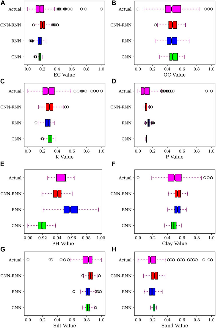
FIGURE 13. Box plots for comparison of the hybrid CNN-RNN model, RNN and CNN models for soil properties: (A) EC, (B) OC, (C) K, and (D) P, (E) pH, (F) Clay, (G) Silt, and (H) Sand.
Figure 14 illustrates Taylor diagrams, where the purple point indicates the reference point, and red lines show the distance from the reference point. The CNN-RNN model has a higher correlation and a lower error value for all soil properties except soil pH (Figure 14E) compared to the CNN, and RNN models.
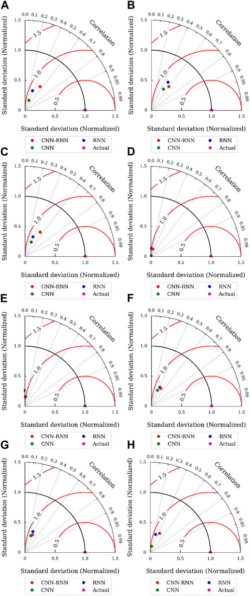
FIGURE 14. Taylor diagram for comparison of model performance: (A) EC, (B) OC, (C) K, (D) P, (E) pH, (F) Clay, (G) Silt, (H) Sand.
4.5 Spatial predication of soil properties
After model development, the modeling results were generalized to the entire study area for each soil property. The spatial predictions of the target soil properties at 30 × 30 m spatial resolution are illustrated in Figure 15. As shown on the prediction map of the CNN model (Figure 15C), EC properties decreases with increasing elevation. There is a similar pattern in the prediction maps of RNN, and CNN-RNN models, where the amount of soil EC is scattered, and in the north and northeast, the amount is less than in the southeast. However, the range of EC changes in the RNN prediction map is greater than that in the hybrid model. Regarding OC prediction maps, the RNN and CNN-RNN model show a similar pattern. OC prediction maps for RNN and CNN-RNN models indicate that the value of OC increases from north to south. Higher-altitude areas have more OC, while low-altitude and the plain regions have less OC. The OC map in the CNN model is nearly identical to the maps in the other models, except that the OC value in the eastern region is substantially lower. The K prediction maps in both RNN and CNN models are similar. However, the RNN model exhibits a greater range of K changes than the CNN model. Both of these maps indicate that K concentrations increase as altitude decreases. However, CNN-RNN has predicted different amounts of K for high-altitude areas, where some areas have average K levels and others have lower levels. There is a similar pattern in the P prediction maps of RNN and CNN-RNN models. However, the P change range of the hybrid model is smaller than that of the RNN model (Figure 15K). As illustrated in Figures 15J–L, P levels decrease with increasing altitude. According to the CNN model, P levels in the east and northeast of the region are average compared to the other two models. Furthermore, the hybrid model exhibits a more extensive range of P changes than the CNN model. Based on the CNN model, pH distribution on the soil surface is not directly related to altitude. In contrast, the prediction map of the RNN model indicates higher pH in high-altitude areas than in other areas, while in the CNN-RNN model, soil pH decreases as altitude increases. In terms of clay prediction maps, the CNN and CNN-RNN models show a similar pattern. At high altitudes, there was a concentration of medium clay content, while in the northeast, there was low clay content. However, in the RNN prediction map, the clay content is low in high-altitude areas. However, the greatest concentration of clay was found in the west, as shown by all three maps. The Sand prediction map in both RNN and CNN-RNN models is similar. The lowest amount of Sand can be observed in the high-altitude areas, while the highest amount of Sand can be found in the central and northern parts of the region. The RNN model provides a wider range of sand changes than the hybrid model. The CNN model’s prediction map is similar to the other models' map; however, it shows more sand in the western and southwestern regions. The spatial distribution of silt in CNN and CNN-RNN maps is similar. Based on these two maps, high-altitude areas have more silt content than low-altitude areas. Furthermore, the CNN-RNN model displays a more extensive range of silt changes than the CNN model. In contrast, silt content at high-altitudes is average on the CNN model map.
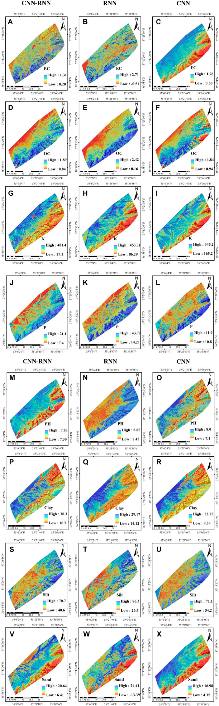
FIGURE 15. (Continued).
5 Discussion
5.1 Variable importance analysis
Variable importance was calculated for each soil property using an RF algorithm based on the Gini index. MRRTF and air temperature were the most important criteria for EC property. In agreement with these results, Dharumarajan et al. (2017) and Taghizadeh-Mehrjardi et al. (2022) reported that MRRTF and air temperature are influential auxiliary variables for EC modeling. There is evidence that temperature can increase fluid viscosity, affecting EC, and soil EC can also increase as temperature increases (Bai et al., 2013). The most influential variable for OC prediction was air temperature. Similar results were reported by Taghizadeh-Mehrjardi et al. (2022). Temperature and rainfall can impact OC and nitrogen dynamics by affecting net primary productivity, biological activity, litter accumulation and decomposition rates (Zhou et al., 2021). Another parameter affecting OC was LST, which is directly related to OC (Sayão et al., 2018). The most significant variables in predicting K property were elevation and rainfall. Elevation affects the chemical and physical properties of soil owing to its effects on rainfall, temperature, and vegetation. The K content of the soil decreases as elevation increases (Badía et al., 2016). The results of the K property were consistent with the results of Mahmoudzadeh et al. (2022). Precipitation has an indirect effect on soil pH (Yang et al., 2020b). In terms of P property prediction, CI was the most influential parameter. Most multispectral and hyperspectral sensors can determine soil CI, which is one of the most useful parameters for describing and identifying soil. Organic matter is usually found in greater quantities in dark soils than in light soils (Novák et al., 2018; Sahabiev et al., 2021). In soil pH prediction, NDVI was the most important parameter. Previous studies have shown that NDVI is one of the most critical parameters in the spatial prediction of soil pH (Mazur et al., 2022; Taghizadeh-Mehrjardi et al., 2022). Environmental parameters such as temperature, rainfall, nitrogen, and soil pH influence NDVI. A higher NDVI corresponds to a lower soil pH (Piedallu et al., 2019). Higher NDVI values in a decrease in pH owing to higher concentrations of H+ ions in the soil as a result of organic matter decomposition (Banday et al., 2019). The most influential parameter for spatial prediction of clay was TWI. The results of this research are consistent with the results of Afshar et al. (2016) and Mehrabi-Gohari et al. (2019). TWI shows the influence of topography on the location and amount of moisture accumulation in soil or groundwater (Mehrabi-Gohari et al., 2019). Humidity and high temperatures lead to chemical weathering and clay mineral production (Liu et al., 2020). The most influential parameter for spatial prediction of sand and silt was CLI. Taghizadeh-Mehrjardi et al. (2022) observed similar results to the current study. By examining Pearson’s correlation coefficient, Shahriari et al. (2019) found a positive and negative correlation between CLI and Silt content and Sand content, respectively.
Overall, climatic parameters such as air temperature and rainfall had the greatest influence on chemical properties compared to other environmental parameters. Topographic parameters such as elevation, MRRTF, slope, and VDCN had a greater impact on soil chemical properties than CI and NDVI parameters. Topographic (TWI, MRVBF, and MRRTF), RS (CLI, NDVI), and climatic (LST) parameters were effective at predicting soil physical properties.
5.2 Comparison and analysis of models
Based on the results of the evaluation metrics, CNN-RNN model had the highest accuracy, followed by RNN and CNN models. Hybridization of convolutional and recurrent networks can provide powerful tools for predicting the spatial distribution of variables (Faraji et al., 2022). In the proposed hybrid model, convolution layers extract the spatial features, while RNN layers are used to model the temporal dependencies. In recent years, the hybridization of CNN and RNN performed better than other algorithms and regression models. Tovar et al. (2020) found that the hybrid CNN-RNN model was more accurate at predicting photovoltaic power than the RNN model and the Lasso and Ridge regression models. In another study conducted by X. Zhang et al. (2019), the CNN-RNN model proved to be more accurate and superior to CNN, multilayer perceptron, and support vector regression (SVR) models in predicting the remaining useful life. Furthermore, Barzegar et al. (2021) found that the CNN-RNN model performed better than the independent SVR, and RF models in water level forecasting.
A deep neural network focuses on a single task, limiting its ability to execute other tasks (Nasir et al., 2021). It is well known that CNN can recognize spatial features from datasets (Yusuf et al., 2021). CNNs have the drawback of overfitting the input data, which results in inadequate performance on new datasets (Barzegar et al., 2021). Meanwhile, RNNs are applied to analyze temporal dependencies (Jenifer et al., 2022). Gradient loss is a common problem in RNNs (with gradient-based and back-propagation learning methods). Gradient vanishing occurs when training long data sequences. As a result, the gradient of the loss function approaches 0, making training the network challenges (Tovar et al., 2020). In this regard, the inability of neural networks to solve problems simultaneously becomes the advantage of hybrid methods (Nasir et al., 2021).
As compared to CNN, the RNN model performed better. RNN networks are distinguished from other DL algorithms by their ability to process temporal information and use sequential data. As embedded structures in data sequences contain valuable information, this property is essential for various applications (Alzubaidi et al., 2021). In the classification of sentence-level relationships, a basic RNN structure can outperform a CNN (Zhang and Wang, 2016).
5.3 Research strengths and weaknesses
One of the strengths of this study is the use of a state-of-the-art hybrid CNN-RNN model for spatial prediction of soil properties. Through the use of this method, it has become more accurate to predict the chemical and physical properties of soils. This research used all the physical and chemical properties of soil. In the current study, hybrid modeling was found to be successful in improving the predictive accuracy of all soil properties. The use of optical images for obtaining vegetation indices and other RS parameters, which are more suitable than other satellite images, is another strength of this research. The lack of a feature selection approach and the lack of optimization of the hyperparameters of the DL algorithms utilizing metaheuristic algorithms are the research’s shortcomings.
6 Conclusion
In this study, CNN, RNN, and a hybrid CNN-RNN algorithm were used to predict the physical and chemical properties of soil. Optical satellite images were used for soil property estimations due to their advantages, such as the ease of extracting vegetation indices, soil moisture and soil conditions, and other RS parameters. Research findings can be summarized as follows: 1) Based on the RF algorithm, MRRTF, air temperature, elevation, CI, NDVI, CLI, TWI, and CLI had a significant effect on EC, OC, K, P, pH, sand, clay, and Silt, respectively. 2) The results showed that TWI and CLI were the most influential parameters among the physical properties, while temperature and rainfall were the most influential parameters among the chemical properties. 3) Based on the evaluation metrics, the hybrid CNN-RNN model was more accurate at predicting soil chemical and physical properties than both RNN and CNN models. 4) Sand property had the highest accuracy in prediction among physical properties, while OC had the highest accuracy in chemical properties.
Soil properties can be mapped at the regional level using the implemented hybrid model. These maps can be applied to various applications, such as precision agriculture, soil protection, crop planning based on the soil’s nutrient potential, and irrigation management based on the soil’s physical properties. The following recommendations are made for future research: 1) Using a metaheuristic algorithm, principal component analysis, and other feature selection methods to reduce the number of independent parameters and improve prediction accuracy. 2) A hybridization of other DL model, such as LSTM and CNN, can be applied to develop a novel model for soil spatial prediction.
Data availability statement
The raw data supporting the conclusion of this article will be made available by the authors, without undue reservation.
Author contributions
FH: Conceptualization, Data curation, Formal Analysis, Methodology, Software, Validation, Visualization, Writing–original draft. SR-T: Conceptualization, Investigation, Validation, Writing–review and editing. AS-N: Funding acquisition, Project administration, Resources, Supervision, Writing–review and editing. S-MC: Funding acquisition, Project administration, Supervision, Writing–review and editing. MJ: Data curation, Validation, Writing–review and editing.
Funding
The author(s) declare financial support was received for the research, authorship, and/or publication of this article. This work was supported in part by the ITRC Support Program under Grant IITP-2023-RS-2022-00156354 and in part by the Metaverse Support Program to Nurture the Best Talents under Grant IITP-2023-RS-2023-00254529 funded by the Ministry of Science and ICT of Korea and the Institute of Information and Communications Technology Planning and Evaluation (IITP) and in part by the Ministry of Trade, Industry and Energy and Korea Institute for Advancement of Technology under Grant P0016038.
Conflict of interest
The authors declare that the research was conducted in the absence of any commercial or financial relationships that could be construed as a potential conflict of interest.
Publisher’s note
All claims expressed in this article are solely those of the authors and do not necessarily represent those of their affiliated organizations, or those of the publisher, the editors and the reviewers. Any product that may be evaluated in this article, or claim that may be made by its manufacturer, is not guaranteed or endorsed by the publisher.
References
Afshar, F. A., Ayoubi, S., Besalatpour, A. A., Khademi, H., and Castrignano, A. (2016). Integrating auxiliary data and geophysical techniques for the estimation of soil clay content using CHAID algorithm. J. Appl. Geophys. 126, 87–97. doi:10.1016/j.jappgeo.2016.01.015
Ahmed, A. M., Deo, R. C., Ghahramani, A., Feng, Q., Raj, N., Yin, Z., et al. (2022). New double decomposition deep learning methods for river water level forecasting. Sci. Total Environ. 831, 154722. doi:10.1016/j.scitotenv.2022.154722
Al-Dahidi, S., Ayadi, O., Adeeb, J., Alrbai, M., and Qawasmeh, B. R. (2018). Extreme learning machines for solar photovoltaic power predictions. Energies 11 (10), 2725. doi:10.3390/en11102725
Alygizakis, N., Giannakopoulos, T., Τhomaidis, N. S., and Slobodnik, J. (2022). Detecting the sources of chemicals in the Black Sea using non-target screening and deep learning convolutional neural networks. Sci. Total Environ. 847, 157554. doi:10.1016/j.scitotenv.2022.157554
Alzubaidi, L., Zhang, J., Humaidi, A. J., Al-Dujaili, A., Duan, Y., Al-Shamma, O., et al. (2021). Review of deep learning: concepts, CNN architectures, challenges, applications, future directions. J. big Data 8 (1), 53–74. doi:10.1186/s40537-021-00444-8
Amani, M., Salehi, B., Mahdavi, S., and Brisco, B. (2018). Spectral analysis of wetlands using multi-source optical satellite imagery. ISPRS J. Photogrammetry Remote Sens. 144, 119–136. doi:10.1016/j.isprsjprs.2018.07.005
Ayoubi, S., Mokhtari, J., Mosaddeghi, M. R., and Zeraatpisheh, M. (2018). Erodibility of calcareous soils as influenced by land use and intrinsic soil properties in a semiarid region of central Iran. Environ. Monit. Assess. 190, 192–212. doi:10.1007/s10661-018-6557-y
Azizi, A., Gilandeh, Y. A., Mesri-Gundoshmian, T., Saleh-Bigdeli, A. A., and Moghaddam, H. A. (2020). Classification of soil aggregates: a novel approach based on deep learning. Soil Tillage Res. 199, 104586. doi:10.1016/j.still.2020.104586
Badía, D., Ruiz, A., Girona, A., Martí, C., Casanova, J., Ibarra, P., et al. (2016). The influence of elevation on soil properties and forest litter in the Siliceous Moncayo Massif, SW Europe. J. Mt. Sci. 13 (12), 2155–2169. doi:10.1007/s11629-015-3773-6
Bai, W., Kong, L., and Guo, A. (2013). Effects of physical properties on electrical conductivity of compacted lateritic soil. J. Rock Mech. Geotechnical Eng. 5 (5), 406–411. doi:10.1016/j.jrmge.2013.07.003
Banday, M., Bhardwaj, D., and Pala, N. A. (2019). Influence of forest type, altitude and NDVI on soil properties in forests of North Western Himalaya, India. Acta Ecol. Sin. 39 (1), 50–55. doi:10.1016/j.chnaes.2018.06.001
Barzegar, R., Aalami, M. T., and Adamowski, J. (2021). Coupling a hybrid CNN-LSTM deep learning model with a boundary corrected maximal overlap discrete wavelet transform for multiscale lake water level forecasting. J. Hydrology 598, 126196. doi:10.1016/j.jhydrol.2021.126196
Bodaghabadi, M. B., Martínez-Casasnovas, J., Salehi, M. H., Mohammadi, J., Borujeni, I. E., Toomanian, N., et al. (2015). Digital soil mapping using artificial neural networks and terrain-related attributes. Pedosphere 25 (4), 580–591. doi:10.1016/s1002-0160(15)30038-2
Dharumarajan, S., Hegde, R., and Singh, S. (2017). Spatial prediction of major soil properties using Random Forest techniques-A case study in semi-arid tropics of South India. Geoderma Reg. 10, 154–162. doi:10.1016/j.geodrs.2017.07.005
Dhruv, P., and Naskar, S. (2020). Image classification using convolutional neural network (CNN) and recurrent neural network (RNN): a review. Mach. Learn. Inf. Process., 367–381. doi:10.1007/978-981-15-1884-3_34
Drumond, T. F., Viéville, T., and Alexandre, F. (2019). Bio-inspired analysis of deep learning on not-so-big data using data-prototypes. Front. Comput. Neurosci. 12, 100. doi:10.3389/fncom.2018.00100
Fang, Z., Wang, Y., Peng, L., and Hong, H. (2021). A comparative study of heterogeneous ensemble-learning techniques for landslide susceptibility mapping. Int. J. Geogr. Inf. Sci. 35 (2), 321–347. doi:10.1080/13658816.2020.1808897
Farahani, M., Razavi-Termeh, S. V., and Sadeghi-Niaraki, A. (2022). A spatially based machine learning algorithm for potential mapping of the hearing senses in an urban environment. Sustain. Cities Soc. 80, 103675. doi:10.1016/j.scs.2022.103675
Faraji, M., Nadi, S., Ghaffarpasand, O., Homayoni, S., and Downey, K. (2022). An integrated 3D CNN-GRU deep learning method for short-term prediction of PM2. 5 concentration in urban environment. Sci. Total Environ. 834, 155324. doi:10.1016/j.scitotenv.2022.155324
Farhangi, F., Sadeghi-Niaraki, A., Nahvi, A., and Razavi-Termeh, S. V. (2022). Spatial modelling of accidents risk caused by driver drowsiness with data mining algorithms. Geocarto Int. 37 (9), 2698–2716. doi:10.1080/10106049.2020.1831626
Fathololoumi, S., Vaezi, A. R., Alavipanah, S. K., Ghorbani, A., Saurette, D., and Biswas, A. (2020). Improved digital soil mapping with multitemporal remotely sensed satellite data fusion: a case study in Iran. Sci. Total Environ. 721, 137703. doi:10.1016/j.scitotenv.2020.137703
Forkuor, G., Hounkpatin, O. K., Welp, G., and Thiel, M. (2017). High resolution mapping of soil properties using remote sensing variables in south-western Burkina Faso: a comparison of machine learning and multiple linear regression models. PloS one 12 (1), e0170478. doi:10.1371/journal.pone.0170478
Garajeh, M. K., Malakyar, F., Weng, Q., Feizizadeh, B., Blaschke, T., and Lakes, T. (2021). An automated deep learning convolutional neural network algorithm applied for soil salinity distribution mapping in Lake Urmia, Iran. Sci. Total Environ. 778, 146253. doi:10.1016/j.scitotenv.2021.146253
Guo, J., Liu, Y., Yang, Q., Wang, Y., and Fang, S. (2021). GPS-based citywide traffic congestion forecasting using CNN-RNN and C3D hybrid model. Transp. A Transp. Sci. 17 (2), 190–211. doi:10.1080/23249935.2020.1745927
Guo, W., Zhang, J., Cao, D., and Yao, H. (2022). Cost-effective assessment of in-service asphalt pavement condition based on Random Forests and regression analysis. Constr. Build. Mater. 330, 127219. doi:10.1016/j.conbuildmat.2022.127219
Heuvelink, G. B., Kros, J., Reinds, G. J., and De Vries, W. (2016). Geostatistical prediction and simulation of European soil property maps. Geoderma Reg. 7 (2), 201–215. doi:10.1016/j.geodrs.2016.04.002
Jenifer, A. E., and Sudha, N. (2022). A hybrid CNN-RNN deep learning network for deriving cyclonic change map from Bi-temporal SAR images. Proc. 2nd Int. Conf. Recent Trends Mach. Learn. IoT, Smart Cities Appl. 327–335. doi:10.1007/978-981-16-6407-6_30
John, K., Afu, S., Isong, I., Aki, E., Kebonye, N., Ayito, E., et al. (2021). Mapping soil properties with soil-environmental covariates using geostatistics and multivariate statistics. Int. J. Environ. Sci. Technol., 18(11), 3327–3342. doi:10.1007/s13762-020-03089-x
Kalambukattu, J. G., Kumar, S., and Arya Raj, R. (2018). Digital soil mapping in a Himalayan watershed using remote sensing and terrain parameters employing artificial neural network model. Environ. earth Sci. 77 (5), 203–214. doi:10.1007/s12665-018-7367-9
Khanal, S., Fulton, J., Klopfenstein, A., Douridas, N., and Shearer, S. (2018). Integration of high resolution remotely sensed data and machine learning techniques for spatial prediction of soil properties and corn yield. Comput. Electron. Agric. 153, 213–225. doi:10.1016/j.compag.2018.07.016
Kim, J., Wang, X., Kang, C., Yu, J., and Li, P. (2021). Forecasting air pollutant concentration using a novel spatiotemporal deep learning model based on clustering, feature selection and empirical wavelet transform. Sci. Total Environ. 801, 149654. doi:10.1016/j.scitotenv.2021.149654
Knoll, L., Breuer, L., and Bach, M. (2019). Large scale prediction of groundwater nitrate concentrations from spatial data using machine learning. Sci. Total Environ. 668, 1317–1327. doi:10.1016/j.scitotenv.2019.03.045
Komolafe, A. A., Olorunfemi, I. E., Oloruntoba, C., and Akinluyi, F. O. (2021). Spatial prediction of soil nutrients from soil, topography and environmental attributes in the northern part of Ekiti State, Nigeria. Remote Sens. Appl. Soc. Environ. 21, 100450. doi:10.1016/j.rsase.2020.100450
Kovačević, M., Bajat, B., and Gajić, B. (2010). Soil type classification and estimation of soil properties using support vector machines. Geoderma 154 (3-4), 340–347. doi:10.1016/j.geoderma.2009.11.005
LeCun, Y., Bengio, Y., and Hinton, G. (2015). Deep learning. nature 521 (7553), 436–444. doi:10.1038/nature14539
Liu, F., Zhang, G.-L., Song, X., Li, D., Zhao, Y., Yang, J., et al. (2020). High-resolution and three-dimensional mapping of soil texture of China. Geoderma 361, 114061. doi:10.1016/j.geoderma.2019.114061
Liu, J., Xiao, B., Jiao, J., Li, Y., and Wang, X. (2021). Modeling the response of ecological service value to land use change through deep learning simulation in Lanzhou, China. Sci. Total Environ. 796, 148981. doi:10.1016/j.scitotenv.2021.148981
López-Granados, F., Jurado-Expósito, M., Peña-Barragán, J. M., and García-Torres, L. (2005). Using geostatistical and remote sensing approaches for mapping soil properties. Eur. J. Agron. 23 (3), 279–289. doi:10.1016/j.eja.2004.12.003
Ma, Z., Mei, G., and Piccialli, F. (2021). Machine learning for landslides prevention: a survey. Neural Comput. Appl. 33 (17), 10881–10907. doi:10.1007/s00521-020-05529-8
Mahdavi, S., Salehi, B., Granger, J., Amani, M., Brisco, B., and Huang, W. (2018). Remote sensing for wetland classification: a comprehensive review. GIScience Remote Sens. 55 (5), 623–658. doi:10.1080/15481603.2017.1419602
Mahmoudabadi, E., Karimi, A., Haghnia, G. H., and Sepehr, A. (2017). Digital soil mapping using remote sensing indices, terrain attributes, and vegetation features in the rangelands of northeastern Iran. Environ. Monit. Assess. 189 (10), 500–520. doi:10.1007/s10661-017-6197-7
Mahmoudzadeh, H., Matinfar, H. R., Kerry, R., Eskandari, S., Ebrahimi-Khusfi, Z., and Taghizadeh-Mehrjardi, R. (2022). New hybrid evolutionary models for spatial prediction of soil properties in Kurdistan. Soil Use Manag. 38 (1), 191–211. doi:10.1111/sum.12753
Mansuy, N., Thiffault, E., Paré, D., Bernier, P., Guindon, L., Villemaire, P., et al. (2014). Digital mapping of soil properties in Canadian managed forests at 250 m of resolution using the k-nearest neighbor method. Geoderma 235, 59–73. doi:10.1016/j.geoderma.2014.06.032
Mazur, P., Gozdowski, D., and Wójcik-Gront, E. (2022). Soil electrical conductivity and satellite-derived vegetation indices for evaluation of phosphorus, potassium and magnesium content, pH, and delineation of within-field management zones. Agriculture 12 (6), 883. doi:10.3390/agriculture12060883
McBratney, A. B., Santos, M. M., and Minasny, B. (2003). On digital soil mapping. Geoderma 117 (1-2), 3–52. doi:10.1016/s0016-7061(03)00223-4
Mehrabi-Gohari, E., Matinfar, H. R., Jafari, A., Taghizadeh-Mehrjardi, R., and Triantafilis, J. (2019). The spatial prediction of soil texture fractions in arid regions of Iran. Soil Syst. 3 (4), 65. doi:10.3390/soilsystems3040065
Merrill, W., Weiss, G., Goldberg, Y., Schwartz, R., Smith, N. A., and Yahav, E. (2020). A formal hierarchy of RNN architectures. arXiv preprint arXiv:2004. 08500
Minai, J. O., Libohova, Z., and Schulze, D. G. (2021). Spatial prediction of soil properties for the Busia area, Kenya using legacy soil data. Geoderma Reg. 25, e00366. doi:10.1016/j.geodrs.2021.e00366
Mosleh, Z., Salehi, M. H., Jafari, A., Borujeni, I. E., and Mehnatkesh, A. (2016). The effectiveness of digital soil mapping to predict soil properties over low-relief areas. Environ. Monit. Assess. 188 (3), 195–213. doi:10.1007/s10661-016-5204-8
Naimi, S., Ayoubi, S., Demattê, J. A., Zeraatpisheh, M., Amorim, M. T. A., and Mello, F. A. D. O. (2021). Spatial prediction of soil surface properties in an arid region using synthetic soil image and machine learning. Geocarto Int. 37, 8230–8253. doi:10.1080/10106049.2021.1996639
Nam, K., and Wang, F. (2020). An extreme rainfall-induced landslide susceptibility assessment using autoencoder combined with random forest in Shimane Prefecture, Japan. Geoenvironmental Disasters 7 (1), 6–16. doi:10.1186/s40677-020-0143-7
Nasir, J. A., Khan, O. S., and Varlamis, I. (2021). Fake news detection: a hybrid CNN-RNN based deep learning approach. Int. J. Inf. Manag. Data Insights 1 (1), 100007. doi:10.1016/j.jjimei.2020.100007
Ng, W., Minasny, B., and McBratney, A. (2020). Convolutional neural network for soil microplastic contamination screening using infrared spectroscopy. Sci. Total Environ. 702, 134723. doi:10.1016/j.scitotenv.2019.134723
Nguyen, T. T., Pham, T. D., Nguyen, C. T., Delfos, J., Archibald, R., Dang, K. B., et al. (2022). A novel intelligence approach based active and ensemble learning for agricultural soil organic carbon prediction using multispectral and SAR data fusion. Sci. Total Environ. 804, 150187. doi:10.1016/j.scitotenv.2021.150187
Novák, J., Lukas, V., and Křen, J. (2018). Estimation of soil properties based on soil colour index. Agric. Conspec. Sci. 83 (1), 71–76.
Olsen, S. R. (1954). Estimation of available phosphorus in soils by extraction with sodium bicarbonate. Washington DC: US Department of Agriculture.
Padarian, J., Minasny, B., and McBratney, A. (2019). Using deep learning to predict soil properties from regional spectral data. Geoderma Reg. 16, e00198. doi:10.1016/j.geodrs.2018.e00198
Pahlavan-Rad, M. R., Khormali, F., Toomanian, N., Brungard, C. W., Kiani, F., Komaki, C. B., et al. (2016). Legacy soil maps as a covariate in digital soil mapping: a case study from Northern Iran. Geoderma 279, 141–148. doi:10.1016/j.geoderma.2016.05.014
Peng, Y., Xiong, X., Adhikari, K., Knadel, M., Grunwald, S., and Greve, M. H. (2015). Modeling soil organic carbon at regional scale by combining multi-spectral images with laboratory spectra. PloS one 10 (11), e0142295. doi:10.1371/journal.pone.0142295
Piedallu, C., Cheret, V., Denux, J.-P., Perez, V., Azcona, J. S., Seynave, I., et al. (2019). Soil and climate differently impact NDVI patterns according to the season and the stand type. Sci. Total Environ. 651, 2874–2885. doi:10.1016/j.scitotenv.2018.10.052
Piedallu, C., Pedersoli, E., Chaste, E., Morneau, F., Seynave, I., and Gégout, J.-C. (2022). Optimal resolution of soil properties maps varies according to their geographical extent and location. Geoderma 412, 115723. doi:10.1016/j.geoderma.2022.115723
Razavi-Termeh, S. V., Sadeghi-Niaraki, A., and Choi, S.-M. (2022). Spatio-temporal modelling of asthma-prone areas using a machine learning optimized with metaheuristic algorithms. Geocarto Int. 37, 9917–9942. doi:10.1080/10106049.2022.2028903
Razavi-Termeh, S. V., Sadeghi-Niaraki, A., Farhangi, F., and Choi, S.-M. (2021). Covid-19 risk mapping with considering socio-economic criteria using machine learning algorithms. Int. J. Environ. Res. public health 18 (18), 9657. doi:10.3390/ijerph18189657
Richards, L. A. (1954). Diagnosis and improvement of saline and alkali soils. LWW 78, 154. doi:10.1097/00010694-195408000-00012
Sahabiev, I., Smirnova, E., and Giniyatullin, K. (2021). Spatial prediction of agrochemical properties on the scale of a single field using machine learning methods based on remote sensing data. Agronomy 11 (11), 2266. doi:10.3390/agronomy11112266
Sahana, M., Hong, H., and Sajjad, H. (2018). Analyzing urban spatial patterns and trend of urban growth using urban sprawl matrix: A study on Kolkata urban agglomeration, India. Science of the Total Environment 628, 1557–1566.
Sangari, A., and Sethares, W. (2015). Convergence analysis of two loss functions in soft-max regression. IEEE Trans. Signal Process. 64 (5), 1280–1288. doi:10.1109/tsp.2015.2504348
Sayão, V. M., Demattê, J. A., Bedin, L. G., Nanni, M. R., and Rizzo, R. (2018). Satellite land surface temperature and reflectance related with soil attributes. Geoderma 325, 125–140. doi:10.1016/j.geoderma.2018.03.026
Scardapane, S., Van Vaerenbergh, S., Totaro, S., and Uncini, A. (2019). Kafnets: kernel-based non-parametric activation functions for neural networks. Neural Netw. 110, 19–32. doi:10.1016/j.neunet.2018.11.002
Shafizadeh-Moghadam, H., Minaei, F., Talebi-khiyavi, H., Xu, T., and Homaee, M. (2022). Synergetic use of multi-temporal Sentinel-1, Sentinel-2, NDVI, and topographic factors for estimating soil organic carbon. Catena 212, 106077. doi:10.1016/j.catena.2022.106077
Shahriari, M., Delbari, M., Afrasiab, P., and Pahlavan-Rad, M. R. (2019). Predicting regional spatial distribution of soil texture in floodplains using remote sensing data: a case of southeastern Iran. Catena 182, 104149. doi:10.1016/j.catena.2019.104149
Shen, Z., Fan, X., Zhang, L., and Yu, H. (2022). Wind speed prediction of unmanned sailboat based on CNN and LSTM hybrid neural network. Ocean. Eng. 254, 111352. doi:10.1016/j.oceaneng.2022.111352
Shogrkhodaei, S. Z., Razavi-Termeh, S. V., and Fathnia, A. (2021). Spatio-temporal modeling of pm2. 5 risk mapping using three machine learning algorithms. Environ. Pollut. 289, 117859. doi:10.1016/j.envpol.2021.117859
Singh, S., and Kasana, S. S. (2022). Quantitative estimation of soil properties using hybrid features and RNN variants. Chemosphere 287, 131889. doi:10.1016/j.chemosphere.2021.131889
Son, M., Yoon, N., Park, S., Abbas, A., and Cho, K. H. (2022). An open-source deep learning model for predicting effluent concentration in capacitive deionization. Sci. Total Environ. 856, 159158. doi:10.1016/j.scitotenv.2022.159158
Taghizadeh-Mehrjardi, R., Khademi, H., Khayamim, F., Zeraatpisheh, M., Heung, B., and Scholten, T. (2022). A comparison of model averaging techniques to predict the spatial distribution of soil properties. Remote Sens. 14 (3), 472. doi:10.3390/rs14030472
Tavakkoli Piralilou, S., Einali, G., Ghorbanzadeh, O., Nachappa, T. G., Gholamnia, K., Blaschke, T., et al. (2022). A Google Earth Engine approach for wildfire susceptibility prediction fusion with remote sensing data of different spatial resolutions. Remote Sens. 14 (3), 672. doi:10.3390/rs14030672
Taylor, K. E. (2001). Summarizing multiple aspects of model performance in a single diagram. J. Geophys. Res. Atmos. 106 (D7), 7183–7192. doi:10.1029/2000jd900719
Tovar, M., Robles, M., and Rashid, F. (2020). PV power prediction, using CNN-LSTM hybrid neural network model. Case of study: temixco-Morelos, México. Energies 13 (24), 6512. doi:10.3390/en13246512
Venter, Z. S., Hawkins, H.-J., Cramer, M. D., and Mills, A. J. (2021). Mapping soil organic carbon stocks and trends with satellite-driven high resolution maps over South Africa. Sci. Total Environ. 771, 145384. doi:10.1016/j.scitotenv.2021.145384
Wadoux, A. M.-C. (2019). Using deep learning for multivariate mapping of soil with quantified uncertainty. Geoderma 351, 59–70. doi:10.1016/j.geoderma.2019.05.012
Wadoux, A. M.-C., Brus, D. J., and Heuvelink, G. B. (2018). Accounting for non-stationary variance in geostatistical mapping of soil properties. Geoderma 324, 138–147. doi:10.1016/j.geoderma.2018.03.010
Wadoux, A. M.-C., Walvoort, D. J., and Brus, D. J. (2022). An integrated approach for the evaluation of quantitative soil maps through Taylor and solar diagrams. Geoderma 405, 115332. doi:10.1016/j.geoderma.2021.115332
Wang, Y., Fang, Z., and Hong, H. (2019). Comparison of convolutional neural networks for landslide susceptibility mapping in Yanshan County, China. Sci. Total Environ. 666, 975–993. doi:10.1016/j.scitotenv.2019.02.263
Wu, Y., Tan, H., Qin, L., Ran, B., and Jiang, Z. (2018). A hybrid deep learning based traffic flow prediction method and its understanding. Transp. Res. Part C Emerg. Technol. 90, 166–180. doi:10.1016/j.trc.2018.03.001
Yang, H., Zhang, X., Xu, M., Shao, S., Wang, X., Liu, W., et al. (2020a). Hyper-temporal remote sensing data in bare soil period and terrain attributes for digital soil mapping in the Black soil regions of China. Catena 184, 104259. doi:10.1016/j.catena.2019.104259
Yang, S., Zhao, W., and Pereira, P. (2020b). Determinations of environmental factors on interactive soil properties across different land-use types on the Loess Plateau, China. Sci. Total Environ. 738, 140270. doi:10.1016/j.scitotenv.2020.140270
Yariyan, P., Avand, M., Abbaspour, R. A., Karami, M., and Tiefenbacher, J. P. (2020). GIS-based spatial modeling of snow avalanches using four novel ensemble models. Sci. Total Environ. 745, 141008. doi:10.1016/j.scitotenv.2020.141008
Yusuf, S. A., Alshdadi, A. A., Alassafi, M. O., AlGhamdi, R., and Samad, A. (2021). Predicting catastrophic temperature changes based on past events via a CNN-LSTM regression mechanism. Neural Comput. Appl. 33 (15), 9775–9790. doi:10.1007/s00521-021-06033-3
Zeraatpisheh, M., Ayoubi, S., Jafari, A., Tajik, S., and Finke, P. (2019). Digital mapping of soil properties using multiple machine learning in a semi-arid region, central Iran. Geoderma 338, 445–452. doi:10.1016/j.geoderma.2018.09.006
Zhang, D., and Wang, D. (2016). “Relation classification: cnn or rnn?,” in Natural Language understanding and intelligent applications (Springer), 665–675.
Zhang, R., Shouse, P., Yates, S., and Kravchenko, A. (1997). Applications of geostatistics in soil science. Trends soil Sci. 2, 95–104.
Zhang, W., Zhou, H., Bao, X., and Cui, H. (2023). Outlet water temperature prediction of energy pile based on spatial-temporal feature extraction through CNN–LSTM hybrid model. Energy 264, 126190. doi:10.1016/j.energy.2022.126190
Zhang, Y., Le, J., Liao, X., Zheng, F., and Li, Y. (2019). A novel combination forecasting model for wind power integrating least square support vector machine, deep belief network, singular spectrum analysis and locality-sensitive hashing. Energy 168, 558–572. doi:10.1016/j.energy.2018.11.128
Zhao, D., Arshad, M., Li, N., and Triantafilis, J. (2021). Predicting soil physical and chemical properties using vis-NIR in Australian cotton areas. Catena 196, 104938. doi:10.1016/j.catena.2020.104938
Zhou, T., Geng, Y., Ji, C., Xu, X., Wang, H., Pan, J., et al. (2021). Prediction of soil organic carbon and the C: N ratio on a national scale using machine learning and satellite data: a comparison between Sentinel-2, Sentinel-3 and Landsat-8 images. Sci. Total Environ. 755, 142661. doi:10.1016/j.scitotenv.2020.142661
Keywords: spatial prediction, optical satellite imagery, deep learning algorithms, soil properties, GIS
Citation: Hosseini FS, Razavi-Termeh SV, Sadeghi-Niaraki A, Choi S-M and Jamshidi M (2023) Spatial prediction of physical and chemical properties of soil using optical satellite imagery: a state-of-the-art hybridization of deep learning algorithm. Front. Environ. Sci. 11:1279712. doi: 10.3389/fenvs.2023.1279712
Received: 21 August 2023; Accepted: 30 November 2023;
Published: 22 December 2023.
Edited by:
Sawaid Abbas, University of the Punjab, PakistanReviewed by:
Singara Singh Kasana, Thapar Institute of Engineering and Technology, IndiaKhabat Khosravi, Florida International University, United States
Copyright © 2023 Hosseini, Razavi-Termeh, Sadeghi-Niaraki, Choi and Jamshidi. This is an open-access article distributed under the terms of the Creative Commons Attribution License (CC BY). The use, distribution or reproduction in other forums is permitted, provided the original author(s) and the copyright owner(s) are credited and that the original publication in this journal is cited, in accordance with accepted academic practice. No use, distribution or reproduction is permitted which does not comply with these terms.
*Correspondence: Abolghasem Sadeghi-Niaraki, YS5zYWRlZ2hpQHNlam9uZy5hYy5rcg==