 Amit Awasthi
- 1Department of Applied Sciences, University of Petroleum and Energy Studies, Dehradun, Uttarakhand, India
- 2Centre for Climate Research Singapore, National Environment Agency, Singapore, Singapore
- 3School of Earth and Environment, University of Leeds, Leeds, United Kingdom
- 4Laboratory of Applied Stress Biology, Department of Botany, University of GourBanga, Malda, West Bengal, India
- 5Environmental Engineering and Social Planning Division, LEA Associates South Asia Pvt. Ltd., New Delhi, India
Introduction: The significant impact of climate change on temperature is an important topic of discussion as it rises globally. Hence, the present study is designed to investigate the profound influence of climate change on temperature by considering the North Indian States.
Methods: In this comprehensive case study, CMIP6 models are used to investigate temperature behaviour in the states of North India under 1.5°C and 2°C warming scenarios. Comparisons are made between observed surface temperature data from the Climatic Research Unit (CRU) and ensemble mean simulations from CMIP6.
Results and Discussion: Results indicate that CMIP6 ensemble mean simulations effectively depict observed climatological patterns of surface temperature with negligible discrepancies. Under both the 1.5°C and 2°C warming scenarios, extreme temperatures show an increase compared to the preindustrial and present periods, suggesting an elevated risk of future severe heat events. Temperature changes relative to the preindustrial period are around 1.5°C, 3°C, and 4.5°C for the present, 1.5°C, and 2°C scenarios, respectively. Return period analysis shows a significant temperature rise of approximately 4.5° over a return time of 60 years. These findings highlight the importance of climate models, valuable for impact studies, and emphasize the need to accurately enhance future model iterations’ precision in simulating regional climates. Urgent climate change mitigation strategies are vital to curb temperature rise and mitigate potential adverse impacts on the region.
Conclusion: The study provides critical insights into North India’s climate behavior, underscoring the significance of proactive measures to effectively address climate change challenges within the region.
1 Introduction
The current scenario of temperature variability throughout the world is an utmost discussed topic among intellectuals. It is necessary to reduce global emissions; otherwise, global warming will continue to accelerate the change in weather events and patterns that ultimately affect the lively hoods for the availability of food, water, clean air, etc. Extreme events like heat waves, droughts, wildfires, Hurricanes, etc., are the result of natural or anthropogenic reasons that mainly occurred because of human-induced climate change which significantly burdens the economy (Brun, 2016; Riahi et al., 2017; Awasthi, et al., 2022; Yadav et al., 2023). The frequency of extreme events increases with time, and it is estimated that economic losses are projected to at least double by 2030 (Riahi et al., 2017). Government and research institutes around the world, especially in developed nations took the initiative to put intellectuals on a common platform for discussion and make necessary strategies to control the effects of climate change, thus forming the Paris Agreement. In December 2015, more than 150 representatives from different countries came together under the Paris Agreement where different plans and targets were agreed to limit the temperature rise to a certain level in the coming decades (Brun, 2016). The Paris Agreement played a significant role in enhancing the support of developing countries.
Temperature trends serve as one of the key indicators of climate change as it is important for understanding climate patterns and predicting future climate changes. Investigating temperature trends can be used to formulate effective adaptation and mitigation strategies like managing resources, preparing for disasters, and building infrastructure to mitigate the effects of climate change. After the viral outbreak in 2019, understanding the temperature trend is important in order to understand how temperature may affect viral infections like COVID-19. Many studies were done during COVID-19 to understand the effect of different environmental parameters like temperature on viral transmission (Mecenas et al., 2020; Shakil et al., 2020; Awasthi et al., 2021; McClymont and Hu, 2021). By understanding the temperature pattern and its association with viral transmission, it is possible to gain important insights into public health policies, modify preventative measures, and effectively address the evolving dynamics of the illness.
The Paris Agreement focused on limiting the global average temperature increase to at least below 2°C and an effort to approach it below 1.5°C above pre-industrial levels. To keep the global temperature below 1.5°C, it is estimated that the emission of greenhouse gases (GHG) needs to be reduced by up to 50 percent by 2030 Out of total emission, 56 percent of global GHG emission is contributed by China (26.8%), United States (13.1%), European Union and its 28 Members States (9%), and India (7%). India is focused to cut down GHG emissions by 30–35% by 2030 (Rose et al., 2017; Beusch et al., 2022; Parry et al., 2022). Different countries pledged to generate a further cumulative carbon sink as per their contribution towards climate change. It is estimated that the cumulative carbon sink for India needs to increase the rate of forest cover expansion by two times (Lal and Singh, 2000; Kaul et al., 2009).
It is important to understand the temperature pattern for tracking the progress of the temperature target set in the Paris Agreement. Higher temperature raises the threat of extreme weather events and interrupts precipitation patterns, and water resources, affecting agriculture, and overall ecosystem stability. The Paris Agreement holds great importance for India. As India is the second-most populated nation in the world and one of the top producers of greenhouse gases (Karstensen et al., 2020). Its involvement and dedication to the Paris Agreement are essential to the worldwide fight against climate change. As a developing nation with a huge number of inhabitants, India is susceptible to the adverse effects of climate change. There is a requirement for some necessary steps, proper understanding, and design of strategies to fulfill the target set during the Paris Agreement without halting the economic growth of developing countries like India (Fragkos et al., 2021).
As a result, it is difficult for the government and economists to develop strategies and plans that are both balanced and achieve both India’s economic development and the aim set in the Paris Agreement. Concerning India, especially Northern India, is particularly susceptible to climate change, experiencing diverse impacts such as heatwaves, glacier melt, altered rainfall patterns, and a rise in the frequency of extreme weather events. Because of its geographical location in the subtropical area and its proximity to the Himalayas, it is vulnerable to climate impacts. Water availability in the area is strongly dependent on the monsoon season, glacier melting and any changes to precipitation patterns might have serious repercussions (Awasthi, et al., 2022; Pattnayak et al., 2023). Precipitation and temperature are closely related; warmer temperatures often result in more evaporation and rainfall, while lower temperatures may lead to decreased rain and the possibility of reduced snow or ice. Higher temperature raises the threat of extreme weather events and interrupts precipitation patterns, and water resources, affecting agriculture, and overall ecosystem stability. It is important to understand the temperature pattern for tracking the progress of the temperature target set in the Paris Agreement. This will provide the framework to assess whether global warming is being limited to safe levels. By monitoring temperature trends, decision-makers and researchers may make informed decisions, adjust their plans, and take the necessary actions to meet the set temperature objectives.
This paper examines the performance of temperature across four distinct periods, including the preindustrial era (1871–1890), present-day (1995–2014), and two future climate scenarios: the 1.5°C and 2°C periods. The study utilizes data from the Coupled Model Intercomparison Project Phase 6 (CMIP6) to understand and project the future climate scenario based on global temperature anomalies. The selection of the 1.5°C and 2°C scenario periods is guided by the respective thresholds reached in the CMIP6 models, offering valuable insights into potential climate trajectories.
2 Study region and data
2.1 Study region
This study focuses on Northern India, encompassing seven states: Jammu and Kashmir (J.K.), Himachal Pradesh (H.P.), and Uttarakhand in the Himalayan region, and Haryana, Punjab, Rajasthan, and Uttar Pradesh in the plain region (Figure 1). The region’s topography comprises a diverse landscape, including the Himalayas, plains, deserts, plateaus, and hills, which create various habitats and ecosystems. The geographical boundaries of the area are defined by the Himalayas and Tibetan Plateau to the north, the Aravalli Range to the west, and the Thar desert to the east. Northern India is primarily characterized by a temperate climate (Singh and Chaturvedi, 2017; Singh et al., 2022).
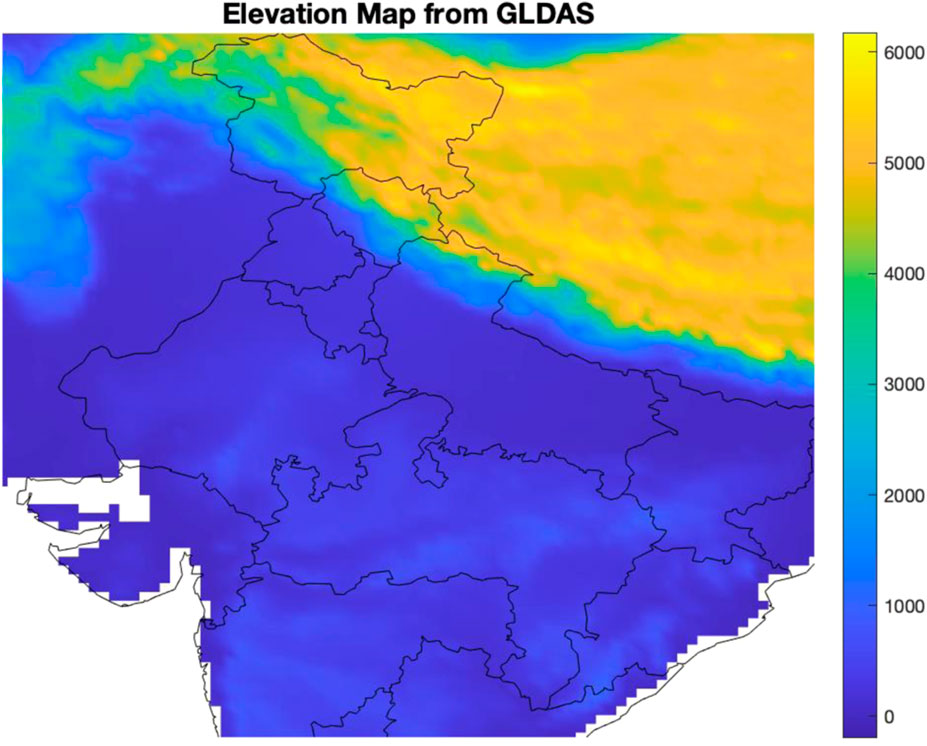
FIGURE 1. Elevation map of North India from the Global Land Data Assimilation System (Rodell et al., 2004).
The climate of North India is heavily influenced by its geographical position and topography. As a subcontinent, it experiences distinct seasons due to its proximity to the equator. The presence of the Himalayas in the north plays a crucial role in moderating temperatures by blocking the intrusion of cold air into the lowlands. Consequently, the climate varies significantly from the plains of Uttar Pradesh to the mountainous regions of Himachal Pradesh and Uttarakhand. The region encounters frigid winters, scorching summers, and mild monsoons. Being one of the most climatically diverse regions on Earth, North India has witnessed a significant rise in mean annual temperatures in several areas, including the west coast, interior peninsula, north-central, and northeastern regions of the country. This warming trend is primarily attributed to the post-monsoon and winter seasons.
In the plains (Punjab, Haryana, Rajasthan, and Uttar Pradesh), the region receives substantial rainfall, while the Himalayas (J.K., H.P., and Uttarakhand) experience snowfall. The northern portion of India’s annual mean temperatures has shown a modest but discernible warming trend, largely influenced by the post-monsoon and winter seasons (Kumar et al., 2023; Rani, 2023).
2.2 Data
Historical and future climate data were sourced from the sixth Coupled Model Inter-comparison Project (Eyring et al., 2016; McBride et al., 2021; Tebaldi et al., 2021). This study focuses on the performance evaluation of 12 CMIP6 models over North India. The selected models are listed in Table 1 along with their host institutions and abbreviations used in this research. The criterion for selecting these models was their availability of model projections.
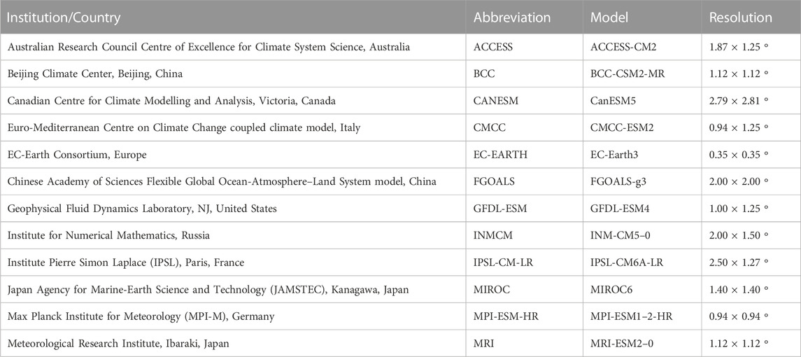
TABLE 1. Detailed description of the CMIP6 GCMs used in this research.
To access the model output, data were downloaded from the open-access platform (https://esgf-node.llnl.gov), which provides historical and future projections of monthly surface temperature. The chosen variant label for CMIP6 is r1i1p1f1, simplifying the evaluation process. The study also utilizes new Shared Socioeconomic Pathways (SSPs), considering potential changes in the Earth’s environment, as well as global economic and demographic trends. Specifically, the study focuses on the future projections of radiative forcing in CMIP6, using SSP5-8.5.
The model simulations cover the period from 1860 to 2100, and the historical period of simulation is divided into two sub-periods: the pre-industrial period (1870–1900) and the present-day climate (1976–2005). Historical simulations are driven by observed atmospheric composition changes, including Greenhouse Gas (GHG), natural and anthropogenic aerosols, volcanic forcing, solar variations, and time-evolving land cover, aiming to simulate the observed climate of the recent historical period. On the other hand, projected climate simulations consider changes in GHGs, solar constant, ozone, and aerosols over time.
For model evaluation, Climatic Research Unit (CRU) gridded rainfall and temperature data (Harris et al., 2014) with 0.5° grid resolution at land points are used. The models are validated for the present period. To compare the model outputs against CRU observations, CMIP6 data at coarser resolution are interpolated to match the finer resolution of CRU data on a 0.5° × 0.5° grid. The multi-model ensemble is calculated in a similar manner. Interannual variations are computed by creating masks for corresponding states, and then averaging the grid points within each mask. For future projections analysis, the model resolution is used without any interpolation.
3 Result and discussion
The findings have been sorted down into two main areas for more in-depth analysis: first, the model validation for the reference period, and second, the forecasts for different climate scenarios. The model simulations were validated in terms of climatology and interannual time series against the corresponding observations. In addition, the climate change in the two future scenarios relative to the preindustrial and the present scenario has been thoroughly analyzed. Annual temperature projections and heat maps are considered for this purpose. Additionally, the return period for temperature events is analysed. The results are focused on the study region which consists of the following states (a) Haryana, (b) Himachal Pradesh, (c) Jammu & Kashmir, (d) Punjab (e) Rajasthan, (f) Uttar Pradesh, and (g) Uttarakhand. Surface temperature plays an important role in numerous disciplines, including weather forecasting, ecology, and environmental monitoring. Along with thermometers and infrared thermometers, now satellite remote sensing data are used in research and evaluation systems. Long-term inferences can be drawn by analyzing surface temperature patterns over time, such as rising temperatures associated with global warming or localized temperature variations resulting from land-use changes or pollution. The coming section deals with the model validation against the corresponding observations through climatological spatial maps and interannual time series for the present period.
3.1 Model validation
In the backdrop of evaluating the proficiency of climate models, we delved into assessing the climatology and interannual variability skills of the CMIP6 models. This validation process provided a pivotal groundwork for ensuring the accuracy and reliability of our subsequent analyses. Our focus was centered on representing the temporal and spatial characteristics of surface temperature across the northern states of India during the designated reference period.
The temperature climatology over the northern states of India is analyzed for reference period using the surface temperature derived from CMIP6 and CRU. Figure 2 represents the climatology of surface temperature from CRU observation (left panel) and CMIP6 ensemble means (middle panel) for the baseline period (1991–2015). The right-hand panel represents the bias between the model and observation It is observed from Figures 2A, B that the temperature of the plain region lies near 25°C and the Himalayan region near to 6°C. In Figure 2C, biases are evaluated between the CRU and CMIP6 data set, where white patches depict a small difference of
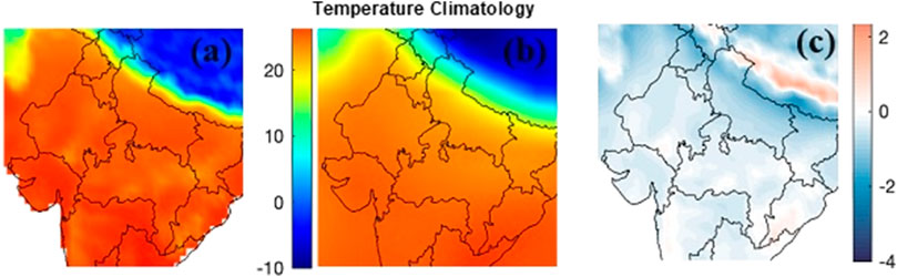
FIGURE 2. Mean surface temperature from (A): Climatic Research Unit (CRU) observation (left panel), (B): CMIP6 ensemble mean (middle panel) for the base line period (1991–2015) and (C): the right-hand panel represents the bias between the model and observation.
In-depth analysis has been conducted to evaluate the proficiency of CMIP6 models at the interannual scale across the northern Indian states spanning from 1986 to 2015. Figure 3 vividly presents the surface temperature data, with the CRU-recorded values represented by the black line, and the simulated data derived from the ensemble mean of CMIP6 models showcased as the green line. This representation encompasses seven Indian states.
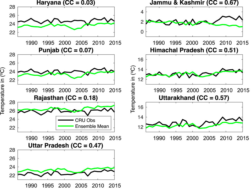
FIGURE 3. Interannual surface temperature variability illustrated by the Climatic Research Unit (CRU) observational dataset (black line) and the ensemble mean of CMIP6 Models (green line) across various states during the timeframe of 1986–2015. The corresponding Correlation Coefficient (CC) value between the model and observation is provided adjacent to each state’s name.
It is of particular note that a significant correlation peak (CC = 0.67) is discerned between these two datasets, notably observed over Jammu and Kashmir (J.K.), while the least correlation is evident in the case of Haryana (CC = 0.03). Interestingly, the correlation dynamics between observed and modelled values exhibit greater cohesion within the Himalayan region compared to the plains, with a notable deviation in the case of Uttar Pradesh (U.P.). Astonishingly, Uttar Pradesh demonstrates a correlation coefficient (nearly 0.5) akin to that of the Himalayan states, even though its geographical classification places it within the plains. This intriguing alignment might stem from the geographical proximity of Uttar Pradesh to the Himalayan states, implying the potential influence of neighbouring regions.
The observed variations and deviations in correlation across timeframes are likely influenced by a confluence of factors, encompassing stochastic variations, external events, regional geography, and inherent uncertainties inherent to measurement and simulation processes. This intricate interplay underscores the multifaceted nature of climate dynamics and underscores the imperative for comprehensive investigation into the intricate interactions between localized variables and model performance.
3.2 Future projection of temperature
In this section, we delve into the future projection of temperature, as captured by the ensemble mean of the models. Figure 4 serves as a comprehensive visual representation, encompassing mean temperatures across all scenarios and their variations relative to the preindustrial period.
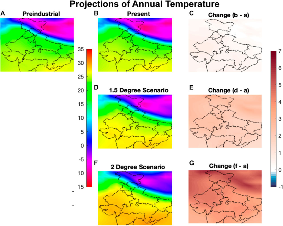
FIGURE 4. Annual mean temperature (°C) as ensemble mean CMIP6 models during the (A): preindustrial period, (B): Present period, and projected in the (D): 1.5°C and (F): 2°C e scenarios. The right-hand side panels show the corresponding projected changes (C, E, G): with respect to the preindustrial period.
The right column of the figure specifically focuses on projected changes, delineating the temperature differences between various scenarios and the preindustrial baseline. Figure 4C notably depicts a minimal temperature change during the present reference period, suggesting a gradual temperature increase during this timeframe. Further, we observe a temperature change of approximately 3°C during the 1.5°C scenario compared to the preindustrial era, slightly exceeding the changes observed in the present scenarios presented in Figure 4C.
A notable observation surfaces in Figure 4G, illustrating a maximum temperature change of about 4.5°C when comparing the 2°C scenario to the preindustrial period. Sequentially analyzing the right columns from top to bottom reveals consistent differences of approximately 1.5°C between consecutive scenarios.
The pivotal insight gleaned from Figure 4 is that the most substantial rise in temperature concerning the preindustrial baseline is observed in the 2°C scenario, accentuating this scenario’s heightened impact on the region’s temperature dynamics. This comprehensive depiction underscores the range of potential temperature shifts under various scenarios, offering critical insights into the potential future climate trajectory.
One of the studies in South Asia, projected largest temperature changes in India by 1.0°C–4.2°C at the end of the twenty-first century. Under the SSP5-8.5 scenario, North India is likely to experience the largest increase in temperature up to 6°C by the end of the twenty-first century. Additionally, the uncertainty in temperature ranges from 0.8°C to 5.4°C in different SSP scenarios (Almazroui et al., 2020). The observed increase was known to cause by external forcings, including GHGs and land use change (Basha et al., 2017).
To gain deeper insights into the temperature dynamics across different climate scenarios and time periods within the seven northern Indian states, we carried out a comprehensive comparison through a box and whiskers plot, designed to visualize the temperature variation. Figure 5 depicts the ensemble mean spread, medians, Interquartile (IQ) ranges, and outliers for the temperature difference across seven northern Indian states at preindustrial, present, and two warming levels of 1.5 and 2
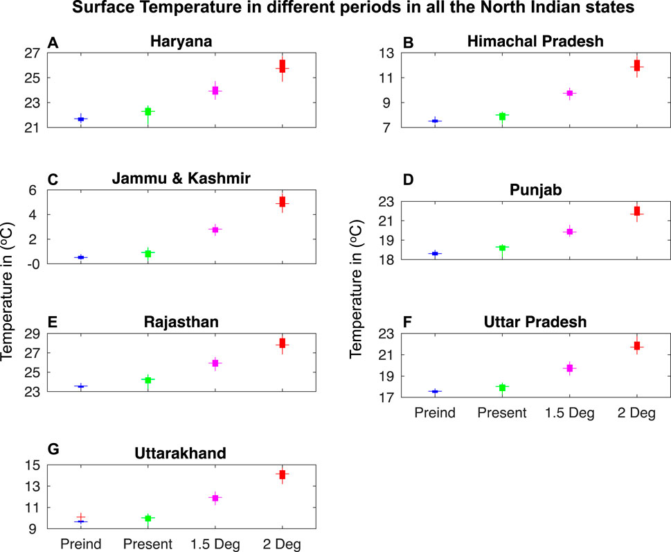
FIGURE 5. Comparison of surface temperature in Preindustrial period, Present Period, 1.5°C Scenario and 2.0°C Scenario as simulated by CMIP6 Models over (A) Haryana, (B) Himachal Pradesh, (C) Jammu & Kashmir, (D) Punjab (E) Rajasthan, (F) Uttar Pradesh and (G) Uttarakhand through box-whisker plot.
Maximum temperature rise is observed in the 2°C scenario and it is interesting to calculate the percentage rise in temperature by considering 2°C scenario in different states and locating the most affected state in terms of temperature rise. After calculating the percentage increase in temperature with respect to the present period (Figure 5), it is observed that the maximum increase observed is 400% for J.K, 50% for H.P., and 40% for Uttarakhand respectively. This clearly signifies that Himalayan regions are affected the most particularly for J.K. state. In one of the earlier studies, the CMIP5 model predicted that the Himalayan region is projected to face higher extreme temperatures by the end of the 21st century under RCP8.5 emission scenarios. Additionally, the projected mean warming over India will be in the range of 3.3°C–4.8°C by the 2080s, relative to the preindustrial period which are in accordance with current interpretation (Chaturvedi et al., 2012).
The Intergovernmental Panel on Climate Change (IPCC) predicts an average temperature increase of 3.3°C for South Asia by the mid-twenty-first century, with temperatures potentially rising by more than 2°C over land in most South Asian countries. The frequency of extreme heatwaves associated to extreme temperature are also expected to increase in South Asia (Ganeshi et al., 2023), leading to severe drought conditions and impacting agriculture and water availability. However not only for South Asia, major land regions of the world have been exhibiting a severe rise in temperature extremes during the past few decades (Perkins et al., 2012). Increases in night-time temperatures and warmest daytime temperatures have been observed at most weather stations across Nepal, India, Sri Lanka, and Pakistan (Naveendrakumar et al., 2019).
Our exploration continues with Figure 6, an intricate heatmap that meticulously charts the surface temperature dynamics across multiple scenarios and timeframes within seven distinct northern Indian states. These states—Haryana, Himachal Pradesh, Jammu & Kashmir, Punjab, Rajasthan, Uttar Pradesh, and Uttarakhand—serve as focal points for this intricate analysis. This captivating visualization, featured in Figure 6, unfolds as a heat map. It aptly portrays the surface temperature landscape across critical periods: the Preindustrial period, the Present Period, the 1.5°C Scenario, and the 2.0°C Scenario, each simulated by CMIP6 Models. The color spectrum’s gradient, ranging from reddish hues symbolizing higher values to cooler blueish shades indicating lower values, provides an immediate overview of temperature variations.
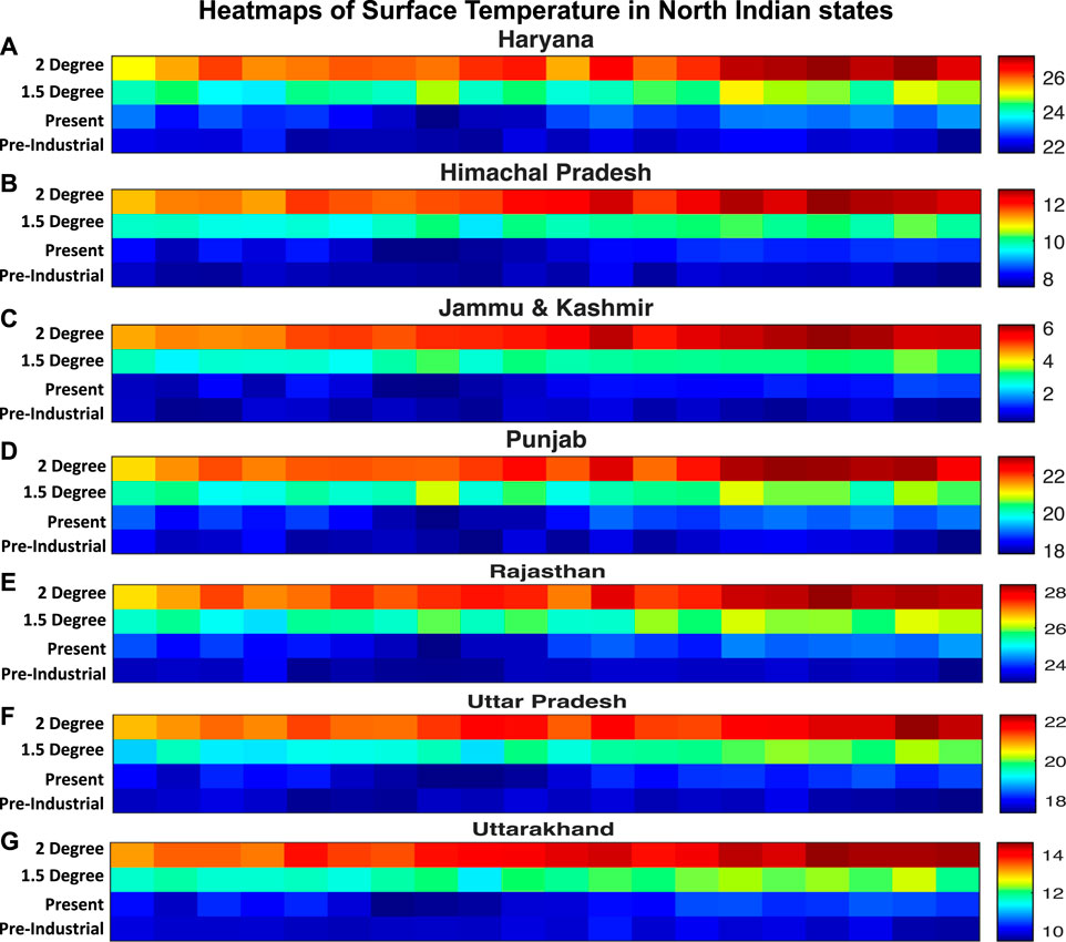
FIGURE 6. Heatmap of surface temperature in the Preindustrial period, Present Period, 1.5°C Scenario and 2.0°C Scenario as simulated by CMIP6 Models over (A) Haryana, (B) Himachal Pradesh, (C) Jammu & Kashmir, (D) Punjab, (E) Rajasthan, (F) Uttar Pradesh and (G) Uttarakhand.
Upon close scrutiny of the color distribution, intriguing patterns emerge. In the Himalayan region, specifically Jammu & Kashmir (J.K.), the lowest temperature is discernible in the 2.0°C Scenario. Comparatively, among the states in the plain region, Rajasthan exhibits the lowest temperature in the 2.0°C Scenario. Interestingly, Haryana and Punjab exhibit a similar temperature variation in the 2.0°C Scenario, with the highest temperature observed in Uttar Pradesh (U.P.) within the plain region.
Both the heatmap and the earlier discussed box-whiskers plot unambiguously portray a consistent temperature rise within the 2.0°C Scenario. This observation echoes findings from other reputable sources (Kumar et al., 2021), reinforcing the notion of a discernible warming trend across the northwest and central regions of Northern India. The study found that the maximum temperature index showed a positive trend predominantly across India (Kumar et al., 2021). It suggests that India can expect an increase in both maximum temperature and the frequency of hot days and nights in the future. A notable exception in the lower Himalayan region and some parts of Uttarakhand are observed which may be dependent on various other factors such as monsoons, topography, seasonal variations, air masses, and urbanization.
3.3 Return periods of temperature extremes
The temperature return period diagram depicts the frequency and severity of critical temperature occurrences over a certain time period. This is done by sorting historical temperature data from highest to lowest and computing the return period for each temperature value. Figure 7 represents the return level of extreme temperature events for all seven states in the preindustrial period, present period, 1.5
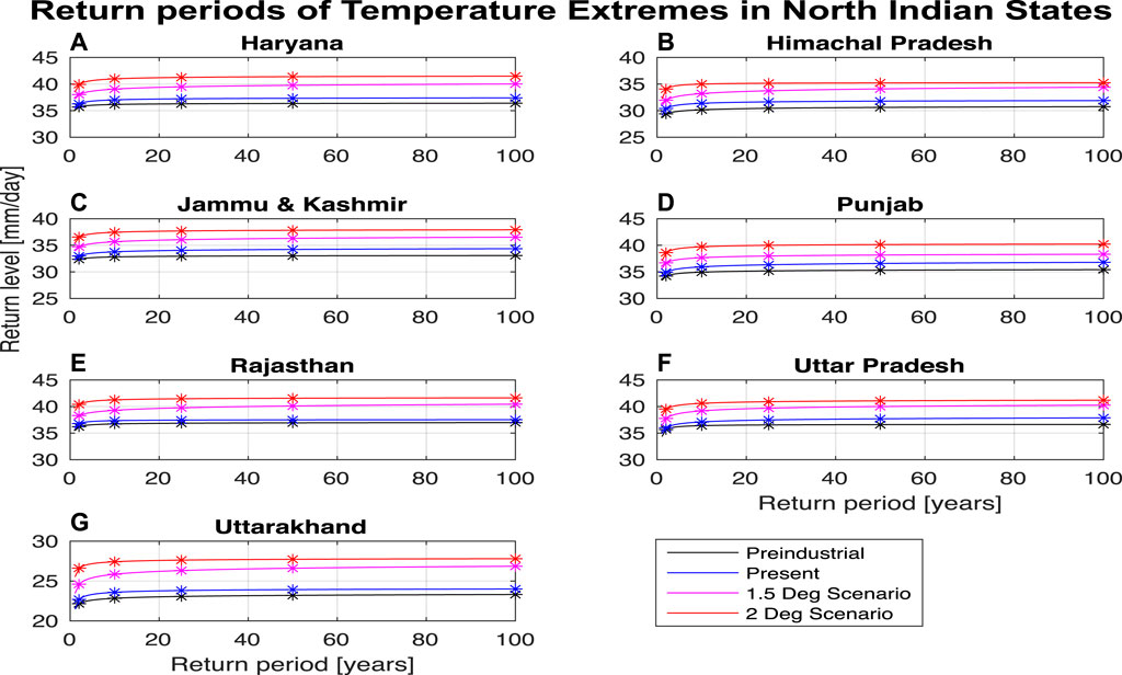
FIGURE 7. Return period of extreme temperature events in the Preindustrial period, Present Period, 1.5°C and 2.0°C Scenario as simulated by CMIP6 Models over (A) Haryana, (B) Himachal Pradesh, (C) Jammu & Kashmir, (D) Punjab, (E) Rajasthan, (F) Uttar Pradesh and (G) Uttarakhand.
Analysis reveals that the predominance of temperature estimates higher than 22°C in all the return periods. It is interesting to understand the relationship between the return time and recurrence level of temperature which shows almost similar behavior for all the states of the Himalayan as well plain region. For the plain region, return level of more than 23°C, which can approach 40°C during a 60-year period is observed. It is observed that the temperature recurrence level increases in all states and reaches a maximum of 37
One of the studies suggest that the joint behaviour of climate extremes across India for past and future periods under RCP4.5 with respect to 2025–2055, depicts that the whole country has negative trend of return period for maximum and minimum temperature extremes during 1985 to 2016 (Kumar et al., 2021). This study suggests that the frequency of extreme temperature events is decreasing across the country during this period. However, the frequency of extreme temperature events is decreasing in fewer regions during the period 2065–2095 (Kumar et al., 2021). Ullah et al. (2022) observed that the frequency of 50-year temperature extreme events could spike to 25–60 times the current return period under 2°C warming. Moreover, in the moderate emissions scenario (SSP2-4.5), as temperature duration and severity rises, there is also a trend of increasing return periods (Ullah et al., 2022). Vieira et al., 2023 stated that for a temperature of 20-year return periods, the highest value was 47.02°C and the lowest value was 34.33°C. For the 50-year return period, the maximum temperature rose to 47.21°C and the minimum increased to 34.60°C (Vieira et al., 2023).
4 Conclusion
This study utilizes CMIP6 ensembles to assess projected fluctuations in surface temperature in the states of North India. The validation of CMIP6 ensemble mean temperature climatology for the reference period (1976–2015) using CRU measurements demonstrates a strong correlation greater than 0.5 significant at 0.01 in 4 out of 7 countries. The analysis focuses on four periods: preindustrial, present, 1.5°C, and 2°C scenarios, using 12 selected CMIP6 models capable of simulating different aspects of temperature and its associated mechanisms.
The results reveal an overall rising tendency of temperature in all states, particularly in the Himalayan region. The maximum temperature rise is observed under the 2°C scenario, with Jammu and Kashmir depicting the least temperature increase and Rajasthan showing the highest. The Himalayan regions experience a more significant temperature rise compared to the plain regions, with Jammu and Kashmir being particularly affected. Analysis of temperature return periods indicates predominance of estimates higher than 22°C across 60-year return periods. Uncertainties exist in GCM-simulated temperature across the examined region, with variations of about ±0.5°C. Inter-model comparisons show that CMIP6 model projections are generally more reliable at global scales than at smaller scales.
Despite providing valuable insights, this study has limitations, notably the coarse resolution, which affects uncertainty reduction at the regional level. Quantifying model errors and uncertainties is crucial for improving future estimates. Enhancing model performance over vast regions will aid in developing effective mitigation strategies to reduce temperature rise and minimize negative repercussions on the region. In the long run, focusing on developing and refining model performance globally will contribute to better climate research, facilitating the formulation of impactful mitigation strategies. Understanding temperature variability is essential in detecting abnormal changes and ensuring the stability of this critical climate variable. By addressing these challenges, we can work towards safeguarding North India’s environment and its inhabitants from the impacts of climate change.
Data availability statement
Publicly available datasets were analyzed in this study. This data can be found here: All data used in this study are freely available and can be requested from the authors or obtained directly from the source: CRU data (http://www.cru.uea.ac.uk/data), and CMIP6 data (https://esgf-node.llnl.gov).
Author contributions
AA: Conceptualization, Formal Analysis, Project administration, Resources, Supervision, Writing–original draft, Writing–review and editing. KP: Conceptualization, Data curation, Formal Analysis, Funding acquisition, Investigation, Methodology, Project administration, Resources, Software, Validation, Visualization, Writing–review and editing. AT: Writing–review and editing. AS: Writing–review and editing. MC: Writing–review and editing.
Funding
The authors declare that no financial support was received for the research, authorship, and/or publication of this article.
Acknowledgments
All the authors acknowledge CMIP6, CRU for providing the climate data. KP acknowledge the support from the NERC (UK Natural Environment Research Council) AMAZONICA and Amazon Hydrological Cycle grants (NE/F005806/1 and NE/K01353X/1). AA thankful to the University of Petroleum and Energy Studies, Dehradun for providing research facilities.
Conflict of interest
Author MC was employed by LEA Associates South Asia Pvt. Ltd.
The remaining authors declare that the research was conducted in the absence of any commercial or financial relationships that could be construed as a potential conflict of interest.
Publisher’s note
All claims expressed in this article are solely those of the authors and do not necessarily represent those of their affiliated organizations, or those of the publisher, the editors and the reviewers. Any product that may be evaluated in this article, or claim that may be made by its manufacturer, is not guaranteed or endorsed by the publisher.
References
Almazroui, M., Saeed, S., Saeed, F., Islam, M. N., and Ismail, M. (2020). Projections of precipitation and temperature over the South Asian countries in CMIP6. Earth Syst. Environ. 4 (2), 297–320. doi:10.1007/s41748-020-00157-7
Awasthi, A., Dewan, R., and Singh, G. (2022a). “Glacier melting: Drastic future,” in Advances in behavioral based safety. Editors N. A. Siddiqui, F. Khan, S. M. Tauseef, W. S. Ghanem, and V. Garaniya (Berlin, Germany: Springer Nature), 255–266. doi:10.1007/978-981-16-8270-4_19
Awasthi, A., Sharma, A., Kaur, P., Gugamsetty, B., and Kumar, A. (2021). Statistical interpretation of environmental influencing parameters on COVID-19 during the lockdown in Delhi, India. Environ. Dev. Sustain. 23 (6), 8147–8160. doi:10.1007/s10668-020-01000-9
Awasthi, A., Vishwakarma, K., and Pattnayak, K. C. (2022b). Retrospection of heatwave and heat index. Theor. Appl. Climatol. 147 (1), 589–604. doi:10.1007/s00704-021-03854-z
Basha, G., Kishore, P., Ratnam, M. V., Jayaraman, A., Agha Kouchak, A., Ouarda, T. B. M. J., et al. (2017). Historical and projected surface temperature over India during the 20th and 21st century. Sci. Rep. 7 (1), 2987. doi:10.1038/s41598-017-02130-3
Beusch, L., Nauels, A., Gudmundsson, L., Gütschow, J., Schleussner, C.-F., and Seneviratne, S. I. (2022). Responsibility of major emitters for country-level warming and extreme hot years. Commun. Earth Environ. 3 (1), 7. doi:10.1038/s43247-021-00320-6
Brun, A. (2016). Conference diplomacy: The making of the Paris agreement. Polit. Gov. 4 (3), 115–123. doi:10.17645/pag.v4i3.649
Chaturvedi, R., Joshi, J., Jayaraman, M., Govindasamy, B., and Ravindranath, N. H. (2012). Multi-model climate change projections for India under representative concentration pathways. Curr. Sci. 103, 791–802.
Das, J., Manikanta, V., and Umamahesh, N. V. (2022). Population exposure to compound extreme events in India under different emission and population scenarios. Sci. Total Environ. 806, 150424. doi:10.1016/j.scitotenv.2021.150424
Eyring, V., Bony, S., Meehl, G. A., Senior, C. A., Stevens, B., Stouffer, R. J., et al. (2016). Overview of the coupled model Intercomparison project Phase 6 (CMIP6) experimental design and organization. Geosci. Model Dev. 9 (5), 1937–1958. doi:10.5194/gmd-9-1937-2016
Fragkos, P., Laura van Soest, H., Schaeffer, R., Reedman, L., Köberle, A. C., Macaluso, N., et al. (2021). Energy system transitions and low-carbon pathways in Australia, Brazil, Canada, China, EU-28, India, Indonesia, Japan, Republic of Korea, Russia and the United States. Energy 216, 119385. doi:10.1016/j.energy.2020.119385
Ganeshi, N. G., Mujumdar, M., Yuhei, T., Goswami, M. M., Singh, B. B., Krishnan, R., et al. (2023). Soil moisture revamps the temperature extremes in a warming climate over India. Npj Clim. Atmos. Sci. 6 (1), 12. doi:10.1038/s41612-023-00334-1
Harris, I., Jones, P. d., Osborn, T. j., and Lister, D. h. (2014). Updated high-resolution grids of monthly climatic observations – The CRU TS3.10 dataset. Int. J. Climatol. 34 (3), 623–642. doi:10.1002/joc.3711
Karstensen, J., Roy, J., Pal, B., Peters, G., and Andrew, R. (2020). Key drivers of Indian greenhouse gas emissions. Econ. Political Wkly. 55, 46–53.
Kaul, M., Dadhwal, V. K., and Mohren, G. M. J. (2009). Land use change and net C flux in Indian forests. For. Ecol. Manag. 258 (2), 100–108. doi:10.1016/j.foreco.2009.03.049
Kirkpatrick, S. E. P., and Lewis, S. C. (2020). Increasing trends in regional heatwaves | Nature Communications. Available at: https://www.nature.com/articles/s41467-020-16970-7.
Kumar, H., and Tiwari, S. (2023). Climatology, trend of aerosol-cloud parameters and their correlation over the Northern Indian Ocean. Geosci. Front. 14 (4), 101563. doi:10.1016/j.gsf.2023.101563
Kumar, N., Kumar Goyal, M., Kumar Gupta, A., Jha, S., Das, J., and Madramootoo, C. A. (2021). Joint behaviour of climate extremes across India: Past and future. J. Hydrology 597, 126185. doi:10.1016/j.jhydrol.2021.126185
Lal, M., and Singh, R. (2000). Carbon sequestration potential of Indian forests. Environ. Monit. Assess. 60 (3), 315–327. doi:10.1023/A:1006139418804
McBride, L. A., Hope, A. P., Canty, T. P., Bennett, B. F., Tribett, W. R., and Salawitch, R. J. (2021). Comparison of CMIP6 historical climate simulations and future projected warming to an empirical model of global climate. Earth Syst. Dyn. 12 (2), 545–579. doi:10.5194/esd-12-545-2021
McClymont, H., and Hu, W. (2021). Weather variability and COVID-19 transmission: A review of recent research. Int. J. Environ. Res. Public Health 18 (2), 396. doi:10.3390/ijerph18020396
Mecenas, P., Bastos, R. T., Vallinoto, A. C. R., and Normando, D. (2020). Effects of temperature and humidity on the spread of COVID-19: A systematic review. PLOS ONE 15 (9), e0238339. doi:10.1371/journal.pone.0238339
Naveendrakumar, G., Vithanage, M., Kwon, H.-H., Chandrasekara, S. S. K., Iqbal, M. C. M., Pathmarajah, S., et al. (2019). South asian perspective on temperature and rainfall extremes: A review. Atmos. Res. 225, 110–120. doi:10.1016/j.atmosres.2019.03.021
Parry, I. W. H., Black, M. S., Minnett, D. N., Mylonas, M. V., and Vernon, N. (2022). How to cut methane emissions. International Monetary Fund.
Pattnayak, K. C., Awasthi, A., Sharma, K., and Pattnayak, B. B. (2023). Fate of rainfall over the North Indian states in the 1.5 and 2°C warming scenarios. Earth Space Sci. 10 (2), e2022EA002671. doi:10.1029/2022EA002671
Perkins, S. E., Alexander, L. V., and Nairn, J. R. (2012). Increasing frequency, intensity and duration of observed global heatwaves and warm spells. Geophys. Res. Lett. 39 (20). doi:10.1029/2012GL053361
Raghavan, K., Sanjay, J., Gnanaseelan, C., Mujumdar, M., Kulkarni, A., and Chakraborty, S. (2020). Assessment of climate change over the Indian region A report of the ministry of Earth sciences (MoES), government of India: A report of the ministry of Earth sciences (MoES), government of India. Berlin, Germany: Springer. doi:10.1007/978-981-15-4327-2
Rani, S. (2023). “Climate variability assessment,” in Climate, land-use change and hydrology of the beas river basin, western Himalayas (Cham: Springer International Publishing), 101–135.
Riahi, K., van Vuuren, D. P., Kriegler, E., Edmonds, J., O’Neill, B. C., Fujimori, S., et al. (2017). The Shared Socioeconomic Pathways and their energy, land use, and greenhouse gas emissions implications: An overview. Glob. Environ. Change 42, 153–168. doi:10.1016/j.gloenvcha.2016.05.009
Rodell, M., Houser, P. R., Jambor, U., Gottschalck, J., Mitchell, K., Meng, C.-J., et al. (2004). The global land data assimilation system. Bull. Am. Meteorological Soc. 85 (3), 381–394. doi:10.1175/BAMS-85-3-381
Rose, S. K., Richels, R., Blanford, G., and Rutherford, T. (2017). The Paris Agreement and next steps in limiting global warming. Clim. Change 142 (1), 255–270. doi:10.1007/s10584-017-1935-y
Shakil, M. H., Munim, Z. H., Tasnia, M., and Sarowar, S. (2020). COVID-19 and the environment: A critical review and research agenda. Sci. Total Environ. 745, 141022. doi:10.1016/j.scitotenv.2020.141022
Singh, A., Srivastava, A. K., Pathak, V., and Shukla, A. K. (2022). Quantifying the impact of biomass burning and dust storm activities on aerosol characteristics over the Indo-Gangetic Basin. Atmos. Environ. 270, 118893. doi:10.1016/j.atmosenv.2021.118893
Singh, J. S., and Chaturvedi, R. K. (2017). Diversity of ecosystem types in India: A review. Proc. Indian Natl. Sci. Acad. 83 (2), 569–594. doi:10.16943/ptinsa/2017/49027
Tebaldi, C., Debeire, K., Eyring, V., Fischer, E., Fyfe, J., Friedlingstein, P., et al. (2021). Climate model projections from the scenario model Intercomparison project (ScenarioMIP) of CMIP6. Earth Syst. Dyn. 12 (1), 253–293. doi:10.5194/esd-12-253-2021
Ullah, I., Ma, X., Asfaw, T. G., Yin, J., Iyakaremye, V., Saleem, F., et al. (2022). Projected changes in increased drought risks over South Asia under a warmer climate. Earth’s Future 10 (10), e2022EF002830. doi:10.1029/2022EF002830
Vieira, F., Oliveira, M., Sanfins, M., Garção, E., Dasari, H., Dodla, V., et al. (2023). Statistical analysis of extreme temperatures in India in the period 1951–2020. Theor. Appl. Climatol. 152, 473–520. doi:10.1007/s00704-023-04377-5
Keywords: climate model, CMIP6, North India, return period, temperature trends
Citation: Awasthi A, Pattnayak KC, Tandon A, Sarkar A and Chakraborty M (2023) Implications of climate change on surface temperature in North Indian states: evidence from CMIP6 model ensembles. Front. Environ. Sci. 11:1264757. doi: 10.3389/fenvs.2023.1264757
Received: 21 July 2023; Accepted: 04 September 2023;
Published: 20 September 2023.
Edited by:
Rosaria Costa, University of Messina, ItalyReviewed by:
Bogdan Bochenek, Institute of Meteorology and Water Management, PolandSerena Savoca, University of Messina, Italy
Claudio D’Iglio, University of Messina, Italy, in collaboration with reviewer SS
Copyright © 2023 Awasthi, Pattnayak, Tandon, Sarkar and Chakraborty. This is an open-access article distributed under the terms of the Creative Commons Attribution License (CC BY). The use, distribution or reproduction in other forums is permitted, provided the original author(s) and the copyright owner(s) are credited and that the original publication in this journal is cited, in accordance with accepted academic practice. No use, distribution or reproduction is permitted which does not comply with these terms.
*Correspondence: Kanhu Charan Pattnayak, k.c.pattnayak@leeds.ac.uk; Amit Awasthi, awasthitiet@gmail.com