
94% of researchers rate our articles as excellent or good
Learn more about the work of our research integrity team to safeguard the quality of each article we publish.
Find out more
ORIGINAL RESEARCH article
Front. Environ. Sci., 08 November 2023
Sec. Environmental Informatics and Remote Sensing
Volume 11 - 2023 | https://doi.org/10.3389/fenvs.2023.1253949
 Benli Guo1,2,3,4
 Shouchuan Zhang5*Kai Liu5*Peng Yang1,2,3,4Honglian Xing1,2,3,4Qiyuan Feng1,2,3,4Wei Zhu1,2,3,4
 Yaoyao Zhang5Wuhui Jia5
The excessive exploitation of groundwater not only destroys the dynamic balance between coastal aquifer and seawater but also causes a series of geological and environmental problems. Groundwater level prediction provides an efficient way to solve these intractable ecological problems. Although several hydrological numerical models have been employed to conduct prediction, no study has accurately predicted the groundwater level change under the consideration of groundwater exploitation, especially in coastal aquifers. This is due to the characteristics of spatially and temporally complex hydrological processes. This study proposes a novel data-driven method based on the combination of time series analysis and a machine learning method for accurately predicting the variation of groundwater level in a coastal aquifer under the influence of groundwater exploitation. The partial autocorrelation function and continuous wavelet coherence were used to analyze the monitoring data of groundwater level at three wells, which indicated that the historical monitored data and the dataset of precipitation could be considered as the input variables to construct the hydrological model. Then, three models based on the different inputs were constructed, namely, the LSTM, PACF-LSTM, and PACF-WC-LSTM models. The performances of the three models were compared by the calculation of four error metrics. The results showed that the performance of the PACF-LSTM and PACF-WC-LSTM models was better than that of the LSTM model and that the PACF-WC-LSTM model achieved the best prediction performance. Accurately predicting the variation of groundwater level provides the basis for managing groundwater resources and preserving the ecological environment.
Groundwater is the most important resource for supporting the demand from agriculture and industrial and domestic water supplies, and it also plays a crucial role in maintaining the stability of the ecosystem (Hu et al., 2019; Xiao et al., 2022; Hikouei et al., 2023). Over a quarter of the population across the world depends on groundwater resources as their primary water resource, and more than half of irrigation water in agriculture is supplied by groundwater resources (WWAP, 2015). However, due to rapid urbanization and intensified human activities, the overexploitation of groundwater resources causes a series of intractable environmental problems (Long et al., 2020), such as geological disaster (Hosono et al., 2019; Miyakoshi et al., 2020; Qu et al., 2020), land subsidence (Wang et al., 2013; Xiao et al., 2022; Hikouei et al., 2023), and land desertification (Daliakopoulos et al., 2005; Qu et al., 2021; Sun et al., 2022). Moreover, the intensive exploitation of groundwater induces an imbalance between the surface water, groundwater, and seawater in coastal regions, which causes saltwater intrusion and land salinization (Tokunaga, 1999; Lee et al., 2013; Nourani et al., 2014; Wang et al., 2023). Thus, it is extremely urgent to solve these difficult environmental problems caused by the overexploitation of groundwater resources.
The scientific monitoring and accurate prediction of groundwater levels have focused on solving these intractable environmental problems and providing the basis for the implementation of effective management of groundwater resources (Hosono et al., 2019; Mao et al., 2022; Mohammed et al., 2022). In general, the dynamic change of groundwater level is affected by external influencing factors, such as seismic activities, precipitation, and pumping activities (Nourani et al., 2014; Shi et al., 2018; Wang et al., 2018; Gao et al., 2020; Vittecoq et al., 2020). All the external influence factors can be classified into three categories, namely, geological factors, meteorological factors, and anthropogenic factors, which cause groundwater levels to show non-linear dynamic changes in the time domain and frequency domain. The influence of many external factors on groundwater dynamic changes increases the difficulty of groundwater level prediction and decreases the accuracy of prediction. Previous studies have indicated that physical-based models, such as GMS, MODFLOW, and TOUGH, have a predominant advantage for the prediction of groundwater levels in complex hydrogeological conditions (Chen et al., 2020; Tawara et al., 2020; Mohammed et al., 2022). However, these numerical models completely depend on hydrological information, such as stratigraphic structures, aquifer parameters, and boundary conditions. Due to the heterogeneity, discontinuity, and anisotropy of aquifer properties across different scales, hydrological parameters are difficult to obtain accurately. In recent years, data-driven methods have been shown to outperform numerical models in predicting the variation of groundwater level (Kratzert et al., 2018; Bredy et al., 2020; Zhang et al., 2022; Hikouei et al., 2023). The greatest strength of data-driven methods is that these methods can build the relationship between the input variables and target variables without the need to explicitly define physical relationships between them.
Data-driven methods are needed to rebuild the relationship between external influence factors and the variation of groundwater level from a modern perspective. These types of methods have been widely considered to identify anomalous changes in groundwater levels and predict the variation of groundwater levels. Examples of data-driven methods include the decision tree model (Bredy et al., 2020; Zhang et al., 2020), the Hilbert Huang Transform (Zhang et al., 2019; Chien et al., 2020), and the artificial neural network method (Wunsch et al., 2021; Hakim et al., 2022). However, these methods also have major drawbacks. For example, the decision tree method is easy to overfit during the training state, whereas the artificial neural network method cannot quantify how much historical data is used for prediction. n addition, these data-driven groundwater prediction methods do not consider the various external factors that influence the dynamic variation of groundwater level. More recently, the newly developed long short-term memory neural network (LSTM) method has provided an effective way to predict the variation of groundwater level based on valuable data from long-term monitoring and external influencing factors. However, in previous studies, groundwater withdrawal was less considered as the input variable to construct the LSTM model for predicting the variation of groundwater level. In order to improve the accuracy of the prediction model, in the present study, three modified LSTM models with the combination of time series analysis and machine learning methods based on the consideration of groundwater withdrawal were constructed and compared in terms of the performance of groundwater level prediction.
The core objective of this study is to accurately predict the variation of groundwater level under the influence of groundwater exploitation in a coastal area. In accordance with this objective, major research results were achieved by 1) using partial autocorrelation function and continuous wavelet coherence to identify the internal factors and external factors on the variation of groundwater level, and then to determine the input variables of data-driven models; 2) constructing and training three data-driven models, namely, the LSTM model, the PACF-LSTM model, and the PACF-WC-LSTM model, to predict groundwater level; 3) analyzing and comparing the model performance of groundwater level prediction in the validation and prediction stage under four error metrics, namely, R2, MAPE, RMSE, and NSE. Hydrogeologists analyze and predict the variation of groundwater levels, especially those changes under the influence of groundwater exploitation, which can provide the premise for water resource management. However, due to the non-linear and non-stationary characteristics of groundwater level monitored data, there is still no data-driven method to accurately predict groundwater level change under the influence of groundwater exploitation. The result of this study could provide a new data-driven method to simulate and predict groundwater level change under groundwater exploitation in a coastal aquifer.
Rizhao County is located in the Jiaonan uplift of the second-order structural unit, which belongs to the Ludong fault block of the first-order structural unit. Tectonically, it is located in the junction area of the Yishu Fault and the Wurong Fault. The terrain is generally low in the southeast and high in the northwest, and generally increases in height with the increasing distance between the coastline and inland. The length of the coastline in Rizhao County is 168 km. Geomorphic types are divided into three categories: mountain, hill, and plain. The area of hills occupies approximately 57.2% of the city’s territory, whereas the areas of mountains and plains occupy approximately 25.3% and 17.5% of the area, respectively. The main surface water bodies include the Futuan River, Chaobai River, Xiuzhen River, and Wei River, which flow into the Huanghai Sea.
Based on the difference in hydrogeological conditions, the aquifer types in the study area can be roughly classified into four categories: Quaternary loose rock aquifer, Bedrock fissure aquifer, Clastic rock aquifer, and Carbonate rock aquifer (Figure 1). The Quaternary loose rock aquifer is mainly distributed on both sides of the Futuan River and Xiuzhen River and has a wide distribution range and strong water supply capacity. The hydrochemical type in the Quaternary loose rock aquifer is HCO3·Cl-Ca·Na. The Bedrock fissure aquifer is the most widely distributed in the study area, however, its water supply capacity is inadequate. The hydrochemical type in the Bedrock fissure aquifer is HCO3-Ca·Mg. The rock types of the Clastic rock aquifer are composed of conglomerate, siltstone, and clastic rock. The hydrochemical type in the Clastic rock aquifer is HCO3—Ca·Na. The Carbonate rock aquifer is less distributed in the study area.
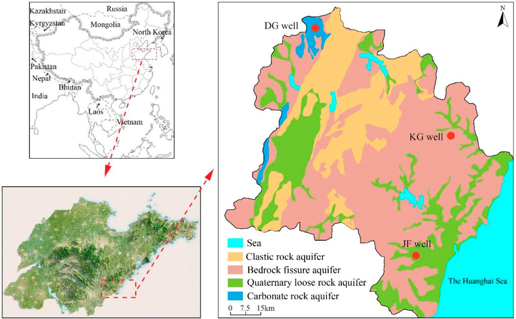
FIGURE 1. The hydrogeological map of Rizhao City and the location of monitoring wells.
Dongguan monitoring well (DG well), Jufeng monitoring well (JF well), and Kouguan monitoring well (KG well) are connected with the Carbonate rock aquifer, Quaternary loose rock aquifer, and Bedrock fissure aquifer, respectively. In this study, the monitored data of groundwater levels in the abovementioned three monitoring wells from 2003 to 2020 were collected to be used in the analysis and prediction of groundwater levels. In addition, precipitation and groundwater withdrawal are important sources of groundwater recharge and discharge, respectively. To accurately analyze and predict groundwater regimes, we also collected the dataset of precipitation and groundwater withdrawal in Rizhao City from 2003 to 2020.
The monitored interval of groundwater levels in these three monitoring wells was 5 days. The dynamic changes in groundwater levels in the three monitoring wells showed seasonal fluctuations, with a higher level during the summer wet season and lower levels during the drier winter season (Figure 2). Due to the difference in hydrological conditions, the magnitude of annual change in groundwater levels showed significant differences: 2.6 m in the DG well, 1.7 m in the JF well, and 3.5 m in the KG well.
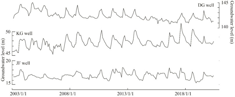
FIGURE 2. The variation of groundwater levels at the three monitoring wells (DG well, KG well, and JF well) from 2003 to 2020.
The meteorological dataset was collected from the China Meteorological Administration (http://data.cma.cn/). Rizhao County is characterized by the monsoon climate of medium latitudes, with a mean annual rainfall of 874 mm, of which approximately 70% falls from June to October. The average value of annual atmospheric temperature is approximately 12.7°C.
The data on groundwater withdrawal in Rizhao was collected from the Rizhao hydrological reports published by the Rizhao Water Resources Bureau (http://slj.rizhao.gov.cn/). As shown in Figure 3, the annual average value of groundwater withdrawal from 2003 to 2020 was 1.595 × 10⁸ m3. The maximum value of groundwater withdrawal was 1.956 × 10⁸ m3 in 2006. Due to the change in water supply structure and effective administration, the amount of annual groundwater withdrawal in Rizhao was reduced to 1.363 × 10⁸ m3 in 2020.
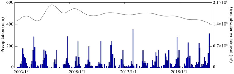
FIGURE 3. The variation of precipitation and groundwater withdrawal from 2003 to 2020.
In order to eliminate the effect of different monitored intervals, the monitored values of groundwater level, precipitation, and groundwater withdrawal were transferred to the monthly average value for analysis.
The partial autocorrelation function (PACF) is an efficiency tool in time series analysis for analyzing the correlation between the Xt and Xt+k by eliminating the variables interference Yt-1, Yt-2, … , Yt− k+1. Partial autocorrelation coefficients can be calculated by the Yule-Walker equation (Tinungki and Iop, 2019; Yan et al., 2021; Zhang et al., 2022; He et al., 2022), as follows:
Where
Partial autocorrelation coefficients can be estimated by using the partial autocorrelation coefficients of the sample by changing the value ρ on the Yule-Walker equation with r, and counting for k = 1, 2, … to get the value Φkk using Cramer rules. Several previous studies indicate that PACF provides an efficient way to analyze the correlation of time series in hydrogeological science (Rodrigues et al., 2018; Yu et al., 2019; Bredy et al., 2020; Nelson et al., 2021; Yan et al., 2021). In this study, we also use this method to analyze the correlation of time series between groundwater level at time t and antecedent groundwater level.
Wavelet transform is an efficient tool to decompose the time series into various times and frequencies and analyze non-stationary time series with multi-time resolution, which mainly includes the discrete wavelet transform (DWT) and the continuous wavelet transform (CWT) (Acworth et al., 2016; Yan et al., 2020; Zhang et al., 2020; Qu et al., 2021). Previous studies indicated that the latter method has been used to analyze the correlation of different hydrological time series (Massei et al., 2006; Nourani et al., 2014; Yan et al., 2017; Lee and Kim, 2019; Zhang et al., 2021). In this study, continuous wavelet coherence was used to identify the external influencing factors of groundwater level change, which is the typical technology in continuous wavelet transform. Due to the perfect performance and good balance in the time and frequency domain, the Morlet wavelet was selected to conduct the continuous wavelet coherence (Massei et al., 2006; Zhang et al., 2022; Gu et al., 2022). Monte Carlo methods were used to determine the statistical significance level of WTC. The Cone of Influence was used to evaluate the edge effects caused by discontinuities at endpoints.
Different from the definition of the correlation coefficient, continuous wavelet coherence is defined as follows:
where the W operator represents the continuous wavelet transform when it has one argument. The capital letter S and lowercase letter s represent the smoothing operator and the wavelet scale, respectively. R2 is the correlation coefficient, which ranges from 0 to 1. The value of 1 means a high correlation between two time series, while the value of 0 means a low correlation between them.
Data-driven artificial neural networks can simulate the data processing process of the human brain. Both recurrent neural networks and long short-term memory are typical artificial neural networks, which are widely used to analyze the non-linear characteristics between input and output variables. The long short-term memory proposed by Hochreiter and Schmidhuber (1997) is the special structure of a recurrent neural network (RNN). Similar to the typical structure of a recurrent neural network, the LSTM network is also composed of three layers: the input layer, the hidden layer, and the output layer. The obvious difference between recurrent neural networks and long short-term memory networks is the algorithm structure of the hidden layer (Rodrigues et al., 2018; Zhang et al., 2022; Zhang et al., 2022; Sun et al., 2022). In recurrent neural networks, the unrolled loop cell is the medium of information transformation, which stores the historical information of time series and allows the historical information to conduct predicting (Wunsch et al., 2021). However, the major drawback of a recurrent neural network is that the unrolled loop cell cannot identify how much historical information should be used to predict the time series. Meanwhile, it also causes vanishing gradients and gradient explosion during the back-propagation. The efficient structure of the hidden layer in the LSTM network, comprising three gates, namely, input gates, output gates, and forget gates, can solve the drawback of the RNN (Zhang et al., 2018; Chen et al., 2021; Vu et al., 2021; Mohammed et al., 2022). The gate structure of the hidden layer controls which historical data in the time series is important to keep and protects the valuable information passed down in the process of information transfer. The distinct structure of the hidden layer can efficiently solve the problem of gradient explosion and gradient disappearance in the training stage (Rodrigues et al., 2018; Yu and Ma, 2021).
Detailed information on the forget gate, input gate, and output gate is introduced as follows:
1) The forget gate can read the stored information in the previous hidden state
Where
2) The input gate identifies what information is to be retained and updated in the cell state, which consists of two layers: the tanh layer and the sigmoid layer. These two layers process the data simultaneously. The tanh layer calculates the update vector based on the last hidden state, and the sigmoid layer determines which historical information can be retained to update the cell state in the current time step. The abovementioned process is defined by the following equation:
Where
3) The output gate determines which historical information can be passed on to the new hidden layer. It is defined by the following equation:
Where Wo is the weight matric and bo is the bias vector.
To improve the accuracy of model prediction, three data-driven models were constructed by machine learning methods: the LSTM model, the PACF-LSTM model, and the PACF-WC-LSTM model. In this section, we introduce how to split the dataset into different stages, how to normalize the dataset, and how to identify the input variables of each model. In the present study, all the modified LSTM models were programmed by MATLAB.
The splitting of the dataset is an important step to train the machine learning model. If the training subset takes up a small proportion, the machine learning model may not analyze and identify the mathematic characteristics of the time series, leading to a reduced accuracy of prediction. If the training and validation subsets take up a large proportion, the model may overfit and lead to data not being accurately predicted. However, there is no fixed ratio between the training dataset, validation dataset, and test dataset (Rodrigues et al., 2018; Wunsch et al., 2021; Zhang et al., 2022). In general, the training dataset should comprise more than 50% of the whole dataset. In this study, the hydrological monitored dataset was split into three subsets: the training subset, the validation subset, and the prediction subset. The proportion of these subsets was 5:3:2. To accurately build the relationship between the input variables and the target variable, the training and validation process is aimed at optimizing the model parameters.
Due to the diversity of monitoring data, the min–max normalization approach was used to normalize all input variables into the range of [0,1], which can improve the learning and training efficiency, and eliminate external influences, especially the dimensional influence. The min–max normalization approach is defined by the following equation:
Where xnorm is the normalized value and x, xmax, and xmin are the monitored value, the maximum monitored value, and the minimum monitored value, respectively. After training, the model output results can be retransformed through the contrary process of Eq. 10.
Four error metrics were selected to evaluate the accuracy and predictive efficiency of the machine learning model, as follows:
The coefficient of determination:
The root mean square error (RMSE):
The mean absolute percentage error (MAPE):
The Nash-Sutcliffe efficiency (NSE):
Where yi is the observed value,
The appropriate input variables provide the basic hydrological information for constructing the hydrological models. Due to the complexity of hydrogeological conditions, there are no guidelines on how to select the input variables for the construction of a hydrological model. The regional groundwater regime is affected by meteorological factors and human activities. In the present study, partial autocorrelation function and continuous wavelet coherence were introduced to identify the influencing factors on the variation of groundwater level and help us select the input variables of the hydrological model. The determination of input variables in each model is introduced in detail in Section 5.3.
The autocorrelation analysis was the efficiency tool used for analyzing the correlation relationship between the hydrological data (d) and the historical time series [d (t-1), d (t-2), …d (t-p)] with p being the lag time. In order to determine whether the historical monitored data of groundwater level data could be considered as an input variable, the autocorrelation analysis was conducted based on the monthly monitored data of groundwater level during the interval of 2003–2020. The partial autocorrelation coefficient of monthly data is shown inFigure 4. The result indicates that the 0th-order partial autocorrelation coefficients are constant at 1. In addition, it is easily found that the autocorrelation coefficients fluctuate around the 0-axis with the increase of lag time, which indicates that the time series of groundwater level in three monitoring wells show the stationary signal.
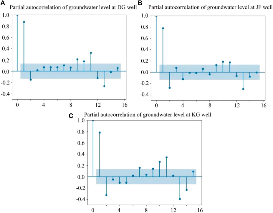
FIGURE 4. Partial autocorrelation coefficient of groundwater level time series in the DG well, KG well, and JF well (Blue solid line is the 95% confidence bound).
For the DG well, the PACF result showed a significant correlation with up to 3 months of lag time for groundwater levels. Hence, the lag time, p, is equivalent to 3 months for groundwater level at the DG well. Similarly, the lag time, p, is also equivalent to 3 months for the groundwater level of the KG well and JF well. The PACF results of three wells indicate that a strong correlation relationship exists between the groundwater level data and the historical monitored data. Thus, the historical dataset of groundwater can be considered as the input variable to predict the target variable.
The wavelet coherence was used to analyze and examine the relationship between the change in groundwater level and the variation of precipitation, which is an efficient time series analysis tool. The coherence relationship between groundwater level and precipitation in three wells is shown in Figure 5. The thick black contour indicates the 95% confidence level. The black arrows indicate the relative phase relationship. The in-phase points to the right, while the anti-phase points to the left. The phase-lagging by 90° points straight up while the phase-leading by 90° points straight down.
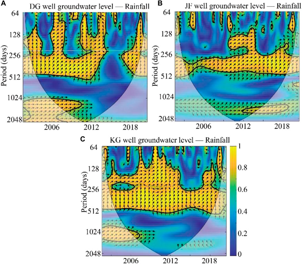
FIGURE 5. Wavelet coherences WTC (1979–2015) between groundwater level and precipitation in (A) the DG well, (B) the JF well, and (C) the KG well.
For the DG well, the groundwater level and precipitation were highly coherent at a >95% point-wise confidence level within the band between 256 days and 512 days (about 1 year) during the interval of 2003–2015 and 2016–2017. Similarly, in the KG well and JF well, high coherence was evident for precipitation and groundwater levels within the band between 256 days and 512 days (about 1 year) throughout the whole monitoring period. In addition, the results of wavelet analysis also indicated that the variation of groundwater level in the three monitoring wells lagged behind precipitation change. The mean phase angles between groundwater level and precipitation were approximately 45°, 60°, and 75° at the DG well, KG well, and JF well, respectively. The lag time between groundwater level and precipitation was 45, 60, and 75 days, at the DG well, KG well, and JF well, respectively.
The result of partial autocorrelation analysis and wavelet coherence analysis indicated that the historical monitored data of groundwater level and the monitored data of precipitation could be considered as the input variables to construct a model for predicting the variation of groundwater level. The LSTM model was set up by the dataset of groundwater withdrawal. For the PACF-LSTM model, the historical monitored data of groundwater level were considered as the second input variables to construct the model. The input variables for training the PACF-WC-LSTM model included groundwater withdrawal, historical groundwater level, and precipitation. The input and output variables of the LSTM model, PACF-LSTM model, and PACF-WC-LSTM model are summarized in Figure 6A and Table 1. Based on the abovementioned splitting strategy described in Section 4.1, the percentage of training subset, validation subset, and prediction subset were 50%, 30%, and 20%, respectively. The training stage was from January 2003 to August 2011. The validation stage was from September 2011 to December 2016. The prediction stage was from January 2017 to June 2020.
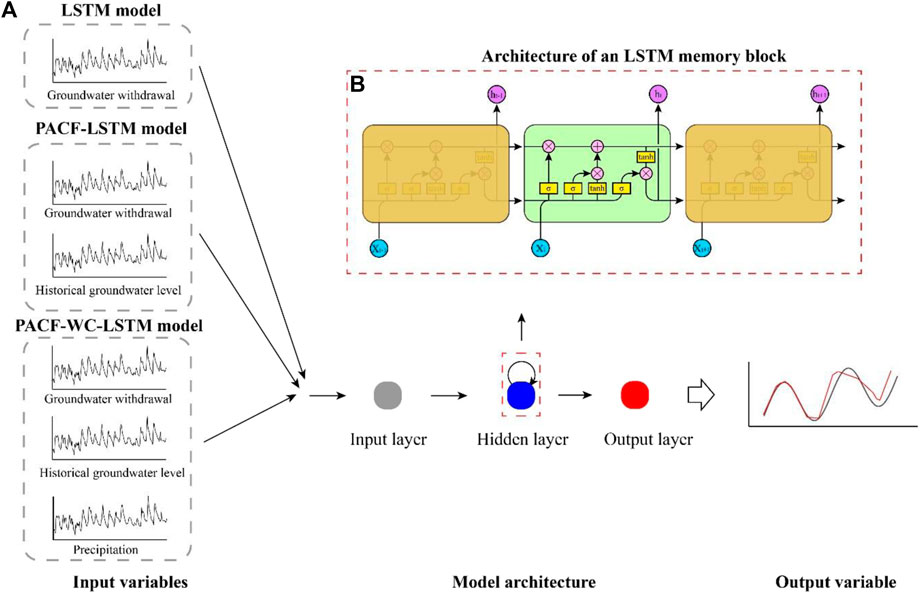
FIGURE 6. (A) A schematic flowchart for the LSTM model, PACF-LSTM model, and PACF-WC-LSTM model. (B) A schematic flowchart for an LSTM model Q14 modified from Yan et al. (2021).
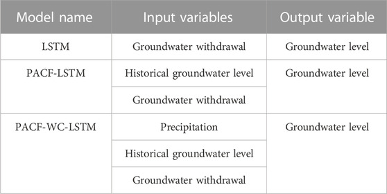
TABLE 1. The input and output variables of different models.
The validation and prediction results of the DG well, JF well, and KG well calculated by the LSTM model, PACF-LSTM model, and PACF-WC-LSTM model are shown in Figures 7–9, respectively. Their performance indexes are summarized in Table 2. Although the variation of groundwater level under the effect of groundwater exploitation could be fitted by the three different models, different error indicators indicated that the performance of the three models was different.
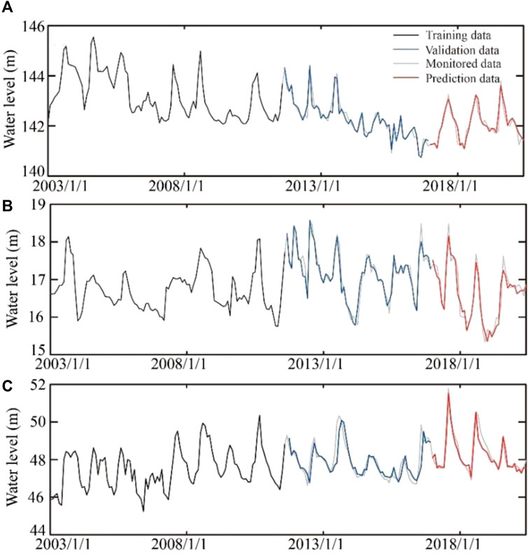
FIGURE 7. The training, validation, and prediction results of groundwater at (A) the DG well, (B) the JF well, and (C) the KG well by the LSTM method.
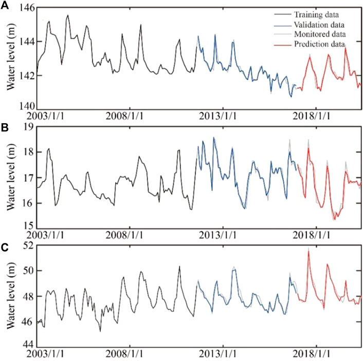
FIGURE 8. The training, validation, and prediction results of groundwater at (A) the DG well, (B) the JF well, and (C) the KG well by the PACF-LSTM method.
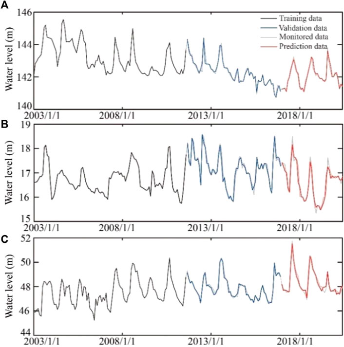
FIGURE 9. The training, validation, and prediction results of groundwater at (A) the DG well, (B) the JF well, and (C) the KG well by the PACF-WC-LSTM method.
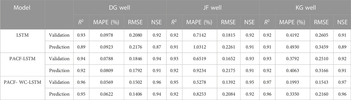
TABLE 2. The errors of three models in the validation and prediction stage in the DG well, the JF well, and the KG well.
NSE is the traditional efficiency indicator for evaluating the accuracy of hydrological models. For each monitoring well, the NSE value varied with different models. In the DG well, the NSE values of the validation and prediction stage in the LSTM model were 0.92 and 0.87, respectively, which were the smaller values in all three models. The smaller the NSE value is, the poorer the performance of the hydrological model. In comparison with the LSTM model, the PACF-LSTM model and PACF-WC-LSTM model increased the NSE values of the validation stage by 2% (from 0.92 to 0.94) and 4% (from 0.92 to 0.96), respectively (Table 3). For the prediction stage, the NSE values in the PACF-LSTM model and PACF-WC-LSTM model increased by 5% (from 0.87 to 0.91) and 8% (from 0.87 to 0.94), respectively. In addition, for the JF well, the change ratio of the NSE value was 1% and 3%, respectively, in the validation stage, and 0% and 1%, respectively, in the prediction stage. For the KG well, the change ratio of the NSE value was 1% and 7%, respectively, in the validation stage, and 2% and 8%, respectively, in the prediction stage. The results indicated that the quality of validation and prediction of the PACF-LSTM model and the PACF-WC-LSTM model were better than the LSTM model. Based on the error metric of NSE, the quality of the validation and prediction based on the PACF-WC-LSTM was the best in the three monitoring wells.
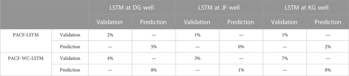
TABLE 3. The change ratio of NSE value in the three models at different monitoring wells.
RMSE is used to calculate the difference between the monitored value and the stimulated value. The smaller value of RMSE indicates that the model performance is perfect. Take the DG well as an example. For the LSTM model of the DG well, the RMSE values of the validation and prediction stages were 0.2080 and 0.2176, respectively. Compared with the LSTM model, the RMSE values of the PACF-LSTM and PACF-WC-LSTM models in the validation stage reduced by 11% (from 0.2080 to 0.1846) and 28% (from 0.2080 to 0.1502), respectively, and the values of the prediction stage reduced by 18% (from 0.2176 to 0.1792) and 35% (from 0.2176 to 0.1406), respectively (Table 4). For the validation stage in the other monitoring wells, the change ratio of RMSE value in the PACF-LSTM model was 9% and 4%, respectively, and the change ratio was 23% and 41%, respectively, in the PACF-WC-LSTM model. For the prediction stage in the other monitoring wells, the change ratio of RMSE value in the PACF-LSTM model was 4% and 8%, respectively, and it was 8% and 38%, respectively, in the PACF-WC-LSTM model. The change ratio of RMSE value also indicated that the prediction performance of PACF-WC-LSTM was the best in the three data-driven models.
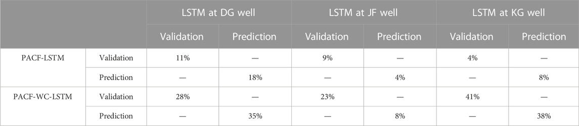
TABLE 4. The change ratio of RMSE value in the three models at different monitoring wells.
The MAPE value was introduced to evaluate the difference between the model prediction result and the monitored value as a percentage. For the DG well, the MAPE values in the validation stage and prediction stage of the LSTM model were 0.0978 and 0.0923, respectively. Those values in the PACF-LSTM model were reduced by 19% (from 0.0978 to 0.0788) and 12% (from 0.0923 to 0.0809), respectively. In the PACF-WC-LSTM model, those values were reduced by 42% (from 0.0978 to 0.0569) and 33% (from 0.0923 to 0.0622), respectively (Table 5). For the JF well, the change ratio of MAPE value in the validation stage was 9% for the PACF-LSTM model and 26% for the PACF-WC-LSTM model. Those values of the prediction stage were 10% and 20% for the PACF-LSTM model and PACF-WC-LSTM model, respectively. For the KG well, the change ratio of MAPE value in the PACF-LSTM model was 10% for the validation stage and 18% for the prediction stage. In the PACF-WC-LSTM model, those values were 52% and 32% in the validation stage and prediction stage, respectively.
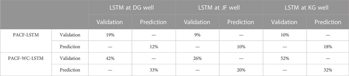
TABLE 5. The change ratio of MAPE value in the three models at different monitoring wells.
In order to analyze the prediction results by three models, the scatter plot of stimulated value and monitored value in the validation and prediction stage are displayed in Figures 10–12, respectively. The X-axis and Y-axis represent the monitored value and simulated value, respectively. If the model has perfect performance, the prediction results should be distributed over X = Y or evenly distributed on both sides of the line. The closer the distribution of scatter to the 1:1 line, the smaller the model error. R2 was introduced to evaluate the performance of different models. The results indicated that the performance of the PACF-WC-LSTM model was the best.
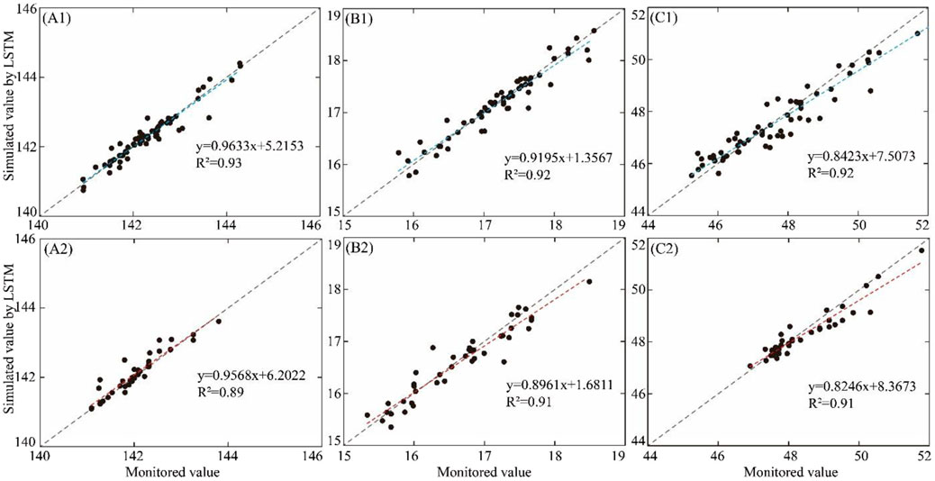
FIGURE 10. Scatter plot of the monitored value vs. the simulated value calculated by the LSTM method in the validation stage and prediction stage. (A1–C1) represent the validation stage of the LSTM model at (a) the DG well, (b) the JF well, and (c) the KG well, respectively. (A2–C2) represent the prediction stage of the LSTM model at (a) the DG well, (b) the JF well, and (c) the KG well, respectively. The blue and red dashed lines represent the trend lines of validation and prediction, respectively. Gray dotted lines represent a 1:1 line.
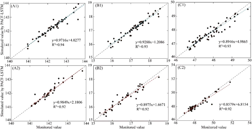
FIGURE 11. Scatter plot of the monitored value vs. the simulated value calculated by the PACF-LSTM method in the validation stage and prediction stage. (A1–C1) represent the validation stage of the PACF-LSTM model at (a) the DG well, (b) the JF well, and (c) the KG well, respectively. (A2–C2) represent the prediction stage of the PACF-LSTM model at (a) the DG well, (b) the JF well, and (c) the KG well, respectively. The blue and red dashed lines represent the trend lines of validation and prediction, respectively. Gray dotted lines represent a 1:1 line.
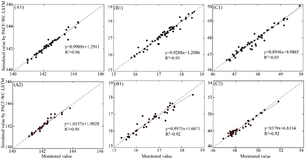
FIGURE 12. Scatter plot of the monitored value vs. the simulated value calculated by the PACF-WC-LSTM method in the validation stage and prediction stage. (A1–C1) represent the validation stage of the PACF-WC-LSTM model at (a) the DG well, (b) the JF well, and (c) the KG well, respectively. (A2–C2) represent the prediction stage of the PACF-WC-LSTM model at (a) the DG well, (b) the JF well, and (c) the KG well, respectively. The blue and red dashed lines represent the trend lines of validation and prediction, respectively. Gray dotted lines represent a 1:1 line.
Based on the abovementioned analysis, the quantitative evaluation metric for the three models indicates that the prediction performance of the PACF-WC-LSTM model is superior to those of the LSTM model and PACF-LSTM model.
For improving the accuracy of simulation and prediction of non-linear and non-stationary groundwater level change under the influence of groundwater exploitation in a coastal aquifer, we proposed a novel data-driven method called PACF-WC-LSTM, based on the combination of time series analysis and machine learning method. The prediction performance of PACF-WC-LSTM was compared with the LSTM model and the PACF-LSTM model by the error metric of R2, RMSE, NSE, and MAPE. These three models were applied to predict the change in groundwater level in three monitoring wells that were connected with different aquifer types. This study draws the following conclusions:
1) The partial autocorrelation function results indicate that a strong correlation relationship exists between the groundwater level data and the historical monitored data of groundwater level at three monitoring wells. The lag time is approximately 3 months for the groundwater level at the DG well, JF well, and KG well. The historical monitored data of groundwater level can be considered as the input variables for constructing the prediction model.
2) The continuous wavelet coherence results indicate that the groundwater level at three monitoring wells and precipitation are highly coherent within the band of about 1 year during the whole monitoring period. The dataset of precipitation can be considered as the input variables to construct a hydrological model.
3) Based on the results of the partial autocorrelation function and continuous wavelet coherence, three data-driven models, namely, the LSTM model, PACF-LSTM model, and PACF-WC-LSTM model, were constructed, and four error metrics, namely, R2, RMSE, NSE, and MAPE, were introduced to evaluate the model performance. The results indicate that the PACF-WC-LSTM model yields a better prediction performance than the LSTM model and the PACF-LSTM model, and can be used to predict the variation of groundwater level under the influence of groundwater exploitation in the coastal aquifer.
The raw data supporting the conclusion of this article will be made available by the authors, without undue reservation.
BG: Conceptualization, Data curation, Formal Analysis, Funding acquisition, Project administration, Writing–original draft. SZ: Conceptualization, Data curation, Formal Analysis, Methodology, Software, Writing–review and editing, Writing–original draft. KL: Conceptualization, Data curation, Funding acquisition, Methodology, Project administration, Writing–review and editing. PY: Conceptualization, Data curation, Formal Analysis, Funding acquisition, Project administration, Writing–review and editing. HX: Investigation, Visualization, Writing–review and editing. QF: Investigation, Visualization, Writing–review and editing. WZ: Funding acquisition, Project administration, Writing–review and editing. YZ: Investigation, Visualization, Writing–review and editing. WJ: Investigation, Visualization, Writing–review and editing.
The author(s) declare financial support was received for the research, authorship, and/or publication of this article. This study was funded by the China Geological Survey (DD20221677-2), CGS Research (JKYQN202307), and the Rizhao City Geological Survey (SDGP371100202102000475).
The authors declare that the research was conducted in the absence of any commercial or financial relationships that could be construed as a potential conflict of interest.
All claims expressed in this article are solely those of the authors and do not necessarily represent those of their affiliated organizations, or those of the publisher, the editors and the reviewers. Any product that may be evaluated in this article, or claim that may be made by its manufacturer, is not guaranteed or endorsed by the publisher.
Acworth, R. I., Halloran, L. J., Rau, G. C., Cuthbert, M. O., and Bernardi, T. L. (2016). An objective frequency domain method for quantifying confined aquifer compressible storage using Earth and atmospheric tides. Geophys. Res. Lett. 43 (22), 11671–11678. doi:10.1002/2016GL071328
An, L. X., Hao, Y. H., Yeh, T. C., Liu, Y., Liu, W. Q., and Zhang, B. J. (2020). Simulation of karst spring discharge using a combination of time-frequency analysis methods and long short-term memory neural networks. J. Hydrology 589, 125320. doi:10.1016/j.jhydrol.2020.125320
Barzegar, R., Fijani, E., Moghaddam, A. A., and Tziritis, E. (2017). Forecasting of groundwater level fluctuations using ensemble hybrid multi-wavelet neural network-based models. Sci. Total Environ. 599, 20–31. doi:10.1016/j.scitotenv.2017.04.189
Bredy, J., Gallichand, J., Celicourt, P., and Gumiere, S. J. (2020). Water table depth forecasting in cranberry fields using two decision-tree-modeling approaches. Agric. Water Manag. 233, 106090. doi:10.1016/j.agwat.2020.106090
Chen, C., He, W., Zhou, H., Xue, Y., and Zhu, M. D. (2020). A comparative study among machine learning and numerical models for simulating groundwater dynamics in the Heihe River Basin, northwestern China. Sci. Rep. 10 (1), 3904. doi:10.1038/s41598-020-60698-9
Chen, Z., Xu, H., Jiang, P., Yu, S. E., Lin, G., Bychkoy, I., et al. (2021). A transfer Learning-Based LSTM strategy for imputing Large-Scale consecutive missing data and its application in a water quality prediction system. J. Hydrology 602, 126573. doi:10.1016/j.jhydrol.2021.126573
Chien, S. H., Chi, W. C., and Ke, C. C. (2020). Precursory and coseismic groundwater temperature perturbation: an example from Taiwan. J. Hydrology 582, 124457. doi:10.1016/j.jhydrol.2019.124457
Daliakopoulos, I. N., Coulibaly, P., and Tsanis, I. K. (2005). Groundwater level forecasting using artificial neural networks. J. Hydrology 309 (1), 229–240. doi:10.1016/j.jhydrol.2004.12.001
Gao, X. H., Sato, K., and Horne, R. N. (2020). General solution for tidal behavior in confined and semiconfined aquifers considering skin and wellbore storage effects. Water Resour. Res. 56 (6). doi:10.1029/2020WR027195
Gu, X. F., Sun, H. G., Zhang, Y., Zhang, S. J., and Lu, C. P. (2022). Partial wavelet coherence to evaluate scale-dependent relationships between precipitation/surface water and groundwater levels in a groundwater system. Water Resour. Manag. 36 (7), 2509–2522. doi:10.1007/s11269-022-03157-6
Hakim, W. L., Nur, A. S., Rezaie, F., Panahi, M., Lee, C. W., and Lee, S. (2022). Convolutional neural network and long short-term memory algorithms for groundwater potential mapping in Anseong, South Korea. J. Hydrology Regional Stud. 39, 100990. doi:10.1016/j.ejrh.2022.100990
He, Y. Y., Zhou, Y., Wen, T., Zhang, S., Huang, F., Zou, X. Y., et al. (2022). A review of machine learning in geochemistry and cosmochemistry: method improvements and applications. Appl. Geochem. 140, 105273. doi:10.1016/j.apgeochem.2022.105273
Hikouei, I. S., Eshleman, K. N., Saharjo, B. H., Graham, L. B., Applegate, G., and Cohchrane, M. A. (2023). Using machine learning algorithms to predict groundwater levels in Indonesian tropical peatlands. Sci. Total Environ. 857, 159701. doi:10.1016/j.scitotenv.2022.159701
Hochreiter, S., and Schmidhuber, J. (1997). Long short-term memory. Neural Comput. 9 (8), 1735–1780. doi:10.1162/neco.1997.9.8.1735
Hosono, T., Shibata, Y. T., Wang, C. Y., Manga, M., Rahman, T. M. S., Shimada, J., et al. (2019). Coseismic groundwater drawdown along crustal ruptures during the 2016 Mw 7.0 kumamoto earthquake. Water Resour. Res. 55 (7), 5891–5903. doi:10.1029/2019WR024871
Hu, K. X., Awange, J. L., Kuhn, M., and Saleem, A. (2019). Spatio-temporal groundwater variations associated with climatic and anthropogenic impacts in South-West Western Australia. Sci. Total Environ. 696, 133599. doi:10.1016/j.scitotenv.2019.133599
Hussein, M. E. A., Odling, N. E., and Clark, R. A. (2013). Borehole water level response to barometric pressure as an indicator of aquifer vulnerability. Water Resour. Res. 49 (10), 7102–7119. doi:10.1002/2013WR014134
Kratzert, F., Klotz, D., Brenner, C., Schulz, K., and Herrnegger, M. (2018). Rainfall–runoff modelling using Long Short-Term Memory (LSTM) networks. Hydrology Earth Syst. Sci. 22 (11), 6005–6022. doi:10.5194/hess-22-6005-2018
Lee, E., and Kim, S. (2019). Wavelet analysis of soil moisture measurements for hillslope hydrological processes. J. Hydrology 575, 82–93. doi:10.1016/j.jhydrol.2019.05.023
Lee, S. H., Ha, K., Hamm, S. Y., and Ko, K. S. (2013). Groundwater responses to the 2011 tohoku earthquake on jeju island, korea. Hydrol. Process. 27 (8), 1147–1157. doi:10.1002/hyp.9287
Long, D., Yang, W. T., Scanlon, B. R., Zhao, J. S., Liu, D. G., Burek, P., et al. (2020). South-to-North Water Diversion stabilizing Beijing’s groundwater levels. Nat. Commun. 11 (1), 3665. doi:10.1038/s41467-020-17428-6
Mao, H. R., Wang, G. C., Liao, F., Shi, Z. M., Huang, X. J., Li, B., et al. (2022). Geochemical evolution of groundwater under the influence of human activities: a case study in the southwest of Poyang Lake Basin. Appl. Geochem. 140, 105299. doi:10.1016/j.apgeochem.2022.105299
Massei, N., Dupont, J. P., Mahler, B. J., Laignel, B., Fournier, M., Valdes, D., et al. (2006). Investigating transport properties and turbidity dynamics of a karst aquifer using correlation, spectral, and wavelet analyses. J. Hydrology 329 (1-2), 244–257. doi:10.1016/j.jhydrol.2006.02.021
Miyakoshi, A., Taniguchi, M., Ide, K., Kagabu, M., Hosono, T., and Shimada, J. (2020). Identification of changes in subsurface temperature and groundwater flow after the 2016 Kumamoto earthquake using long-term well temperature-depth profiles. J. Hydrology 582, 124530. doi:10.1016/j.jhydrol.2019.124530
Mohammed, H., Michel, H. T., and Seidu, R. (2022). Emulating process-based water quality modelling in water source reservoirs using machine learning. J. Hydrology 609, 127675. doi:10.1016/j.jhydrol.2022.127675
Nelson, D. B., Basler, D., and Kahmen, A. (2021). Precipitation isotope time series predictions from machine learning applied in Europe. Proc. Natl. Acad. Sci. 118 (26), e2024107118. doi:10.1073/pnas.2024107118
Nourani, V., Baghanam, A. H., Adamowski, J., and Kisi, O. (2014). Applications of hybrid wavelet-Artificial Intelligence models in hydrology: a review. J. Hydrology 514, 358–377. doi:10.1016/j.jhydrol.2014.03.057
Nourani, V., and Mousavi, S. (2016). Spatiotemporal groundwater level modeling using hybrid artificial intelligence-meshless method. J. Hydrology 536, 10–25. doi:10.1016/j.jhydrol.2016.02.030
Qu, S., Shi, Z. M., Wang, G. C., Xu, Q. Y., Han, J. Q., and Jiaqian, H. (2020). Using water-level fluctuations in response to Earth-tide and barometric-pressure changes to measure the in-situ hydrogeological properties of an overburden aquifer in a coalfield. Hydrogeology J. 28, 1465–1479. doi:10.1007/s10040-020-02134-w
Qu, S., Shi, Z. M., Wang, G. C., Zhang, H., Han, J. Q., Liu, T. X., et al. (2021). Detection of hydrological responses to longwall mining in an overburden aquifer. J. Hydrology 603, 126919. doi:10.1016/j.jhydrol.2021.126919
Rodrigues, E., Gomes, Á., Gaspar, A. R., and Henggeler, A. C. (2018). Estimation of renewable energy and built environment-related variables using neural networks – a review. Renew. Sustain. Energy Rev. 94, 959–988. doi:10.1016/j.rser.2018.05.060
Shi, Z. M., Zhang, S. C., Yan, R., and Wang, G. C. (2018). Fault zone permeability decrease following large earthquakes in a hydrothermal system. Geophys. Res. Lett. 45 (3), 1387–1394. doi:10.1002/2017GL075821
Sun, J. C., Hu, L. T., Li, D. D., Sun, K. N., and Yang, Z. Q. (2022). Data-driven models for accurate groundwater level prediction and their practical significance in groundwater management. J. Hydrology 608, 127630. doi:10.1016/j.jhydrol.2022.127630
Tawara, Y., Hosono, T., Fukuoka, Y., Yoshida, T., and Shimada, J. (2020). Quantitative assessment of the changes in regional water flow systems caused by the 2016 Kumamoto Earthquake using numerical modeling. J. Hydrology 583, 124559. doi:10.1016/j.jhydrol.2020.124559
Tinungki, G. M.Iop (2019). “The analysis of partial autocorrelation function in predicting maximum wind speed, 1st International Conference on Global Issue for Infrastructure, Environment and Socio-Economic Development,” in IOP Conference Series-Earth and Environmental Science, Bogar, West Java, 29 August 2019.
Tokunaga, T. (1999). Modeling of earthquake-induced hydrological changes and possible permeability enhancement due to the 17 January 1995 Kobe Earthquake, Japan. J. Hydrology 223 (3-4), 221–229. doi:10.1016/S0022-1694(99)00124-9
Vittecoq, B., Foritn, J., Maury, S., and Violette, S. (2020). Earthquakes and extreme rainfall induce long term permeability enhancement of volcanic island hydrogeological systems. Sci. Rep. 10 (1), 20231. doi:10.1038/s41598-020-76954-x
Vu, M. T., Jardani, A., Massei, N., and Fournier, M. (2021). Reconstruction of missing groundwater level data by using Long Short-Term Memory (LSTM) deep neural network. J. Hydrology 597, 125776. doi:10.1016/j.jhydrol.2020.125776
Wang, C. Y., Doan, M. L., Xue, L., and Barbour, A. J. (2018). Tidal response of groundwater in a leaky aquifer-application to Oklahoma. Water Resour. Res. 54 (10), 8019–8033. doi:10.1029/2018WR022793
Wang, C. Y., Liao, F., Wang, G. C., Qu, S., Mao, H. R., and Bai, Y. F. (2023). Hydrogeochemical evolution induced by long-term mining activities in a multi-aquifer system in the mining area. Sci. Total Environ. 854, 158806. doi:10.1016/j.scitotenv.2022.158806
Wang, C. Y., Wang, L. P., Manga, M., Wang, C. H., and Chen, C. H. (2013). Basin-scale transport of heat and fluid induced by earthquakes. Geophys. Res. Lett. 40 (15), 3893–3897. doi:10.1002/grl.50738
Wunsch, A., Liesch, T., and Broda, S. (2021). Groundwater level forecasting with artificial neural networks: a comparison of long short-term memory (LSTM), convolutional neural networks (CNNs), and non-linear autoregressive networks with exogenous input (NARX). Hydrol. Earth Syst. Sci. 25 (3), 1671–1687. doi:10.5194/hess-25-1671-2021
WWAP (2015). “Water for a sustainable world, no. 6.2015,” in The united nations world water development report (Paris, France: United Nations World Water Assessment Programme – UNESCO).
Xiao, Y., Hao, Q. C., Zhang, Y. H., Zhu, Y. C., Yin, S. Y., Qin, L. M., et al. (2022). Investigating sources, driving forces and potential health risks of nitrate and fluoride in groundwater of a typical alluvial fan plain. Sci. Total Environ. 802, 149909. doi:10.1016/j.scitotenv.2021.149909
Xiao, Y., Shao, J. L., Frape, S. K., Cui, Y. L., Dang, X. Y., Wang, S. B., et al. (2018). Groundwater origin, flow regime and geochemical evolution in arid endorheic watersheds: a case study from the Qaidam Basin, northwestern China. Hydrol. Earth Syst. Sci. 22 (8), 4381–4400. doi:10.5194/hess-22-4381-2018
Yan, R., Woith, H., Wang, R. J., and Wang, G. C. (2017). Decadal radon cycles in a hot spring. Sci. Rep. 7, 12120. doi:10.1038/s41598-017-12441-0
Yan, X., Shi, Z. M., Wang, G. C., Zhang, H., and Bi, E. P. (2021). Detection of possible hydrological precursor anomalies using long short-term memory: a case study of the 1996 Lijiang earthquake. J. Hydrology 599, 126369. doi:10.1016/j.jhydrol.2021.126369
Yan, X., Shi, Z. W., Zhou, P. P., Zhang, H., and Wang, G. C. (2020). Modeling earthquake-induced spring discharge and temperature changes in a fault zone hydrothermal system. J. Geophys. Res. Solid Earth 125 (7), e2020JB019344. doi:10.1029/2020JB019344
Yu, S. W., and Ma, J. W. (2021). Deep learning for geophysics: current and future trends. Rev. Geophys. 59 (3), e2021RG000742. doi:10.1029/2021RG000742
Yu, X., Wang, Y. H., Wu, L. F., Chen, G. H., and Qin, H. (2019). Comparison of support vector regression and extreme gradient boosting for decomposition-based data-driven 10-day streamflow forecasting. J. Hydrology 582, 124293. doi:10.1016/j.jhydrol.2019.124293
Zhang, H., Shi, Z. M., Wang, G. C., Yan, X., Liu, C. L., Sun, X. L., et al. (2021). Different sensitivities of earthquake-induced water level and hydrogeological property variations in two aquifer systems. Water Resour. Res. 57 (5), e2020WR028217. doi:10.1029/2020WR028217
Zhang, J. F., Zhu, Y., Zhang, X. P., Ye, M., and Yang, J. Z. (2018). Developing a Long Short-Term Memory (LSTM) based model for predicting water table depth in agricultural areas. J. Hydrology 561, 918–929. doi:10.1016/j.jhydrol.2018.04.065
Zhang, M. H., Li, X., and Wang, L. L. (2019). An adaptive outlier detection and processing approach towards time series sensor data. IEEE Access 7 (175192), 175192–175212. doi:10.1109/ACCESS.2019.2957602
Zhang, S. C., Shi, Z. M., Wang, G. C., Yan, R., and Zhang, Z. C. (2020). Groundwater radon precursor anomalies identification by decision tree method. Appl. Geochem. 121, 104696. doi:10.1016/j.apgeochem.2020.104696
Zhang, S. C., Shi, Z. M., Wang, G. C., Yan, R., and Zhang, Z. C. (2022a). Application of the extreme gradient boosting method to quantitatively analyze the mechanism of radon anomalous change in Banglazhang hot spring before the Lijiang Mw 7.0 earthquake. J. Hydrology 612, 128249. doi:10.1016/j.jhydrol.2022.128249
Keywords: long short term memory neural network, coastal groundwater levels, groundwater regime, groundwater withdrawal, machine learning
Citation: Guo B, Zhang S, Liu K, Yang P, Xing H, Feng Q, Zhu W, Zhang Y and Jia W (2023) Prediction of groundwater level under the influence of groundwater exploitation using a data-driven method with the combination of time series analysis and long short-term memory: a case study of a coastal aquifer in Rizhao City, Northern China. Front. Environ. Sci. 11:1253949. doi: 10.3389/fenvs.2023.1253949
Received: 07 July 2023; Accepted: 13 October 2023;
Published: 08 November 2023.
Edited by:
Ali Khenchaf, Laboratoire des Sciences et Techniques de l'Information de la Communication et de la Connaissance (LAB-STICC), FranceReviewed by:
George P. Karatzas, Technical University of Crete, GreeceCopyright © 2023 Guo, Zhang, Liu, Yang, Xing, Feng, Zhu, Zhang and Jia. This is an open-access article distributed under the terms of the Creative Commons Attribution License (CC BY). The use, distribution or reproduction in other forums is permitted, provided the original author(s) and the copyright owner(s) are credited and that the original publication in this journal is cited, in accordance with accepted academic practice. No use, distribution or reproduction is permitted which does not comply with these terms.
*Correspondence: Shouchuan Zhang, emhhbmdzY0BjYWdzLmFjLmNu; Kai Liu, YWNhbmNlckAxNjMuY29t
Disclaimer: All claims expressed in this article are solely those of the authors and do not necessarily represent those of their affiliated organizations, or those of the publisher, the editors and the reviewers. Any product that may be evaluated in this article or claim that may be made by its manufacturer is not guaranteed or endorsed by the publisher.
Research integrity at Frontiers
Learn more about the work of our research integrity team to safeguard the quality of each article we publish.