Enhancing oil-water flow simulation in shale reservoirs with fractal theory and meshless method

Introduction: Simulating oil and water flow in shale reservoirs is challenging due to heterogeneity caused by fractures. Conventional grid-based methods often have convergence issues. We propose a new approach using fractal theory and meshless methods to accurately model flow.

Methods: A mathematical model describing oil-water flow in fractured horizontal shale wells was developed. The meshless weighted least squares (MWLS) method was used to numerically solve the model. Modeling points were placed flexibly, informed by fractal theory.

Results: The MWLS solution aligned well with reference solutions but had enhanced flexibility. Comprehensive analysis showed the effects of modeling parameters like fracture properties on production.

Discussion: The proposed methodology enabled accurate prediction of shale oil production. Convergence was improved compared to grid-based methods. The flexible modeling approach can be tailored to specific reservoir conditions. Further work could expand the model complexity and types of reservoirs.

1 Introduction

Shale oil is an unconventional type of oil found in organic-rich black shale or nanoscale pores in shale. With vast reserves distributed worldwide, shale oil has become the most promising unconventional oil resource for development. However, shale oil reservoirs exhibit low matrix pore permeability and significant heterogeneity (Jia et al., 2019). Consequently, low fracture flowback rates often occur during the flowback process (Zhang et al., 2019), making accurate prediction of the oil and water flow in shale reservoirs crucial (Daneshy, 2004; Bertoncello et al., 2014; Su et al., 2016).

Due to the multi-scale nature and complex fluid distribution in shale oil reservoirs, traditional Darcy flow equations are insufficient for accurately depicting their flow characteristics. Researchers have adopted apparent porosity and permeability models to characterize the unique migration mechanisms in shales. These models can be grouped into three primary categories: Javadour models (based on fracture aperture) (Javadpour, 2009; Akkutlu et al., 2015; Singh and Javadpour, 2016), Civan models (based on the Knudsen number) (Civan, 2010; Wu et al., 2015; Song et al., 2016), Civan models (based on the Knudsen number) (Mason et al., 1983; Li et al., 2017; Zeng et al., 2017). In the study of oil behavior within nanopores, researchers have explored the use of organic/inorganic apparent porosity models. These models offer a valuable approach to characterize the oil state within nanopores, considering the influence of both organic and inorganic components. By incorporating the concept of apparent porosity, researchers aim to gain a deeper understanding of the distribution and behavior of oil within these nanoscale spaces (Sheng et al., 2019; Sheng et al., 2020). Furthermore, integrating the conventional dual-medium model with apparent permeability/porosity models has been found to provide a more accurate depiction of shale oil flow behavior (Sheng et al., 2018).

The heterogeneity of porosity and permeability in shale oil reservoirs poses challenges for numerical simulation, such as high computational costs and poor convergence (Li et al., 2023). Conventional grid-based finite difference methods are complex and not suitable for complex boundary conditions. Wei (Wei et al., 2021a) proposed a discontinuous discrete fracture model for coupled flow and geomechanics and used the finite element method to optimize the reservoir stress evolution (Shiming et al., 2022) and fracturing schemes for encrypted wells throughout the drilling-fracturing-producing wells (Wei et al., 2021b). Finite element meshes may experience severe distortion, requiring remeshing, which increases computational time and significantly affects accuracy. Describing complex geometric computational domains becomes cumbersome as further mesh refinement complicates preprocessing. Finite difference/volume methods are known for their accuracy; however, they have limitations when it comes to grid uniformity. High-precision difference schemes are often designed for regular Cartesian grids, which poses challenges when dealing with complex boundaries or reservoirs with intricate geological conditions. As a result, handling such situations becomes difficult using traditional finite difference/volume methods (Rao et al., 2020; Rao et al., 2022). Given the limitations of conventional numerical methods in simulating shale oil reservoirs, the meshless method emerges as a promising and efficient alternative. This method entails positioning points throughout the reservoir area to precisely delineate the intricate boundary of the shale oil reservoir. In this manner, the meshless technique develops a potent numerical model to emulate the movement of oil and water inside the shale oil deposit.

Introduced by Lucy in 1977, the Smoothed Particle Hydrodynamics (SPH) method is a mesh-free approach that has found success in addressing astrophysical problems. This method has been widely utilized in the simulation of various astrophysical phenomena, showcasing its effectiveness in capturing complex dynamics and fluid behavior without relying on traditional meshes (Lucy, 1977). Radial Basis Function (RBF) interpolation is an effective approach for generating smooth, continuous approximations of scattered data. In this technique, a collection of radial basis functions, such as Gaussian or multiquadric functions, are employed to estimate the solution at any point within the domain (Wright, 2003). The Element-free Galerkin (EFG) method is a meshless alternative to the Galerkin method, which is widely used in finite element analysis. Utilizing moving least squares (MLS) approximation, EFG constructs shape functions and integrates the PDE’s weak form throughout the domain. This method is applicable to both linear and nonlinear problems. (Belytschko et al., 1995). Li (Yu-kun, 2007) proposed the Mesh-Free Weighted Least Squares (MWLS) method, which has been recognized for its high accuracy and excellent stability, particularly in generating a symmetric coefficient matrix. Unlike the Galerkin method, the MWLS method does not require Gaussian integration, making it more efficient. Xu and Rao (Rao et al., 2021; Xu et al., 2021) applied the MWLS method to study shale gas water seepage problems, analyzing the influence of weight functions and nodes in the MWLS method. However, they did not specifically analyze the characteristics of shale oil.

In this paper, the concept of fractal permeability is introduced, and a numerical model is developed to simulate oil and water flow in a fractured horizontal well situated in a fractal shale oil reservoir. The Mesh-Free Weighted Least Squares (MWLS) method is employed to solve the problem. Additionally, a comparative analysis is conducted to evaluate the impacts of fracture distribution patterns, initial water saturation, and reservoir reconstruction degree on reservoir utilization scope and production performance. Through this analysis, insights are gained into the effective utilization and production performance of reservoirs under different conditions.

2 Equations for the meshless method in modeling oil-water flow in shale oil reservoirs

The meshless technique employs a collection of field nodes distributed across the computational domain’s boundary and body to delineate the boundary and the domain itself. Because these field nodes do not form any mesh, this technique can overcome the constraints of the finite difference approach, which necessitates a Cartesian mesh, as well as the finite element approach, which demands high-quality mesh production and remodeling.

The meshless method unfolds in three primary stages:

Step 1. Field Nodes in Meshless Techniques for Conveying Field Variable Values

Within the meshless approach, field variable values, encompassing unknown functions, are expressed by the nodal values assigned to field points. The precision of the computation is directly impacted by the concentration of these field points, which are typically spread evenly across the domain.

Step 2. Localized Approximation of Field Variables in Meshless Techniques

In meshless techniques, where a grid is not utilized, the field variables at a specific point x=(x₁,x₂) within the computational domain are approximated through interpolation using the field node values within the localized superconductive area centered around that point. This approach enables accurate estimation of field variable values at arbitrary locations, ensuring precise representation of the underlying physical phenomena.

$u\left(x\right)={\displaystyle \sum _{i=1}^n}{\varphi }_i\left(x\right)u_i={\mathrm{\Phi }}^T\left(x\right)U_s(1)$

Where, n denotes quantity of field nodes within a specific point’s local support domain x, u_i signifies the nodes’s value of the ith field node; U_s is The vector composed of the values at each field node; and φ_i(x) represents the shape function associated with the ith node in the support region of a given point x.

Step 3. Deriving Nodal Values of the Unknown Function in Meshless Techniques

Through the application of localized field variable approximations, the derivation of the shape function is done for the field points. The MLS approach is proficient in providing a shape function of high continuity across the overall problem sphere. Generally, when considering a global optimization problem, MLS simplifies the attainment of a globally optimal solution. Consequently, this paper leverages the MLS approach for the local approximation of field variables. In the scope of MLS, the approximation of the unknown function u(x) within x’s influence domain is performed.

$u^h\left(x\right)={\displaystyle \sum _{i=1}^m}{p}_i\left(x\right)a_i\left(x\right)=p^T\left(x\right)a\left(x\right)(2)$

Here, x represents the position in space of every node within the support region ${\mathrm{\Omega }}_x$ of the node under consideration, $p_i\left(x\right)$ operates as the principle basis function, m denotes the count of basis functions, and $a_i\left(x\right)$ denotes the vector of coefficients tied to the location coordinates. In the context of the MLS approximation $a_i\left(x\right)$, The decision on coefficients ensures the validity of the approximation function $u^h\left(x\right)$ optimally approximates the function to be solved in terms of the least squares within the ${\mathrm{\Omega }}_x$ of the node under review. These coefficients minimize the weighted norm in Eq. 3.

$J={\displaystyle \sum _{i=1}^n}\widehat{W}\left(x-x_i\right){\left[p^T\left(x_i\right)a\left(x\right)-u_i\right]}^2(3)$

Where n represents the quantity of nodes held in the support domain of the weight function $\widehat{\mathrm{W}}\left(x-x_i\right)\ne 0$, and u_i indicates the nodal parameter at the location x equals to xi.The necessary condition of making Eq. 3 minimum is

$\frac{\partial J}{\partial a}=0(4)$

That is,

$A\left(x\right)a\left(x\right)=B\left(x\right)U_s(5)$

In which,

$\begin{array}{l}A\left(x\right)={\displaystyle \sum _{i=1}^n}\widehat{W}\left(x-x_i\right)p\left(x_i\right)p^T\left(x_i\right)\\ B\left(x\right)=\left[\widehat{W}\left(x-x_1\right)p\left(x_1\right),\cdots ,\widehat{W}\left(x-x_n\right)p\left(x_n\right)\right]\end{array}(6)$

Then a(x) is:

$a\left(x\right)=A^{-1}\left(x\right)B\left(x\right)U_s(7)$

On substituting Eq. 6 into Eq. 2, it leads us to the conclusion that

$u^h\left(x\right)={\displaystyle \sum _{i=1}^n}{\varphi }_i\left(x\right)u_i={\mathrm{\Phi }}^T\left(x\right)U_s(8)$

In this context, Φ(x) represents a vector built from shape functions, determined by

${\mathrm{\Phi }}^T\left(x\right)=\left\{{\varphi }_1\left(x\right){\varphi }_2\left(x\right)\cdots {\varphi }_n\left(x\right)\right\}=p^T\left(x\right)A^{-1}\left(x\right)B\left(x\right)(9)$

So φ _i(x) is defined as

${\varphi }_i\left(x\right)={\displaystyle \sum _{j=1}^m}{p}_j\left(x\right){\left(A^{-1}\left(x\right)B\left(x\right)\right)}_{ji}=p^T\left(x\right){\left(A^{-1}B\right)}_i(10)$

It is important to note that while the shape function constructed on the basis of the point interpolation local approximation method possesses the Kronecker property, its usage of the local support domain fails to ensure compatibility throughout the entire domain.

2.1 Oil-water flow model of shale oil reservoir

In the geologic model for fractured horizontal wells within shale oil reservoirs, a binary porosity medium is proposed, comprised of two parts: the matrix substance and the fracture web. The matrix substance functions as the primary storage space, while the fracture network operates as the main channel for shale oil. Both oil and water have the capacity to move within the fractures, however, only oil has the ability to flow within the matrix. The dual-porosity model encompasses both the matrix and fracture systems: the former is the chief repository for shale oil, and the latter is the primary passage for it. Three basic assumptions are taken into account:

(1) The flow of oil-water takes place in the fracture system, while solely single-phase shale oil migrates towards fractures in the matrix, disregarding the flow within the matrix system;

(2) The influence of gravity and capillary forces is disregarded;

(3) Fluids exhibit minor compressibility, while rock material remains incompressible.

2.1.1 Flow model for the matrix system

Adhering to the principles of mass conservation and the Darcy flow equation, the oil flow equation within the matrix can be articulated as follows:

$-\frac{\sigma {\rho }_o{k}_{app}}{{\mu }_o}\left(p_m-p_f\right)=\frac{\partial \left({\varphi }_{app}{\rho }_o\right)}{\partial t}(11)$

where μ_o denotes the oil viscosity, in mPa·s; ρ_o denotes the oil density, in kg/m³; k_app represents the matrix apparent permeability, in mD; p_m refers to the matrix pressure, in MPa; p_f signifies the fracture network pressure, in MPa; φ_app stands for the matrix apparent porosity and t denotes time; $\sigma$ denotes the interfacial flow coefficient, 1/m².

The fracture system under scrutiny in this study is planar, possessing a uniform fracture spacing equal to 12/Lm, where Lm corresponds to the length of the matrix rock block’s side.

2.1.2 Flow model for the fracture system

Considering the principle of mass conservation along with Darcy’s law of flow, the equation for the water phase within a fracture system can be expressed as follows:

$\nabla \left[\frac{{\rho }_w{k}_f{k}_{rw}}{{\mu }_w}\nabla p_{wf}\right]+Q_m=\frac{\partial \left({\rho }_w{\varphi }_f{S}_w\right)}{\partial t}(12)$

The oil flow within the fracture is described as follows:

$\nabla \left[\frac{{\rho }_o{k}_f{k}_{ro}}{{\mu }_o}\nabla p_{of}\right]+Q_{\mathrm{m}}=\frac{\partial \left({\rho }_o{\varphi }_f{S}_o\right)}{\partial t}(13)$

where ρ_w signifies the water’s density, kg/m³; k_rw, k_ro denote the relative permeability of water and oil, respectively, mD; k_f represents the fracture’s permeability, mD;μ_w is the water’s viscosity, mPa•s; p_wf is the pressure within the water phase of the fracture, in MPa; φ_f is the fracture’s porosity; S_w and S_o indicate the water and oil saturations within the fracture, respectively; Q_mo is the mass flow rate, as shown in Eq. 14,

$Q_m={\rho }_i\frac{\sigma k_m}{{\mu }_i}\left(p_m-p_f\right)(14)$

Characteristics of the fracture system, like porosity and permeability, can be articulated as follows:

${\varphi }_f\left(x\right)={\varphi }_w{\left(\frac{x}{x_w}\right)}^{D_f-2-{\theta }_f}$

$k_f\left(x\right)=k_w{\left(\frac{x}{x_w}\right)}^{D_f-2-{\theta }_f}$

in this context, x denotes the distance from the origin, measured in meters (m), and x_w refers to the hydraulic fracture’s width, also measured in meters (m). The parameters ${\varphi }_w$ and kw represent the starting point’s porosity and permeability, respectively, in the matrix and fracture system medium, stated in millidarcies (mD). D_f is utilized to depict the fracture system medium’s geometric attributes, capturing the fractal fracture’s geometric nuances and intricacy. The anomaly diffusion index of the fracture system medium is conveyed by ${\varphi }_f$.

2.1.3 Supporting equations

For the purpose of this analysis, capillary forces are not considered. Therefore, the pressure of the oil within the fracture system equilibrates with the pressure of the water phase, resulting in the flow of only oil within the matrix system. Consequently, the pressures within the fracture and the matrix are denoted by P_f and P_m, respectively.

$S_o+S_w=1(15)$

$P_{wf}=P_{of}=P_f(16)$

Initial:

$p_i=p_f\left(x,y,z,0\right)=p_m\left(x,y,z,0\right)(17)$

2.2 Model solution

The meshless method, which is based on the weighted residual technique, utilizes the moving least squares (MLS) strategy to construct the approximation function. The governing equation is discretized using the least square method, resulting in the development of MWLS, a meshless technique. For a comprehensive understanding of the MWLS, please refer to the cited literature. (Yu-kun, 2007).

By reorganizing Eqs 11–13, we can derive the subsequent Eq. 18.

$\left\{\begin{array}{cc}\nabla \left({\lambda }_{fg}^t\nabla p_f^{t+1}\right)+\nabla \left({\lambda }_{fw}^t\nabla p_f^{t+1}\right)+q_{mg}^t-{\left({\varphi }_f{C}_{tf}\right)}^t\frac{p_f^{t+1}-p_f^t}{\partial t}=0& ①\\ \nabla \left({\lambda }_{fw}^t\nabla p_f^{t+1}\right)-{\varphi }_f^t\frac{S_w^{t+1}-S_w^t}{\partial t}=0& ②\\ \frac{\sigma k_m}{{\mu }_g}\left(p_m^{t+1}-p_f^{t+1}\right)+{\varphi }_m{C}_{tm}\frac{p_m^{t+1}-p_m^t}{\partial t}=0& ③\end{array}\right.(18)$

In the process of executing MWLS for inferential purposes, the problem domain, represented by Ω, and its boundary, denoted by Г, undergo discretization through the use of n points. The fracture system’s pressure and water saturation are then modeled by meshless approximate functions, established courtesy of MLS, which can be expressed following the template of Eq. 19.

$p_f\approx {\displaystyle \sum _{i=1}^n}{N}_i{P}_{fi}=N{d}_f(19)$

where $N=\left[N_1\left(x\right)N_2\left(x\right)N_3\left(x\right)\cdots N_n\left(x\right)\right]$ is a shape function, $d_f={\left[p_{f1}{p}_{f2}{p}_{f3}\cdots p_{fn}\right]}^T$.

By replacing Eq. 18-①) with Eq. 19 from above, the residual can be derived, as depicted in Eq. 20.

$\begin{array}{l}{R}_{p_f}=\nabla \left({\lambda }_{fw}^t\left(\nabla N{d}_f^{t+1}\right)\right)+\nabla \left({\lambda }_{fg}^t\nabla \left(N{d}_f^{t+1}\right)\right)+\frac{\sigma k_m}{{\mu }_g}\left(p_m^t-N{d}_f^{t+1}\right)\\ -{\left(\frac{{\varphi }_f{C}_{tf}}{\Delta t}\right)}^t\left(N{d}_f^{t+1}-N{d}_f^t\right)=0\end{array}(20)$

Thus, the computational scheme of MWLS for determining the pressure in the fracture system unfolds as follows:

$\begin{array}{l}{\mathrm{\Pi }}_{p_f}={\displaystyle \underset{\mathrm{\Omega }}{\int }}{\left(R_{p_f}\right)}^T{R}_{p_f}d\mathrm{\Omega }+{\displaystyle \underset{{\mathrm{\Gamma }}_1}{\int }}{\alpha }_1\left(N{d}_f^{t+1}-p_{fc}\right)\left(N{d}_f^{t+1}-p_{fc}\right)d\mathrm{\Gamma }\\ +{\displaystyle \underset{{\mathrm{\Gamma }}_2}{\int }}{\alpha }_2(\frac{\partial p_f^{t+1}}{\partial x})\left(\frac{\partial p_f^{t+1}}{\partial x}\right)d\mathrm{\Gamma }\end{array}(21)$

In Eq. 21, ${\alpha }_1$ and ${\alpha }_2$ symbolize the penalty functions for the boundary conditions. By identifying the least value of Eq. 21 and transposing it into a discrete format, we arrive at Eq. 22:

$\begin{array}{l}\delta {\mathrm{\Pi }}_{p_f}={\displaystyle \sum _{s=1}^n}\delta R_{p_f}{R}_{p_f}{|}_{x=x_s}+{\displaystyle \sum _{s=1}^{n_1}}{\alpha }_1\delta p_f^{t+1}{N}^T\left(N{d}_f^{t+1}-p_{fc}\right){|}_{x=x_s}\\ +{\displaystyle \sum _{s=1}^{n_2}}{\alpha }_2\delta p_f^{t+1}\nabla N^T\nabla N{|}_{x=x_s}=0\end{array}(22)$

By transforming Eq. 22 into matrix system and taking into account the freedom of $p_f^{t+1}$ , we derive Eq. 23.

$K_1{p}_f^{t+1}=F_1(23)$

Among them:

$\begin{array}{l}{K}_1={\displaystyle \sum _{s=1}^n}\left.\delta R_{p_f}{\left(\nabla {\lambda }_f^t\nabla \left(\nabla N\right)-\frac{\sigma k_m}{{\mu }_g}N-\left(\frac{{\varphi }_f{C}_{tf}}{\Delta t}\right)\right.}^{t}N\right)\\ +{\displaystyle \sum _{s=1}^{n_1}}{\alpha }_1{N}^{T}N+{\displaystyle \sum _{s=1}^{n_1}}{\alpha }_2\nabla N^T\nabla N\end{array}$

$F_1={\displaystyle \sum _{s=1}^n}\left.\delta R_{p_f}{\left(-\frac{\sigma k_m}{{\mu }_g}{p}_{gm}^t-\left(\frac{{\varphi }_f{C}_{tf}}{\Delta t}\right)\right.}^t{d}_f^t\right)+{\displaystyle \sum _{s=1}^{n_1}}{N}^T{p}_{fc}$

Eq. 24 provides the fracture’s pressure at the t+1 time step. This value is then utilized in Eq. (18-②) for substitution. Subsequently, the MLS method is employed to construct an approximate equation for the Sw in the fracture. Ultimately, Eq. 24 is derived:

$K_2{S}_w^{t+1}=F_2(24)$

Eq. 24 provides the fracture’s Sw at the next time step.

The variables and parameters involved are as follows:

$K_2={\displaystyle \sum _{s=1}^n}{N}^{T}N+{\displaystyle \sum _{s=1}^{n_1}}{\alpha }_1{N}^{T}N+{\displaystyle \sum _{s=1}^{n_2}}{\alpha }_2\nabla N^T\nabla N$

$F_2={\displaystyle \sum _{s=1}^n}{N}^T\left(e_{\mathrm{w}\mathrm{f}}^t+\frac{\Delta t}{{\varphi }_f}\left(\nabla {\lambda }_w^t\left(\nabla p_f^{t+1}\right)\right)\right)+{\displaystyle \sum _{s=1}^{n_1}}{\alpha }_1{N}^T{S}_{wfc}^t$

The matrix system’s pressure can be determined using a similar approach. By inserting the fracture system’s pressure at the next time step into formula (18-③), the final MWLS equation can be derived:

$K_3{p}_m^{t+1}=F_3(25)$

Eq. 25 provides the matrix’s pressure at the next time step.

The variables and parameters involved are as follows:

$K_3={\displaystyle \sum _{s=1}^n}\delta R_{p_m}\left(\frac{\sigma k_m}{{\mu }_g}N+\frac{{\varphi }_m{C}_{tm}N}{dt}\right)+{\displaystyle \sum _{s=1}^{n_1}}{\alpha }_1{N}^{T}N+{\displaystyle \sum _{s=1}^{n_2}}{\alpha }_2\nabla N^T\nabla N$

$F_3={\displaystyle \sum _{s=1}^n}\delta R_{p_m}\left(\frac{\sigma k_m}{{\mu }_g}{d}_f^{t+1}+\frac{{\varphi }_m{C}_{tm}}{dt}{p}_m^t\right)+{\displaystyle \sum _{s=1}^{n_1}}{\alpha }_1{N}^T{p}_{m{\mathrm{\Gamma }}_1}^t$

Where s represents the number of points used for calculations; Let n represent t the total number of points used for calculations within the neighborhood Ω, and let ni (i = 1,2) represent the total number of points used for calculations on boundary Γi.

3 Examining and confirming the accuracy of computational examples

3.1 Model validation

A field case was constructed to validate the model’s accuracy, considering the fractal features in a shale oil reservoir where the horizontal well is fractured. The reservoir area are 500 m × 400 m × 10m, with the model and layout depicted in Figure 1. The corresponding physical properties of the reservoir can be found in Table 1. Due to its superior continuity and higher computational accuracy, we used the Gaussian formulation as the weighting function in the grid-independent approach. The layout scheme used is 50 × 40, and a node spacing of 3 times (30 m) is used for the node influence domain.

FIGURE 1

FIGURE 1. Model figure.

TABLE 1

TABLE 1. Parameters of reservoir.

This study incorporated Table 1 data into the oil-water flow fractal shale reservoir model to obtain daily oil production variations. This paper set a result calculated using EDFM as the reference solution. The results were then compared to those of a reference solution, as shown in Figure 2. The proposed method closely matched the reference solution, demonstrating its reliability, accuracy, and high computational efficiency. Furthermore, Figure 3 presents the pressure distribution at different times, showing that the matrix pressure gradually decreases during production. Although there were some discrepancies between the reference solution and the MWLS results, these errors fall within acceptable bounds and can be attributed to inherent differences between the approaches.

FIGURE 2

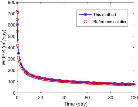
FIGURE 2. WOPR.

FIGURE 3

FIGURE 3. The Distribution of fracture pressure. (A) MWLS, 1 day; (B) Refence solution, 1 day; (C) MWLS, 50 day; (D) Refence solution, 50 day; (E) MWLS, 100 day; (F) Refence solution, 100 day.

3.2 Sensitivity analysis of nodal influence domain

After applying the theories and solutions mentioned earlier, a sensitivity analysis of the nodal influence domain is conducted to evaluate its impact on the accuracy of meshless method computations. The solution of the flow of oil and water in horizontally fractured wells. is used to verify the validity of the method. While the MWLS method is inherently precise, the accuracy of its results is also dependent on the process of choosing the nodal influence domain. The optimal parameter values vary depending on the specific problem at hand.

Consequently, the nodal influence domain was chosen to be 2, 3, 4, and 5 times the nodal spacing (10 m), with the initial water saturation is 0.25 while keeping other parameters constant. By doing so, the established mathematical model is further validated and analyzed to ensure its reliability and applicability in solving real-world problems associated with the flow of oil and water in horizontally fractured wells.

Figure 4 demonstrates the variation curves of daily oil and water production for different nodal influence domains. The calculated results demonstrate varying levels of consistency when the nodal influence domain is set at 2, 3, 4, and 5 times the nodal spacing. This suggests that the method is characterized by good stability and convergence in its calculations. This validates its effectiveness and robustness for simulating the flow of oil and water in horizontally fractured wells. Figure 5 shows the crack pressure distribution at 100 days for different nodal influence domains. The calculated crack pressure distributions do not differ significantly under different conditions. When the influence domain size is 5 times the nodal spacing, the pressure drop area is marginally larger than that for the influence domain size of 2, 3, and 4 times the nodal spacing. However, the overall difference is less than 2% because the area of pressure drop increases slightly with the size of the influence domain.

FIGURE 4

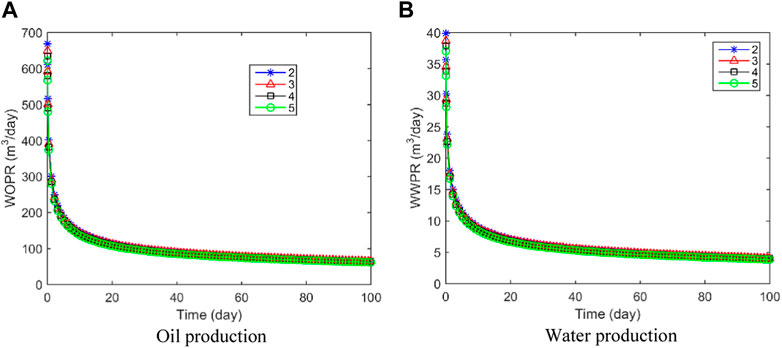
FIGURE 4. Comparsion of production. (A) Oil production; (B) Water production.

FIGURE 5

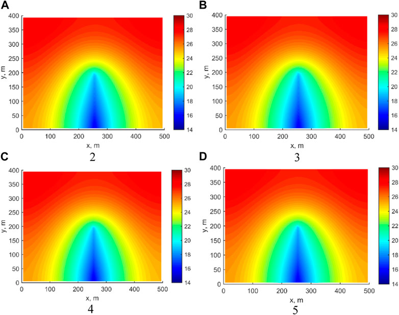
FIGURE 5. The distribution of frature pressure under different node influence domains. (A) 2; (B) 3; (C) 4; (D) 5.

3.3 Sensitivity analysis of initial Sw

The initial Sw level is a crucial factor affecting shale oil production. To investigate the impact of different initial Sw levels on reservoir recovery and fractured well production while keeping other parameters constant, data from Table 1 were utilized. The initial Sw values were set at 0.35, 0.45, 0.55, and 0.65. Figure 6 illustrates the pressure in the reservoir for different initial levels of Sw after 100 days of production. It is evident that an increase in the initial Sw level leads to a reduction in the pressure difference between the matrix and fracture in the reservoir. This underscores the importance of accurately modeling and understanding initial Sw when simulating and predicting shale oil production. At an initial Sw of 0.35, the matrix pressure in the upper part of the model is about 30 MPa at 100 days, while at this value of 0.65, the matrix pressure in the upper part of the model is only about 26 MPa.

FIGURE 6

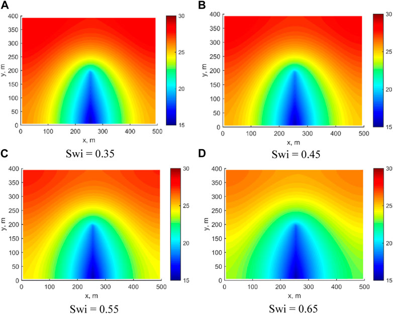
FIGURE 6. Pressure distribution under different initial Sw. (A) Swi = 0.35; (B) Swi = 0.45; (C) Swi = 0.55; (D) Swi = 0.65.

In Figure 7, the Sw distribution in the reservoir at 100 days are shown for different initial Sw levels. When the initial Sw is set at 0.35, the Sw at the fracture increases slightly to 0.3506 after 100 days. However, as the initial Sw level increases, the Sw at the fracture decreases after 100 days. This phenomenon is mainly due to the increase in Sw, which results in a significant rise in water flow capacity. Accurately modeling and predicting the behavior of oil-water flow in shale reservoirs requires an understanding of the relationship between initial Sw and its impact on fracture Sw over time.

FIGURE 7

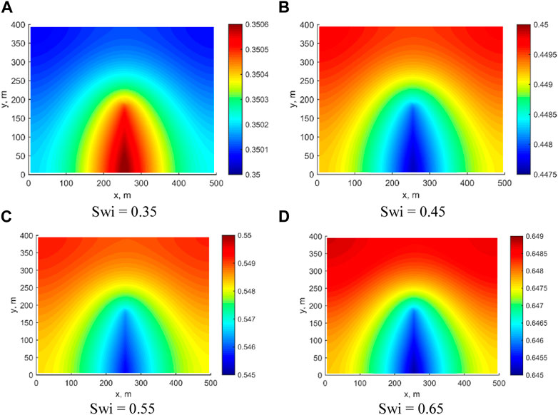
FIGURE 7. Fracture Sw distribution under different initial Sw. (A) Swi = 0.35; (B) Swi = 0.45; (C) Swi = 0.55; (D) Swi = 0.65.

In Figure 8, the fluid production under different initial Sw conditions is displayed. As the initial Sw increases, there is less free oil stored in the fractures and reservoirs. Consequently, the initial oil production is significantly reduced when the initial Sw is higher. Moreover, higher Sw reduces the relative permeability of the oil phase, hindering oil flow within the reservoir. Thus, larger initial Sw levels result in lower daily oil production and higher daily water production. For instance, when the initial Sw is set at 0.65, the initial daily well water production rate can reach 1024 m³/day. Understanding these relationships is crucial for optimizing reservoir management and production strategies.

FIGURE 8

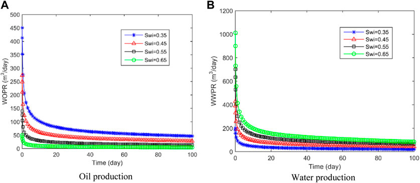
FIGURE 8. Production of different initial water saturation conditions. (A) Oil production; (B) Water production.

3.4 Sensitivity analysis of fracture half-lengths

We investigate the effects of different fracture half-lengths on the proposed model by setting the values to 100 m, 150 m, 200 m, 250 m, and 300 m, while keeping other parameters unchanged. This analysis helps to understand how variations in fracture half-length and SRV influence the production performance and recovery efficiency in shale oil reservoirs.

Figure 9 displays the pressure distribution field for different fracture half-lengths at 100 days. Increasing the fracture half-length results in a more rapid and extensive drop in matrix pressure. For instance, with a fracture half-length of 100 m, the matrix pressure in the upper part of the reservoir was maintained at 30 MPa, while at a fracture half-length of 300 m, it decreased to 27 MPa.

FIGURE 9

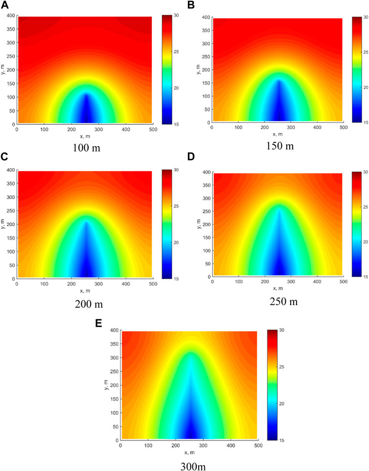
FIGURE 9. Pressure distribution of different fracture half-lengths. (A) 100 m; (B) 150 m; (C) 200 m; (D) 250 m; (E) 300 m.

Figure 10 depicts the comparison curves of daily and cumulative oil production for various fracture half-lengths. Daily oil production rises with an increase in the fracture half-length, as shown in Figure 10A. Figure 10B indicates a positive correlation between cumulative oil production and fracture half-length, mainly due to the larger stimulated reservoir volume and pressure ripple area as the fracture half-length increases. Despite this, the incremental gain in cumulative oil production diminishes as the fracture half-length increases. For example, when the fracture half-length is 100 m, the cumulative oil production for 100 days is 8075 m³. When the fracture half-length is extended to 150 m, the cumulative oil production increases by 1556 m³ to reach 9631 m³. However, when the fracture half-length is increased from 250 m to 300 m, the increase in cumulative oil production is only 602 m³.

FIGURE 10

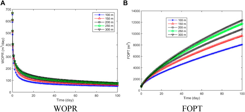
FIGURE 10. WOPR and FOPT of different fracture half-lengths. (A) WOPR; (B) FOPT.

3.5 Effects of fracture numbers

There are multiple factors affecting oil well productivity, among which the number of fractures is one of the key factors. The optimization of fracture numbers is also an important aspect of design of hydraulic fractures for horizontal wells. By fixing fracture half-length at 200 m, setting the initial Sw at 0.65, we change the number of fractures to 2, 3, 4, and 5, keeping other parameters consistent with the previous example.

The pressure distribution at 100 days for different fracture numbers is displayed in Figure 11. The relationship between the number of fractures and the pressure in the reservoir is evident, with an increase in fractures leading to a more rapid decline in pressure and a larger affected area. For example, when there are 2 fractures, the matrix pressure at the upper end of the reservoir can still be maintained at 25 MPa. However, when there are 5 fractures, the matrix pressure at the upper end of the reservoir is only 20 MPa. Figure 12 presents the changes in production capacity under different fracture numbers. Figures 12A, B display the wopr and wwpr curves, respectively, indicating that as the number of fractures increases, the corresponding WOPR and WWPR also increase. Figure 12C shows the FOPT curve, which is also shows a positive correlation with the number of fractures, but the rate of increase is diminishing. Increasing the number of fractures from 2 to 4 results in a 1.28-fold increase in cumulative oil production. However, increasing the number of fractures from 4 to 5 only leads to a 1.05-fold increase in cumulative oil production.

FIGURE 11

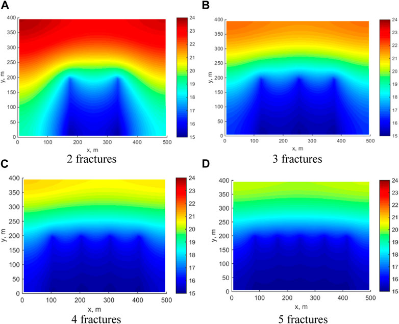
FIGURE 11. Pressure distribution at 100 days. (A) 2 fractures; (B) 23 fractures; (C) 4 fractures; (D) 5 fractures.

FIGURE 12

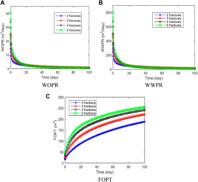
FIGURE 12. Production capacity analysis. (A) WOPR; (B) WWPR; (C) FOPT.

4 Conclusion

1) A mathematical model for oil-water fractal diffusion in fractured horizontal wells considering fracture network heterogeneity was developed and numerically solved using the MWLS method. Field example validation confirmed the model’s accuracy.

2) The impact of nodal domains in MWLS method was explored. The method shows robust stability. With an expanding nodal influence domain, the calculated results converge towards true values.

3) Employing the model, we examined the effects of initial Sw and reservoir modification on reservoir utilization and production. Increasing initial Sw increases oil flow resistance, hence reducing oil production. During reservoir modification, expanding fracture half-length and count enhances oil production, but with diminishing growth rate.

Data availability statement

The raw data supporting the conclusion of this article will be made available by the authors, without undue reservation.

Author contributions

WL conceptualization, methodology, software, writing—original draft, formal analysis GZ supervision, Project administration. All authors contributed to the article and approved the submitted version.

Conflict of interest

The authors declare that the research was conducted in the absence of any commercial or financial relationships that could be construed as a potential conflict of interest.

Publisher’s note

All claims expressed in this article are solely those of the authors and do not necessarily represent those of their affiliated organizations, or those of the publisher, the editors and the reviewers. Any product that may be evaluated in this article, or claim that may be made by its manufacturer, is not guaranteed or endorsed by the publisher.

References

Akkutlu, I. Y., Efendiev, Y., and Savatorova, V. J. T. i. P. M. (2015). Multi-scale asymptotic analysis of gas transport in shale matrix. Transp. Porous Media 107, 235–260. doi:10.1007/s11242-014-0435-z

CrossRef Full Text | Google Scholar

Belytschko, T., Lu, Y. Y., Gu, L., and Tabbara, M. (1995). Element-free Galerkin methods for static and dynamic fracture. Int. J. Solids Struct. 32, 2547–2570. doi:10.1016/0020-7683(94)00282-2

CrossRef Full Text | Google Scholar

Bertoncello, A., Wallace, J., Blyton, C., Honarpour, M., and Kabir, C. (2014). Imbibition and water blockage in unconventional reservoirs: well-management implications during flowback and early production. SPE Res. Eval. & Eng. 17, 497–506. doi:10.2118/167698-PA

CrossRef Full Text | Google Scholar

Civan, F. (2010). Effective correlation of apparent gas permeability in tight porous media. Transp. Porous Media 82, 375–384. doi:10.1007/s11242-009-9432-z

CrossRef Full Text | Google Scholar

Daneshy, A. (2004). “Analysis of off-balance fracture extension and fall-off pressures,” in SPE International Symposium and Exhibition on Formation Damage Control, Lafayette, Louisiana, February 2004. doi:10.2118/86471-MS

CrossRef Full Text | Google Scholar

Javadpour, F. J. J. o. C. P. T. (2009). Nanopores and apparent permeability of gas flow in mudrocks (shales and siltstone). J. Can. Pet. Technol. 48, 16–21. doi:10.2118/09-08-16-da

CrossRef Full Text | Google Scholar

Jia, B., Tsau, J. S., and Barati, R. (2019). A review of the current progress of CO2 injection EOR and carbon storage in shale oil reservoirs. Fuel 236, 404–427. doi:10.1016/j.fuel.2018.08.103

CrossRef Full Text | Google Scholar

Li, Z., Lei, Z., Shen, W., Martyushev, D. A., and Hu, X. (2023). A comprehensive review of the oil flow mechanism and numerical simulations in shale oil reservoirs. Energies 16, 3516. doi:10.3390/en16083516

CrossRef Full Text | Google Scholar

Li, Z., Zhang, X., and Liu, Y. J. G. (2017). Pore-scale simulation of gas diffusion in unsaturated soil aggregates: Accuracy of the dusty-gas model and the impact of saturation. Geoderma 303, 196–203. doi:10.1016/j.geoderma.2017.05.008

CrossRef Full Text | Google Scholar

Lucy, L. B. (1977). A numerical approach to the testing of the fission hypothesis. Astronomical J. 82, 1013–1024. doi:10.1086/112164

CrossRef Full Text | Google Scholar

Mason, E. A., Ea, M., and Ap, M.(1983). Gas transportin porous media: The dusty-gas model.

Google Scholar

Rao, X., Cheng, L., Cao, R., Jia, P., Liu, H., and Du, X. (2020). A modified projection-based embedded discrete fracture model (pEDFM) for practical and accurate numerical simulation of fractured reservoir. J. Petroleum Sci. Eng. 187, 106852. doi:10.1016/j.petrol.2019.106852

CrossRef Full Text | Google Scholar

Rao, X., Xin, L., He, Y., Fang, X., Gong, R., Wang, F., et al. (2022). Numerical simulation of two-phase heat and mass transfer in fractured reservoirs based on projection-based embedded discrete fracture model (pEDFM). J. Petroleum Sci. Eng. 208, 109323. doi:10.1016/j.petrol.2021.109323

CrossRef Full Text | Google Scholar

Rao, X., Zhan, W., Zhao, H., Xu, Y., Liu, D., Dai, W., et al. (2021). Application of the least-square meshless method to gas-water flow simulation of complex-shape shale gas reservoirs. Eng. Analysis Bound. Elem. 129, 39–54. doi:10.1016/j.enganabound.2021.04.018

CrossRef Full Text | Google Scholar

Sheng, G., Javadpour, F., and Su, Y. (2018). Effect of microscale compressibility on apparent porosity and permeability in shale gas reservoirs. Int. J. Heat Mass Transf. 120, 56–65. doi:10.1016/j.ijheatmasstransfer.2017.12.014

CrossRef Full Text | Google Scholar

Sheng, G., Javadpour, F., and Su, Y. J. F. (2019). Dynamic porosity and apparent permeability in porous organic matter of shale gas reservoirs. Fuel 251, 341–351. doi:10.1016/j.fuel.2019.04.044

CrossRef Full Text | Google Scholar

Sheng, G., Zhao, H., Su, Y., Javadpour, F., Wang, C., Zhou, Y., et al. (2020). An analytical model to couple gas storage and transport capacity in organic matter with noncircular pores. Fuel 268, 117288. doi:10.1016/j.fuel.2020.117288

CrossRef Full Text | Google Scholar

Shiming, W., Yan, J., Jiawei, K., Yang, X., and Botao, L. (2022). Reservoir stress evolution and fracture optimization of infill wells during the drilling-fracturing-production process. Acta Pet. Sin. 43, 1305. doi:10.7623/syxb202209009

CrossRef Full Text | Google Scholar

Singh, H., and Javadpour, F. J. F. (2016). Langmuir slip-Langmuir sorption permeability model of shale. Fuel 164, 28–37. doi:10.1016/j.fuel.2015.09.073

CrossRef Full Text | Google Scholar

Song, W., Yao, J., Li, Y., Sun, H., Zhang, L., Yang, Y., et al. (2016). Apparent gas permeability in an organic-rich shale reservoir. Fuel 181, 973–984. doi:10.1016/j.fuel.2016.05.011

CrossRef Full Text | Google Scholar

Su, Y., Sheng, G., Wang, W., Zhang, Q., Lu, M., and Ren, L. J. F. (2016). A mixed-fractal flow model for stimulated fractured vertical wells in tight oil reservoirs. Fractals 24, 1650006. doi:10.1142/s0218348x16500067

CrossRef Full Text | Google Scholar

Wei, S., Jin, Y., Liu, X., and Xia, Y. (2021b). “The optimization of infill well fracturing using an integrated numerical simulation method of fracturing and production processes,” in Abu Dhabi International Petroleum Exhibition & Conference, Abu Dhabi, UAE, November 2021. doi:10.2118/207978-MS

CrossRef Full Text | Google Scholar

Wei, S., Kao, J., Jin, Y., Shi, C., and Liu, S. (2021a). A discontinuous discrete fracture model for coupled flow and geomechanics based on FEM. J. Petroleum Sci. Eng. 204, 108677. doi:10.1016/j.petrol.2021.108677

CrossRef Full Text | Google Scholar

Wright, G. B. (2003). Radial basis function interpolation: Numerical and analytical developments. Colorado: University of Colorado at Boulder.

Google Scholar

Wu, K., Li, X., Wang, C., Chen, Z., and Yu, W. J. A. J. (2015). A model for gas transport in microfractures of shale and tight gas reservoirs. AIChE J. 61, 2079–2088. doi:10.1002/aic.14791

CrossRef Full Text | Google Scholar

Xu, Y., Sheng, G., Zhao, H., Hui, Y., Zhou, Y., Ma, J., et al. (2021). A new approach for gas-water flow simulation in multi-fractured horizontal wells of shale gas reservoirs. J. Petroleum Sci. Eng. 199, 108292. doi:10.1016/j.petrol.2020.108292

CrossRef Full Text | Google Scholar

Yu-kun, L. (2007). Meshless numerical well-test on complex fault-block reservoir.

Google Scholar

Zeng, Y., Ning, Z., Lei, Y., Huang, L., Lv, C., and Hou, Y. (2017). “Analytical model for shale gas transportation from matrix to fracture network,” in SPE Europec featured at 79th EAGE Conference and Exhibition, Paris, France, June 2017. doi:10.2118/185794-MS

CrossRef Full Text | Google Scholar

Zhang, G., Chen, R., Hu, G., Huang, W., zhang, X., and liu, H. (2019). Low-cost drilling Technology for horizontal wells with atmospheric shale gas in the outer margin of sichuan basin. IOP Conf. Ser. Earth Environ. Sci. 295, 042098. doi:10.1088/1755-1315/295/4/042098

CrossRef Full Text | Google Scholar