 Ayşe Çay Atalay
 Yusuf Akan
94% of researchers rate our articles as excellent or good
Learn more about the work of our research integrity team to safeguard the quality of each article we publish.
Find out more
ORIGINAL RESEARCH article
Front. Environ. Sci., 13 October 2023
Sec. Environmental Economics and Management
Volume 11 - 2023 | https://doi.org/10.3389/fenvs.2023.1243278
This article is part of the Research TopicDeterminants of Sustainable Development from a Global PerspectiveView all 5 articles
The present study aims to examine the effect of the geographical location relationship between economic growth and environmental pollution. For this purpose, the spatial relationship between the variable CO2 emission and the variables energy consumption (ENC), real GDP per capita (GDP), urbanization rate (URB), and trade liberalization (DAE) was investigated by using the data of 37 OECD countries for the period of 1990–2015. The geographical location relationship was determined by using LISA (Local Indicators of Spatial Association) analysis, which is one of the spatial autocorrelation analysis methods. Spatial distribution maps were prepared. Considering the years determined according to Moran I index results, a gradually increasing positive autocorrelation was found for CO2 and ENC variables and a low increasing positive correlation for DAE and GDP variables. For the variable URB, a low increasing positive autocorrelation was found for the year 1990 and a high increasing positive autocorrelation for the year 2015. Then, using the LISA clustering maps, the relationships between the countries were clustered as low, high, and non-related. As a result of this study, given the spatial analysis results, the effect of energy consumption on the carbon emission was found to be positive in general. Increases in trade liberalization increased carbon emissions in some countries and decreased it in some others. On the other hand, increases in the urbanization rate decreased carbon emissions in some countries and had a positive effect in some others. The trade openness index was found to have a generally negative effect on the carbon emission. Within the scope of this study, Spatial Regression Analysis was conducted separately for the years 1990 and 2015. In this analysis, CO2 is the dependent variable, whereas ENC, GDP, URB, and DAE are independent variables. Given the results of spatial regression analysis, it was found that ENC, GDP, and DAE variables have a positive relationship with the CO2 variable. It was determined that there was no significant relationship between URB and CO2. Considering the results achieved, it could be possible to observe the increasing and decreasing effects of variables, which were examined here, on the CO2 emissions.
• Spatial analysis was performed to determine the effect of the location between economic growth and environmental pollution
• In the spatial analysis, the zones were created on a country basis. In addition, the LISA (Local Indicators of Spatial Association) analysis method was used to determine autocorrelation.
• Variables determined as green economy indicators, data of OECD countries were obtained from the World Development Indicators database.
• In the study, spatial regression analysis was performed to create a statistical model with the variables affecting CO2 emission.
• As a result of the study, an increase in CO2 emissions was observed in most of the countries.
The green economy is based on the rational use of environmental resources. It promotes the development of technology having less harm to the environment, a lower carbon footprint, and more social inclusion. (Velame and Teixeira, 2017; Xing et al., 2023). Organizations such as the United Nations Environment Program (UNEP, 2011) define the green economy as a path to sustainability. Furthermore, this term is also used in addressing the finance and climate change crisis. The OECD defines green growth as fostering economic growth and development, while ensuring that natural assets continue to provide the resources and environmental services on which our wellbeing relies (Capasso et al., 2019). At this point, as an approach that has internalized the social justice and where the economic system propagates to the entire base, the green economy distinguishes itself from the current economic systems with its perspective that has been shaped in parallel with the demands of environmentalists and green politicians (Şahin, 2015)1.
In the industrialization policies that continued until the 1960s, it was thought that physical conditions would allow all countries to industrialize and grow their industries continuously. While environmental problems started to pose serious threats at the end of the 1960s, it was realized in the 1970s that the main reason for this was the existing understanding of development. It became evident that the concept of development and the level of production and consumption increasing with the growing population contradict the idea of sustainability (Zhao et al., 2020). At this point, the general belief was that nature does not get polluted and, even if it gets polluted, it would clean itself. In fact, this misconception was partly because, in Arthur Burn’s words, ‘the depreciation of the environment was not deducted when calculating the national income’. Rapid urbanization and increasing consumption of natural resources, caused by rapid population growth, brought environmental problems to the fore almost everywhere in the world, regardless of the level of development of countries, and it became a threat to all humanity (Gwartney et al., 2010).
Considering the period between 2005 and 2015, as stated by the Sendai Framework Document for Disaster Risk Reduction declared by the United Nations, more than 700,000 individuals lost their lives, more than 1.4 million individuals were injured, and approximately 23 million individuals became homeless. In total, 1.5 billion people have been affected by various disasters. Women, children, and disadvantaged groups suffered more. The total economic loss was more than $1.3 trillion. The Earth has warmed by 1°C in the last century and experts predict that it could handle a warming by 1.5°C at maximum (Akay, 2019). Considering all these developments, if the world, in all areas and as a whole, fails to realize the green growth approach against the classical growth approach, then these results can be considered as signals of greater disasters.
In the year 2011, OECD initiated the Green Growth Strategy. Within this context, the transition of countries to the green economy, which supports economic growth efforts by paying attention to ecological balance while using the natural resources and preserving biological diversity in the way preventing ecological degradation. Green preservation and green standards should not prevent the efforts aiming to resolve the current socioeconomic problems but encourage the green economic development. Particular attention was paid to the economic modernization that defines traditional environmental protection policies as the environmentally friendly management of environmental resources contributing to social and environmental development. It was emphasized that the common characteristic of current economic and social models and green economic models is sustainability (Jezierska-Thole et al., 2022; Xing et al., 2023).
In this study, it was aimed to explain the effects of the amount of pollution caused by the gradual increase in the levels of industrialization and welfare worldwide on the environment also through the relationship with geographical location. During the research, the starting point was if the spatial effect would be included in the factors influencing the pollution for the OECD countries. The novelty of the present study is the use of a large geographical area, where the spatial proximity and distance relationship is tested, to monitor the effects of variables influencing the level of pollution. In this study, the geographical distribution of OECD countries examined offered an advantage to more clearly observe the effects of spatial proximity and distance relationship. Considering the studies in the literature, the effects of geographical location on the variables have been widely discussed, especially in recent years. The effect of geographical location was tested by using multiple countries and multiple variables in this study.
The main reason for the development of spatial econometrics and spatial statistics is the need for measuring how data are affected by their location. Waldo Tobler explained the basic law of geography in 1970 as follows; “Everything is related to other things, but things that are close together are more related than things that are far from each other.” From this point of view, similar values of a variable are observed in close proximity to each other and the spatial clustering occurs. The assumption of independence of observations is not valid in the presence of spatial clusters (Anselin, 1996). In the present study, energy consumption, per capita real gross domestic product (GDP), urbanization rate, and trade liberalization data of countries were used, their effects on CO2 emissions were also tested with regression analysis, and the findings were interpreted. The spatial analysis method, which has been widely used in social sciences in recent years, was tested on OECD countries in this study. From this aspect, besides contributing to the literature in terms of comparing with frequently used methods, it will also provide a different perspective for future studies.
The importance of the studies examining the environment gradually increases. The results achieved from these studies are very important for the measures to be taken for the environment because our Earth has limited time to spend testing some decisions with test-fail approach. From this perspective, the need to implement empirically verified results with ecological measures without delay highlights the importance and necessity of developing such studies.
Nowadays, environmental pollution is the biggest problem that the world is facing, and the habitats around the world are directly or indirectly affected by this problem. The most important aspect of growth is its contribution to the general welfare of society. Economic growth is necessary because it allows society to consume more goods and services. The provision of larger quantities of goods and services (health, education, etc.) leads to a real improvement in living standards. However, accelerated economic growth may lead to the depletion of natural resources and the worsening of environmental pollution problems (Azam, 2019; Anser et al., 2021; Huang et al., 2022). While establishing the model (1.1) used here, the variables to be used were determined by reviewing the studies in the literature. Moreover, the characteristics of OECD countries were also considered while selecting the variables. This study covers a large area and it aims to develop a different perspective by visually illustrating the comparison between multiple countries.
Undoubtedly, one of the main determinants of the growth and development of countries is the per capita GDP (gross domestic product). The fact that OECD countries, which the present study was carried out on, consist of high- or upper-medium-income countries strengthens the correlation between income and growth. Growth is a factor that increases the CO2 emission. Thus, it was aimed to observe the effect of GDP on pollution by adding this variable into the model (Shang et al., 2023). Many studies have been carried out to determine the relationship between growth and environmental pollution by making use of different methods. The most important effect of the increase in the pollution rate on the environment is the increase in the increasing greenhouse gas emissions. Carbon dioxide (CO2) is the main source of greenhouse gas. The causal relationship between greenhouse gases produced by human activities and global warming was proven in the fifth assessment report of the United Nations Intergovernmental Panel on Climate Change (IPCC) in 2014 (Shao et al., 2019; Huang et al., 2022). Gross domestic product is the most widely used measure of the size of an economy (Ponce and Khan, 2021; Maroufi and Hajilary, 2022). The origin of research on GDP and environmental pollution is defined under the Environmental Kuznets Curve (EKC) hypothesis, which is based on the Kuznets curve developed by Kuznets (Kuznets, 1955). However, a lot of empirical research has been done to investigate the negative effects of growth on the environment.
In recent studies, the relationship between the energy consumption variable and pollution is one of the frequently researched subjects. Any use of energy is necessary to sustain many economic activities and produce goods and services. Therefore, while the increase in production increases the need for energy, it also leads to an increase in CO2 emissions and environmental pollution (Çamkaya et al., 2022). Countries need energy to continue many economic activities, produce goods and services, and maintain social and economic developments. Moreover, it is considered as a fundamental factor in reducing the poverty and increasing the welfare level and living standards (Alkan and Albayrak, 2020). ENC variable was added to the model since the fact that OECD countries include both developing and developed countries would cause these countries to have different energy consumption and pollution levels. In many studies, it was tried to measure the amount of pollution created by using different types of energy, such as fossil fuel use such as oil and coal and CO2 emissions (Acar and Lindmark, 2017), electricity consumption and CO2 emissions (Asumadu-Sarkodie and Owusu, 2016; Asumadu-Sarkodie and Owusu, 2017), and the relationship between renewable energy sources and CO2 emissions (Hasnisah et al., 2019; Kirikkaleli and Adebayo, 2021).
From a general perspective, urbanization describes the migration from rural areas to cities. Urbanization has numerous and versatile effects on CO2 emissions (Niu and Lekse, 2017). Considering the structures of OECD countries, developed and developing countries differ in terms of urbanization rate. URB variable was added to the model in order to observe the differences between the countries in terms of CO2 emissions. The energy-growth-emission relationship is related to the urbanization and environment. Studies showed that urbanization can increase both income and energy use, and such an increase is evident at all stages of urbanization progression (Khan et al., 2019; Zhou, 2019; Guo et al., 2023). Many factors such as household size, changing industrial structure, increase in the number of new residences and new public facilities, and city size distribution increase the level of pollution (Abbasi et al., 2020). Many studies have been carried out on a local and national basis and they showed that rapid industrialization and urbanization caused an increase in CO2 emissions. CO2 emissions, whether overall or per capita, are affected by regional characteristics (Khoshnevis and Golestani, 2019).
The relationship between trade and the environment is one of the important research topics. Since the 1990s, the positive and negative effects of trade openness on the environment have been the subject of the Environmental Kuznets Curve (EKC), Pollution Paradise, and Race to the Bottom hypotheses (Fan et al., 2019). Some of the studies revealed that the increase in foreign trade increased CO2 emissions (Ansari et al., 2019; Liu et al., 2019; Nurgazina et al., 2021). Some other studies revealed that foreign trade has no effect on CO2 emissions or it changes depending on the export rate and time (Mutascu, 2018; Salahuddin et al., 2018; Lv and Xu, 2019; Iqbal et al., 2021). Adding DAE into the model, it was aimed to test the effects of trade relationships between countries (neighbors or not) on CO2 emissions according to both approaches by considering the geographical locations of OECD countries.
Spatial analysis methods have been frequently used in recent years. Thus, the classical methods used to explain real-life relationships have been replaced by spatial models that take location labels into account while explaining the relationships between variables (Başar, 2009). Using the spatial analysis method, the trends of the factors affecting CO2 emissions in the form of increase, decrease, and remaining constant has been observed in many studies (Panayotou, 2016; Chen et al., 2019; Yang et al., 2019; Jezierska-Thöle et al., 2022). This aspect of the study is expected to contribute to the literature.
In this study, the variables that analyze the effect of economic growth on environmental degradation and are selected in parallel with the studies in the literature were first analyzed with the EKC method. Then, for the spatial analysis, the GDP2 variable was removed from the model developed and the model was established as follows.
In Eq. 1, CO2 refers to carbon dioxide emissions (metric ton/person), ENC to energy use (oil equivalent kg/person), GDP per capita to real gross domestic product (US$ in 2010 constant prices). DAE to the trade openness index (share of exports and imports in the gross domestic product), and URB to urbanization rate (share of the urban population in the total population).
The data used in the study cover the years 1990–2015, and in model no 1, the coefficient β0 is the constant term and it represents other variables that are not included in the model. The coefficient β1 (ENC) shows the change in carbon dioxide emissions versus a 1% change in energy consumption. The coefficient β2 (GDP), however, shows the change in carbon dioxide emissions versus a 1% change in gross domestic product and the variable β3 represents the openness index (DAE) and represents the 1% impact on carbon dioxide emissions. Finally, the variable β4 (URB) shows the effect of a 1% change in the urbanization rate on carbon dioxide emissions. The data used in the analysis were obtained from the World Bank (World Development Indicators-WDI) database.
In this research, firstly, a spatial model of the variables was created with the explanatory spatial data analysis method. Regional decompositions were determined by map distributions and Moran scatter diagrams. The parameters of the model were estimated by the least squares method. Spatial dependency tests were conducted to determine whether the model contains spatial dependence. After determining the type of spatial dependence, the spatial model was created by including the dependency in the model. The study was completed by using the maximum likelihood method for the parameters of the spatial regression model. In the study, the trends of increase, decrease, and remaining constant in all variables for the beginning and ending years are also presented visually with thematic maps. In addition, by applying regression analysis to the model, it was determined that the error variances were equal and normal distribution so that the model could be used.
Moran scatter diagrams were prepared to observe the spatial interaction of the map distributions and the variables in which regional differences are shown visually. The graph is scattered across four regions by the Moran I values of the countries. The maps by the regions of these countries in the graph were obtained by making use of LISA analysis. Spatial regression analysis was performed with the data set method determined in the last stage. In Spatial Regression, the decision-making process was followed step by step. The results were interpreted according to the significance levels of ***0.01, **0.05, *0.10.
In the regression model, some tests are conducted to detect the presence of spatial dependence. These.
• Lagrange multiplier test,
• Moran I test,
• Resistive (Robuts) Lagrange multiplier tests
• Combined LM test
Before the spatial effects are predicted, it should be tested if the spatial dependence will be added into the model as a spatial delay or as a spatial error. Therefore, Anselin proposed the Lagrange Multiplier (LM) test, which was developed by Anselin in 1988 and determines the structure of the dependency for the spatial error self-relation in the presence of a lagged dependent variable (Anselin, 1988; Yılgör, 2019).
where, tr (trace) represents the sum of the diagonal elements of the matrix.
Contrary to Moran I test approach, it is based on the maximum likelihood method. The hypotheses for the
The LM lag test, another spatial dependency test related to the LM method, is formulated as follows.
The hypotheses for the
While the H0 hypothesis states that the spatial autoregressive parameter is not significant, the H1 hypothesis states that this parameter is significant (Anselin and Rey, 1991).
The most common method used to test spatial autocorrelation is Moran’s I statistic applied to regression residuals. The statistics is expressed as follows.
Here, n represents the number of observations, W represents the spatial weight matrix,
It is the standardization factor that shows the sum of the non-zero weights of the spatial weight matrix. In the weight matrix standardized according to the rows, this total number of units gives n. Since
The null hypothesis of this test clearly states that there is no spatial dependence, whereas the alternative hypothesis does not express a sharp type of dependence. Since the spatial correlation structure under the alternative hypothesis is not clear, this test only investigates spatial sequential dependence and does not provide information about the type of addiction (Anselin and Rey, 1991; Anselin, 1998; Aral, 2016).
They created the Robust determination test, which was developed by Bera and Yoon in 1993 and using the asymptotic distributions of the LM tests. This test contains differences in the covariance and mean of the LM statistic. Based on this study, Anselin et al. developed Robust statistics in 1996 (Anselin et al., 1996; Aral, 2016).
Robuts transformation tests are used to determine which model originates from the spatial dependence. In the presence of a spatial lag-dependent variable, it tests the spatial error dependence, and in the presence of a spatial error dependence, it tests the spatial lag dependency.
Under the assumption of λ ≠ 0, 0, the hypothesis H0: ρ = 0, Under the assumption of ρ ≠ 0, it tests the H0: λ = 0 hypothesis (Zeren, 2011).
Here
In case of
Here
If
The joint LM test tests the co-significance of the spatial delay and spatial error models. The joint LM test is expressed as follows.
The joint LM test statistic yields the sum of the LM statistics obtained from the
This test has an asymptotic χ^2 distribution with a degree of freedom of 2 (Anselin et al., 1996).
In the estimation of spatial regression models, the most widely used method is the maximum likelihood (ML) method. This method was first introduced by Keith Ord in the year 1975. In the ML approach, the probability calculation of the common distribution of the observations is maximized according to a set of parameters. The ML estimation has the desired asymptotic properties (efficiency, consistency, and asymptotic normality, etc.).
The logarithmic likelihood function for the spatial delay model is as follows (Anselin, 1988).
To estimate the parameters with the maximum likelihood method, the model should be maximized with respect to σ2 and β. However, the parameters of the logarithmic likelihood function are not linear. Anselin proposed substituting some of the parameters in the original likelihood function in order to reduce the number of unknowns in the problem. For this purpose, the likelihood function is reduced to a condensed likelihood function through the estimates obtained for σ2 and β. The parameters of the spatial autoregressive model and the estimation steps of β by Anselin in 1988 are as follows (Zeren, 2011).
• In the classical regression model,
•
• The residues
•
• With the help of
By applying these steps, the coefficients for the lag model are obtained (Anselin, 1988; LeSage and Pace, 1999).
The steps in estimating the parameters of the spatial error model developed by (Ord, 1975) are as the following.
• Residues are obtained from the
•
The
• The variables
• By regressing
•
• These steps are repeated until convergence is achieved (Ord, 1975; Zeren, 2011)
In the model developed by Anselin in 2005, the steps and operation are followed as schematically illustrated in Figure 1. The first step is to conduct a classical regression analysis. Classical regression model results are examined and LM statistics are examined considering if there is a dependency or not. If LMλ and LMρ are statistically insignificant, then it is concluded that there is no spatial dependence. In this case, the spatial error model and the spatial delay model will not be valid. Thus, it is decided to use the results obtained from the classical regression model.
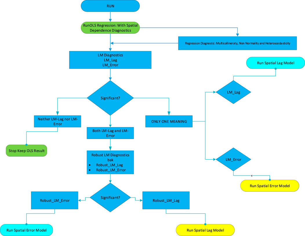
FIGURE 1. Classical regression model estimation process. Source: Anselin and Rey, 2014.
If the LMλ test, which examines only the spatial error dependence of the LM statistics, is statistically significant, the study is continued with the spatial error model. If the LMρ test, which examines the dependence of the spatial delay, is statistically significant, then the study continues with the spatial delay model.
If both LMλ and LMρ tests are statistically significant, then RLMλ and RLMρ tests are conducted in order to determine where the spatial dependence originates from. If the RLMλ test in which the error dependence is tested is significant, then the spatial error model is used. If the RLMρ test in which the delay dependence is examined is significant, then the spatial delay model is used.
Map plays an important role in descriptive spatial data analysis. Maps allow for visualizing the pattern of the spatial distribution. In applications, quartile maps that divide the dataset into four equal parts are used in general (Fıscher Manfred and Jinfeng, 2011). At this point, for the variables used in the study, maps were created using CO2 emissions, ENC, GDP, URB, and DAE data for the years 1990 and 2015 to observe the increase, decrease, or stability in the variables.
It can be seen in 1990–2015 CO2 change maps (Figure 2) that, in the CO2 emission map, the countries with the highest CO2 emissions are shown in the darkest colors. As the colors become lighter, the CO2 emission rates decrease. Comparing the data of 1990 and 2015, CO2 emissions increased in Japan, Korea, New Zealand, and Norway. On the other hand, CO2 emissions decreased in Denmark, France, Germany, and Hungary. No change in CO2 emissions was observed in Australia, Austria, Belgium, Canada, Chile, Colombia, Czech Republic, Estonia, Finland, Greece, Iceland, Ireland, Israel, Italy, Latvia, Lithuania, Luxembourg, Mexico City, Netherlands, Poland, Portugal, Slovakia, Slovenia, Spain, Sweden, Switzerland, Turkey, the United Kingdom, and the United States.
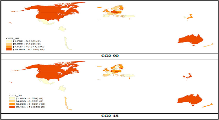
FIGURE 2. Comparative distribution maps of CO2 for 1990–2015.
As can be seen in 1990–2015 ENC rates maps (Figures 3, 4), considering the energy usage rates and comparing the years 1990 and 2015, ENC rates increased in Austria, Israel, Japan, Korea, Slovenia, and Spain. It decreased in Estonia, Hungary, Latvia, Lithuania, Slovakia, Switzerland, United Kingdom. There was no change in Australia, Belgium, Canada, Chile, Colombia, Czech Republic, Denmark, Finland, France, Germany, Greece, Iceland, Ireland, Italy, Luxembourg, Mexico, Netherlands, New Zealand, Norway, Poland, Portugal, Sweden, Turkey, and the United States.
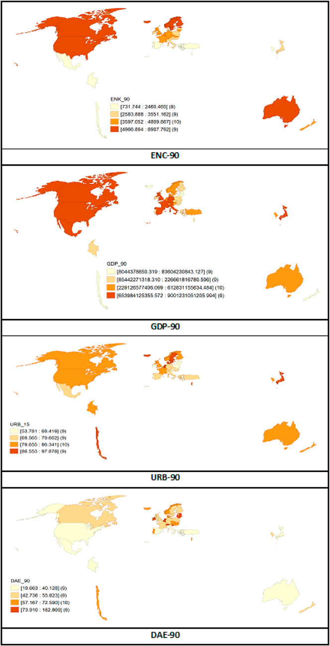
FIGURE 3. Comparative distribution maps of variables for 1990.
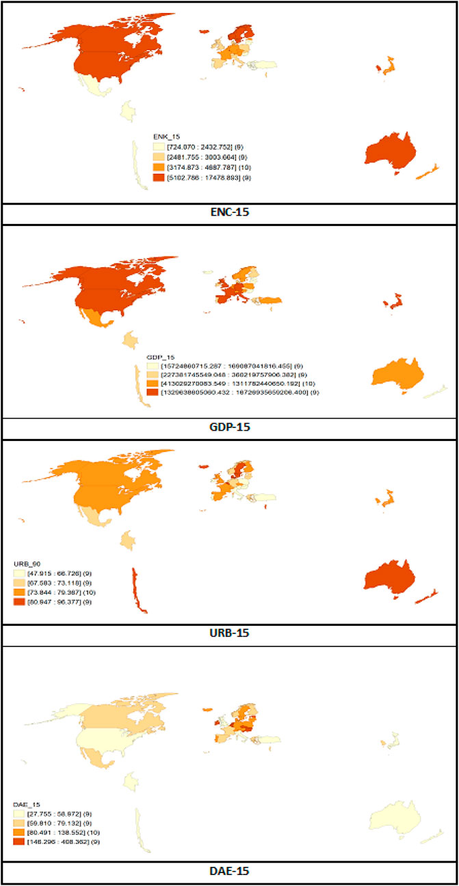
FIGURE 4. Comparative distribution maps of variables for 2015.
It can be seen in 1990–2015 GDP rates maps (Figures 3, 4) that, examining the GDP indicators of OECD countries, GDP decreased in Denmark, Hungary, and Mexico in 1990 and 2015. It increased in Chile, Korea, and Poland. No change was observed in Austria, Australia, Belgium, Canada, Colombia, Czech Republic, Estonia, Finland, France, Germany, Greece, Iceland, Ireland, Israel, Italy, Japan, Latvia, Lithuania, Luxembourg, Netherlands, New Zealand, Norway, Portugal, Slovakia, Slovenia, Spain, Sweden, Switzerland, Turkey, the United Kingdom, and the United States.
As can be understood from 1990–2015 URB rates maps (Figures 3, 4), given the data on urbanization rates of OECD countries, urbanization rates decreased in Australia, Czech Republic, Estonia, Latvia, Lithuania, New Zealand, Spain, and Switzerland in 1990 and 2015. It increased in Colombia, Hungary, Italy, Japan, the Netherlands, Norway, and Turkey. No change was observed in Austria, Belgium, Canada, Chile, Denmark, Finland, France, Germany, Greece, Iceland, Ireland, Israel, Korea, Luxembourg, Mexico, Poland, Portugal, Slovakia, Slovenia, Sweden, the United Kingdom, and the United States.
It can be seen in 1990–2015 openness index rates (DAE) maps (Figures 3, 4) that, given the openness index DAE indicators, DAE decreased in Chile, Germany, Israel, Latvia, Lithuania, New Zealand, Norway, Switzerland, and the United Kingdom in 1990 and 2015. It increased in the Czech Republic, Greece, Hungary, Mexico, Poland, Spain, and Sweden, whereas no change was observed in Austria, Australia, Belgium, Canada, Colombia, Denmark, Estonia, Finland, France, Iceland, Ireland, Italy, Japan, Korea, Luxembourg, Netherlands, Portugal, Slovakia, Slovenia, Turkey, and the United States.
The spatial interaction of the variables, regional differences of which are shown visually with the map distributions, are examined by making use of Moran scatter diagrams. Moran I value in the scatter diagram refers to the slope of the regression curve between the values of the relevant variable and the values obtained by multiplying by the spatial weight matrix of the variable (Anselin, 1996). In spatial autocorrelation, global effects originate from regional variations, whereas local effects originate from the spatial dependence between neighboring regions (Bivand and Wong, 2018).
LISA analysis, which is a local indicator of spatial relationship, is used to examine whether the observation values show regionally significant spatial clustering or segregation. The Moran scatter diagram consists of four main regions, and the countries are scattered over the four regions of the graph by their Moran I values. These countries can be mapped to the regions in the chart by using LISA analysis. In the LISA analysis, countries at the 1% significance level can be grouped into four clusters, which are HH, LH, LL, and HL. Moran scatter diagrams and LISA clustering maps for the years 1990 and 2015 of green economy indicators of OECD countries are given below.
Figure 5 shows that, given the CO2 emission data, Moran I value was determined to be 0.121 in 1990 and 0.187 in 2015. These values show that there is a positive autocorrelation between the CO2 emission values of the countries. It was found that autocorrelation increased in 2015.
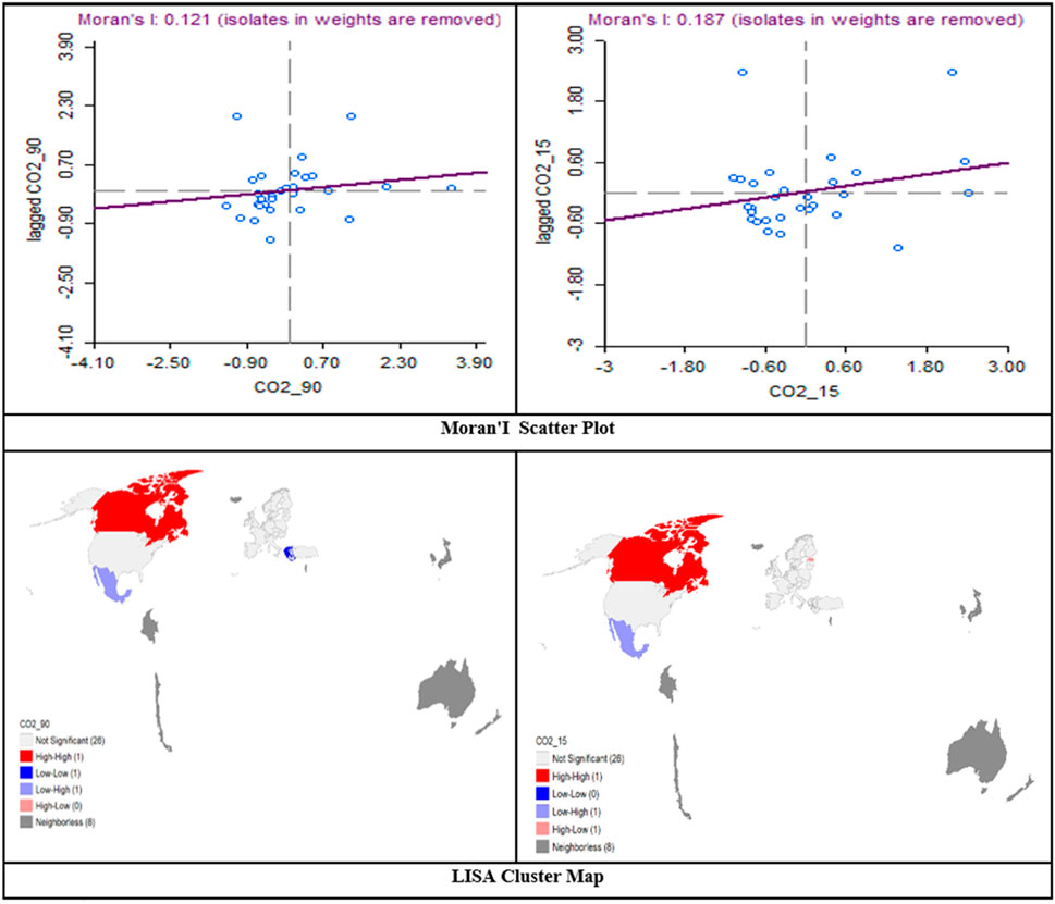
FIGURE 5. Moran Scatter Diagrams of CO2 data of OECD countries and LISA clustering maps for the period of 1990–2015.
LISA maps show that, considering the 1990s CO2 emissions, Canada was clustered in HH, Mexico in LH, and Greece in LL. Other countries were not clustered into any of these four significance levels.
Considering 2015s CO2 emissions, Canada is clustered in HH, Estonia in HL, and Mexico in LH. While Estonia could not be included in any cluster at the significance level in 1990, it was clustered in HL at the significance level of 1% in 2015. Mexico was clustered in LH in 1990 and LH in 2015. While Canada was clustered in HH in 1990, it was clustered in HH in 2015.
Figure 6 shows that Moran I value of the ENC ratio variable was determined to be 0.313 in 1990 and 0.486 in 2015. These values indicate that there is a positive autocorrelation between the values of the countries. It was found that autocorrelation increased in 2015.
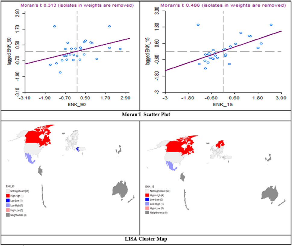
FIGURE 6. Moran Scatter Diagrams of ENC data of OECD countries and LISA clustering maps for the period of 1990–2015.
LISA clustering maps were created using ENK data of 1990 and 2015 for OECD countries. In 1990, Canada was clustered in HH, Mexico in LH, and Greece in LL at the significance level of 1%. In 2015, Canada, Finland, Norway, and Sweden were clustered in HH and Mexico in LH. While Finland, Norway, and Sweden were not included in any cluster at the significance level of 1% in 1990, they were clustered in the HH cluster in 2015. While Greece was clustered in LL in 1990, it was not included in any cluster in 2015.
Figure 7 shows that Moran I value of the GDP variable was calculated to be 0.012 in 1990 and 0.035 in 2015. Considering the GDP variable, it was determined that there was positive autocorrelation between countries. LISA maps show that Canada was clustered in HH, Denmark and Mexico in LH, and Estonia and Latvia in LL in 1990–2015 at a significance level of 1%.
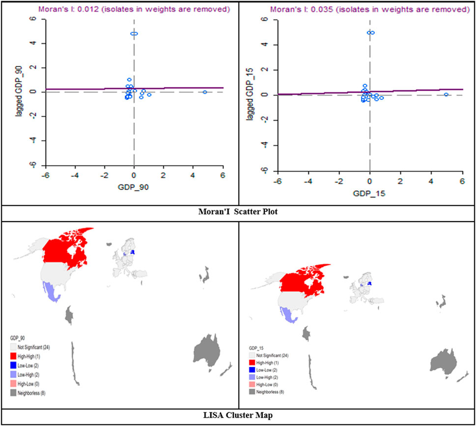
FIGURE 7. Moran Scatter Diagrams of GDP data of OECD countries and LISA clustering maps for the period of 1990–2015.
Figure 8 shows that, while the Moran I value of the urbanization rate variable was 0.115 in 1990, this rate increased to 0.474 in 2015. It was determined that there was positive autocorrelation between countries regarding the URB variable.
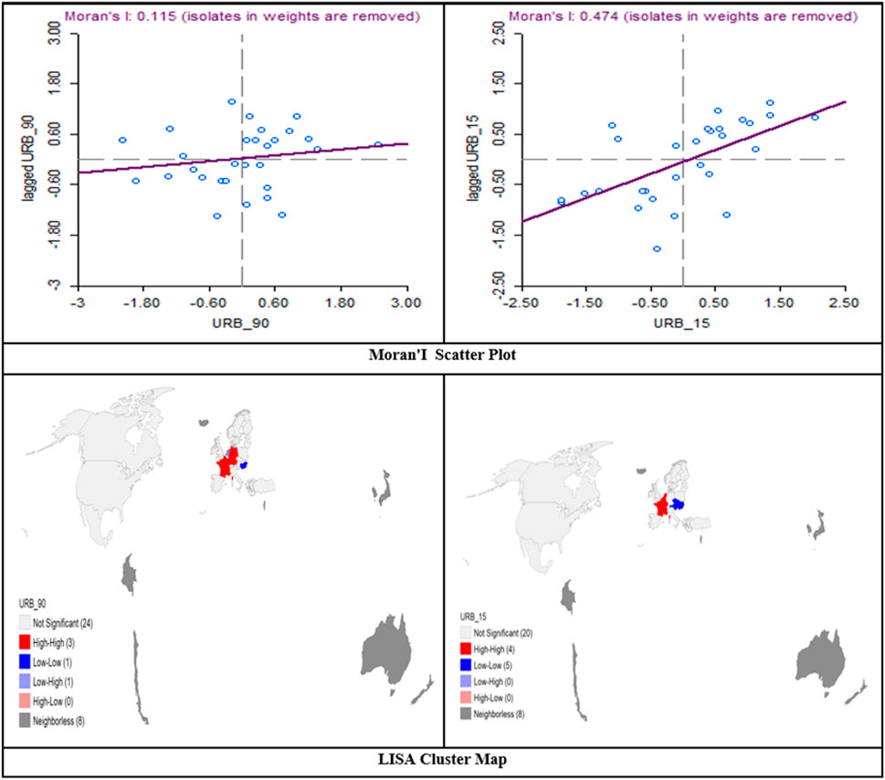
FIGURE 8. Moran Scatter Diagrams of URB data of OECD countries and LISA clustering maps for the period of 1990–2015.
LISA maps show that France, Germany, and Luxembourg were clustered in HH, Hungary in LL, in the Netherlands in LH in 1990. In 2015, Austria, Czech Republic, Hungary, Slovakia, and Slovenia were clustered in LL, whereas Belgium, France, Luxembourg, and the Netherlands were clustered in HH. For the KO variable, while the Netherlands was clustered in LH in 1990, it was clustered as HH in 2015. While Belgium was not included in any cluster in 1990, it was clustered in HH in 2015. Austria, Czech Republic, Slovakia, and Slovenia were not included in any cluster in 1990, but clustered in LL in 2015.
Figure 9 shows that Moran I value of DAE variable was calculated to be 0.119 in 1990 and 0.096 in 2015. It was determined that there was positive autocorrelation between countries in terms of the DAE variable.
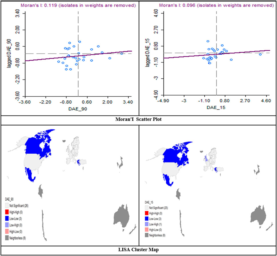
FIGURE 9. Moran Scatter Diagrams of openness index (DAE) data of OECD countries and LISA clustering maps for the period of 1990–2015.
LISA maps shows that Canada, Greece, and Mexico were clustered in LL in 1990 by the DAE variable. In 2015, Canada, Greece, and Mexico were clustered in LL, and the United Kingdom in LH. In 1990, the United Kingdom was not clustered in any cluster. The United Kingdom was clustered in LH in 2015.
Least Squares (LS) method in regression analysis is a statistical method that aims to minimize the sum of squares of error. In this study, while the CO2 emission rate was accepted as the dependent variable for the years 1990 and 2015, the ENK, GDP, URB, and DAE variables were considered as independent variables. The estimation results regarding the parameters of the model are as follows (Tables 1, 2).
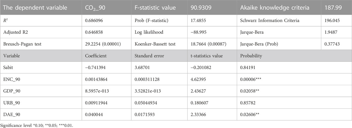
TABLE 1. Regression model results of 1990 data.
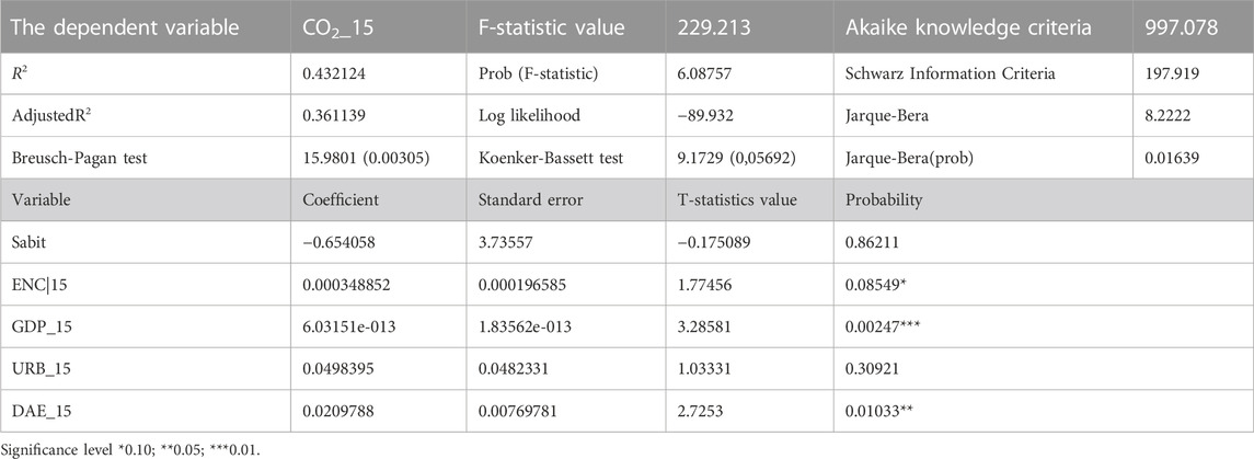
TABLE 2. Regression model results of 2015 data.
It was determined that, on CO2 emissions, the GDP and URB variables were significant at the confidence level of 90%, while the other variables were not statistically significant. In the model established for the data of the year 1990, the error variances must have an equal and normal distribution in order for the LCC estimations to be valid and for the model to be used. For the normality test of error variances, the relevant assumptions in this model were met considering the Jarque-Bera test results. Given the Breusch-Pagan and Koenker-Bassett test results for the varying variance, the model met the relevant assumptions. Error variances of the model have an equal and normal distribution.
It was determined that, considering the CO2 emission, the GDP was statistically significant in the 99% confidence interval, and other variables were not statistically significant. In the model established for 2015 data, the error variances must have equal and normal distribution in order for the LCC estimations to be valid and for the model to be used. For the normality test of error variances, the relevant assumptions in this model were met according to the Jarque-Bera test results. Considering the Breusch-Pagan and Koenker-Bassett test results for the varying variance, the model met the relevant assumptions. Error variances of the model have equal and normal distribution.
Considering the fact that the data used in the application belong to OECD countries and their geographical locations are taken into account, it is thought that it might contain spatial dependence since it might be affected by neighborhood relations. Thus, it was investigated whether there is a spatial dependence of the countries in terms of green economic indicators (CO2, ENC, GDP, URB and DAE), taking into account the neighborhood relationships of the countries. For this purpose, spatial dependency tests were conducted. Spatial dependency test results are shown in the Tables 3, 4 below.
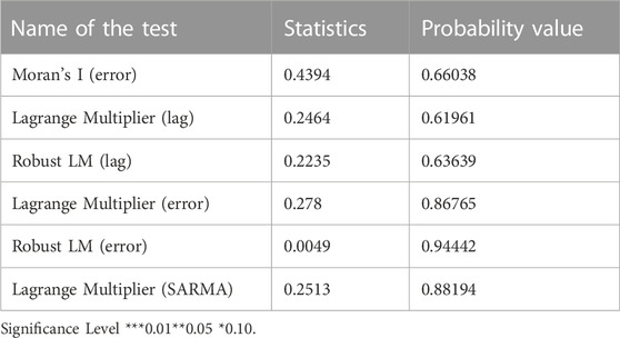
TABLE 3. Spatial dependency test results for 1990 data.
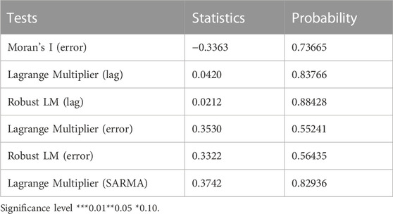
TABLE 4. Spatial dependency test results for 2015 data.
For the Moran I test statistic, the probability value was calculated to be 0.66038. Since this value is higher than 0.01, the H0 hypothesis, which states that there is no spatial dependence, is accepted. Although it was determined that there is no spatial dependence in OECD countries for 1990 data, the Moran I test does not provide information about the structure of spatial dependence. Examining the LM test values in the spatial dependence tests for the 1990 data, it was determined that they were not statistically significant. Thus, the interpretation should be made using the results of the regression analysis.
In Moran I test statistic, the probability value was calculated to be 0.73665. Since this value is higher than 0.1, H0, which indicates that there is no spatial dependence, is accepted. For the data of the year 2015, it was determined that there is no spatial dependence in OECD countries. For the same year, it was also determined that they were not statistically significant when the spatial dependence tests and LM test values were examined. Thus, the results of the regression analysis should be taken into account.
Given the results of the 1990 and 2015 regression analysis, there is a significant relationship between the dependent variable CO2 and the variables ENC, GDP, and DAE. The URB variable does not have a significant relationship. Considering the 1990 data, ENC variable was found to be 0.01, GDP and DAE variables are statistically significant at the significance level of 0.05. Considering the data for the year 2015, ENC, DAE, and GDP variables are significant at the significance levels of 0.1, 0.05, and 0.01, respectively. ENC, GDP, and DAE variables are positively related to the CO2 variable.
The present study was carried out by conducting spatial analysis and geographical regression analysis. All the OECD countries were examined individually. The results achieved from the methods used are explained comparatively. Since multiple countries and multiple variables were used in this study, the data were gathered from the World Bank for the period until 2015 and it poses a limitation for this study. However, it would be an honor for us if the current study team will be included in future studies. The results achieved here are explained below.
1) Comparing the data of the years 1990 and 2015, CO2 emissions increased in Japan, Korea, New Zealand, and Norway. On the other hand, the CO2 emissions decreased in Denmark, France, Germany, and Hungary. Considering the energy usage rates; Comparing the years 1990 and 2015 are compared, ENC rates increased in Austria, Israel, Japan, Korea, Slovenia and Spain. It decreased in Estonia, Hungary, Latvia, Lithuania, Slovakia, Switzerland, United Kingdom. In 1990 and 2015, GDP decreased in Denmark, Hungary, and Mexico but increased in Chile, Korea, and Poland. No changes were observed in other countries. The reason for this is estimated to be that the countries examined here consist of high- and upper-middle-income countries. Given the data on urbanization rates of OECD countries, URB decreased in Australia, Czech Republic, Estonia, Latvia, Lithuania, New Zealand, Spain, and Switzerland in 1990 and 2015. However, it increased in Colombia, Hungary, Italy, Japan, the Netherlands and Norway, and Turkey. Considering the DAE indicators, DAE decreased in 1990 and 2015 in Chile, Germany, Israel, Latvia, Lithuania, New Zealand, Norway, Switzerland, and the United Kingdom. It increased in the Czech Republic, Greece, Hungary, Mexico, Poland, Spain, and Sweden. The distributions of the maps of the variables in the form of increase, decrease and remaining constant are given in Table 5.
2) Examining the Moran scatter diagrams and LISA clustering maps of the variables, the spatial interactions of the variables with map distributions and visually regional differences are examined with Moran scatter diagrams. In addition, LISA analysis, which is a local indicator of spatial relationship, was used to examine if the observation values show regionally significant spatial clustering or segregation. Considering the Moran I scatter diagrams, for the CO2 emission data, Moran I value was found to be 0.121 in 1990 and 0.187 in 2015. These values indicate that there was a positive autocorrelation between the CO2 emission values of the countries. It was found that autocorrelation increased in 2015. Moran I value of ENC ratio variable was determined to be 0.313 in 1990 and 0.486 in 2015. These results show that there was a positive autocorrelation between the values of the countries. It was also found that autocorrelation increased in 2015. Moran I value of GDP variable was calculated to be 0.012 in 1990 and 0.035 in 2015. Considering the GDP variable, it was determined that there was positive autocorrelation between countries. While the Moran I value of the URB variable was 0.115 in 1990, this ratio increased to 0.474 in 2015. It was determined that there was positive autocorrelation between countries for the URB variable. Moran I value of DAE variable was calculated to be 0.119 in 1990 and 0.096 in 2015. It was determined that there was positive autocorrelation between countries for the DAE variable.
3) When the Lisa maps of the variables are examined, the countries can be grouped into four clusters in the LISA analysis at the significance level of 1%, these are HH, LH, LL, and HL. Moran scatter diagrams and LISA clustering maps (Figures 5–9) for the years 1990 and 2015 for the green economy indicators of OECD countries are given separately.
4) In the last stage, the Least Squares (LS) method, a statistical method aiming to make the sum of squares of the error the smallest, was used in the regression analysis. In this study, while the CO2 emission rate was accepted as the dependent variable for the years 1990 and 2015, the ENK, GDP, URB and DAE variables were considered as independent variables. The estimation results regarding the parameters of the model were found to be as follows. It was determined that the GDP and URB variables were significant in the confidence interval of 90% for the 1990 CO2 emissions, while the other variables were not statistically significant. It was determined that, regarding CO2 emissions, the GDP was significant at the confidence interval of 99% and other variables were not statistically significant. In the model established for the 1990 and 2015 data, the error variances must have equal and normal distribution in order for the LCC estimates to be valid and for the model to be used. For the normality test of error variances, the relevant assumptions in this model were met according to the Jarque-Bera test results. Considering the Breusch-Pagan and Koenker-Bassett test results for the varying variance, the model met relevant assumptions. Error variances of the model have equal and normal distribution.
5) It is thought that the data used in the application may be affected by neighborhood relations and may contain spatial dependence due to the locations of OECD countries. In this direction, it has been investigated whether the countries have spatial dependence in terms of neighbor relations in terms of green economic indicators (CO2, ENC, GDP, URB and DAE). It was concluded that there was no spatial dependence between the 1990 and 2015 data. The null hypothesis was accepted for both periods. According to the results of the 1990 and 2015 regression analysis, there is a significant relationship between the CO2 dependent variable and the ENC, GDP and DAE variables. The URB variable does not have a significant relationship. According to 1990 data, ENC variable is 0.01, GDP and DAE variables are significant at 0.05 significance level. According to the data in 2015, ENC, DAE and GDP variables are significant at 0.1, 0.05 and 0.01 significance levels, respectively. ENC, GDP and DAE variables are positively related to the CO2 variable.
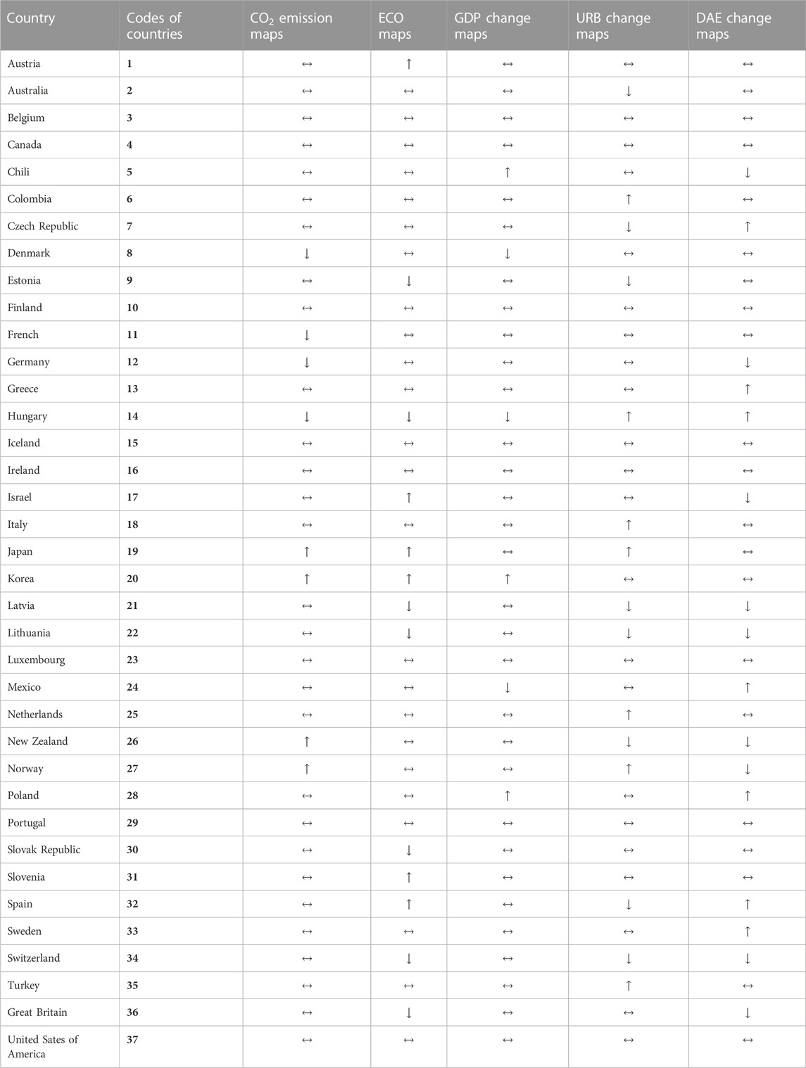
TABLE 5. Change directions of the maps of the variables.
The world have been facing a major environmental disaster in the last century. Temperatures are rising rapidly, precipitation cycles are changing, and glaciers and snow are melting, raising seawater levels on a global scale. Both natural processes and human activities create greenhouse gases. The most important natural greenhouse gas in the atmosphere is the water vapor. However, human activities cause the release of large amounts of greenhouse gases, increasing the atmospheric concentrations of these gases, which increases the greenhouse effect and also increases the temperature. It is essential to reduce these emissions in order to mitigate the climate change. Emergency measures were discussed at the United Nations Climate Change Conference held in Glasgow, Scotland, between 31 October and 12 November 2021. The world has warmed by 1°C when compared to the pre-industrial period and only 1°C more increase in the temperature cannot be tolerated. Therefore, environmental problems are core problems not only in developed, developing, or underdeveloped countries, but all the countries. However, China, the USA, and the European Union countries, which increase pollution the most, rank the first three globally. In addition, it causes a dramatic increase in pollution in underdeveloped countries.
Since the present study covers OECD countries and all of these countries are developed and upper-middle-income developing countries, no significant changes were observed in the findings of the countries. In addition, the data covering a period of 25 years poses a time constraint. However, it is hoped that it will be a stepping stone for comparison in future studies or combinations of different countries. Countries whose carbon dioxide emissions are clustered in HH, HL should give importance to environmental measures on the basis of policies. There is an increase in CO2 emissions throughout the study. Countries with the highest increase in CO2 include Japan, Korea, New Zealand and Norway.
The relationship between income growth and pollution, which the present study aims to prove as the reason for CO2 emission, is a common problem not only for OECD countries, but also for the whole world. In addition, considering the critical warnings mentioned above, the issue is too serious to be left to the initiatives of states. For this reason, it is essential for states to immediately implement practices that are supported by sanctions and include obligations, rather than basing the process on a voluntary basis, in order to protect the environment. From this point of view, the following suggestions can be taken into account on what should be done to reduce CO2 emissions all over the world.
Although developments advance technology and make our lives easier, green growth should be preferred in order to reduce its negative impact on CO2 emissions. Growth and sustainability should be made the fundamental principles in every field of life and every sector. In doing so, priority should be given to advancements in areas that significantly affect CO2 emissions. For example, transportation preferences should be quickly harmonized with nature. In particular, air transportation is one of the factors that cause the most CO2 emissions in the world. All transportation systems, especially airlines, should be taken under control with policies such as mode of transportation and pricing according to distance, in a way that will reduce CO2 emissions. This should be implemented as a sustainability policy, not a restriction on freedom. The share of fossil fuels in energy consumption should be reduced and the use of clean energy sources such as solar, wind, and biomass energy should be promoted. People should use their nutritional preferences towards organic and local agricultural products instead of products such as meat, refined oil, alcohol, and sugar. Disposable products should not be used outside, except for the case of preventing risk factors. Consumption of need rather than consumption of desire should be a way of life. Sorting garbage, eliminating wild landfills, and supporting recycling should be involved in the immediate action plans. In addition, laws should be made use of when necessary in order to reintroduce organic wastes to the soil and to prevent the natural resources from pollution. The usage period (except for single-use) of products should be applied not only for electronic goods but also for all products with multiple uses.
It is clear that it is not sustainable for people in the world to continue living upon the same habits. Even if a series of decisions have been taken in the studies on the environment, most of them could not yield the desired results due to the non-participation of the big states or the states that have implemented the practice later for economic or political reasons. For instance, Australia, Canada, Japan, and Russia, which had taken on commitments for the First Commitment Period of the Kyoto Protocol, did not taken on any commitment for the Second Commitment Period. The Second Commitment Period (Doha Amendment) of the Kyoto Protocol, which was signed by 144 participating countries, came into effect on 31 December 2020. Due to the initiation of the ‘Paris Agreement’ that governs the climate regime post-2020, the Second Commitment Period has only been symbolically acknowledged. As a result, the Kyoto Protocol has fulfilled its role as the initial implementation tool of the Framework Convention on Climate Change (unfccc.int/kyoto_protocol). Binding policies under the auspices of the United Nations can ensure collective action by all countries. This could lead to a general improvement. Otherwise, the chances of success for isolated policies remain slim.
This study, while potentially paving the way for future research, also has certain limitations. Firstly, there is a data limitation in the present study. Due to missing data in the World Bank database during the period the study was carried out, data was only obtained up to 2015, and it was not possible to access data for the year of 2020, which was targeted. Therefore, regarding data availability for other countries in future research, different country combinations and longer time frames could be tested. Secondly, in environmental studies, a model incorporating various variables affecting pollution can be constructed, and the spatial analysis method can be tested again. Finally, comparative analysis can be done by making use of the methods used in environmental studies, primarily the Environmental Kuznets Curve Hypothesis.
The original contributions presented in the study are included in the article/supplementary materials, further inquiries can be directed to the corresponding author.
AÇ: Conceptualization, Methodology, Software, Verification, Formal analysis, Research, Data enhancement, Writing–original draft, Writing–reviewing and organizing, Illustration. YA: Conceptualization, Verification, Analysis, reviewing, and organizing, Examination. All authors contributed to the article and approved the submitted version.
The authors would like to thank their colleagues, who have assisted in bringing the study to this stage and in the development of the paper, for their valuable comments and suggestions.
The authors declare that the research was conducted in the absence of any commercial or financial relationships that could be construed as a potential conflict of interest.
All claims expressed in this article are solely those of the authors and do not necessarily represent those of their affiliated organizations, or those of the publisher, the editors and the reviewers. Any product that may be evaluated in this article, or claim that may be made by its manufacturer, is not guaranteed or endorsed by the publisher.
1The present study was derived from the second section of the thesis completed in the year 2022 and titled “OECD Ülkelerinde Çevresel Kuznets Eğrisi Hipotezinin Testi ve Mekansal Analizi (Test and Spatial Analysis of Environmental Kuznets Hypothesis in the OECD Countries)” (Çay Atalay, 2022).
Abbasi, M. A., Parveen, S., Khan, S., and Kamal, M. A. (2020). Urbanization and energy consumption effects on carbon dioxide emissions: Evidence from asian-8 countries using panel data analysis. Environ. Sci. Pollut. Res. 27, 18029–18043. doi:10.1007/s11356-020-08262-w
Acar, S., and Lindmark, M. (2017). Convergence of CO2 emissions and economic growth in the OECD countries: Did the type of fuel matter? Energy Sources, Part B Econ. Plan. Policy 12 (7), 618–627. doi:10.1080/15567249.2016.1249807
Akay, A., Martinsson, P., and Ralsmark, H. (2019). Relative concerns and sleep behavior. Clim. Change Train. Modul. Ser. 15, 1–14. doi:10.1016/j.ehb.2018.12.002
Alkan, Ö., and Albayrak, Ö. K. (2020). Ranking of renewable energy sources for regions in Turkey by fuzzy entropy based fuzzy COPRAS and fuzzy MULTIMOORA. Renew. Energy 162, 712–726. doi:10.1016/j.renene.2020.08.062
Ansari, M. A., Haider, S., and Khan, N. A. (2019). Does trade openness affects global carbon dioxide emissions: Evidence from the top CO2 emitters. Manag. Environ. Qual. Int. J. 31, 32–53. doi:10.1108/meq-12-2018-0205
Anselın, L., and Rey, S. (1991). Properties of tests for spatial dependence in linear regression models. Geogr. Anal. 23 (2), 112–131. doi:10.1111/j.1538-4632.1991.tb00228.x
Anselin, L. (1998). “ExploratorySpatial data analysis in a geocomputational environment,” in Geocomputation, a primer (New York, NY, USA: Wiley), 77–94.
Anselin, L. (1988). Lagrange multiplier test diagnostics for spatial dependence and spatial heterogeneity. Geogr. Anal. 20 (1), 1–17. doi:10.1111/j.1538-4632.1988.tb00159.x
Anselin, L., and Rey, J. S. (2014). Modern spatial econometrics in practice. Chicago, IL, USA: GeoDa Press LLC.
Anselın, L. (1992). Spatial Data Analysis With GIS: An Introduction To Application İn The Social Sciences, National Center for Geographic Information and Analysis (Technical Report 92/10). Santa Barbara, Ca, USA: University of California.
Anselin, L. (1996). “The Moran scatterplot as an ESDA tool to assess local instability in spatial association,” in Spatial analytical perspectives on GIS. Editors M. Fischer, H. J. Scholten, and D. Unwin (London, UK: Taylor and Francis), 111–125.
Anser, M. K., Usman, M., Godil, D. I., Shabbir, M. S., Sharif, A., Tabash, M. I., et al. (2021). Does globalization affect the green economy and environment? The relationship between energy consumption, carbon dioxide emissions, and economic growth. Environ. Sci. Pollut. Res. 28 (37), 51105–51118. doi:10.1007/s11356-021-14243-4
Aral, N. (2016). Spatial analysis of unemployment in Turkey. Published Master's Thesis. Bursa, Turkey: Uludag University Institute of Social Sciences.
Asumadu-Sarkodie, S., and Owusu, P. A. (2016). A multivariate analysis of carbon dioxide emissions, electricity consumption, economic growth, financial development, industrialization, and urbanization in senegal. Energy Sources, Part B: Economics, Planning, And Policy, 12(1), 77-84. doi:10.1080/15567249.2016.1227886
Asumadu-Sarkodie, S., and Owusu, P. A. (2017). The causal effect of carbon dioxide emissions, electricity consumption, economic growth, and industrialization in Sierra Leone. Energy Sources, Part B Econ. Plan. Policy 12 (1), 32–39. doi:10.1080/15567249.2016.1225135
Azam, (2019). Relationship between energy, investment, human capital, environment, and economic growth in four BRICS countries. Environ. Sci. Pollut. Res. 26, 34388–34400. doi:10.1007/s11356-019-06533-9
Başar, Ö. D. (2009). Spatial regression analysis, statistics. PhD Thesis. Istanbul, Turkey: Mimar Sinan University Institute of Science and Technology.
Bivand, R. S., and Wong, D. W. (2018). Comparing implementations of global and local indicators of spatial association. Test 27 (3), 716–748. doi:10.1007/s11749-018-0599-x
Çamkaya, S., Karaaslan, A., and Uçan, F. (2022). Investigation of the effect of human capital on environmental pollution: Empirical evidence from Turkey. Environ. Sci. Pollut. Res. 30, 23925–23937. doi:10.1007/s11356-022-23923-8
Çay Atalay, A. (2022). Testing of the environmental kuznets curve hypothesis and spatial analysis in OECD countries (Thesis No. 737107). PhD thesis. Atatürk University, YÖK Thesis Center. Available at: https://tez.yok.gov.tr/UlusalTezMerkezi/tezSorguSonucYeni.jsp#top2.
Chen, L., Zhang, X., He, F., and Yuan, R. (2019). Regional green development level and its spatial relationship under the constraints of haze in China. J. Clean. Prod. 210, 376–387. doi:10.1016/j.jclepro.2018.11.037
Clıff, A., and Keith, O. (1972). Testing for spatial autocorrelation among regression residuals. Geogr. Anal. 4 (3), 267–284. doi:10.1111/j.1538-4632.1972.tb00475.x
Fan, B., Zhang, Y., Li, X., and Miao, X. (2019). Trade openness and carbon leakage: Empirical evidence from China’s industrial sector. Energies 12 (6), 1101. doi:10.3390/en12061101
Fıscher Manfred, M., and Jinfeng, W. (2011). Spatial data analysis: Models, methods and techniques. Berlin, Germany: Springer.
Guo, B., Feng, Y., and Hu, F. (2023). Have carbon emission trading pilot policy improved urban innovation capacity? Evidence from a quasi-natural experiment in China. Environ. Sci. Pollut. Res., 1–14. doi:10.1007/s11356-023-25699-x
Gwartney, J. D., Stroup, R. L., Russell, S., and Sobel, M. D. (2010). Macroeconomics: Private and public choice. Boston, Massachusetts, United States: Cengage Learning.
Hasnisah, A., Azlina, A. A., and Taib, C. M. I. C. (2019). The impact of renewable energy consumption on carbon dioxide emissions: Empirical evidence from developing countries in Asia. Int. J. Energy Econ. Policy 9 (3), 135–143. doi:10.32479/ijeep.7535
Huang, Q., Hu, Y., and Luo, L. (2022). Spatial analysis of carbon dioxide emissions from producer services: An empirical analysis based on panel data from China. Environ. Sci. Pollut. Res. 29 (35), 53293–53305. doi:10.1007/s11356-022-19590-4
Iqbal, N., Abbasi, K. R., Shinwari, R., Guangcai, W., Ahmad, M., and Tang, K. (2021). Does exports diversification and environmental innovation achieve carbon neutrality target of OECD economies? J. Environ. Manag. 291, 112648. doi:10.1016/j.jenvman.2021.112648
Jezierska-Thöle, A., Gwiaździńska-Goraj, M., and Dudzińska, M. (2022). Environmental, social, and economic aspects of the green economy in polish rural areas—a spatial analysis. Energies 15 (9), 3332. doi:10.3390/en15093332
Khan, Z., Shahbaz, M., Ahmad, M., Rabbi, F., and Siqun, Y. (2019). Total retail goods consumption, industry structure, urban population growth and pollution intensity: An application of panel data analysis for China. Environ. Sci. Pollut. Res. 26, 32224–32242. doi:10.1007/s11356-019-06326-0
Khoshnevis Yazdi, S., and Golestani Dariani, A. (2019). CO2 emissions, urbanisation and economic growth: Evidence from asian countries. Econ. research-Ekonomska istraživanja 32 (1), 510–530. doi:10.1080/1331677x.2018.1556107
Kirikkaleli, D., and Adebayo, T. S. (2021). Do public-private partnerships in energy and renewable energy consumption matter for consumption-based carbon dioxide emissions in India? Environ. Sci. Pollut. Res. 28 (23), 30139–30152. doi:10.1007/s11356-021-12692-5
Kuznets, S. (1955). “International differences in capital formation and financing,” in Capital formation and economic growth (Princeton, New Jersey, United States: Princeton University Press), 19–111.
LeSage, J., and Pace, R. K. (2009). Introduction to spatial econometrics. Boca Raton, Florida, United States: Chapman and Hall/CRC.
Liu, J., Li, Z., Dong, C., and Sriboonchitta, S. (2019). “The impact of economic growth, energy consumption and trade openness on carbon emissions: An empirical analysis in China,” in International symposium on integrated uncertainty in knowledge modelling and decision making (Cham, Germany: Springer), 235–244.
Lv, Z., and Xu, T. (2019). Trade openness, urbanization and CO2 emissions: Dynamic panel data analysis of middle-income countries. J. Int. Trade and Econ. Dev. 28 (3), 317–330. doi:10.1080/09638199.2018.1534878
Maroufi, N., and Hajilary, N. (2022). The impacts of economic growth, foreign direct investments, and gas consumption on the environmental Kuznets curve hypothesis CO2 emission in Iran. Environ. Sci. Pollut. Res. 29 (56), 85350–85363. doi:10.1007/s11356-022-20794-x
Mutascu, M. (2018). A time-frequency analysis of trade openness and CO2 emissions in France. Energy policy 115, 443–455. doi:10.1016/j.enpol.2018.01.034
Niu, H., and Lekse, W. (2017). “Carbon emission effect of urbanization at regional level: Empirical evidence from China,” in Economics discussion papers (Kiel, Germany: Kiel Institute for the World Economy), 62.
Nurgazina, Z., Ullah, A., Ali, U., Koondhar, M. A., and Lu, Q. (2021). The impact of economic growth, energy consumption, trade openness, and financial development on carbon emissions: Empirical evidence from Malaysia. Environ. Sci. Pollut. Res. 28 (42), 60195–60208. doi:10.1007/s11356-021-14930-2
Ord, J. K. (1975). Estimation methods for models of spatial interaction. Amer. Stat. Assoc. 70, 120–126. doi:10.1080/01621459.1975.10480272
Ponce, P., and Khan, S. A. R. (2021). A causal link between renewable energy, energy efficiency, property rights, and CO2 emissions in developed countries: A road map for environmental sustainability. Environ. Sci. Pollut. Res. 28, 37804–37817. doi:10.1007/s11356-021-12465-0
Sahin, Ü. (2015). Green economy, green politics series (electronic book). Istanbul, Turkey: Yeni Insan Publishing House.
Salahuddin, M., Alam, K., Ozturk, I., and Sohag, K. (2018). The effects of electricity consumption, economic growth, financial development and foreign direct investment on CO2 emissions in Kuwait. Renew. Sustain. Energy Rev. 81 (P2), 2002–2010. doi:10.1016/j.rser.2017.06.009
Shang, Y., Lian, Y., Chen, H., and Qian, F. (2023). The impacts of energy resource and tourism on green growth: Evidence from asian economies. Resour. Policy 81, 103359. doi:10.1016/j.resourpol.2023.103359
Shao, L., Yu, X., and Feng, C. (2019). Evaluating the eco-efficiency of China's industrial sectors: A two-stage network data envelopment analysis. J. Environ. Manag. 247, 551–560. doi:10.1016/j.jenvman.2019.06.099
Union National Environment Programme (2011). Union national environment programme. https://www.unep.org/unepmap/.
Velame, I. S., and Teixeira, J. R. (2017). Green economy and sustainable development: The Latin America scenario. Erud. e-Journal World Acad. Art Sci. 2 (3), 28–38.
World Bank (2019). World Bank. https://data.worldbank.org/topic/19.
Xing, Z., Huang, J., and Wang, J. (2023). Unleashing the potential: Exploring the nexus between low-carbon digital economy and regional economic-social development in China. J. Clean. Prod. 413, 137552. doi:10.1016/j.jclepro.2023.137552
Yang, Y., Zhou, Y., Poon, J., and He, Z. (2019). China's carbon dioxide emission and driving factors: A spatial analysis. J. Clean. Prod. 211, 640–651. doi:10.1016/j.jclepro.2018.11.185
Zeren, F. (2011). Spatial econometrics and spatial Panel econometric approaches: An application on income convergence hypothesis for EU member states. Published Doctoral Thesis. Istanbul, Turkey: Istanbul University Institute of Social Sciences.
Zhao, M., Liu, F., Song, Y., and Geng, J. (2020). Impact of Air pollution regulation and technological investment on sustainable development of green economy in Eastern China: Empirical analysis with panel data approach. Sustainability 12 (8), 3073. doi:10.3390/su12083073
Keywords: OECD countries, spatial analysis, LISA analysis, green economy, autocorrelation, regression analysis
Citation: Çay Atalay A and Akan Y (2023) The spatial analysis of green economy indicators of OECD countries. Front. Environ. Sci. 11:1243278. doi: 10.3389/fenvs.2023.1243278
Received: 20 June 2023; Accepted: 22 September 2023;
Published: 13 October 2023.
Edited by:
Ulas Akkucuk, Boğaziçi University, TürkiyeCopyright © 2023 Çay Atalay and Akan. This is an open-access article distributed under the terms of the Creative Commons Attribution License (CC BY). The use, distribution or reproduction in other forums is permitted, provided the original author(s) and the copyright owner(s) are credited and that the original publication in this journal is cited, in accordance with accepted academic practice. No use, distribution or reproduction is permitted which does not comply with these terms.
*Correspondence: Ayşe Çay Atalay, YXlhdGFsYXlAYXRhdW5pLmVkdS50cg==
†ORCID: Ayşe Çay Atalay, orcid.org/0000-0002-3600-368X; Yusuf Akan, orcid.org/0000-0002-2446-5043
Disclaimer: All claims expressed in this article are solely those of the authors and do not necessarily represent those of their affiliated organizations, or those of the publisher, the editors and the reviewers. Any product that may be evaluated in this article or claim that may be made by its manufacturer is not guaranteed or endorsed by the publisher.
Research integrity at Frontiers
Learn more about the work of our research integrity team to safeguard the quality of each article we publish.