
95% of researchers rate our articles as excellent or good
Learn more about the work of our research integrity team to safeguard the quality of each article we publish.
Find out more
ORIGINAL RESEARCH article
Front. Environ. Sci. , 31 August 2023
Sec. Environmental Informatics and Remote Sensing
Volume 11 - 2023 | https://doi.org/10.3389/fenvs.2023.1240106
This article is part of the Research Topic Remote Sensing for Environmental Monitoring View all 13 articles
 Tiago G. Morais1*
 Marjan Jongen1
 Camila Tufik2
 Nuno R. Rodrigues3Ivo Gama3
 João Serrano4Maria C. Gonçalves5Raquel Mano6Tiago Domingos1
 Ricardo F. M. Teixeira1
Introduction: Soil organic carbon (SOC) sequestration is one of the main ecosystem services provided by well-managed grasslands. In the Mediterranean region, sown biodiverse pastures (SBP) rich in legumes are a nature-based, innovative, and economically competitive livestock production system. As a co-benefit of increased yield, they also contribute to carbon sequestration through SOC accumulation. However, SOC monitoring in SBP require time-consuming and costly field work.
Methods: In this study, we propose an expedited and cost-effective indirect method to estimate SOC content. In this study, we developed models for estimating SOC concentration by combining remote sensing (RS) and machine learning (ML) approaches. We used field-measured data collected from nine different farms during four production years (between 2017 and 2021). We utilized RS data from both Sentinel-1 and Sentinel-2, including reflectance bands and vegetation indices. We also used other covariates such as climatic, soil, and terrain variables, for a total of 49 inputs. To reduce multicollinearity problems between the different variables, we performed feature selection using the sequential feature selection approach. We then estimated SOC content using both the complete dataset and the selected features. Multiple ML methods were tested and compared, including multiple linear regression (MLR), random forests (RF), extreme gradient boosting (XGB), and artificial neural networks (ANN). We used a random cross-validation approach (with 10 folds). To find the hyperparameters that led to the best performance, we used a Bayesian optimization approach.
Results: Results showed that the XGB method led to higher estimation accuracy than the other methods, and the estimation performance was not significantly influenced by the feature selection approach. For XGB, the average root mean square error (RMSE), measured on the test set among all folds, was 2.78 g kg−1 (r2 equal to 0.68) without feature selection, and 2.77 g kg−1 (r2 equal to 0.68) with feature selection (average SOC content is 13 g kg−1). The models were applied to obtain SOC content maps for all farms.
Discussion: This work demonstrated that combining RS and ML can help obtain quick estimations of SOC content to assist with SBP management.
Soil systems are intricate networks of both organic and inorganic matter with varying chemical and physical attributes that can differ from site to site, or even within the same site. These systems also serve as the primary carbon reservoirs on land, with a capacity to store roughly 80% of all organic carbon, totalling an estimated 2,400 Pg of carbon (PgC)—more than three times the amount found in the atmosphere (Jobbágy and Jackson, 2000; Chappell et al., 2016). The level of soil organic carbon (SOC) present is heavily influenced by soil management practices, soil properties, and climatic conditions, with significant spatial differences that pose a challenge when estimating terrestrial carbon stocks and fluxes (Giardina et al., 2014; Doetterl et al., 2015; Koven et al., 2017). In terms of preserving SOC and other essential ecosystem services, grasslands rank among the most significant terrestrial ecosystems (Egoh et al., 2016; Bardgett et al., 2021). However, SOC estimation in grassland ecosystems is challenging due to factors such as the high spatial and temporal variability of SOC, heterogeneous distribution within soil profiles and the fact that methods for SOC estimation are often destructive and time-consuming (Angelopoulou et al., 2019; Xiao et al., 2019). Remote sensing (RS) and machine learning (ML) models have the potential to improve the accuracy and certainty of SOC estimation in grassland ecosystems.
RS data is often used in providing explanatory variables for estimating SOC using ML methods (Angelopoulou et al., 2019), especially as spectral sensors have improved significantly in recent decades, with enhanced spatial and temporal resolutions. Consequently, RS data from satellites (such as Landsat 7/8 and Sentinel-2) and unmanned aerial vehicles (UAVs) have led to a rise in applications for monitoring SOC in croplands and grasslands (Zheng et al., 2004; Mariano et al., 2018; Sun et al., 2021). Vegetation indices, have been widely used to estimate SOC (Xu et al., 2008; Ullah et al., 2012; Davids et al., 2018), but there are limitations and uncertainties associated with their use (Zhao et al., 2014; Ali et al., 2016). More recently, individual spectral bands, sometimes in combination with VIs, have been used to indirectly estimate SOC (Wang et al., 2021; Zepp et al., 2021; Pan et al., 2022). RS data is often combined with other covariates such as terrain and climatic variables to improve the estimation (Mallik et al., 2020; Gardin et al., 2021; Wang et al., 2022).
In recent years, there has been an increased interest in using ML methods for estimating SOC or soil organic matter (SOM) (Pezzuolo et al., 2017; Angelopoulou et al., 2019; Odebiri et al., 2021; Biney, 2022; Chan et al., 2023). ML methods are automated techniques that look for hypotheses to explain data and can be applied to any learning task. Commonly used models to estimate SOC/SOM include random forests (RF) and artificial neural networks (ANNs) (Lamichhane et al., 2019). These models have demonstrated their capacity to enhance SOC estimation by reducing the error between the ground-measured SOC/SOM values and the estimates generated by the models (e.g., Ladoni et al., 2010; Pouladi et al., 2019; Zepp et al., 2021; Wang et al., 2022). Further, some ML methods such as RF have also demonstrated higher performance in estimating SOC than geospatial models (Veronesi and Schillaci, 2019). Estimations of SOC/SOM content at high spatial resolutions (<50 m) have significantly improved in the past decades (Angelopoulou et al., 2019). While ML methods are predominantly associated with the use of satellite data, there has been a limited number of studies exploring other remote sensing sources with higher spatial resolution, such as UAVs (Angelopoulou et al., 2019). Satellite data sources remain the most commonly used as they offer advantages such as short revisit times and medium spatial resolution (Xiao et al., 2019). However, most applications developed to estimate SOC/SOM content are still specific to the particular land cover systems in which they were trained and validated. For highly specific land use systems that can be a problem, as existing models were never trained with system-specific data.
Sown biodiverse permanent pastures rich in legumes (SBP) are one example of such unique grassland/pasture systems. SBP have been implemented since the 1960 s in Portugal to boost pasture yields and increase animal stocking rates (Teixeira et al., 2015; Morais et al., 2022). This system involves sowing a combination of up to 20 legume and grass species or cultivars that provide high-quality animal feed. In addition to the direct benefits of this system, such as increased forage production, a major co-benefit is soil carbon sequestration, as noted by Moreno et al. (2021) and Teixeira et al. (2011). To assist with compliance to the Kyoto Protocol goals under the Agriculture, Forestry and Other Land Uses activities, the Portuguese Carbon Fund provided support for the installation and maintenance of SBP between 2009 and 2014. Payments were made to over 1,000 farmers based on predetermined sequestration factors that were established from data gathered during previous studies, rather than on carbon content increases that were measured on the farm (Teixeira et al., 2011; APA, 2018). Thus, there is a lack of indirect methods that can be broadly applied and are specifically tailored to SBP systems, hindering effective carbon management of this unique pasture system.
In the present research, we employed a combination of RS data and various ML techniques to estimate SOC content at a depth of 20 cm in SBP. We collected data from Sentinel-1 and Sentinel-2 satellites during two periods, August and the closest date to soil sampling. Five VIs were extracted from the RS data, along with various climatic, soil, terrain, and other auxiliary variables. Two variable selection methods were used, one utilizing all variables and the other using the sequential feature selection (SFS) approach to measure multicollinearity among input variables and select the most relevant ones for the SOC estimation. We evaluated the performance of the models using a random cross-validation approach with 10 folds. The resulting models were then used to estimate SOC and generate SOC content maps for the sampled farms’ entire sites.
Data from nine different farms were used in this work: eight farms in Portugal (Farms 1, 2, 3, 5, 6, 7, 8, and 9) and one in Spain (Farm 4). They are located across latitudes and longitudes ranging respectively between 37°50′ and 40°30′N and 6°80′ and 8°30′W (Figure 1). The size of surveyed farms ranges between 26 ha (Farm 8) and 42 ha (Farm 6). All farms are in the hot-summer Mediterranean climate region, according to the Köppen climate classification system (Rubel and Kottek, 2010; IPMA, 2018).
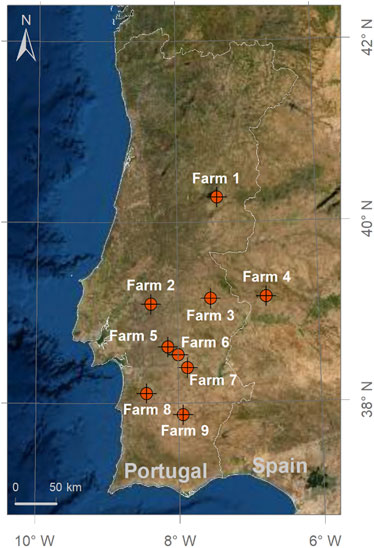
FIGURE 1. Location of the nine sampled farms used in this work. Farm 4 is the only one in Spain, all other farms being in Portugal.
According to the European Soil Database (ESDAC, 2003), the nine sampled farms are characterized by five different soil types: Dystric Cambisol (Farms 1 and 4), Orthic Podzol (Farms 2, 3, and 5), Eutric Cambisol (Farms 6 and 8), Rhodo-Chromic Luvisol (Farm 7) and Ferric Luvisol (Farm 9). Regarding dominant parent material, there are six different types: granite (Farms 1 and 6), diorite (Farms 3 and 5), acid regional metamorphic rocks (Farms 7 and 9), river terrace sand or gravel (Farm 2), (meta-) shale/argillite (Farm 4) and sandstone (Farm 8).
In total, four production years were covered in this study (between 2017-18 and 2020-21). The number of production years covered and the number of samples per production year vary between farms. For example, Farm 1 was sampled in all four production years, but Farm 9 was only sampled in one production year (2018-19). Additionally, considering only Farm 1, in the first year, 40 plots/locations were sampled, but in the following years, more samples were collected, with 2018-19 having the highest number of samples (75 samples). The total number of collected samples and collection years are summarized in Table 1. In each farm, the selection of sampling locations was carefully made to minimize any potential influence of trees and rocks on the measured SOC content. Due to the significantly different tree densities across the sampling locations, achieving an equal number of sampling locations per farm was not feasible.
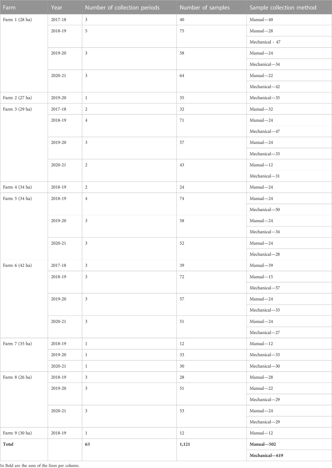
TABLE 1. Description of the collected soil samples per farm and production year.
Soil sampling took place in the period between September and May. They were collected using two different methods: 1) manual collection and 2) mechanical collection. This was expressed in the analysis as an auxiliary binary variable. In both collection methods, samples were collected in the 0–20 cm topsoil layer, which is the reference depth in the LUCAS Soil project conducted by the European Soil Data Centre (ESDAC)—Joint Research Centre (JRC) (Orgiazzi et al., 2018). Manual collection used an auger (2 cm diameter), while mechanical collection used a Wintex 2000 soil sampler installed on a utility terrain vehicle. Each soil sample was composed of four sub-samples that were pooled and mixed to achieve uniformity. All soil samples were air-dried and passed through a 2 mm stainless steel sieve. SOC content was calculated using the soil fractions after an elemental analysis performed after a combustion at 1050°C. In all soil samples, inorganic carbon removal was performed prior to the total SOC quantification. All values of SOC presented here are expressed in grams of SOC per kg of dry soil.
In this study, we used RS data, climate, terrain, and soil data to model SOC content. All data was obtained from Google Earth Engine (GEE), which reduced data processing time and storage space. GEE is a cloud-based platform that allows users to access and process massive amounts of geospatial data. The platform includes a catalogue of over 600 petabytes of satellite imagery, aerial imagery, and other geospatial datasets. GEE enables users to analyse data to track changes over time, map trends, and quantify differences on the Earth’s surface. For example, the complete Sentinel-2 database is available. Table 3 summarizes all the data used, including their sources, variable names, and spatial resolution. In total, 49 input variables were considered.
For all data used, we applied “min-max” normalization (i.e., values were normalized between 0 and 1). Each input was subjected to individual and independent data normalization, without any dependence on the other inputs. This was done to increase the learning rate and ensure faster convergence as models with large weights tend to be unstable and suffer from poor performance during learning and sensitivity to input values, the latter resulting in higher generalization error (Bishop, 1995; Goodfellow et al., 2016).
In order to understand the relationship between the data used and the measured SOC content, we calculated a Spearman’s rank correlation (Spearman, 1904). This is a non-parametric measure of monotonic statistical dependence between two variables, and it does not make any assumptions about the distribution of the variables.
The RS data were obtained from the Sentinel-1 and Sentinel-2 missions. We used the Sentinel-1 C-band Level-1 Ground Range Detected images provided by GEE, which were acquired on a descending orbit in Interferometric Wide swath mode (IW). The imagery in GEE consists of Level-1 Ground Range Detected (GRD). We utilized the VV and VH polarization bands, and the intensity cross-ratio (CR) VV/VH was also calculated. Sentinel-2 is a two-satellite constellation mission (Sentinel-2A and Sentinel-2B), which carries a wide-swath multispectral imager with 13 spectral bands. The image resolutions are 10 m (Blue, Green, Red, and Near Infrared bands), 20 m (three Vegetation Red Edge bands, Narrow NIR band, and two shortwave-infrared bands), and 60 m (Coastal aerosol, Water vapour, and SWIR-Cirrus bands). We used Level-2A data products, i.e., bottom of atmosphere (BOA) reflectance images obtained from Level-1C products. Bands 1 (coastal aerosol), 9 (water vapour), and 10 (SWIR-Cirrus) were excluded as they are specific to atmospheric characterization and not land surface monitoring. Besides the individual bands, we used spectral data to calculate five vegetation indices (Table 2): the normalized difference vegetation index (NDVI) (Tucker, 1979), normalized difference water index (NDWI) (Gao, 1996), simple ratio (SR), soil-adjusted vegetation index (SAVI) (Huete, 1988) and optimized soil-adjusted vegetation index (OSAVI) (Rondeaux et al., 1996).
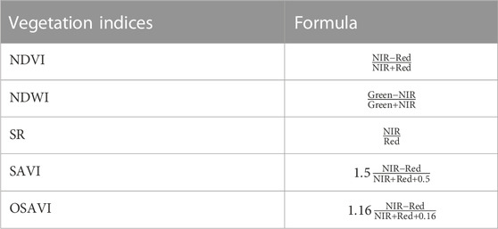
TABLE 2. Calculation formula for the vegetation indices used in this paper. NDVI, normalized difference vegetation index; NDWI, normalized difference water index; SR, simple ratio; SAVI, soil-adjusted vegetation index; OSAVI, optimized soil-adjusted vegetation index.
Regarding the Sentinel-1 and Sentinel-2 data, for each band or vegetation index, we considered data from two periods. First, we considered a composite image of the available images for the period between August 1st and August 31st. This composite image aims to capture the spectral reflectance of the bare soil. Second, we also considered data from Sentinel-1 and Sentinel-2 from the closest date to the soil collection date. This aims to capture the inter-yearly variation of SOC between the period when the soil was bare and the collection date, when the soil was covered by vegetation.
For the period when the soil is almost bare in the SBP system, i.e., during August, we considered a composite image of the available Sentinel-1 and Sentinel-2 images for the period between 1st August and 31st August. The composite image in August captures the spectral reflectance of the bare soil, and the image closest to the soil collection period captures the influence of vegetation on SOC. We also removed pixels masked as clouds and cloud shadow using the “pixel_qa” band from Sentinel-2 data obtained from GEE. Additionally, we also used the available image closest to each soil collection period. All the individual bands and the vegetation indices were calculated and downloaded using GEE.
The mineralization and accumulation of SOC are highly dependent on climate, specifically soil temperature and moisture (Rey et al., 2005; Thornton et al., 2009). Therefore, we used data from the Global Land Data Assimilation System (GLDAS—Rodell et al., 2004) for these variables. The data available in GLDAS is on a daily basis and we used both soil temperature and moisture on the collection date. We also included soil data to characterize SOC, such as clay, sand, silt content and soil pH (H2O). Soil data was obtained from SoilGrids (Hengl et al., 2017). SOC is also influenced by terrain characteristics (Rogge et al., 2018) and thus we used data from NASA EOSDIS Land Processes DAAC (NASA, 2020) and Theobald et al. (2015) for the Digital Elevation Model (DEM), the Continuous Heat-Insolation Load Index (CHILI), the Multi-Scale Topographic Position Index (mTPI) and Topographic Diversity (topoDivers). CHILI captures the effects of insolation and topographic shading on evapotranspiration (calculated by the insolation at early afternoon, sun altitude equivalent to the equinox). mTPI distinguishes ridge from valley forms (calculated by the elevation at each location subtracted by the mean elevation within a neighborhood). Finally, topoDivers represents the variety of temperature and moisture conditions available to species as local habitats (calculated by mTPI and soil moisture). All data was calculated and downloaded using GEE.
We also considered six additional auxiliary variables: the number of days since the beginning of the production year (counting from 31st August), the number of days between the closest Sentinel-2 image and the soil sampling date, the number of days between the closest Sentinel-1 image and the soil sampling, the collection method (manual or mechanical) the year, and the month.
In this study, we used a long list of independent variables (49 inputs) to estimate SOC content. However, in practice not all of those variables might be relevant for estimating SOC. To address this, we used a two-step approach: 1) first, all input variables were included in the estimation of SOC, then 2) we applied SFS and retrained the algorithm with a subset of variables. The SFS approach involves adding features in an automated and iterative manner to form a feature subset. At each iteration, the best feature to add or remove is chosen based on the cross-validation score of the model validation procedure. Then, after applying SFS, we obtained a subset of the input data that has the most relevant variables for estimating SOC. This method allowed us to identify and select only the pertinent variables that are crucial for accurately estimating SOC content within the dataset.
The SOC content was modelled using four regression methods: multiple linear regression (MLR—Barbur et al., 1994), random forest (RF—Breiman, 2001), extreme gradient boosting (XGBoost- XGB—Chen and Guestrin, 2016) and artificial neural network (ANN—Rumelhart et al., 1986). To optimize the regression models, we used Bayesian optimization with 100 initializations to find the best hyperparameters for each method. The methods and their respective hyperparameter option spaces are described in detail in the next section. All methods were implemented on Python 3.8.4, using multiple toolboxes. For MLR regression and RF, we used the scikit-learn 0.24 toolbox (https://github.com/scikit-learn/scikit-learn). For XGB, we used the xgboost 1.4.2 toolbox (https://github.com/dmlc/xgboost). For ANN, keras 2.9 was used to construct the ANN architecture and TensorFlow 2.7 as the backend for keras (https://github.com/keras-team/keras; https://github.com/tensorflow/tensorflow). To prepare the data, we used Numpy 1.18.5 (https://github.com/numpy/numpy) and Pandas 1.0.4 (https://github.com/pandas-dev/pandas). The Bayesian optimization was performed using the scikit-optimizer 0.8.1 (https://github.com/scikit-optimize/scikit-optimize).
MLR was the simplest method used in this study. It fits a linear equation to the observed data using the relationship between all independent variables and a dependent variable, using a least squares fit. Decision trees/forests, such as RF, is a learning method that creates multiple decision trees and fits the trees to training data. In a RF, the value of the response variable can change across the trees in the forest. However, within each individual tree, the predicted variable does not change in each leaf. This is because each tree is built using the same set of predictor variables and the same splitting criteria, resulting in consistent splits at each node of the tree. One advantage of RF over other bagging models is its ability to produce nearly uncorrelated predictions due to the random features, producing predictions with low variance. For optimization, we tested various options involving the number of estimators, the minimum number of samples per leaf, the maximum depth, the error function, the maximum number of features/inputs in each split, and the use of a bootstrap approach.
XGB is a newer method, proposed in 2016, that is based on gradient boosting tree methods. It trains by making predictions sequentially and combining weak predictive tree models, learning from the obtained errors. XGB has significant improvements to traditional gradient boost methods, namely, in terms of performance, parallelization, distributed computing, and computational time. For optimization, various options such as the number of estimators, the learning rate, the maximum depth of the trees, and L1 and L2 regularization were considered.
An artificial neural network (ANN) is a multi-layer network structure that consists of an input layer with a set of input/explanatory variables, an output layer containing the dependent/objective variable, and one or more hidden layers with nodes or artificial neurons. Each hidden layer receives a signal, processes it through a transfer function, and passes the processed signal to neurons connected to it in the following layer. In order to optimize the hyperparameters of the ANN, we considered one or two hidden layers, the number of neurons in each hidden layer (between 50 and 10,000 with intervals of 50), the learning rate (between 0.01 and 1 with intervals of 0.015), and the activation function (which can be “elu,” “relu” or “sigmoid”).
We used a random cross-validation (CV) method, considering 10 folds, in order to have an appropriate measure of the estimation error. The dataset was split into 10 approximately equal portions. In each fold, a different portion of the data set was used to train the models (i.e., 9/10 of total samples) and the remaining 1 part (hold-out samples) was used as the test set. The performance of each model was measured in the hold-out samples in each fold. This procedure was applied similarly to all regression models used.
The performance of the obtained models was assessed in the test sets of the k-fold approach using four metrics: the root mean squared error (RMSE), the relative RMSE (rRMSE), the ratio of performance to deviation (RPD) and the coefficient of determination (r2). The mathematical formula of the metrics are
where
For the farms with data available for more than 1 year, there was a tendency for the observed SOC content to increase with time (Figure 2). This pattern is clearly visible in Farm 1, which had an average SOC of 12.73 g kg−1 in 2017-18 and 16.87 g kg−1 in 2020-21. From the second to the third year, there was a 25% increase in SOC (from 1.92 g kg−1–2.40 g kg−1) and, between the third and fourth year, there was a 10% increase in SOC (from 2.40 g kg−1–2.63 g kg−1). Farm 7 had the highest mean SOC (15.72 g kg−1) and Farm 9 had the lowest mean SOC (5.89 g kg−1).
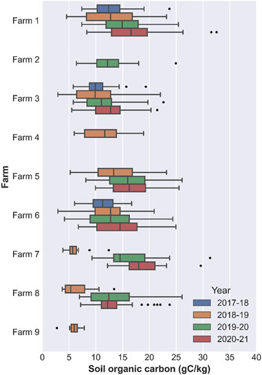
FIGURE 2. Boxplot of the soil organic carbon (SOC) content for the nine sampled farms in the four sampled production years.
Additionally, the mean SOC content was 13.12 g kg−1. The lowest observed SOC content was 4.70 g kg−1 (Farm 9 in 2018-19), and the maximum observed SOC content was 32.54 g kg−1 (Farm 1 in 2020-21). A positive correlation was observed between the number of samples per farm and the variation of SOC. Farm 1 was the farm with the highest variation of SOC. It had an interquartile distance (considering all years) of 8.30 g kg−1. Farm 1 was also the farm with the highest number of soil samples (237). On the other hand, Farm 9, which had the lowest number of samples (12 samples), had the lowest interquartile distance, only 1.14 g kg−1. From the nine sampled farms, only one (Farm 4) is in Spain, but it has similar SOC content distribution as the other Portuguese farms. The average SOC content in Farm 4 is 13.10 g kg−1 (min: 6.03 g kg−1; max: 19.40 g kg−1) and the average SOC in the Portuguese farms is 13.6 g kg−1 (min: 4.70 g kg−1; max: 32.54 g−kg−1).
Although two sampling methods (manual and mechanical) were used for sample collection, the observed SOC content between the two methods was very similar. Specifically, the samples collected within the same farm using both methods show a high level of similarity (less than 7% differences with no observable bias), with any observed differences likely attributable to the typical spatial variation within the farm.
The Spearman rank correlation between observed SOC content and the input variables ranged between −0.61 and 0.32 (Figure 3). The lowest correlation corresponded to the correlation between SOC content the auxiliary dummy variable for manual or mechanical soil sampling (−0.61) and the highest correlation of SOC content was with the year (0.32). Analyzing the average correlation in absolute value, per type of input (according to the “Type” column in Table 3), auxiliary variables had the highest correlation (mean: 0.34), followed by climatic variables (mean: 0.22), and by terrain variables (mean: 0.14); the remaining average correlations were lower than 0.10. Despite the low correlations, about 80% (40 out of 49 input variables) were significantly correlated with SOC content, 37 variables at a significance level of 5% and 3 variables at 10% significance level.
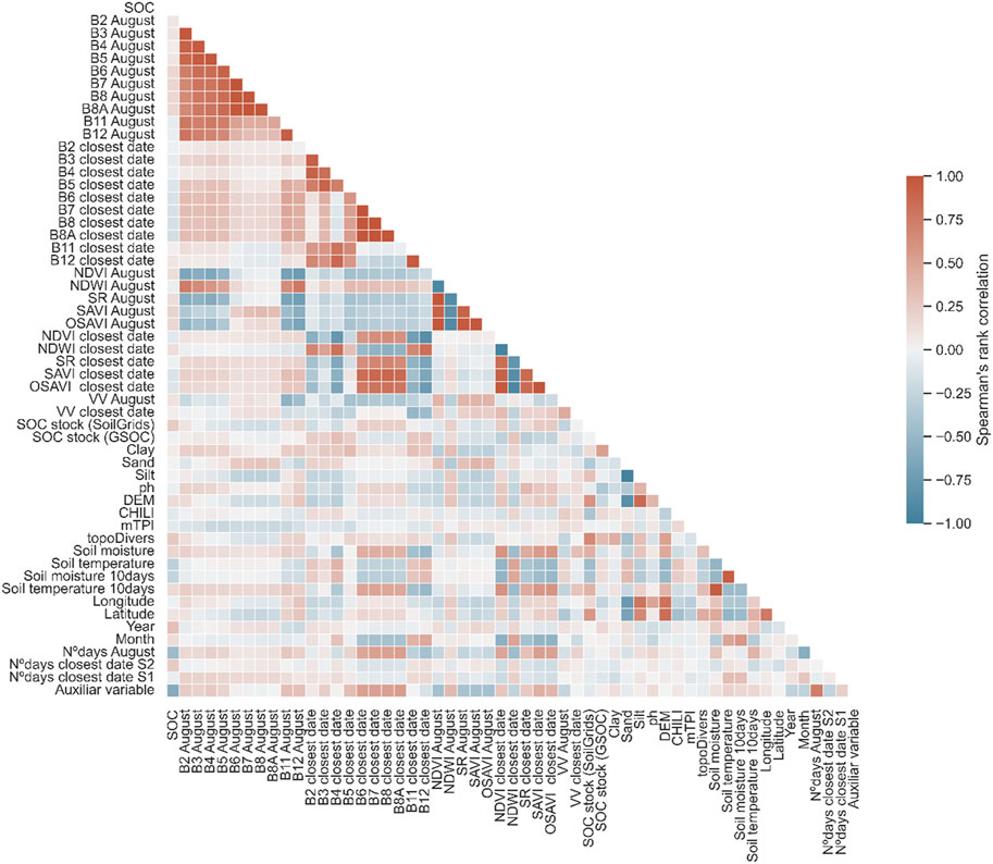
FIGURE 3. Spearman’s rank correlation between the soil organic carbon and the considered input variables. The input variables are: 22 individual bands from Sentinel-2 (11 in August and 11 in closest date), 2 individual bands from Sentinel-1 (1 in August and 1 in closest date), 10 vegetative indices (5 in August and 5 in closest date), SOC proxies, soil variables, terrain variables, auxiliar variables and location variables. Variable names are explained in Table 3.

TABLE 3. Description of the variables used to model soil organic carbon, including type of data, sources, variable and spatial resolution.
In the composite image of August, all bands were strongly and significantly correlated with each other (average correlation of 0.65); however, the correlation between bands in the Sentinel-2 image closest to the collection date was significantly lower (average correlation of 0.35). Vegetation indices, as expected, were strongly and significantly correlated with the Sentinel-2 imagery that was used to calculate them, i.e., vegetation indices in August are strongly correlated with the composite Sentinel-2 imagery. There were also strong correlations between location variables (latitude and longitude) and soil variables (sand, silt, and pH) and the DEM.
The feature selection procedure using SFS selected only 24 out of the 49 input variables considered in this work, representing approximately 48% of the total number of inputs. The selected inputs covered all the “Process Categories” defined in Table 2. The remote sensing imagery variables selected were Bands 2 and 12 from Sentinel-2 in August, Bands 3, 4, 7, 8, and 8 A from Sentinel-2 at the closest date, and VV from Sentinel-1 at the closest date. The vegetation indices selected were NDVI and NDWI in August, as well as NDVI, SR, SAVI, and OSAVI at the closest date. The selected climatic variable was soil temperature. The soil variables selected were silt content and pH. The terrain variables considered were the DEM and the mTPI. Additionally, the auxiliary variables selected were the number of days since August, the number of days from the closest Sentinel-2 imagery, and the month of the year. Lastly, both location variables, latitude and longitude, were also selected.
Among the regression methods used, XGB had the lowest estimation error for both feature selection approaches, as can be seen in Table 4 for the metrics of RMSE, rRMSE, RPD, and r2. A general trend is that more complex models (RF, XGB, and ANN) outperform simpler models (MLR) in predicting SOC content in SBP systems. When comparing the regression methods, the mean RMSE of XGB was, on average, 52% lower than the mean RMSE of the other methods in the training sets and 11% lower than the other methods in the test sets. Similar trends can be observed in the other estimation error metrics. For example, the difference between MLR (the method with the highest RMSE) and XGB was 72% in the training sets (MLR: 3.10 g kg−1; XGB: 0.87 g kg−1—considering the approach without feature selection), and the difference was 18% in the test sets (MLR: 3.27 g kg−1; XGB: 2.69 g kg−1). Further, decision tree methods (RF and XGB) have a lower estimation error than the other methods MLR, ANN). The RF and XGB regression methods had similar estimation errors in the test sets, but XGB performed better than RF in the training sets. MLR was also the regression method with the lowest variation of the RMSE between training and test sets, only 6% (considering the approach without feature selection). The estimation error between the training set and test set in the other methods always had an increase higher than 50%, e.g., for the ANN, the difference was about 56%. The XGB was the method with the highest error increase, considering the RMSE, it more than doubled in the test set in relation to the training set, but even so, it was lower than in other methods.
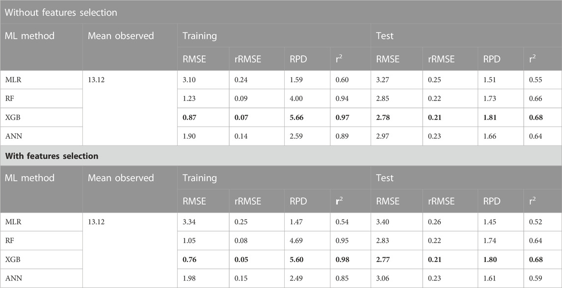
TABLE 4. Estimation accuracy of the soil organic carbon in the training and test set of the cross-validation approach, for all using each of the machine learning (ML) methods and for the two features selection approach. Metrics presented: considering mean root mean squared error (RMSE), relative RMSE (rRMSE), ratio of performance to deviation (RPD) and r squared (r2). MLR, Multiple linear regression; RF, Random forests; XGB, XGBoost; ANN, Artificial neural network. The model with the highest performance is in bold.
Using the feature selection approach, where only 24 out of the total 49 inputs were used, did not significantly influence the estimation error in the test sets for all regression methods. For example, considering XGB, the RMSE with feature selection was almost the same with all variables or with the selected variables (without selection: 2.78 g kg−1; with selection: 2.77 g kg−1). Nevertheless, in the training error, feature selection reduced the RMSE in RF and XGB (about 13%) and increased the RMSE of MLR and ANN (about 6%). This result highlights the efficacy of the feature selection approach in identifying the most relevant input variables for estimating SOC content. By accomplishing these dual objectives, the feature selection process enhances the convergence of the training procedure and ultimately improves the fitting performance of the RF and XGB models.
Considering XGB, there was no significant change in the estimation error between the two feature selection approaches. Figure 4 presents the estimated SOC versus the observed SOC when each sample is left on the test set using the approach with feature selection (using a hexagonal binning plot). As can be seen in Table 4, the estimation errors in the test sets were good, particularly in the region with the highest point density, i.e., between 10 and 15 g kg−1. In this region, the RMSE in the test sets decreased by about 20% (2.19 g kg−1). However, there was a non-significant overestimation of the observed SOC between 7 and 12 g kg−1. Additionally, there was a noticeable underestimation of the measured SOC in the highest values (higher than 20 g kg−1), which corresponds to the range of values with fewer observations.
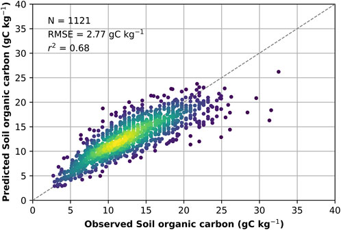
FIGURE 4. Estimated versus observed soil organic carbon (SOC) using the best model (XGBoost) in the features selection approach (i.e., only using 24 features).
In the XGB model with SFS, the VV feature (from Sentinel-1) had the highest importance (about 35%) in the obtained results. It was followed by the month of the year, latitude, and longitude. The Sentinel-2 bands in August (Bands 2 and 12) had the lowest contribution to the estimated SOC (less than 2%). Vegetation indices also had a greater relevance for SOC estimation than the individual satellite bands (each Vegetation Index at the closest date has a feature relevance of about 5%, and individual bands are lower than 3%). The terrain variables with the highest contribution are DEM and mTPI with an importance of 3% and 4%, respectively. All the soil input data has an accumulated importance lower than 7%.
The obtained models can be used to estimate SOC for entire parcels in the farms. As an example of the application, Figure 5 depicts the spatial representation of SOC in the 9 sampled farms. This figure was obtained for the day of 29 May 2021, using the dynamic input data for that day, namely, the climatic data, Sentinel-2 imagery, and vegetation indices. Sentinel-1 imagery was not available for the same date, so we used Sentinel-1 imagery for the closest date, i.e., 27 May 2021. All the other input data is static, so it was not influenced by the date. The model used was the XGB model with the feature selection approach.
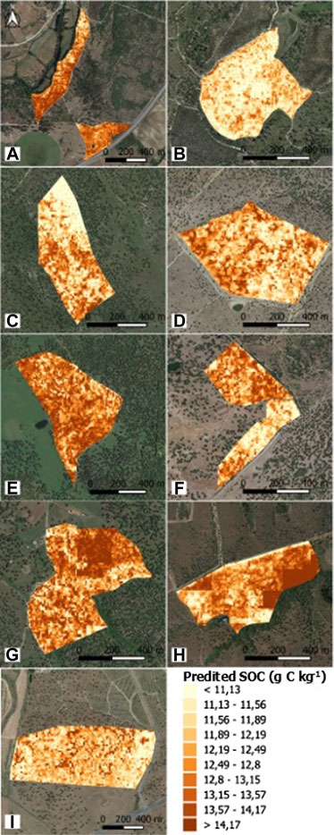
FIGURE 5. Spatial representation of the predicted SOC in the 9 sampled farms using the best model (XGBoost) in the features selection approach (i.e., only using 12 inputs). These results were obtained using the Sentinel-2 image of May 29 and Sentinel-1 image of 27 May 2021. (A) Farm 1; (B) Farm 2; (C) Farm 3; (D) Farm 4; (E) Farm 5; (F) Farm 6; (G) Farm 7; (H) Farm 8; (I) Farm 9.
The trends observed in SOC between farms in Figure 2 are also verified when the XGB model was applied to the entire farm. For example, Farms 1, 5, and 7 had the highest mean SOC in the year 2020–2021 in both observed and predicted values. Farm 8 was the farm with the highest spatial variation (standard deviation (SD) of 1.34 g kg−1) and Farm 2 had the lowest spatial variation (SD: 0.74 g kg−1). The minimum predicted SOC was also in Farm 2 (7.56 g kg−1) and the highest predicted SOC was in Farm 8 (18.80 g kg−1). Farm 2 had the lowest predicted SOC, 7.56 g kg−1, but this farm was not sampled in the production year 2020-2021. However, there are other aspects that vary from the observed data. For example, in the observed date, in the production year of 2020-2021, Farm 1 has the highest SOC (32.54 g kg−1) and the highest predicted SOC was at Farm 8, 18.80 g kg−1 in the predicted results. Nevertheless, the highest observed SOC at Farm 1 was in January (on January 16), which is significantly far from the date of May 29. Between January and May, soil temperature increases and soil moisture decreases, which supports SOC mineralization.
This study demonstrated that more complex models (such as RF, XGB, and ANN) perform better in predicting SOC content in SBP systems in Portugal and Spain compared to simpler models like MLR (Liu et al., 2011; Ali et al., 2016). Complex models are capable of capturing complex, high-dimensional relationships between dependent and explanatory variables, which simple models cannot achieve. Two feature selection approaches were used to evaluate the performance impact. Our findings indicate that using all 49 input variables or a subset of just 24 (48%) yields comparable estimation performance in both training and testing phases. Moreover, the remaining variables encompassed almost all data categories that affect SOC content, including remote sensing, climatic, soil, and terrain characteristics.
Over the last decade, there has been a substantial increase in the number of combined applications that utilize satellite RS and ML to estimate SOC or SOM content. To investigate the extent of this increase, we conducted a very simple search in the Google Scholar database on 10 January 2023, specifically focusing on papers that estimated SOC content in pastures or grasslands using satellite RS. We utilized the search string: “(soil organic matter” OR “soil organic carbon”) AND “remote sensing” AND “satellite” AND “regression” AND “machine learning” AND (“grassland” OR “pasture”), which resulted in 2,110 hits. Of these, 30% (688 hits) were from 2022 to 50% (1,080 hits) were from 2021. However, upon sorting the results by relevance according to Google Scholar, none of the first 50 hits were focused on grassland or pasture systems as the present paper does. This analysis is by no means a thorough review of the literature and surely depicts incomplete results, but shows that grassland systems remain under analysed and, in particular, this is the first study of this nature focusing on SBP.
This paper achieved better estimation performance for SOC content in grasslands and pastures compared to many other papers in the literature. For instance, Zhou et al. (2021) obtained an r2 of 0.47 in their best model using a cross-validation approach for Switzerland’s multiple land use/cover systems, whereas the highest r2 obtained in this study was 0.70. Hamzehpour et al. (2019) predicted SOC stock in a sub-region of Iran and achieved an r2 of 0.44, while Wu et al. (2019) predicted SOC content in a sub-region of China using various machine learning regression models, and their best model, XGB, had an r2 of 0.74, which was similar to the r2 obtained in this paper. Similarly, Keskin et al. (2019) estimated total soil carbon in a sub-region of the United States of America using multiple regression models, and the best model was a RF with an r2 of 0.72 in the validation set. Notably, decision trees consistently outperformed other simpler or more complex methods (such as ANNs) in all the studies that used different regression methods. In this study, extreme gradient boosting (XGB) demonstrated superior performance compared to the other models. Specifically, the XGB model, along with other decision tree-based models, outperformed artificial neural networks (ANN). There are several plausible reasons for this observation. Firstly, XGB models tend to be less reliant on extensive fine-tuning of hyperparameters, potentially contributing to their improved performance, as suggested by the results (Memon et al., 2019; Shwartz-Ziv and Armon, 2022).
In this study, we observed that the estimation accuracy for the highest SOC values was significantly lower than that for low-medium values. This trend has been observed in other studies that estimated SOC, as well as in the estimation of other variables in croplands and grasslands, among others (Castaldi et al., 2018). The normal frequency distribution of the data on SOC is the cause of this limitation since the dataset is dominated by mid-range values. To overcome this limitation, quantile regression methods based on the approach used in this study can be employed, such as quantile RF. Quantile regression models the relationship between independent variables and specific percentiles of the dependent variable, which is an improvement over regression methods that represent the mean increase in the response function produced by one unit increase in the associated independent variables. In fact, recent studies have applied these regression methods to SOC estimation (Lombardo et al., 2018; Kasraei et al., 2021; Zhao et al., 2021). In the future, the application of these methods should be tested to confirm if the estimation performance increases significantly.
In addition, the number of observations per farm can also influence results. It has been observed that the model tends to achieve a better fit when applied to farms with a larger number of samples compared to those with a smaller number of samples. For instance, Farm 1 consists of a total of 237 samples, while Farm 2 comprises only 35 samples. Consequently, the model is more likely to exhibit improved performance in capturing the specific characteristics associated with Farm 1 rather than Farm 2. The imbalance in the number of observations across farms may also impact the generalization error when applying the model to other locations. However, considering that the characteristics of the different farms are not significantly different, we do not anticipate that the obtained model would yield highly inaccurate estimations of SOC content for the sample used here. The effectiveness of the model when applied to other SBP farms should be assessed in future research work.
Here, we developed a rapid and cost-effective indirect method for the purpose of expedite mapping of SOC in SBP farms. This represents a significant improvement compared to the approach proposed by Morais et al. (2021), which relied on data from in situ field spectrometry and only replaced the laboratory analysis. In terms of results, the obtained r2 value (0.68) is lower than the value previously reported by Morais et al. (0.80). However, it is important to note that our method is solely based on remote sensing data and therefore applicable to multiple farms and regions without the need for repeated field work and laboratory analysis.
In this study, we used RS data from Sentinel-1 and Sentinel-2, which offer significantly higher spatial resolution compared to other spatially explicit variables. The inclusion of Sentinel-1 and Sentinel-2 data allowed us to capture fine-scale spatial variations within individual parcels or farms. Conversely, other static data sources with lower spatial resolution lacking the capability to capture intricate spatial variations within parcels primarily facilitated the assessment of regional variation. Additionally, remote sensing data provided a distinct advantage by enabling us to capture of temporal variations across different years, as they were the only data sources exhibiting temporal variability over time. Despite achieving good performance in our study, there is potential for improvement by enhancing the quality of climatic and soil data. It is important to note that the SFS method, while not affecting SOC estimation performance, may be influenced by the spatial resolution of the input data. SFS excluded soil temperature and soil moisture as explanatory variables, probably due to the course scale of the data sources available. However, those variables are vital in regulating microbial activity, nutrient availability, and overall soil health. The same was true of some climate variables, which had a spatial resolution of 27 km, which may be insufficient for depicting intra-farm variations.
RS data derived from Sentinel-1 and Sentinel-2 present a significantly elevated spatial resolution in comparison to other spatially explicit variables. The utilization of Sentinel-1 and Sentinel-2 data enables the capture of intricate spatial variations within individual parcels or farms. Conversely, static data sources with diminished spatial resolution predominantly facilitate the assessment of regional variations, as they lack the ability to capture the detailed spatial nuances within parcels. Moreover, remote sensing data proffers the distinct advantage of capturing temporal variations across different years, rendering it the sole data source characterized by temporal variability over time. In fact, this procedure of using multiple data sources with multiple spatial and temporal resolutions is frequently used to characterize different land cover systems (Zhang et al., 2016; Venter and Sydenham, 2021), namely, to estimate SOC content, e.g., Venter et al. (2021). Nevertheless, enhancing the spatial resolution of the data with low spatial resolution could potentially improve the estimation performance of SOC content. For example, in this study, the soil data used had a spatial resolution of 250 m. It is not expected that soil characteristics such as sand, clay, and silt fractions would vary significantly within the same farm. Consequently, the variables that contributed the most to explaining SOC content were the ones that had the higher resolutions, such as those measured or calculated from Sentinel-1 and Sentinel-2 data. Increasing the spatial resolution of coarse soil-specific data could enhance the fine variation of SOC content and help address some of the variance unexplained by our model.
The obtained models in this study have a spatial resolution of 10 m, which is the lowest resolution among all the spatialized data used, including Sentinel-1 data and the red, green, and blue bands of Sentinel-2. However, even this resolution may not be sufficient to capture all the spatial variability of pasture systems such as SBP. To enhance the spatial resolution of RS data from satellites, UAVs can be utilized. UAVs can have a spatial resolution of a few centimeters, providing a significant improvement in spatial resolution. For instance, a 5 cm resolution UAV would yield 100,000 pixels in a 10 × 10 m pixel of Sentinel-2. UAVs are currently preferred for agricultural land characterization due to their affordability and ease of operation. Nonetheless, UAV data has a significantly lower spatial coverage, lower spectral resolution, and potentially lower temporal coverage than satellite data (Colomina and Molina, 2014; Vilar et al., 2020). Moreover, the quality of UAV data can be negatively impacted by factors such as sun elevation angle, diffuse sunlight, and shadow effects of objects such as trees (De Luca et al., 2019). Rather than completely replacing satellite data with UAV data, it is more beneficial to use them in combination to minimize estimation errors. For instance, Maimaitijiang et al. (2020) improved the estimation of biomass characteristics by integrating RGB UAV data with Sentinel-2 data.
In this paper, we used individual bands from the Sentinel-1 satellite. Nevertheless, recent research has proposed a technique to merge two Sentinel-1 image products of complementary polarimetric information (HH/HV and VH/VV) to derive pseudo-polarimetric features (Braun and Offermann, 2022). Despite some inaccuracies, the polarimetric features turned out to improve potential land cover mapping compared with backscatter intensities and dual-polarization features of the input products alone. However, such a technique has not yet been tested in regression problems to estimate SOC content. Alternatively, synthetic-aperture radar data from other satellites could provide different bands and wavelengths (Moreira et al., 2013). Data with different wavelengths and frequencies also have different penetration power, spatial resolution, sensitivity to surface roughness, and sensitivity to atmospheric effects (Moreira et al., 2013; Paek et al., 2020; Le et al., 2021). The C-band used in Sentinel-1 refers to the microwave frequency range between 4 to 8 GHz (Gigahertz) in the electromagnetic spectrum (ESA, 2022). It is one of the most commonly used bands in SAR remote sensing due to its favourable characteristics, namely: moderate penetration capabilities, meaning it can penetrate through vegetation and light to moderate rainfall; good spatial resolution allowing the detection of small to medium-sized features on the Earth’s surface; sensitivity to surface roughness variations, which makes it useful for monitoring changes in ocean waves, soil moisture, and snow cover; and is less affected by atmospheric conditions like clouds and precipitation compared to higher-frequency bands (e.g., X-band or Ku-band) (Monti-Guarnieri et al., 2017; ESA, 2022). Another frequency band that is commonly used is the P band, for example, used in ALOS (Advanced Land Observing Satellite) PALSAR (Phased Array type L-band Synthetic Aperture Radar), which is in the microwave frequency range between 0.3 to 1 GHz (Gigahertz) in the electromagnetic spectrum. The P-band has higher penetration than the C-band. Due to its lower frequency, P-band SAR typically has a coarser spatial resolution compared to higher-frequency bands like the C-band. P-band SAR is also less sensitive to surface roughness compared to C-band SAR, but it is relatively less affected by atmospheric conditions (Li et al., 2019; Minh et al., 2021). Other bands with higher frequency (e.g., X-band) have higher spatial resolution but lower penetration capacity (Zhou et al., 2020). Thus, in the future, approaches that combine alternative/complementary SAR data should be tested to improve the characterization of land cover systems, such as grasslands.
Here we used several vegetation indices (NDVI, NDWI, SR, SAVI, and OSAVI) as well as the raw data for the bands used to calculate them. The fact that the bands are used nonlinearly takes away some of the explanatory power of the indices. However, because the indices were more important than the individual bands in our results, exploring additional indices may offer valuable insights into SOC content estimation. For example, the Normalized Difference Red/Green Redness Index and the Dark Green Color Index that utilize both red and green bands have been previously used to estimate SOC content in agricultural soils (Heil et al., 2022). These and other alternative indices could potentially complement the existing ones and enhance the accuracy of SOC estimation.
In this study, we did not perform an assessment of bare soil pixels, which is a common practice in other research studies (Bhunia et al., 2017; Castaldi, 2021). Typically, bare soil pixels are determined using vegetation indices calculated from individual bands of Sentinel-2, such as NDVI and normalized burn ratio 2 (NBR2) (Castaldi, 2021). This process involves defining a threshold for the vegetation indices, and pixels with lower values than the threshold are classified as bare. However, the number of bare soil pixels can vary significantly depending on the chosen thresholds. For instance, Castaldi (2021) observed that reducing the NBR2 threshold from 0.2 to 0.05 in Northeastern Germany croplands led to a decrease in the percentage of Sentinel-2 pixels classified as bare soil from over 25% to about 10%. Additionally, this method requires the removal of data points that do not meet the defined thresholds. For these reasons, we chose not to use this approach. Instead, we utilized data not only near the sampling date but also data from August when the soil is mostly bare in well-managed SBP systems. Incorporating observations from August allows us to capture the soil’s characteristics when it is bare, while observations near the sampling date enable us to indirectly evaluate the effect of vegetation on SOC.
The models that we developed lack a formal representation of the processes that occur in soil and influence SOC content, such as an equation for SOC mineralization that process-based models possess (Morais et al., 2019). Unlike data-driven models, process-based soil models consider biogeochemical processes formulated based on mathematical-ecological theory (Coleman et al., 1997; Liu et al., 2011). These models’ equations are often derived from statistical relationships, which can be improved by incorporating data-driven modeling approaches. Combining the benefits of both data-driven models (such as those used in this study) and process-based modeling is critical for developing more robust models in the future. One approach is to replace process-based models’ rate modifiers with ML models. Tsai et al. (2021) have done this successfully to predict soil moisture and streamflow.
The models derived in this study have the potential to retrospectively estimate SOC content since 2015 when Sentinel-2 data was initiated. Consequently, a considerable amount of data can be generated that can be employed in other models. Process-based models, such as those that evaluate soil sinks and emissions of carbon and nitrogen and their impacts on environmental concerns, can benefit significantly from longer data series (Prado et al., 2006; Morais et al., 2018; Teixeira et al., 2019).
This work combined multiple data types from different sources with ML methods in order to estimate SOC content of SBP in Portugal and Spain. The most relevant variables that are known to influence SOC content and change, such as climatic, soil, and terrain characteristics, were combined with RS imagery. The most relevant variables from the full set of independent (or input) data were selected using an SFS approach. This approach reduced the number of variables to 24 (instead of 49) but maintained the overall accuracy of the best model: without feature selection, the root mean squared error (RMSE) was 2.78 g kg-1 (on the test set) and with feature selection, the RMSE was 2.77 g kg-1. XGB was the model with the highest estimation performance, using a cross-validation approach.
SOC content plays a significant role in plant growth and characteristics. Nevertheless, the type of models developed in this work are still infrequently used as a farm management tool, despite the fact that they are powerful tools that could increase incomes and/or reduce costs. Based on the best models, SOC content can be approximately estimated throughout the year, even when the soil is covered by plants, and with that, advisors can inform farmers to perform practices to improve soil quality for plant and animal production.
The raw data supporting the conclusion of this article will be made available by the authors, without undue reservation.
TM, TD, and RT contributed to the conceptualization and methodology of the study. MJ, CM, NR, IG, and JS performed field investigations. MG and RM were responsible for lab analysis of the soil samples. TM, TD, and RT contributed to data analysis and interpretation of the results. All authors contributed to the article and approved the submitted version.
This work was supported by Fundação para a Ciência e Tecnologia through projects “GrassData—Development of algorithms for identification, monitoring, compliance checks and quantification of carbon sequestration in pastures” (DSAIPA/DS/0074/2019), “LEAnMeat—Lifecycle-based Environmental Assessment and impact reduction of Meat production with a novel multi-level tool” (PTDC/EAM-AMB/30809/2017), and CEECIND/00365/2018 (RT). This work was also supported by FCT/MCTES (PIDDAC) through project LARSyS—FCT Pluriannual funding 2020-2023 (UIDP/EEA/50009/2020), by COMPETE 2020, FEDER through project GreenBeef– “GreenBeef: Towards carbon neutral Angus beef production in Portugal “(POCI-01-0247-FEDER-047050) and by Programa de desenlvolvimento rural (PDR 2020) through “GO SOLO: Avaliação da dinâmica da matéria orgânica em solos de pastagens semeadas biodiversas através do desenvolvimento de um método de monitorização expedito e a baixo custo” (PDR2020-101-031243).
The authors declare that the research was conducted in the absence of any commercial or financial relationships that could be construed as a potential conflict of interest.
All claims expressed in this article are solely those of the authors and do not necessarily represent those of their affiliated organizations, or those of the publisher, the editors and the reviewers. Any product that may be evaluated in this article, or claim that may be made by its manufacturer, is not guaranteed or endorsed by the publisher.
Ali, I., Cawkwell, F., Dwyer, E., Barrett, B., and Green, S. (2016). Satellite remote sensing of grasslands: from observation to management. J. Plant Ecol. 9, 649–671. doi:10.1093/jpe/rtw005
Angelopoulou, T., Tziolas, N., Balafoutis, A., Zalidis, G., and Bochtis, D. (2019). Remote sensing techniques for soil organic carbon estimation: A review. Remote Sens. 11, 676. doi:10.3390/rs11060676
APA (2018). Portuguese national inventory report on greenhouse gases, 1990 - 2018. Amadora, Portugal: Portuguese Environmental Agency.
Bardgett, R. D., Bullock, J. M., Lavorel, S., Manning, P., Schaffner, U., Ostle, N., et al. (2021). Combatting global grassland degradation. Nat. Rev. Earth Environ. 2, 720–735. doi:10.1038/s43017-021-00207-2
Bhunia, G. S., Kumar Shit, P., and Pourghasemi, H. R. (2017). Soil organic carbon mapping using remote sensing techniques and multivariate regression model. Geocarto Int. 1, 215–226. doi:10.1080/10106049.2017.1381179
Biney, J. K. M. (2022). Verifying the predictive performance for soil organic carbon when employing field Vis-NIR spectroscopy and satellite imagery obtained using two different sampling methods. Comput. Electron. Agric. 194, 106796. doi:10.1016/J.COMPAG.2022.106796
Braun, A., and Offermann, E. (2022). Polarimetric information content of Sentinel-1 for land cover mapping: an experimental case study using quad-pol data synthesized from complementary repeat-pass acquisitions. Front. Remote Sens. 3. doi:10.3389/frsen.2022.905713
Castaldi, F., Chabrillat, S., Jones, A., Vreys, K., Bomans, B., and van Wesemael, B. (2018). Soil organic carbon estimation in croplands by hyperspectral remote APEX data using the LUCAS topsoil database. Remote Sens. 10, 153. doi:10.3390/rs10020153
Castaldi, F. (2021). Sentinel-2 and landsat-8 multi-temporal series to estimate topsoil properties on croplands. Remote Sens. 13, 3345. doi:10.3390/RS13173345
Chan, C. K., Gomez, C. A., Kothikar, A., and Baiz-Villafranca, P. M. (2023). Satellite-based carbon estimation in scotland: AGB and SOC. Land 12, 818. doi:10.3390/land12040818
Chappell, A., Baldock, J., and Sanderman, J. (2016). The global significance of omitting soil erosion from soil organic carbon cycling schemes. Nat. Clim. Chang. 6, 187–191. doi:10.1038/nclimate2829
Chen, T., and Guestrin, C. (2016). “XGBoost: A scalable tree boosting system,” in Proceedings of the ACM SIGKDD International Conference on Knowledge Discovery and Data Mining, San Francisco California USA, August 2016. doi:10.1145/2939672.2939785
Coleman, K., Jenkinson, D. S., Crocker, G. J., Grace, P. R., Klír, J., Körschens, M., et al. (1997). Simulating trends in soil organic carbon in long-term experiments using RothC-26.3. Geoderma 81, 29–44. doi:10.1016/S0016-7061(97)00079-7
Colomina, I., and Molina, P. (2014). Unmanned aerial systems for photogrammetry and remote sensing: A review. ISPRS J. Photogramm. Remote Sens. 92, 79–97. doi:10.1016/j.isprsjprs.2014.02.013
Davids, C., Karlsen, S. R., Ancin, M., and Jorgensen, M. (2018). “UAV based mapping of grassland yields for forage production in northern Europe Sustainable meat and milk production from grasslands,” in Proceedings of the 27th General Meeting of the European Grassland Federation, Cork, Ireland, June 2018, 845–847.
De Luca, G., Silva, N. J. M., Cerasoli, S., Araújo, J., Campos, J., et al. (2019). Object-based land cover classification of cork oak woodlands using UAV imagery and orfeo ToolBox. Remote Sens. 11, 1238. doi:10.3390/rs11101238
Doetterl, S., Stevens, A., Six, J., Merckx, R., Van Oost, K., Casanova Pinto, M., et al. (2015). Soil carbon storage controlled by interactions between geochemistry and climate. Nat. Geosci. 8, 780–783. doi:10.1038/ngeo2516
Egoh, B. N., Bengtsson, J., Lindborg, R., Bullock, J. M., Dixon, A. P., Rouget, M., et al. (2016). “The importance of grasslands in providing ecosystem services,” in Routledge handbook of ecosystem services (New York, NY: Routledge), 421–441. doi:10.4324/9781315775302-37
ESA (2022). Sentinel-1 - missions - Sentinel online - Sentinel online. Eur. Sp. Agency. Available at: https://sentinel.esa.int/web/sentinel/missions/sentinel-1 (Accessed June 26, 2023).
ESDAC (2003). European Soil Database (distribution version v2.0). Brussels (Belgium): European Commission Joint Research Centre.
Gao, B. C. (1996). Ndwi - a normalized difference water index for remote sensing of vegetation liquid water from space. Remote Sens. Environ. 58, 257–266. doi:10.1016/S0034-4257(96)00067-3
Gardin, L., Chiesi, M., Fibbi, L., and Maselli, F. (2021). Mapping soil organic carbon in Tuscany through the statistical combination of ground observations with ancillary and remote sensing data. Geoderma 404, 115386. doi:10.1016/j.geoderma.2021.115386
Giardina, C. P., Litton, C. M., Crow, S. E., and Asner, G. P. (2014). Warming-related increases in soil CO2 efflux are explained by increased below-ground carbon flux. Nat. Clim. Chang. 4, 822–827. doi:10.1038/nclimate2322
Goodfellow, I., Bengio, Y., and Courville, A. (2016). Deep learning (adaptive computation and machine learning series). Cambridge, England: MIT Press.
Hamzehpour, N., Shafizadeh-Moghadam, H., and Valavi, R. (2019). Exploring the driving forces and digital mapping of soil organic carbon using remote sensing and soil texture. CATENA 182, 104141. doi:10.1016/J.CATENA.2019.104141
Heil, J., Jörges, C., and Stumpe, B. (2022). Fine-scale mapping of soil organic matter in agricultural soils using UAVs and machine learning. Remote Sens. 14, 3349. doi:10.3390/rs14143349
Hengl, T., Mendes de Jesus, J., Heuvelink, G. B. M., Ruiperez Gonzalez, M., Kilibarda, M., Blagotić, A., et al. (2017). SoilGrids250m: global gridded soil information based on machine learning. PLoS One 12, e0169748. doi:10.1371/journal.pone.0169748
Huete, A. R. (1988). A soil-adjusted vegetation index (SAVI). Remote Sens. Environ. 25, 295–309. doi:10.1016/0034-4257(88)90106-X
IPMA (2018). Climate normals. Available at: http://www.ipma.pt/en/index.html (Accessed January 18, 2018).
Jobbágy, E. G., and Jackson, R. B. (2000). The vertical distribution of soil organic carbon and its relation to climate and vegetation. Ecol. Appl. 10, 423–436. doi:10.1890/1051-0761(2000)010[0423:TVDOSO]2.0.CO;2
Kasraei, B., Heung, B., Saurette, D. D., Schmidt, M. G., Bulmer, C. E., and Bethel, W. (2021). Quantile regression as a generic approach for estimating uncertainty of digital soil maps produced from machine-learning. Environ. Model. Softw. 144, 105139. doi:10.1016/J.ENVSOFT.2021.105139
Keskin, H., Grunwald, S., and Harris, W. G. (2019). Digital mapping of soil carbon fractions with machine learning. Geoderma 339, 40–58. doi:10.1016/J.GEODERMA.2018.12.037
Koven, C. D., Hugelius, G., Lawrence, D. M., and Wieder, W. R. (2017). Higher climatological temperature sensitivity of soil carbon in cold than warm climates. Nat. Clim. Chang. 7, 817–822. doi:10.1038/nclimate3421
Ladoni, M., Bahrami, H. A., Alavipanah, S. K., and Norouzi, A. A. (2010). Estimating soil organic carbon from soil reflectance: A review. Precis. Agric. 11, 82–99. doi:10.1007/s11119-009-9123-3
Lamichhane, S., Kumar, L., and Wilson, B. (2019). Digital soil mapping algorithms and covariates for soil organic carbon mapping and their implications: A review. Geoderma 352, 395–413. doi:10.1016/j.geoderma.2019.05.031
Le, N. N., Pham, T. D., Yokoya, N., Ha, N. T., Nguyen, T. T. T., Tran, T. D. T., et al. (2021). Learning from multimodal and multisensor earth observation dataset for improving estimates of mangrove soil organic carbon in Vietnam. Int. J. Remote Sens. 42, 6866–6890. doi:10.1080/01431161.2021.1945158
Li, W., Tong, Q., Xu, L., Ji, P., Dong, F., Yu, Y., et al. (2019). “The P-band SAR satellite: opportunities and challenges,” in Proceedings of the 2019 6th Asia-Pacific Conf. Synth. Aperture Radar, (APSAR), Xiamen, China, November 2019. doi:10.1109/APSAR46974.2019.9048581
Liu, D. L., Chan, K. Y., Conyers, M. K., Li, G., and Poile, G. J. (2011). Simulation of soil organic carbon dynamics under different pasture managements using the RothC carbon model. Geoderma 165, 69–77. doi:10.1016/j.geoderma.2011.07.005
Lombardo, L., Saia, S., Schillaci, C., Mai, P. M., and Huser, R. (2018). Modeling soil organic carbon with Quantile Regression: dissecting predictors’ effects on carbon stocks. Geoderma 318, 148–159. doi:10.1016/J.GEODERMA.2017.12.011
Maimaitijiang, M., Sagan, V., Sidike, P., Daloye, A. M., Erkbol, H., and Fritschi, F. B. (2020). Crop monitoring using satellite/UAV data fusion and machine learning. Remote Sens. 12, 1357. doi:10.3390/RS12091357
Mallik, S., Bhowmik, T., Mishra, U., and Paul, N. (2020). Mapping and prediction of soil organic carbon by an advanced geostatistical technique using remote sensing and terrain data. Geocarto Int. 37, 2198–2214. doi:10.1080/10106049.2020.1815864
Mariano, D. A., Santos, C. A. C. dos, Wardlow, B. D., Anderson, M. C., Schiltmeyer, A. V., Tadesse, T., et al. (2018). Use of remote sensing indicators to assess effects of drought and human-induced land degradation on ecosystem health in Northeastern Brazil. Remote Sens. Environ. 213, 129–143. doi:10.1016/J.RSE.2018.04.048
Memon, N., Patel, S. B., and Patel, D. P. (2019). “Comparative analysis of artificial neural network and XGBoost algorithm for PolSAR image classification,” in Lecture notes in computer science (including subseries lecture notes in artificial intelligence and lecture notes in bioinformatics (Berlin, Germany: Springer). doi:10.1007/978-3-030-34869-4_49
Minh, D. H. T., Ngo, Y. N., and Lê, T. T. (2021). Potential of P-band SAR tomography in forest type classification. Remote Sens. 13, 696. doi:10.3390/RS13040696
Monti-Guarnieri, A., Giudici, D., and Recchia, A. (2017). Identification of C-band radio frequency interferences from sentinel-1 data. Remote Sens. 9, 1183. doi:10.3390/RS9111183
Morais, T. G., Jongen, M., Tufik, C., Rodrigues, N. R., Gama, I., Fangueiro, D., et al. (2022). Characterization of Portuguese sown rainfed grasslands using remote sensing and machine learning. Precis. Agric. 24, 161–186. doi:10.1007/s11119-022-09937-9
Morais, T. G., Teixeira, R. F. M., and Domingos, T. (2019). Some croplands can potentially accumulate more soil carbon than forests and grasslands: implications of detailed global modelling. PLoS One 14, e0222604. doi:10.1371/journal.pone.0222604
Morais, T. G., Teixeira, R. F. M., Rodrigues, N. R., and Domingos, T. (2018). Characterizing livestock production in Portuguese sown rainfed grasslands: applying the inverse approach to a process-based model. Sustainability 10, 4437. doi:10.3390/su10124437
Morais, T. G., Tufik, C., Rato, A. E., Rodrigues, N. R., Gama, I., Jongen, M., et al. (2021). Estimating soil organic carbon of sown biodiverse permanent pastures in Portugal using near infrared spectral data and artificial neural networks. Geoderma 404, 115387. doi:10.1016/J.GEODERMA.2021.115387
Moreira, A., Prats-Iraola, P., Younis, M., Krieger, G., Hajnsek, I., and Papathanassiou, K. P. (2013). A tutorial on synthetic aperture radar. IEEE Geosci. Remote Sens. Mag. 1, 6–43. doi:10.1109/MGRS.2013.2248301
Moreno, G., Hernández-Esteban, A., Rolo, V., and Igual, J. M. (2021). The enduring effects of sowing legume-rich mixtures on the soil microbial community and soil carbon in semi-arid wood pastures. Plant Soil 465, 563–582. doi:10.1007/s11104-021-05023-7
Odebiri, O., Odindi, J., and Mutanga, O. (2021). Basic and deep learning models in remote sensing of soil organic carbon estimation: A brief review. Int. J. Appl. Earth Obs. Geoinf. 102, 102389. doi:10.1016/j.jag.2021.102389
Orgiazzi, A., Ballabio, C., Panagos, P., Jones, A., and Fernández-Ugalde, O. (2018). LUCAS soil, the largest expandable soil dataset for europe: A review. Eur. J. Soil Sci. 69, 140–153. doi:10.1111/EJSS.12499
Paek, S. W., Balasubramanian, S., Kim, S., and de Weck, O. (2020). Small-satellite synthetic aperture radar for continuous global biospheric monitoring: A review. Remote Sens. 12, 2546. doi:10.3390/RS12162546
Pan, Y., Zhang, X., Liu, H., Wu, D., Dou, X., Xu, M., et al. (2022). Remote sensing inversion of soil organic matter by using the subregion method at the field scale. Precis. Agric. 23, 1813–1835. doi:10.1007/s11119-022-09914-2
Pezzuolo, A., Dumont, B., Sartori, L., Marinello, F., De Antoni Migliorati, M., and Basso, B. (2017). Evaluating the impact of soil conservation measures on soil organic carbon at the farm scale. Comput. Electron. Agric. 135, 175–182. doi:10.1016/J.COMPAG.2017.02.004
Pouladi, N., Møller, A. B., Tabatabai, S., and Greve, M. H. (2019). Mapping soil organic matter contents at field level with Cubist, Random Forest and kriging. Geoderma 342, 85–92. doi:10.1016/j.geoderma.2019.02.019
Prado, A. d., Brown, L., Schulte, R., Ryan, M., and Scholefield, D. (2006). Principles of development of a mass balance N cycle model for temperate grasslands: an Irish case study. Nutr. Cycl. Agroecosyst. 74, 115–131. doi:10.1007/s10705-005-5769-z
Rey, A., Petsikos, C., Jarvis, P. G., and Grace, J. (2005). Effect of temperature and moisture on rates of carbon mineralization in a Mediterranean oak forest soil under controlled and field conditions. Eur. J. Soil Sci. 56, 589–599. doi:10.1111/j.1365-2389.2004.00699.x
Rodell, M., Houser, P. R., Jambor, U., Gottschalck, J., Mitchell, K., Meng, C. J., et al. (2004). The global land data assimilation system. Bull. Am. Meteorol. Soc. 85, 381–394. doi:10.1175/BAMS-85-3-381
Rogge, D., Bauer, A., Zeidler, J., Mueller, A., Esch, T., and Heiden, U. (2018). Building an exposed soil composite processor (SCMaP) for mapping spatial and temporal characteristics of soils with Landsat imagery (1984–2014). Remote Sens. Environ. 205, 1–17. doi:10.1016/j.rse.2017.11.004
Rondeaux, G., Steven, M., and Baret, F. (1996). Optimization of soil-adjusted vegetation indices. Remote Sens. Environ. 55, 95–107. doi:10.1016/0034-4257(95)00186-7
Rubel, F., and Kottek, M. (2010). Observed and projected climate shifts 1901-2100 depicted by world maps of the Köppen-Geiger climate classification. Meteorol. Z. 19, 135–141. doi:10.1127/0941-2948/2010/0430
Rumelhart, D. E., Hinton, G. E., and Williams, R. J. (1986). Learning representations by back-propagating errors. Nature 323, 533–536. doi:10.1038/323533a0
Shwartz-Ziv, R., and Armon, A. (2022). Tabular data: deep learning is not all you need. Inf. Fusion 81, 84–90. doi:10.1016/j.inffus.2021.11.011
Spearman, C. (1904). The proof and measurement of association between two things. Am. J. Psychol. 15, 72–101. doi:10.2307/1412159
Sun, S., Zuo, Z., Yue, W., Morel, J., Parsons, D., Liu, J., et al. (2021). Estimation of biomass and nutritive value of grass and clover mixtures by analyzing spectral and crop height data using chemometric methods. Comput. Electron. Agric. 192, 106571. doi:10.1016/J.COMPAG.2021.106571
Teixeira, R. F. M., Barão, L., Morais, T. G., and Domingos, T. (2019). BalSim: A carbon, nitrogen and greenhouse gas mass balance model for pastures. Sustainability 11, 53. doi:10.3390/su11010053
Teixeira, R. F. M., Domingos, T., Costa, A. P. S. V., Oliveira, R., Farropas, L., Calouro, F., et al. (2011). Soil organic matter dynamics in Portuguese natural and sown rainfed grasslands. Ecol. Modell. 222, 993–1001. doi:10.1016/j.ecolmodel.2010.11.013
Teixeira, R. F. M., Proença, V., Crespo, D., Valada, T., and Domingos, T. (2015). A conceptual framework for the analysis of engineered biodiverse pastures. Ecol. Eng. 77, 85–97. doi:10.1016/j.ecoleng.2015.01.002
Theobald, D. M., Harrison-Atlas, D., Monahan, W. B., and Albano, C. M. (2015). Ecologically-relevant maps of landforms and physiographic diversity for climate adaptation planning. PLoS One 10, e0143619. doi:10.1371/JOURNAL.PONE.0143619
Thornton, P. E., Doney, S. C., Lindsay, K., Moore, J. K., Mahowald, N., Randerson, J. T., et al. (2009). Carbon-nitrogen interactions regulate climate-carbon cycle feedbacks: Results from an atmosphere-ocean general circulation model. Biogeosciences 6, 2099–2120. doi:10.5194/bg-6-2099-2009
Tsai, W.-P., Feng, D., Pan, M., Beck, H., Lawson, K., Yang, Y., et al. (2021). From calibration to parameter learning: harnessing the scaling effects of big data in geoscientific modeling. Nat. Commun. 12, 5988–6013. doi:10.1038/s41467-021-26107-z
Tucker, C. J. (1979). Red and photographic infrared linear combinations for monitoring vegetation. Remote Sens. Environ. 8, 127–150. doi:10.1016/0034-4257(79)90013-0
Ullah, S., Si, Y., Schlerf, M., Skidmore, A. K., Shafique, M., and Iqbal, I. A. (2012). Estimation of grassland biomass and nitrogen using MERIS data. Int. J. Appl. Earth Obs. Geoinf. 19, 196–204. doi:10.1016/J.JAG.2012.05.008
Venter, Z. S., Hawkins, H. J., Cramer, M. D., and Mills, A. J. (2021). Mapping soil organic carbon stocks and trends with satellite-driven high resolution maps over South Africa. Sci. Total Environ. 771, 145384. doi:10.1016/J.SCITOTENV.2021.145384
Venter, Z. S., and Sydenham, M. A. K. (2021). Continental-scale land cover mapping at 10 m resolution over europe (ELC10). Remote Sens. 13, 2301. doi:10.3390/rs13122301
Veronesi, F., and Schillaci, C. (2019). Comparison between geostatistical and machine learning models as predictors of topsoil organic carbon with a focus on local uncertainty estimation. Ecol. Indic. 101, 1032–1044. doi:10.1016/j.ecolind.2019.02.026
Vilar, P., Morais, T. G., Rodrigues, N. R., Gama, I., Monteiro, M. L., Domingos, T., et al. (2020). Object-based classification approaches for multitemporal identification and monitoring of pastures in agroforestry regions using multispectral unmanned aerial vehicle products. Remote Sens. 12, 814. doi:10.3390/rs12050814
Wang, B., Gray, J. M., Waters, C. M., Rajin Anwar, M., Orgill, S. E., Cowie, A. L., et al. (2022). Modelling and mapping soil organic carbon stocks under future climate change in south-eastern Australia. Geoderma 405, 115442. doi:10.1016/j.geoderma.2021.115442
Wang, X., Han, J., Wang, X., Yao, H., and Zhang, L. (2021). Estimating soil organic matter content using sentinel-2 imagery by machine learning in shanghai. IEEE Access 9, 78215–78225. doi:10.1109/ACCESS.2021.3080689
Wu, T., Luo, J., Dong, W., Sun, Y., Xia, L., and Zhang, X. (2019). Geo-object-based soil organic matter mapping using machine learning algorithms with multi-source geo-spatial data. IEEE J. Sel. Top. Appl. Earth Obs. Remote Sens. 12, 1091–1106. doi:10.1109/JSTARS.2019.2902375
Xiao, J., Chevallier, F., Gomez, C., Guanter, L., Hicke, J. A., Huete, A. R., et al. (2019). Remote sensing of the terrestrial carbon cycle: A review of advances over 50 years. Remote Sens. Environ. 233, 111383. doi:10.1016/j.rse.2019.111383
Xu, B., Yang, X. C., Tao, W. G., Qin, Z. H., Liu, H. Q., Miao, J. M., et al. (2008). MODIS-based remote sensing monitoring of grass production in China. Int. J. Remote Sens. 29, 5313–5327. doi:10.1080/01431160802036276
Zepp, S., Heiden, U., Bachmann, M., Wiesmeier, M., Steininger, M., and van Wesemael, B. (2021). Estimation of soil organic carbon contents in croplands of bavaria from scmap soil reflectance composites. Remote Sens. 13, 3141. doi:10.3390/rs13163141
Zhang, B., Zhang, L., Xie, D., Yin, X., Liu, C., and Liu, G. (2016). Application of synthetic NDVI time series blended from landsat and MODIS data for grassland biomass estimation. Remote Sens. 8, 10. doi:10.3390/rs8010010
Zhao, F., Xu, B., Yang, X., Jin, Y., Li, J., Xia, L., et al. (2014). Remote sensing estimates of grassland aboveground biomass based on modis net primary productivity (NPP): A case study in the xilingol grassland of northern China. Remote Sens. 6, 5368–5386. doi:10.3390/rs6065368
Zhao, W., Wu, Z., and Yin, Z. (2021). “Estimation of soil organic carbon content based on deep learning and quantile regression,” in 2021 IEEE International Geoscience and Remote Sensing Symposium IGARSS, Brussels, Belgium, July 2021, 3717–3720. doi:10.1109/igarss47720.2021.9553418
Zheng, D., Rademacher, J., Chen, J., Crow, T., Bresee, M., Le Moine, J., et al. (2004). Estimating aboveground biomass using Landsat 7 ETM+ data across a managed landscape in northern Wisconsin, USA. Remote Sens. Environ. 93, 402–411. doi:10.1016/J.RSE.2004.08.008
Zhou, T., Geng, Y., Ji, C., Xu, X., Wang, H., Pan, J., et al. (2021). Prediction of soil organic carbon and the C:N ratio on a national scale using machine learning and satellite data: A comparison between sentinel-2, sentinel-3 and landsat-8 images. Sci. Total Environ. 755, 142661. doi:10.1016/j.scitotenv.2020.142661
Keywords: remote sensing, satellite, cross-validation, features selection, sown biodiverse pasture
Citation: Morais TG, Jongen M, Tufik C, Rodrigues NR, Gama I, Serrano J, Gonçalves MC, Mano R, Domingos T and Teixeira RFM (2023) Satellite-based estimation of soil organic carbon in Portuguese grasslands. Front. Environ. Sci. 11:1240106. doi: 10.3389/fenvs.2023.1240106
Received: 14 June 2023; Accepted: 18 August 2023;
Published: 31 August 2023.
Edited by:
Prof-Maged Marghany, Syiah Kuala University, IndonesiaReviewed by:
Calogero Schillaci, Joint Research Centre, ItalyCopyright © 2023 Morais, Jongen, Tufik, Rodrigues, Gama, Serrano, Gonçalves, Mano, Domingos and Teixeira. This is an open-access article distributed under the terms of the Creative Commons Attribution License (CC BY). The use, distribution or reproduction in other forums is permitted, provided the original author(s) and the copyright owner(s) are credited and that the original publication in this journal is cited, in accordance with accepted academic practice. No use, distribution or reproduction is permitted which does not comply with these terms.
*Correspondence: Tiago G. Morais, dGlhZ28uZy5tb3JhaXNAdGVjbmljby51bGlzYm9hLnB0
Disclaimer: All claims expressed in this article are solely those of the authors and do not necessarily represent those of their affiliated organizations, or those of the publisher, the editors and the reviewers. Any product that may be evaluated in this article or claim that may be made by its manufacturer is not guaranteed or endorsed by the publisher.
Research integrity at Frontiers
Learn more about the work of our research integrity team to safeguard the quality of each article we publish.