 Thammaluck Ratanavalachai
 Win Trivitayanurak
- 1Department of Environmental Engineering, Faculty of Engineering, Chulalongkorn University, Bangkok, Thailand
- 2Professor Aroon Sorathesn Center of Excellence in Environmental Engineering, Faculty of Engineering, Chulalongkorn University, Bangkok, Thailand
Model simulations are conducted for fine particles diameter less than 2.5 microns (PM2.5) in the Chulalongkorn University area in the central business district of Bangkok, Thailand, where PM2.5 originating from road traffic is a recurring problem. For input to the American Meteorological Society/U.S. Environmental Protection Agency Regulatory Model (AERMOD), an hourly continuous vehicle type classified emissions inventory is developed based on local traffic observations and published emissions factors. The simulation accounts for advected-in PM2.5 by hourly measurements from upwind stations. The result reveals a hotspot location near a nearby expressway with PM2.5 concentration peaking at 1-h and 24-h averages of 344 and 130 μg m−3, respectively. Source contribution analysis of the annual average PM2.5 at this hotspot suggests that the expressway contributes approximately 32% of the total PM2.5. Meanwhile, at receptor points farther from the expressway, ground-level urban roads contribute only 17.5% roadside PM2.5 concentrations, the remainder coming from outside the modeled area. A different source contribution breakdown by vehicle type suggests that heavy-duty vehicles contribute up to 21% of annual average PM2.5 at a location near the expressway. At a roadside receptor point farther from the expressway, the top contributors are light-duty (9%) and heavy-duty vehicles (6%). Advected-in PM2.5 dominates the overall PM2.5 concentrations, accounting for 64%–99% depending on the receptor point. The model performance for 24-h average prediction is acceptable. A scenario study is also performed to compare the potential effectiveness of two PM2.5 abatement measures.
1 Introduction
Over the past decade, Bangkok, the capital of Thailand, has been affected by seasonal events exceeding the ambient air quality standard with respect to the concentration of fine particles of diameter less than 2.5 microns (PM2.5). Moreover, Bangkok has been ranked the 27th-most-polluted city in the world as of 2021 (IQAir, 2021). These pollution episodes have negative impacts on the public health, economy, and reputation of the city. Bangkok PM2.5 episodes, which typically fall between December and April, result from automobile emissions and biomass burning by humans in response to the typically cool temperatures of winter (ONEP, 2021). PM2.5 monitoring in Bangkok has relatively good geographic coverage, with a total of 70 standard measurement monitoring stations administered by the Pollution Control Department and numerous additional sensor stations administered by various organizations. Despite this coverage, people still usually guess the PM2.5 levels at their specific locations based on the nearest monitoring. Moreover, the measurement of PM2.5 concentrations alone cannot provide insights regarding causes and sources; such insights are much needed for effective air quality management. Therefore, the present research utilizes a dispersion model to study PM2.5 concentrations in the Chulalongkorn University (13° 44.312′N, 100° 31.813′E) area located in the Bangkok central business district (CBD).
Past studies have demonstrated the ability of dispersion models such as the American Meteorological Society/U.S. Environmental Protection Agency Regulatory Model (AERMOD) to simulate local emissions sources and ambient concentrations of gaseous and particulate pollutants in urban air pollution studies (Gibson et al., 2013; Gulia et al., 2014; Askariyeh et al., 2017; Katika and Karuchit, 2018; Salva et al., 2021) and to assess industrial source impacts (Seangkiatiyuth et al., 2011; Afzali et al., 2017; Tran et al., 2019; Hanma, 2021). As for simulating PM2.5 in Bangkok, a review of source apportionment studies indicates that traffic emissions and biomass burning are the most important sectors (Wimolwattanapun et al., 2011). Of these two sectors, traffic is the only major local source in the CBD. Thus, this study focuses on the PM2.5 generated from road vehicle exhaust.
To produce a useful model calculation of PM2.5 dispersion, an emissions inventory is a key input. An emissions inventory for Bangkok was recently developed that includes the traffic sector (Kim Oanh, 2020) but not at the district level nor at the level of individual streets, as would be appropriate for our application. Hence our work tackles the challenge of developing a street-by-street traffic emissions inventory. The chosen modeling domain in a traffic-centric mixed-use area in the Bangkok CBD provides the testing arena for our developed emissions data and modeling methodology. Once it is shown to be effective, the model can be expanded to a larger area or used in a different area altogether.
In the interest of contributing to the goal of improved air quality management for Thailand, this study highlights the strength of our air quality model in simulating PM2.5 mitigation scenarios. In a bid to curb Thailand’s chronic and worsening PM2.5 situation, not only in Bangkok but beyond, the Pollution Control Department of Thailand released the National Agenda Action Plan to Eradicate Particulate Matter Pollution Problem in 2019. The action plan includes wide-ranging measures but does not prioritize the measures for acting agencies to undertake. Chavanaves et al. (2021) studied the effectiveness of the measures in the action plan and rank them from the perspective of province-level health damages. An air dispersion model not only can assess the effectiveness of various source control measures but also can reveal the spatial inhomogeneities of PM2.5 concentrations resulting from different measures.
With the mentioned motivations, we offer the following as objectives of this research: 1) calculation of an emissions inventory for PM2.5 from road vehicle exhaust; 2) application of AERMOD for PM2.5 dispersion in the Chulalongkorn University area. The PM2.5 model provides spatial coverage that can reveal hotspots and inhomogeneities. Model analysis provides insights into PM2.5 source contributions in the study area. This work also demonstrates impact assessment for a scenario study, with PM2.5 mitigation measures ranked accordingly. The article first explains the methodology, then provides highlights of the model results, and next presents model performance testing with statistical analysis. Afterward, we discuss the model results, offer the model scenario study demonstration, and finally present a conclusion.
2 Material and methods
2.1 Model study overview
This research utilized the AERMOD dispersion model system, with PM2.5 observations used as model inputs and for model performance testing. Figure 1 provides an overview of the modeling system and relevant input data. The study focused on an area 2.5 km by 2.5 km centered at Chulalongkorn University, Bangkok, Thailand. Figure 2 shows the location of the modeling domain, which lies mostly in the Pathumwan District. The reasonings for site selection are based on the fact that the area is highly commercialized with high traffic activity yet presents mixed land use of educational institutes, hospitals, temples, residential buildings, and recreational space. So there exists a clear motivation to develop a tool that can assess air pollution health risk and support air quality management.
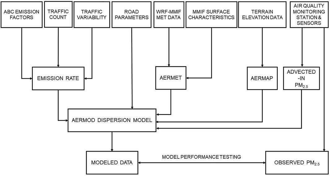
FIGURE 1. Diagram of the modeling system.
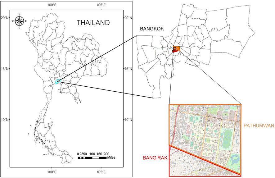
FIGURE 2. Map of the study area.
2.2 Emission inventory
An emissions inventory, classified by vehicle type, was developed at 1-h time resolution for primary PM2.5 from road vehicle exhaust for each road segment located in the study area for the period of 2018–2020. The road segments are meant for representing parts of the road with different traffic volumes. The multiyear period provides a larger set of traffic volume observations to represent traffic inhomogeneities. The emissions rate ERi for each vehicle type i for a given road section was calculated as.
where ADi represents the traffic activity data for vehicle type i and EFi represents the emissions factor for vehicle type i. Traffic activity data comprises traffic volume per time and an average traveled distance. For a given road segment, we assume the average travel distance equals the length of the road segment. The total PM2.5 emissions for a given road section is the summation of emissions rates across all vehicle types i = 1…n, where n is the total number of vehicle types. We categorized four vehicle types, namely, personal cars (PC), light-duty vehicles (LD) including vans and pick-up trucks, heavy-duty vehicles (HD) including buses and large trucks, and other vehicles (OT) including motorized three-wheelers. The details of traffic activity data, including the data sources and treatment of hourly variability, are provided in the Supplementary Material. The PM2.5 EFs categorized by vehicle type were those from the Atmospheric Brown Cloud emissions inventory manual (Shrestha et al., 2013). For PC, LD, and HD, the statistics for the case of good control-EURO I and EURO II were used. The EF used for PC was that for gasoline vehicles because 64.2% of passenger cars in Bangkok use gasoline fuel (Department of Land Transport, 2020). For other types (OT), the EF used was that for motorcycles (4-stroke with control). The EFs were 0.007, 0.15, 0.72, and 0.05 g km–1 for PC, LD, HD, and OT, respectively. The emissions rates for the four vehicle types are tabulated for each road section in the Supplementary Material.
2.3 Model setup
The American Meteorological Society (AMS)/U.S. Environmental Protection Agency (EPA) Regulatory Model (AERMOD) is a steady-state plume dispersion model that accounts for planetary boundary layer turbulence structure and is capable of handling both surface and elevated sources over both simple and complex terrain (Cimorelli et al., 2004). We used AERMOD View™ software, version 10.0.1, to conduct our simulations. The pollutant type was PM2.5. The simulation was limited to primary particulate matter.
The sources in the model were configured as line area sources because the lanes of emitting vehicles constitute a continuous line source confined in the area within the width of the road. The size of each line area source was determined by the width of the road, ranging from 10 m to 45.5 m for 2-lane to 6-lane roads, respectively. Only the main roads were designated as emissions sources. We ignored vehicle emissions from alleys and minor streets due to lack of traffic data. We assumed that these roads were far less busy than the main roads, carrying insignificant hourly average traffic volumes. The assigned emissions rates were calculated as described in the previous section. For each road segment, we set up four individual sources for the four emitting vehicle types. Each source was assigned a mean emissions rate and hourly variability factors. Ground-level Road segments were assigned their actual mean ground elevations, while expressway segments were assigned an elevation of 15 m above the actual mean ground elevation below the segment.
As for modeled processes, the model computed not only transport and dispersion but also deposition loss. The deposition calculation followed the theory described in Cimorelli et al. (2004). The particle size distribution used for emissions had a 0.99 fine particle fraction and a mean mass diameter of 0.284 microns, as calculated from the aerosol number size distribution measurement data from an urban site by Schneider et al. (2015). That site’s size distribution was selected due to its similarity to the traffic-dominated environment of the Bangkok CBD.
The discrete receptors in the model were set at 4 monitoring points, namely, Chulalongkorn Hospital, the Chulapat 14 Building, the Chulalongkorn University (CU) dormitory canteen, and Chulalongkorn Demonstration Primary School Gate 5, which we will refer to as Chula Demonstration School. In addition, grid receptors were set at a uniform spacing of approximately 130 m along each road segment over the entire modeling domain.
2.4 Input data for model
The main input data for the AERMOD simulation included meteorological data and terrain data. To account for PM2.5 originating from outside the modeling domain, we input advected-in PM2.5 concentrations. Descriptions for all data elements are provided below.
Meteorological conditions were calculated from the Weather Research and Forecasting Model (WRF) model. The meteorological data files, both for surface data and upper air data, were generated by the U.S. EPA’s Mesoscale Model Interface Program (MMIF) at the coordinate 13.73944 °N 100.5237 °E for the period of 2020. The data files were processed by the U.S. EPA’s AERMET meteorological pre-processor software, AERMET View™, version 10.2.1. The surface wind speeds and directions (blowing from) are summarized as wind rose charts in Supplementary Figure S2 in the Supplementary Material. The winds have seasonal patterns as shown for the summer (March–June), the rainy season (July–October), and the winter (November–February).
For the terrain data, we utilized the Shuttle Radar Topography Mission SRTM1 products at a resolution of 1 arc-second (30 m) with global coverage. The data were obtained via a terrain processor and downloaded through the AERMOD View program. The modeled area, in the city center, had low-lying and relatively flat terrain, with most of the area at elevations of 10–20 m and the whole area ranging from 69 m above mean sea level (MSL) to a few meters below MSL.
Since the actual PM2.5 levels in the modeling domain were influenced by both local emissions and those emitted elsewhere beyond the domain boundary, we augmented the predicted PM2.5 levels with advected-in PM2.5. Advected-in PM2.5 concentrations, which are referred to in the AERMOD View program as background concentrations, were introduced to the model by referring to the hourly PM2.5 measurements at upwind locations according to the specific wind direction at each hour. The methodology for advected-in PM2.5 is described in the Supplementary Material.
2.5 Performance evaluation
The statistical indices chosen for model testing included fractional bias (FB), correlation coefficient (R), fraction within a factor of two (FAC2), and normalized mean square error (NMSE). These indices followed the recommendations of the U.S. EPA’s “Guideline on Air Quality Models” (EPA, 2017). Past model studies have discussed the relevance and meaning of these statistical indices (Chang and Hanna, 2004; Gibson et al., 2013).
For model performance evaluation, the required PM2.5 measurement data in the study area for 2020 were downloaded from www.CUsense.net, which provides collections of PM2.5 data measured by various agencies. Measurement at the Chulalongkorn Hospital monitoring station (station ID: 50t), conducted by the Pollution Control Department, followed the official federal equivalent method (Pollution Control Department, Ministry of Natural Resource, 2010). The other three monitoring points in the Chulalongkorn University area used light-scattering sensors to measure PM2.5 (Chunitiphisan et al., 2017; 2018). Table 1 summarizes the locations of the 4 monitoring stations.
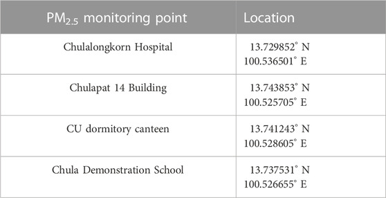
TABLE 1. The locations of the 4 monitoring stations.
3 Results and discussion
We present the simulation results for the year 2020. We attempted to conduct the simulations for 2018–2020 but determining the input data for advected-in PM2.5 for years 2018 and 2019 was challenging because of significant incidence of missing data for upwind PM2.5.
3.1 PM2.5 concentration prediction
To communicate the highest acute health risk of PM2.5 (Brook et al., 2010), the model results are presented as the maximum PM2.5 concentration found for each receptor point. Figure 3 shows the highest 24-h average PM2.5 concentration for each point in the modeling domain for the year 2020. The spatial distribution of PM2.5 in the modeling domain was very similar regardless of the time-averaging period (24-h and 1-h) or the percentile threshold. Maximum values and annual averages for the year 2020 are summarized in Table 2. The values in the domain are presented for various points among the grid receptors, including the point with the highest annual average value, a point with the mean annual average value, and the point with the lowest annual average value. The receptors of interest include the hotspot found at Phong Rama Intersection (13.746559° N, 100.520794° E) and the four monitoring points described in Table 1.
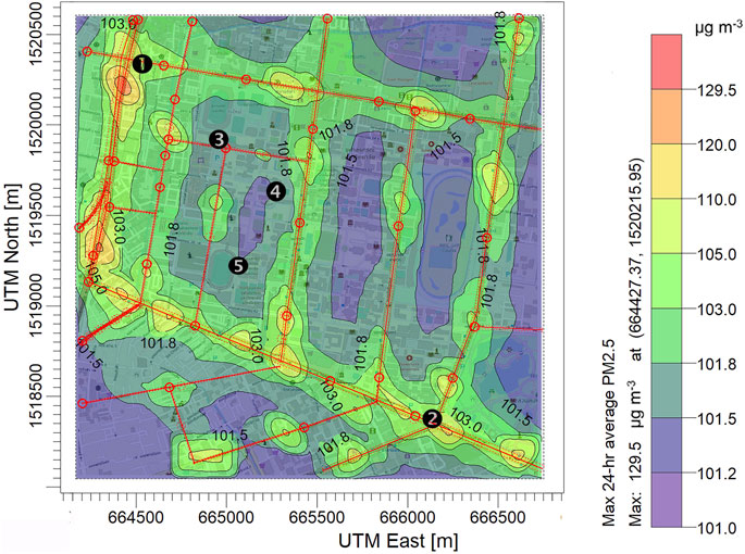
FIGURE 3. PM2.5 concentration (µg m−3) model results: Highest 24-h average for 2020. Numbered receptor points match the list in Table 2. Red lines represent emissions sources.
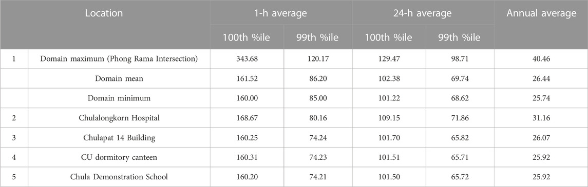
TABLE 2. Simulated high values and annual average PM2.5 concentrations (µg m−3).
The simulation revealed new information regarding the peak PM2.5 point at Phong Rama Intersection, where PM2.5 had never before been measured. The busy intersection and the expressway above this location contribute to the consistently high concentration, making it the peak PM2.5 point for all time-averaging periods. As for the remaining observation points, the Chulalongkorn Hospital observation point was located by a roadside at a busy intersection and thus exhibited higher concentrations than the other three points located in the Chulalongkorn University campus block, farther from the main public roads.
Table 2 also provides the 1-h average values in order to convey the severity of the PM2.5 situation at particular hours, while the 24-h average PM2.5 concentration is the index to be compared with the ambient standard. The value at the 99th percentile was chosen for the summary in accordance with the new World Health Organization air quality guideline for 24-h average PM2.5 concentration. The maximum 1-h average PM2.5 concentration (100th percentile value) in the domain and at each point of interest occurs in the nighttime between 00:00 and 01:00. The PM2.5 levels at the 100th percentile are significantly higher than the 99th percentile values, indicating the significant role of nighttime meteorology in creating unfavorable stagnant conditions. In the context of PM2.5 regulations, the highest PM2.5 concentration from the model agrees with the actual situation that Bangkok faces, with the 24-h average PM2.5 concentration exceeding the Thailand national ambient standards of 50 μg m−3 (as of 2020) and 37.5 μg m−3 (scheduled to begin in May 2023). As for the annual average PM2.5 concentration, comparing even the minimum point in the domain to the ambient standards of 25 μg m−3 (as of 2020) and 15 μg m−3 (enacted in July 2022), shows that the permitted standards are exceeded at all points in the domain.
Table 3 provides not only the maximum values but also the domain–average PM2.5 statistics for year 2020, including the mean, standard deviation (SD), minimum, 25th percentile, 50th percentile, 75th percentile, and maximum. The summary is calculated for the whole year as well as for each of the three seasons in order to highlight the seasonality of PM2.5 levels in Bangkok. Seasons are categorized as Summer (March–June), Rainy (July–October), and Winter (November–February). Comparing our results with those of PM2.5 models published in the literature, Peng-in et al. (2022) presented a PM2.5 model based on satellite-retrieved AOD for the Bangkok Metropolitan Region (BMR) with comparable statistics for the whole year. Their modeled domain–average PM2.5 values were lower than ours, probably because our domain lies within the CBD, which experiences intense traffic activity. In terms of seasonal statistics, our domain–average values seem to be higher and more spread than those of Peng-in et al. (2022) in the peak PM2.5 season (winter) but lower and less spread than those of Peng-in et al. (2022) in the low-PM2.5 season (rainy season). We further explore these patterns via comparisons with observations in our domain in Section 3.3.
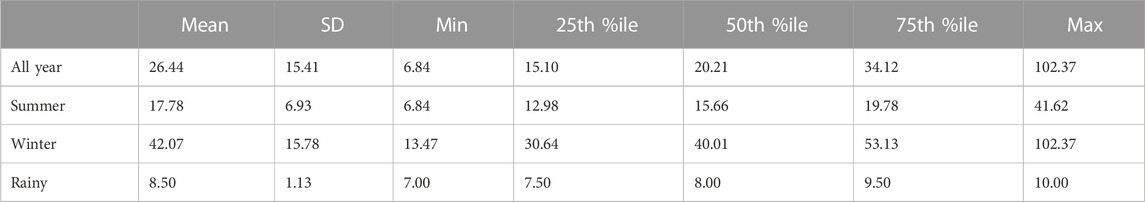
TABLE 3. 24-h average PM2.5 concentration (µg m−3): Geographic domain–average summary statistics.
3.2 Source contribution analysis
With the ability to calculate PM2.5 resulting from individual source groups as well as from all sources at once, we conducted the source contribution analysis by investigating the various road types and vehicle types. Source group is a feature in AERMOD View that lets user defines grouping of multiple sources. In the first source contribution analysis, the contributions from ground-level roads, expressways, and advection were segregated. We analyzed the source contribution information for the 2020 annual average PM2.5 for each of the 5 points of interest as shown in Figure 4A). Higher traffic volume on the expressway yielded higher emissions rates than on at-grade roads, with the expressway contributing a notably large contribution of 32.11 percent. The Chulalongkorn Hospital point showed a higher contribution from at-grade roads (17.49 percent) because of its proximity to busy at-grade roads. At the three points located in the Chulalongkorn University campus area, the main contribution came overwhelmingly from advected-in PM2.5 (∼99 percent), while the nearest main roads, situated 35–180 m away, contributed only 0.18–0.29 μg m−3 in total.
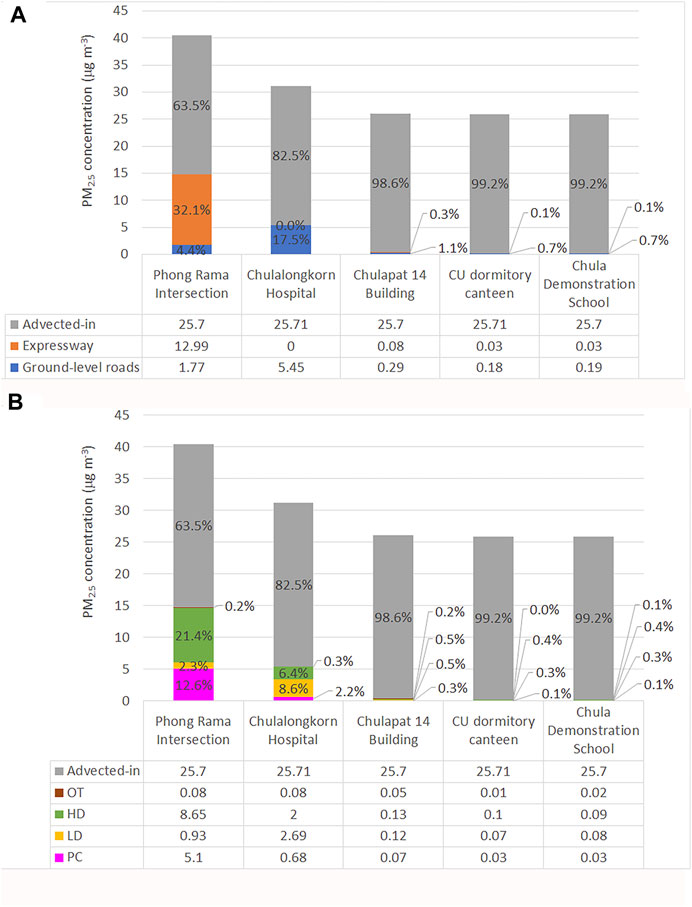
FIGURE 4. Annual average PM2.5 segregated by source contribution based on (A) road types and advection; and (B) vehicle types and advection. The concentrations are tabulated below the chart and the percentage of each source is displayed on the bar chart.
Figure 4B) provides a contribution analysis for various vehicle types as emissions sources. This analysis provides further insight to which vehicle types dominate the local PM2.5 emissions. HD showed the highest contribution at the Phong Rama Intersection because of the significant volume of heavy-duty trucks on the expressway. For the remaining points, LD showed a slightly higher contribution than HD because of the high LD traffic volume on nearby roads (averaging 18% of total traffic volume) compared to that of HD (3% on average). It is worth pointing out that the EF for HD was much higher than other vehicle types: 5 times that of LD, 14 times that of OT, and 103 times that of PC.
3.3 Model-observation comparison
Here we test the model by comparing the simulation results with PM2.5 observations as described in Section 2.5. The analysis is presented for the year 2020. Along with the statistical indices in Table 4, we present the comparison in a time-series plot, a scatter plot, and a quantile–quantile plot (Q–Q plot). We provide these visualizations for two representative receptor points, namely, Chulalongkorn Hospital and the Chulapat 14 Building as shown in Figure 5. The statistics for the 24-h average observations and predicted values are presented as a whisker box plot in Figure 6, with the data presented for the whole year of 2020 as well as separated by season. Here the median is marked by the middle line in the box, while the mean is marked by a cross sign. The bottom and the top of the box are defined by the P25* and P75* values, respectively, which are calculated from the 25th percentile (P25) and the 75th percentile (P75). Let us define P75–P25 as the interquartile range (IQR). P25* is then the larger of two values: P25 − 1.5(IQR) and the minimum value over all data. Similarly, P75* is the smaller value of two values: P75 + 1.5(IQR) and the maximum value over all data. The two ends of the whisker drawn as straight lines are the overall minimum and maximum. Solid dots represent outliers.
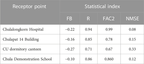
TABLE 4. Statistical indices of model–observation comparison for PM2.5 concentration.
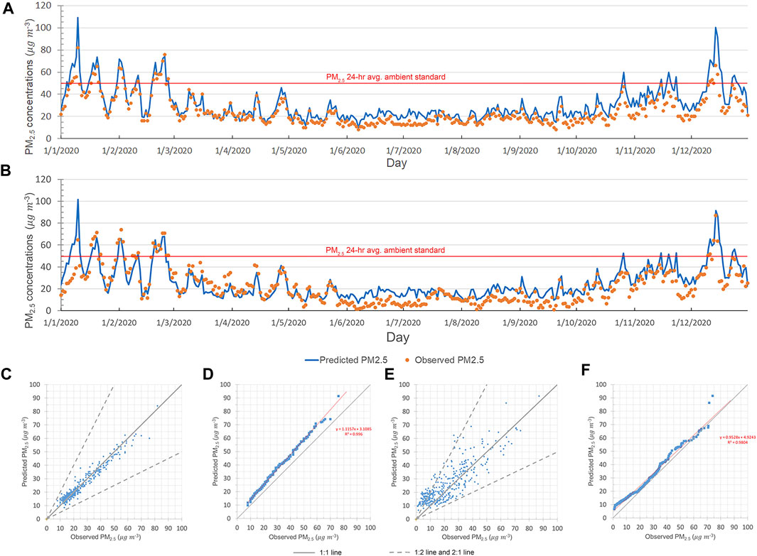
FIGURE 5. Comparisons of modeled and observed PM2.5 concentrations as (A,B) time-series plots, (C,E) scatter plots, and (D,F) Q–Q plots for (A,C,D) Chulalongkorn Hospital and (B,E,F) the Chulapat 14 Building.
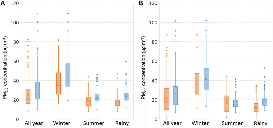
FIGURE 6. Summary of seasonal statistics for observed (orange) and modeled (blue) PM2.5 concentrations for (A) Chulalongkorn Hospital and (B) the Chulapat 14 Building.
The results for the Chulalongkorn Hospital indicate better model accuracy than those for the Chulapat 14 Building and the other two nearby sites. Temporal fluctuation in PM2.5 concentration is generally captured well in the time-series plots, with some tendency of overprediction especially in the rainy season. The whisker box plot also highlights the particularly poor modeling of the PM2.5 concentration for the rainy season, with boxes for observed and modeled data hardly overlapping. Nevertheless, the overall correlation is considered acceptable given the R values ranging from 0.71 to 0.94 for different receptor points. Model overprediction is confirmed by the FB values ranging from −0.22 to −0.10. The Q–Q plots show that the predicted PM2.5 concentrations have a distribution of values resembling that of the observed PM2.5 concentrations; thus, the data points lie along a relatively straight trendline. However, the slope of the line shows a value slightly greater than unity, reflecting the overprediction of modeled PM2.5 concentration. The acceptability of model accuracy is indicated by the scatter plots, which show data points clustering along the 1:1 line. The points lie well within the area bounded by the 2:1 line and the 1:2 line, as indicated by FAC2 values of 0.99 for Chulalongkorn Hospital and 0.78 for the Chulapat 14 Building. As presented in Table 4, the Chulalongkorn Hospital site showed the lowest NMSE value (0.08) among the points of interest, indicating the highest model accuracy. We interpret this enhanced accuracy as being due to the proximity of this site to a main road for which the emissions were well documented. The three sites in the Chulalongkorn University campus area showed poorer accuracy, especially when observed PM2.5 concentrations fell below 20 μg m−3. Because these sites were located farther from emissions sources, they received hardly any contribution from the dispersed plumes from the nearest main road sources. Therefore, at low observed PM2.5 values, PM2.5 levels were instead dominated by the advected-in contribution. We suspect that this model–observation disparity may be due in part to the model’s assumptions about advected-in PM2.5.
Another commonly reported PM2.5 pollution statistic is the number of days in each year that exceed the 24-h average ambient standard. Table 5 provides a comparison between the modeled and observed exceedance counts for the year 2020 for each of the four monitoring points as well as at the hotspot location. The modeled counts are higher than the observed counts at all sites, in line with the overprediction discussed above. The whisker box plot in Figure 6 also highlights this issue, showing several high outliers for modeled winter values in particular.
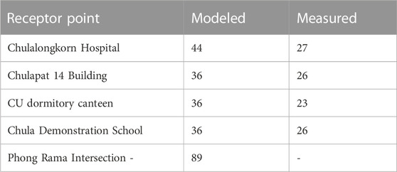
TABLE 5. 24-h average PM2.5 concentrations: Model–observation comparison of ambient standard violation count in 2020.
3.4 Discussion
In order to pave the way for future research, we now explore the model limitations encountered in utilizing the AERMOD model to produce satisfying model predictions with acceptable accuracy. Given the lack of traffic activity information with continuous time coverage, we made several assumptions based on a 1-week sample of traffic activity observed in the modeling domain as well as a monthly traffic dataset from a past study. Actual traffic may not exhibit the same hourly pattern across different roads, but modeling these differences remains an aspect for future development. Also missing from the traffic data is the additional count of motorcycles, which can be rather substantial in the domain. These known limitations of the model would be expected to result in emissions inventory underestimation. Another category of emissions that the model did not account for was non-exhaust emissions, including road surface wear, road vehicle tire wear, and brake wear (EEA, 2019). To our knowledge, there has not been a local study of the EFs of these non-exhaust emissions. We decided to ignore them because road conditions, environmental conditions, and vehicle conditions in Bangkok may differ drastically from the studied conditions in European countries, lead to high uncertainty when applying the EMEP/EEA EFs. However, these non-exhaust emissions, may potentially play a significant role. A modeling study for the city of Banská Bystrica, Slovakia, by Salva et al. (2021) showed that including non-exhaust PM2.5 emissions resulted in a total emissions rate up to 2.5 times that of exhaust emissions alone. Another limitation is the lack of chemical production calculation, causing the secondary formation of PM2.5 to go unaccounted for. However, this omission likely did not significantly affect the predicted levels. A previous source apportionment study in the BMR suggested that secondary aerosol formation may contribute ∼0.1–1 percent of ambient concentrations (Chuersuwan et al., 2008). However, recent study suggested that secondary organic carbon may contribute up to approximately 60 percent of PM2.5 (Rattanapotanan et al., 2023). Another source sector missing from the calculation is cooking which may be of importance at certain hours because there are numerous restaurants in the study area. There has never been a study to account for such emission rates to our knowledge.
Regarding the source contribution analysis, we found the dominant influence in the model was advected-in PM2.5. Our assumption of a two-box model (described in the Supplementary Material) and referencing of upwind roadside monitoring data might have introduced an excessive PM2.5 level that led to an overall overestimation by the model despite the several factors discussed above that contribute toward underestimation. The burden of adding advected-in PM2.5 to achieve good agreement with observed PM2.5 levels is a trade-off for using a dispersion model such as AERMOD, which is relatively easier to implement than a regional chemical transport model. Future work may explore the ways in which including non-exhaust emissions might lower the influence of advected-in PM2.5 on the model.
To investigate the contributions of local sources, we compare our findings with those of a previous study in a similar setting. In our comparison with Salva et al. (2021)’s AERMOD simulations in a city in Slovakia, we focus on the relative contributions of exhaust emissions from various vehicle types. Salva et al. (2021) assigned the EFs based on fuel type (petrol vs. diesel) and technology (EURO2 to EURO6), while we chose a simpler treatment with a single EF value for each vehicle type due to lack of actual vehicle fleet data. Comparing the emissions factors that we used with those in Salva et al. (2021) for the same vehicle types for the technology (EURO-X) with the highest population, we found that our EFs were higher for all vehicle types. Our EF for HD was 103 times that for PC, while our AADTPC:AADTHD, traffic volume ratio lay in the range of 9–117 with a mean value of 35. Accordingly, the model shows HD emissions surpassing PC emissions for almost all represented road segments in the domain. Salva et al. (2021) found that among the exhaust emissions sources for the study domain, PC provided the largest contribution, while we found that HD and LD provided the largest contributions for the receptor points dominated by expressway and ground-level urban roads, respectively. This difference between study domains is in line with the technological reality of trucks in Thailand: mostly EURO2 or at best EURO4.
Our PM2.5 model for the Bangkok CBD can provide new insights into PM2.5 models including previously developed models that used different techniques and tools (Ketjumpol and Sakworawich, 2020; Chalermpong et al., 2021; Kumharn et al., 2022; Peng-In et al., 2022; Thongthammachart et al., 2023). The variability in emissions rates from time-varying traffic data may provide an in-depth tool to investigate the particular incidence of extreme health risks posed by PM2.5. Such analysis can support the decision to tackle precise sources driving PM2.5 peaks.
Given the points discussed above, potential research that builds upon these lessons may utilize comprehensive continuous traffic surveillance with the aid of artificial intelligence. Such research may further develop this concept of emissions inventory calculation into a regional chemistry transport model to provide a complete representation of PM2.5 sources in a wider region not limited to a small geographic domain of interest. Another opportunity to enhance the knowledge of PM2.5 for Bangkok air quality management would be the inclusion of PM2.5 sources other than road traffic. We note that these potential research directions emphasize the need for an updated, accurate emissions inventory at high spatiotemporal resolution for effective local air quality management.
3.5 Scenario study
We demonstrate the utility of the model as a decision-making support tool by studying PM2.5 mitigation scenarios from the National Agenda Action Plan to Eradicate Particulate Matter Pollution Problem (Pollution Control Department, 2019). Two PM2.5 mitigation scenarios from the action plan were chosen, namely, the fuel standard (FS) scenario and the shift mode (SM) scenario. The simulation period is the year 2020. The effects of each mitigation measure are reflected in the emissions rate calculation as described below. Advected-in PM2.5 concentrations were kept the same as in the base case simulation as described in Section 2 because the result of each policy cannot be effectively estimated in a regional context. With this limitation, we do not anticipate realistic modeled PM2.5 levels in the studied scenarios. However, even unrealistic model results can provide valuable comparative information in determining which policy results in a better improvement with regard to PM2.5 levels.
The FS scenario refers to the measure to upgrade emissions standards to EURO6 by the year 2022; however, we note that in reality this upgrade has not been achieved as of January 2023 and also the new EURO6 standard is enforced on new vehicles only. This change was modeled by altering the emissions factors for the four types of vehicles as shown in Table 6. The EURO6 EFs are taken from Kim Oanh (2020). The resulting change in emissions rates on each road segment then depends on the traffic volume classification by vehicle type. In this scenario, we assumed 100 percent replacement of the existing fleets running in the modeling domain by new vehicles meeting the EURO6 emissions standards. The changes in PM2.5 level (not shown) occur almost entirely as decreases with respect to the base case. The reduction is pronounced along the main road and especially along the expressway alignment because of the high total emissions in the area. The one slight increase in PM2.5 occurs on a road segment where the traffic data shows a particularly high portion of motorized three-wheelers. The rather counterintuitive EF increase for three-wheelers under the EURO6 standard, categorized as OT, results in this small increase.
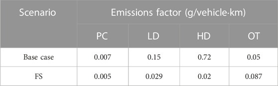
TABLE 6. Emissions factors for the four vehicle types.
The SM scenario refers to a measure that promotes public transportation and lower-emissions modes such as bicycling. The assumption in this scenario is that PC traffic volume is lowered by 70 percent while other vehicle traffic volume is reduced by 50 percent compared to the traffic volume in the base case. The shift away from PC, including taxi usage, as well as away from three-wheeled taxi usage, would translate to higher passenger counts on mass transit electrified rail systems and, possibly, electric buses, thus result in no additional local PM2.5 exhaust emissions. The reduced traffic volume data fed into the emissions inventory calculation results in lower overall emissions. The PM2.5 reduction is found to be most significant along the expressway alignment, just as in the FS scenario, again because of the high PC volume on the expressway.
To compare the results of the two PM2.5 mitigation scenarios, we consider the count of days in each year that exceed the 24-h average ambient standard 50 μg m−3 at the points of interest under each scenario and in the base case. As shown in Table 7, the FS scenario proved more effective at lowering PM2.5 levels below the 50 μg m−3 threshold. The results at the three receptor points in the Chulalongkorn University campus area were not affected in either scenario because their dominant contribution was from advected-in PM2.5; the results are therefore not shown.
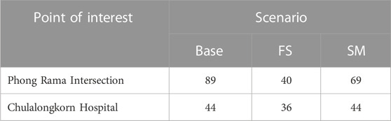
TABLE 7. 24-h average PM2.5 concentrations: Ambient standard violation counts in various scenarios.
4 Conclusion
This work presented a proof of concept in utilizing traffic observation data classified by vehicle type for the calculation of a PM2.5 emissions inventory for road traffic sources in the study domain, here the Bangkok CBD. The model results revealed a PM2.5 hotspot location at Phong Rama Intersection near the expressway, where PM2.5 has never before been monitored. The peak 1-h average PM2.5 concentration was 343.68 μg m−3, while the peak 24-h average PM2.5 concentration was 129.47 μg m−3.
This analysis presented new information for the planning of air quality and health monitoring. The source contribution analysis of annual average PM2.5 indicated a contribution from expressway traffic being 32 percent for the location near the expressway, while an at-grade roadside receptor farther from the expressway might receive a contribution of 17.5 percent from ground-level roads but none from the expressway. In each case, the substantial remaining portion was attributable to advection from outside the modeling domain. For receptor points inside the University campus, almost all PM2.5 was due to advection from outside the modeling domain. Another view of the source contribution analysis for vehicle types revealed HD and LD as the top contributors of locally emitted PM2.5. Advected-in PM2.5 was the most dominant fraction overall, highlighting the transboundary nature of air pollution and the need for solutions that extend beyond a given small area. The model testing results showed acceptable agreement between modeled and observed 24-h average PM2.5 levels, with the model tending to overpredict. The model was utilized in a scenario study to demonstrate its usefulness as a tool to support decision-making in the selection of PM2.5 abatement measures. We compared the PM2.5 mitigation effectiveness of two measures from the National Agenda Action Plan to Eradicate Particulate Matter Pollution, namely the FS upgrade and the promotion of a travel mode shift. We found that the FS upgrade measure resulted in a greater reduction in the number of days in each year that exceed the 24-h average ambient standard.
Data availability statement
The original contributions presented in the study are included in the article/Supplementary Material, further inquiries can be directed to the corresponding author.
Author contributions
TR and WT contributed to the study conception and design. WT contributed the calculation method for the emission inventory and TR carried out data collection and calculation. Model simulations were performed and analyzed by TR with post-processing programming supported by WT. The first draft of the manuscript was written by TR and subsequent edits were done by WT. All authors contributed to the article and approved the submitted version.
Funding
This work was conducted as part of the Impactful and Innovation Research Platform: Sustainable Environment supported by the Ratchadaphisek Sompoch Endowment Fund (2022), Chulalongkorn University, under the Grant Contract No. 765007-RES02. Traffic emissions data development in its early stage was conducted under the Air Quality Measurement and Functional Areas of Selected Urban Park project of the Center of Excellence on Hazardous Substance Management.
Acknowledgments
We appreciate the support of Miss Katathikan Laungdumrongsak, who at the time of her involvement was a student of the Department of Environmental Engineering, Chulalongkorn University, in the preparation of data input for the emission calculation. We acknowledge Thailand Network Center on Air Quality Management (TAQM) and EnvGIT for their support of CUSense monitoring data.
Conflict of interest
The authors declare that the research was conducted in the absence of any commercial or financial relationships that could be construed as a potential conflict of interest.
Publisher’s note
All claims expressed in this article are solely those of the authors and do not necessarily represent those of their affiliated organizations, or those of the publisher, the editors and the reviewers. Any product that may be evaluated in this article, or claim that may be made by its manufacturer, is not guaranteed or endorsed by the publisher.
Supplementary material
The Supplementary Material for this article can be found online at: https://www.frontiersin.org/articles/10.3389/fenvs.2023.1237366/full#supplementary-material
References
Afzali, A., Rashid, M., Afzali, M., and Younesi, V. (2017). Prediction of air pollutants concentrations from multiple sources using AERMOD coupled with WRF prognostic model. J. Clean. Prod. 166, 1216–1225. doi:10.1016/j.jclepro.2017.07.196
Askariyeh, M. H., Kota, S. H., Vallamsundar, S., Zietsman, J., and Ying, Q. (2017). AERMOD for near-road pollutant dispersion: Evaluation of model performance with different emission source representations and low wind options. Transp. Res. Part D Transp. Environ. 57, 392–402. doi:10.1016/j.trd.2017.10.008
Brook, R. D., Rajagopalan, S., Pope, C. A., Brook, J. R., Bhatnagar, A., Diez-Roux, A. V., et al. (2010). Particulate matter air pollution and cardiovascular disease: An update to the scientific statement from the American Heart Association. Circulation 121 (21), 2331–2378. doi:10.1161/CIR.0b013e3181dbece1
Chalermpong, S., Thaithatkul, P., Anuchitchanchai, O., and Sanghatawatana, P. (2021). Land use regression modeling for fine particulate matters in Bangkok, Thailand, using time-variant predictors: Effects of seasonal factors, open biomass burning, and traffic-related factors. Atmos. Environ. 246, 118128. doi:10.1016/j.atmosenv.2020.118128
Chang, J. C., and Hanna, S. R. (2004). Air quality model performance evaluation. Meteorology Atmos. Phys. 87 (1-3). doi:10.1007/s00703-003-0070-7
Chavanaves, S., Fantke, P., Limpaseni, W., Attavanich, W., Panyametheekul, S., Gheewala, S. H., et al. (2021). Health impacts and costs of fine particulate matter formation from road transport in Bangkok Metropolitan Region. Atmos. Pollut. Res. 12 (10), 101191. doi:10.1016/j.apr.2021.101191
Chuersuwan, N., Nimrat, S., Lekphet, S., and Kerdkumrai, T. (2008). Levels and major sources of PM2.5 and PM10 in Bangkok metropolitan region. Environ. Int. 34 (5), 671–677. doi:10.1016/j.envint.2007.12.018
Chunitiphisan, S., Panyamethekul, S., Pumrin, S., Tanaksaranond, G., and Ngamsritrakul, T. (2018). Particulate matter monitoring using inexpensive sensors and internet gis: A case study in nan, Thailand. Eng. J. 22 (2), 25–37. doi:10.4186/ej.2018.22.2.25
Chunitiphisan, S., Panyamethekul, S., and Tanaksaranond, G. (2017). Development of a sensor network and geospatial system to monitor and monitor the haze situation in Northern Thailand. Thailand Research Fund.
Cimorelli, A., Perry, S., Venkatram, A., Weil, J., Paine, R., Wilson, R., et al. (2004). Aermod: Description of model formulation, US environmental protection agency. EPA-454/R-03-004.
Department of Land Transport (2020). Number of registered vehicles (cumulative) classified by type of fuel as of December 31, 2020. Available online at: https://web.dlt.go.th/statistics/ (Accessed October 15, 2022).
Environmental Protection Agency (EPA) (2017). Revisions to the guideline on air quality models: Enhancements to the AERMOD dispersion modeling system and incorporation of approaches to address ozone and fine particulate matter. Available online at: https://www.epa.gov/sites/default/files/2020-09/documents/appw_17.pdf (Accessed November 24, 2022).
European Environment Agency (EEA) (2019). EMEP/EEA air pollutant emission inventory guidebook 2019. Available online at: https://www.eea.europa.eu/publications/emep-eea-guidebook-2019 (Accessed November 17, 2022).
Gibson, M. D., Kundu, S., and Satish, M. (2013). Dispersion model evaluation of PM2.5, NOx and SO2 from point and major line sources in Nova Scotia, Canada using AERMOD Gaussian plume air dispersion model. Atmos. Pollut. Res. 4 (2), 157–167. doi:10.5094/apr.2013.016
Gulia, S., Shiva Nagendra, S. M., and Khare, M. (2014). Performance evaluation of ISCST3, adms-urban and aermod for urban air quality management in a mega city of India. Int. J. Sustain. Dev. Plan. 9 (6), 778–793. doi:10.2495/sdp-v9-n6-778-793
Hanma, P. (2021). Extent and magnitude of industrial stack emissions on ambient particulate concentrations. Int. J. GEOMATE 21 (84). doi:10.21660/2021.84.j2189
IQAir (2021). World air quality report region & city PM2.5 ranking. Available online at: https://www.iqair.com/th-en/world-most-polluted-countries (Accessed October 12, 2022).
Katika, K., and Karuchit, S. (2018). “Estimation of urban air pollutant levels using AERMOD: A case study in nakhon ratchasima, Thailand,” in IOP conference series: Earth and environmental science (Kuala Lumpur, Malaysia: IOP Publishing), 012024.
Ketjumpol, T., and Sakworawich, A. (2020). Time series models predicting fine particulate matter in Bangkok. J. Appl. Statistics Inf. Technol. 4 (2), 46–63.
Kim Oanh, N. T. (2020). Final report on the study of sources of particulate matter less than 2.5 microns (PM2.5) and secondary pollutants (Secondary PM2.5) in Bangkok and surrounding areas. Thailand.
Kumharn, W., Sudhibrabha, S., Hanprasert, K., Janjai, S., Masiri, I., Buntoung, S., et al. (2022). Improved hourly and long-term PM2.5 prediction modeling based on MODIS in Bangkok. Remote Sens. Appl. Soc. Environ. 28, 100864. doi:10.1016/j.rsase.2022.100864
Office of Natural Resources and Environmental Policy and Planning (ONEP). (2021). Report on the situation of environmental quality in 2020. Thailand.Office of natural resources and environmental policy and planning
Peng-In, B., Sanitluea, P., Monjatturat, P., Boonkerd, P., and Phosri, A. (2022). Estimating ground-level PM(2.5) over Bangkok Metropolitan Region in Thailand using aerosol optical depth retrieved by MODIS. Air Qual. Atmos. Health 15 (11), 2091–2102. doi:10.1007/s11869-022-01238-4
Pollution Control Department (2019). The national Agenda action plan to eradicate PM2.5 issue. Thailand.
Pollution Control Department, Ministry of Natural Resources and Environment (2010). Notification of the pollution control department: Method for measuring the average value of particulate matter size less than 2.5 microns. Thailand.
Rattanapotanan, T., Thongyen, T., Bualert, S., Choomanee, P., Suwattiga, P., Rungrattanaubon, T., et al. (2023). Secondary sources of PM2.5 based on the vertical distribution of organic carbon, elemental carbon, and water-soluble ions in Bangkok. Environ. Adv. 11, 100337. doi:10.1016/j.envadv.2022.100337
Salva, J., Vanek, M., Schwarz, M., Gajtanska, M., Tonhauzer, P., and Ďuricová, A. (2021). An assessment of the on-road mobile sources contribution to particulate matter air pollution by AERMOD dispersion model. Sustainability 13 (22), 12748. doi:10.3390/su132212748
Schneider, I. L., Teixeira, E. C., Silva Oliveira, L. F., and Wiegand, F. (2015). Atmospheric particle number concentration and size distribution in a traffic–impacted area. Atmos. Pollut. Res. 6 (5), 877–885. doi:10.5094/apr.2015.097
Seangkiatiyuth, K., Surapipith, V., Tantrakarnapa, K., and Lothongkum, A. W. (2011). Application of the AERMOD modeling system for environmental impact assessment of NO2 emissions from a cement complex. J. Environ. Sci. 23 (6), 931–940. doi:10.1016/s1001-0742(10)60499-8
Shrestha, R., Kim Oanh, N., Shrestha, R., Rupakheti, M., Permadi, D., Kanabkaew, T., et al. (2013). Atmospheric Brown Cloud (ABC) emission inventory manual (EIM). Nairobi, Kenya: United Nation Environmental Programme.
Thongthammachart, T., Shimadera, H., Araki, S., Matsuo, T., and Kondo, A. (2023). Land use regression model established using Light Gradient Boosting Machine incorporating the WRF/CMAQ model for highly accurate spatiotemporal PM2.5 estimation in the central region of Thailand. Atmos. Environ. 297, 119595. doi:10.1016/j.atmosenv.2023.119595
Tran, Q. B., Lohitnavy, M., and Phenrat, T. (2019). Assessing potential hydrogen cyanide exposure from cyanide-contaminated mine tailing management practices in Thailand's gold mining. J. Environ. Manage 249, 109357. doi:10.1016/j.jenvman.2019.109357
Keywords: fine particulate pollution, PM2.5, air dispersion model, source contribution analysis, traffic emission inventory, AERMOD
Citation: Ratanavalachai T and Trivitayanurak W (2023) Application of a PM2.5 dispersion model in the Bangkok central business district for air quality management. Front. Environ. Sci. 11:1237366. doi: 10.3389/fenvs.2023.1237366
Received: 09 June 2023; Accepted: 10 July 2023;
Published: 20 July 2023.
Edited by:
Thongchai Kanabkaew, Thammasat University, ThailandReviewed by:
Sudjit Karuchit, Suranaree University of Technology, ThailandÖzgür Zeydan, Bülent Ecevit University, Türkiye
Copyright © 2023 Ratanavalachai and Trivitayanurak. This is an open-access article distributed under the terms of the Creative Commons Attribution License (CC BY). The use, distribution or reproduction in other forums is permitted, provided the original author(s) and the copyright owner(s) are credited and that the original publication in this journal is cited, in accordance with accepted academic practice. No use, distribution or reproduction is permitted which does not comply with these terms.
*Correspondence: Win Trivitayanurak, d2luLnRAY2h1bGEuYWMudGg=