 Manzhu Yu
 Shiyan Zhang1
 Kai Zhang
 Matthew Varela
 Jiheng Miao
94% of researchers rate our articles as excellent or good
Learn more about the work of our research integrity team to safeguard the quality of each article we publish.
Find out more
ORIGINAL RESEARCH article
Front. Environ. Sci., 13 July 2023
Sec. Big Data, AI, and the Environment
Volume 11 - 2023 | https://doi.org/10.3389/fenvs.2023.1223160
Introduction: Traditional methods to estimate exposure to PM2.5 (particulate matter with less than 2.5 µm in diameter) have typically relied on limited regulatory monitors and do not consider human mobility and travel. However, the limited spatial coverage of regulatory monitors and the lack of consideration of mobility limit the ability to capture actual air pollution exposure.
Methods: This study aims to improve traditional exposure assessment methods for PM2.5 by incorporating the measurements from a low-cost sensor network (PurpleAir) and regulatory monitors, an automated machine learning modeling framework, and big human mobility data. We develop a monthly-aggregated hourly land use regression (LUR) model based on automated machine learning (AutoML) and assess the model performance across eight metropolitan areas within the US.
Results: Our results show that integrating low-cost sensor with regulatory monitor measurements generally improves the AutoML-LUR model accuracy and produces higher spatial variation in PM2.5 concentration maps compared to using regulatory monitor measurements alone. Feature importance analysis shows factors highly correlated with PM2.5 concentrations, including satellite aerosol optical depth, meteorological variables, vegetation, and land use. In addition, we incorporate human mobility data on exposure estimates regarding where people visit to identify spatiotemporal hotspots of places with higher risks of exposure, emphasizing the need to consider both visitor numbers and PM2.5 concentrations when developing exposure reduction strategies.
Discussion: This research provides important insights for further public health studies on air pollution by comprehensively assessing the performance of AutoML-LUR models and incorporating human mobility into considering human exposure to air pollution.
Exposure to air pollution can directly affect human health and increase healthcare use (Reid et al., 2016; Black et al., 2017). The World Health Organization (WHO) estimates that 4.2 million deaths annually can be attributed to outdoor air pollution (Shaddick et al., 2020). Among various types of air pollutants, fine particle (PM2.5) is an air pollutant that is a concern for people’s health as it penetrates the lungs and circulatory system, contributing ∼98% to ∼7 million deaths globally (Butt et al., 2017; WHO, 2022). PM2.5 often comes from various emission sources, including the combustion of gas, oil, diesel fuel, and wood, industrial processes, power generators, and natural phenomena, such as wildfires, dust storms, and volcanic eruptions (McDuffie et al., 2021). The accurate and frequent monitoring of PM2.5 is crucial to notify citizens of potentially poor air quality, as the concentration of PM2.5 at a particular location might change rapidly depending on the emission sources, wind speed, wind direction, and other meteorological factors (Sun et al., 2022). Regulatory monitors from local and U.S. Environmental Protection Agencies (EPA) have played an indispensable role in measuring local air quality but are limited in their sparse distribution and high cost of maintenance and deployment.
The development of low-cost air quality sensors, such as PurpleAir and Clarity sensors, provides new opportunities for capturing air quality dynamics in a high spatial and temporal resolution (Gupta et al., 2018; Caubel et al., 2019; Fowlie et al., 2020). These sensors are not only cost-effective and easy to deploy but can also wirelessly transmit the data they gather, providing a contrast to the traditional, complex, and expensive regulatory air monitoring stations. PurpleAir sensors use dual laser particle counters that can provide a more detailed view of particulate pollution. Clarity sensors work by measuring the attenuation of infrared radiation in the air. They consist of an infrared radiation source, a light-water tube, and an infrared detector with an appropriate filter. New insights have been discovered using the low-cost sensor networks regarding the spatial patterns of air quality on a local or neighborhood scale (Weissert et al., 2020; Kelly et al., 2021), local influences of emission sources (Zimmerman et al., 2020; Lu et al., 2021), and fine-scaled human exposure assessments (Bi et al., 2022). Calibrations and correction methods have been developed to improve the data plausibility compared to regulatory monitors (Tryner et al., 2020; Barkjohn et al., 2021; Wallace et al., 2021).
Land use regression (LUR) models are commonly used in air pollution exposure assessment to produce averaged exposure risks in a temporal range with a high spatial resolution (Beelen et al., 2014; Li et al., 2020; Ren et al., 2020). LUR models are particularly useful for identifying spatial features that are important determinants of pollutant concentration variability and for enhancing our understanding of the spatial distribution of air pollutants (Meng et al., 2015; Lee et al., 2017; Muttoo et al., 2018). These models are based on the assumption that the average air quality within a specific area is linearly associated with geographic covariates such as land use, road density, and emission sources (Hoek et al., 2008). The LUR modeling process generally involves the preparation of such covariates, creating LUR models by linear regression while selecting variables that are highly correlated with the model and avoiding redundant variables, validating and selecting the final model, and applying the final model to a high-resolution grid for the area where predictions are to be made (Morley and Gulliver, 2018; Ma et al., 2020). The integration of low-cost sensors and regulatory monitors in LUR models also showed the potential of better capturing within-city variations (Lu et al., 2022). However, LUR models generally suffer from their limitations in area generalizability: a LUR model developed for a particular area within a specific time range cannot be easily adopted, and models have to be re-developed for any other spatiotemporal range (Bi et al., 2022). In addition, while timely-averaged (e.g., annual or multi-year) concentrations could reduce the biases resulting from a few high-level outliers, it is essential to develop PM2.5 exposure models at finer temporal resolutions (e.g., daily or hourly) for a more frequent assessment of air pollution exposure (Masiol et al., 2018; Lu et al., 2021).
Recent studies have improved LUR models to address the limitations using generalized additive models (Ravindra et al., 2019), principal component analysis (de Souza et al., 2018), Least Absolute Shrinkage and Selection Operator (LASSO) (Roberts and Martin, 2005), and Bayesian inference (Thomas et al., 2007; Orun et al., 2018; Han et al., 2022). Spatial and temporal variations captured at a high spatial and temporal resolution can reveal conditions where air quality differs from the expected land-use effect (Weissert et al., 2020). Machine learning approaches, especially ensemble-based methods such as random forests, have provided a non-parametric solution without assuming a linear relationship between air pollutant concentration and the predictors (Ren et al., 2020; Coker et al., 2021; Jain et al., 2021; Wong et al., 2021); instead, complex relationships can be captured within such models. Specifically, Weissert et al. (2020) applied a random forest model to data from a low-cost sensor network to analyze the impact of land use on local air quality and to capture air quality variations on an hourly basis at a detailed spatial scale. Coker et al. (2021) explored various ML base-learner and ensemble algorithms to improve LUR predictions in monthly PM2.5 in urban regions of central and eastern Uganda. Kelly et al. (2021) developed a Gaussian process model to accurately predict neighborhood-scale PM2.5 concentrations during pollution events such as fireworks, wildfires, and persistent cold air pools.
In addition, integrating time-varying predictors (e.g., meteorological conditions and satellite-retrieved aerosol optical depth) has also improved LUR models’ temporal resolution to daily or hourly (Masiol et al., 2018; Yao et al., 2018; Lu et al., 2021). Combining the predictor selection procedure in LUR and the ML-based prediction model in estimating the non-linear relationships has been explored to leverage both advantages into an integrated framework (Jain et al., 2021; Wong et al., 2021). A particular challenge in hourly LUR modeling is the availability of satellite-observed aerosol optical depth (AOD). Most existing studies rely on MODIS AOD product, which has an overpass of twice daily and in the afternoon. The limited availability of satellite-observed AOD hampers the ability of LUR models to predict hours that are outside these overpassed times. This is also one of the reasons why LUR models are used mostly for monthly or yearly assessments of air pollution.
Human exposure to air pollution has been a longstanding concern in public policy. Epidemiologic evidence demonstrated causal relationships between particulate matter (PM) and health outcomes and revealed disparities between different groups regarding their risks of related health effects (Jbaily et al., 2022). Exposure risks are generally calculated based on pollutant concentrations and the population affected by the pollutants. Environmental agencies have been providing online dashboards for public showcases of environmental justice (EJ) related to air pollution, e.g., the U.S. EPA’s EJScreen and CalEnviroScreen. These approaches fail to account for all components of exposure since 1) there might be a high spatial and temporal variability of air pollutant concentrations, and 2) people spend time both in places they live and visit (Canha et al., 2021). Human exposure studies have considered physical movements and activities of individuals and the environments in which they spend their time. Most of these studies rely on individual mobility patterns inferred from mobile phone data or Call Detail Record (CDR) data collected by mobile network operators (Nyhan et al., 2016; 2019; Yu et al., 2020), but focused on a particular area and in a limited time window. Comprehensive studies across different spatial regions are necessary to accurately assess the risks of air pollution and inform public health policy. These studies can help to identify patterns of exposure and potential health risks and can inform the development of strategies to reduce or eliminate exposure to harmful substances.
This research proposes an empirical foundation by integrating machine learning and low-cost sensor measurements into estimating spatiotemporal variability of PM2.5 concentrations in eight major metropolitan areas in the U.S. and assessing exposure to PM2.5 based on where people visit. We integrate the measurements of PM2.5 from a low-cost sensor network (PurpleAir) with EPA’s regulatory monitors into LUR model development. We use a LUR model based on automated machine learning, i.e., AutoML-LUR, to capture the relationship between geographic covariates and PM2.5 concentrations. In addition, we take human mobility into consideration of human exposure regarding where people visit and investigate how mobility impact exposure estimates. Details on the methods used in this study are presented in the next section, followed by the results of the study and a discussion of the potential of the methods and data, as well as associated limitations.
Our analyses aimed to assess data and modeling performance from multi-city low-cost sensors and existing regulatory monitoring networks. We selected core-based statistical areas (CBSAs) with at least seven EPA regulatory monitors and seven PurpleAir sensors between 1 January 2018, and 31 December 2021 (Table 1). The choice of requiring at least seven sensors from each type (EPA monitors and PurpleAir sensors) in the study is based on our goal to ensure a sufficient spatial coverage for LUR models. The specific number, seven, is chosen in reference to Lu et al. (2022), which deployed seven sensors of each type in six cities across the United States, and this configuration showed promising results in assessing data and modeling performance for low-cost sensors in different urban environments. Following this approach, we aimed to ensure a similar level of representativeness in our analyses.
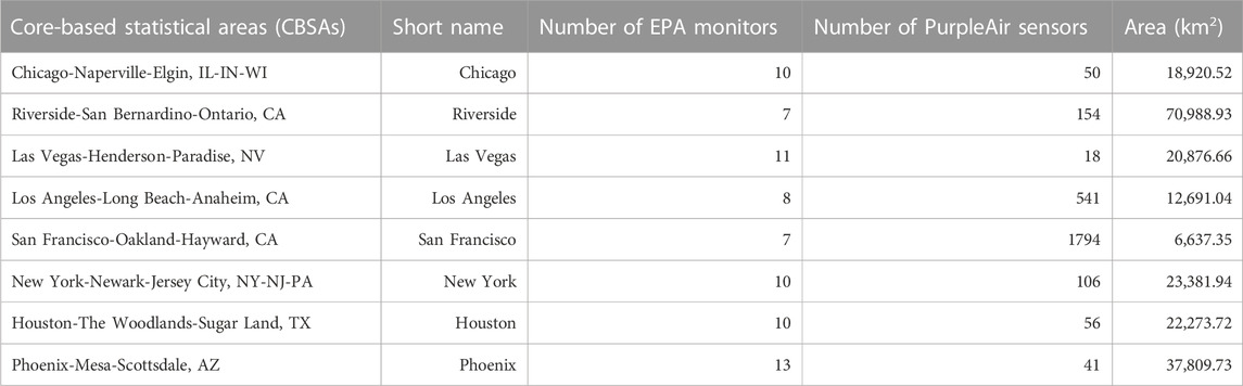
TABLE 1. Selected core-based statistical areas in the study, 2018–2021.
Hourly PM2.5 measurements are downloaded from the EPA Air Quality System (AQS) database for Federal Reference Method (FRM) monitors and Federal Equivalent Method (FEM) monitors. In addition, we downloaded publicly available outdoor PM2.5 measurements from the PurpleAir website via an open-source R package: AirSensor, developed by the South Coast Air Quality Management District (South Coast AQMD) and Mazama Science. The raw data was aggregated into hourly averages using the quality control function provided by AirSensor. The function creates a PM2.5 time series by averaging the A and B channels and removing the invalidate date when 1) the measurement count is lower than 20, 2) the hourly difference between A and B channels is higher than 5, and 3) the hourly percent difference between A and B channels is higher than 70%. Samples with PM2.5 measurements greater than 1,000 μg/m3 and with missing or abnormal temperature and humidity readings were removed (humidity readings should be within 0%–100%; temperature readings should be within 20°F to 140°F). Approximately 15% of the raw PurpleAir measurements were removed due to these quality issues. We applied the correction to the PurpleAir PM2.5 measurements based on the U.S.-wide calibration proposed by Barkjohn et al. (2021).
Comparing the monthly hourly PM2.5 concentrations between EPA and PurpleAir in the selected study regions (Figure 1), measurements from the PurpleAir sensors generally have a lower median value than the EPA monitors. There could be several reasons why EPA air quality measurements are consistently higher than PurpleAir measurements. One reason could be that the EPA uses more sophisticated and expensive air quality monitoring equipment, which is subject to strict quality control and calibration procedures to ensure the accuracy of the measurements. In contrast, PurpleAir monitors are designed for personal use and are not subject to the same level of quality control and calibration, which can lead to a more significant margin of error in the readings. Another reason could be the placement of the monitors. The EPA often selects monitoring sites based on strict criteria to ensure that they represent the air quality in a given area (Raffuse et al., 2007). In contrast, PurpleAir monitors are typically installed by individuals in their own homes or businesses, and the placement of the monitors can vary widely (Ardon-Dryer et al., 2020). It is also worth noting that the EPA and PurpleAir use different methods to measure air quality. The EPA primarily measures PM2.5 using gravimetric analysis, while PurpleAir uses a laser-based sensor technology. While both methods are considered reliable, they can produce slightly different measurements depending on factors such as humidity and temperature.
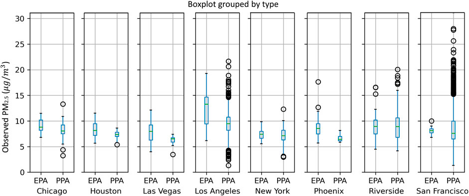
FIGURE 1. Boxplots of PM2.5 concentrations measured by EPA monitors and PurpleAir monitors in eight metropolitan areas. Each box extends from the first quartile (Q1) to the third quartile (Q3) of the data, with a line at the median. The whiskers extend from the box by 1.5x the interquartile range (IQR). Outlier points are those past the end of the whiskers.
Traditional LUR models are statistical methods developed to estimate PM2.5 concentrations based on geographical features. The models can create an empirical relationship between PM2.5 concentrations and land use variables such as traffic volume, distance to major roads, population density, and presence of emission sources. A typical LUR model can be formulated as:
where
In this study, we used automated machine learning (detailed in Section 2.3.3) to construct more sophisticated versions of LUR models. Traditional LUR models, illustrated in Eq. 1, use multiple linear regression, which assumes a linear relationship between predictor variables and the target outcome. However, real-world relationships between land-use variables and PM2.5 concentrations may be nonlinear or involve complex interactions, which can be better captured with machine learning techniques.
We analyzed 4 years of available PM2.5 concentration data for LUR modeling. Hourly measurements of PM2.5 concentration were used to compute monthly averages for each hour (e.g., January 2021 will have 24 h averages; monthly-hourly thereafter). These monthly-hourly averages were used to train and test the LUR models. To test the usefulness of low-cost sensor networks for developing AutoML-LUR models, we developed three types of models 1) using the EPA measurements, 2) using the PurpleAir measurements, and 3) incorporating PM2.5 measurements from EPA monitors and PurpleAir sensors for the eight CBSAs. For each monitoring location, we prepare the geographic covariates following the guidelines from the Multi-Ethnic Study of Atherosclerosis and Air Pollution (Keller et al., 2015; Kirwa et al., 2021).
The initial set of geographic covariates for LUR modeling contains proximity and buffer variables regarding land-use categories, emission sources, and vegetation indices (Keller et al., 2015; Kirwa et al., 2021). Proximity variables include distances to major land use categories, roads and truck routes, airports, coastlines and railroads, ports, and point emission sources. Buffer variables include summarized statistics of spatial features within a group of buffer ratios (0.5–30 km). These features include the sum of road or truck route length, total emission, percentiles of NDVI, average imperviousness value, and average elevation, respectively, calculated in buffers. Beyond the time-invariant variables suggested in MESA Air, we also added time-varying variables that account for the complex dynamics of air pollutant concentrations, such as meteorological conditions and satellite-retrieved aerosol optical depth (AOD). The complete list of variables is illustrated in Table 2.
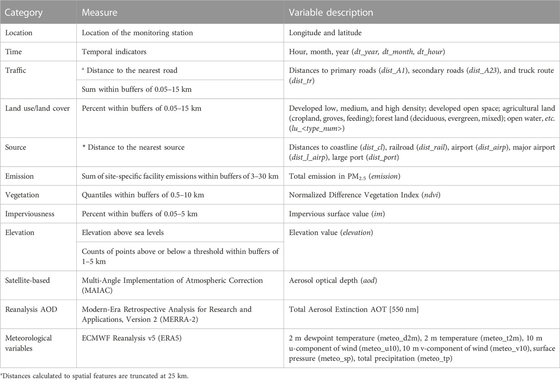
TABLE 2. Geographical covariates.
To ensure the geographic covariates included in the models provide sufficiently useful information, we apply the following criteria to filter out variables when 1) >80% of monitors had the same value, 2) >2% of observations were more than five standard deviations (SDs) away from the mean, 3) the SD of the distribution of values at cohort participant residences was more than five times the SD of the distribution of values at monitor locations, and 4) the maximum value of a percentage variable was 10% among all monitors. In addition, we removed correlated and redundant variables to avoid model overfitting by optimizing the selection of specific predictor variables with varying buffer sizes (e.g., land use type and NDVI). Specifically, using the complete set of candidate predictors, we ran an initial Random Forest model and computed variable importance scores (VIS). We then chose the buffer size for each spatial predictor as the most optimal predictor based on VIS ranking.
MAIAC AOD has a high spatial resolution of ∼1 km with local spatial variation but is only available twice daily in the afternoon. To fill the gaps of hourly AOD, we followed the work of MERRA-2 AOD downscaling using elevation. The MERRA-2 aerosol reanalysis product is simulated by Goddard Chemistry Aerosol Radiation and Transport (GOCART) coupled with the Goddard Earth Observing System, Version 5 (GEOS-5) atmospheric general circulation model (Molod et al., 2015; Gelaro et al., 2017; Randles et al., 2017). However, the 0.5 o MERRA-2 AOD might not appropriately represent the spatial distribution of aerosol loading, especially over highly polluted areas with large gradients of AOD. Therefore, MERRA-2 AOD is further downscaled from 0.5o to 1 km based on elevation (Sengupta et al., 2018) and used to fill the gaps of hourly AOD when MAIAC AOD has missing information.
We employed Automated Machine Learning (AutoML) to capture the non-linear relationships between geographic covariates and air pollutant concentrations (Breiman, 2001), as illustrated in Figure 2. AutoML is the process of automating various aspects of the machine learning workflow, including data preparation, feature engineering, model selection, hyperparameter tuning, and model deployment. AutoML is typically used to address the following challenges in machine learning: 1) time-consuming and repetitive tasks and 2) hyperparameter tuning. We used one of the AutoML open-source toolkits, Auto-sklearn (Feurer et al., 2022; 2015), built on top of the scikit-learn machine learning library. Auto-sklearn uses a Bayesian optimization approach to search the hyperparameter space efficiently and identify the best-performing model for a given dataset. It employs ensemble methods to combine multiple models and enhance the overall performance.
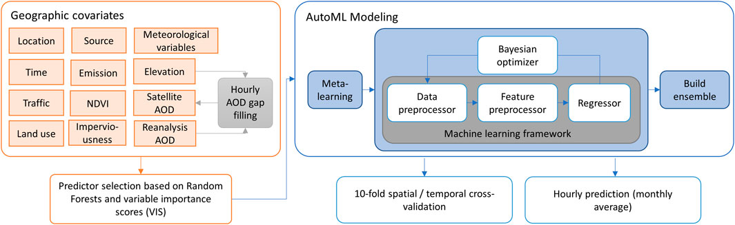
FIGURE 2. AutoML land use regression model architecture.
During the model training for the new dataset, the meta-features of the new dataset are first computed and used to compare it to the reference datasets in the meta-feature space by comparing datasets using the L1 distance, which measures the absolute differences between the meta-features of the new dataset and the reference datasets. The reference datasets are then ranked based on their distance to the new dataset, and the top 25 nearest reference datasets are selected. The hyperparameters that gave the best performance on these datasets are then used to instantiate the Bayesian optimizer for the new dataset. This helps to reduce the search space for hyperparameters and can lead to faster and more efficient hyperparameter optimization.
To test the model’s overall capability, we conducted a 10-fold cross-validation and computed the root mean squared error (RMSE) and R2 (coefficient of determination) of the observed versus fitted values to assess the model’s predictive accuracy. In addition, we evaluated the LUR results in the spatial and temporal dimensions using spatial cross-validation and temporal cross-validation separately, which involves partitioning the data into subsets and using one subset for training the LUR model and the remaining subset for testing. These evaluation metrics can help assess the ability of the LUR model to generalize to data in other spatial regions and new time periods and to estimate the spatial and temporal variations of air pollution exposure.
Quantifying human exposure to air pollution depends on two factors: 1) the population living within the area and 2) the air pollution concentration to which they are exposed. Combining the two factors, existing studies utilized population-weighted annual average concentration as a score to estimate population exposures, thus giving greater weight to the air pollution exposure where most people live (Reis et al., 2018). The population-weighted exposure is generally defined as
To account for human mobility in the estimation of PM2.5 exposure, we used the publicly available human mobility dataset SafeGraph to calculate population-weighted exposure. Specifically, we used the SafeGraph Patterns data product, which contains mobility patterns from approximately 47 million (around 10% of) mobile devices in the United States (Squire, 2019; Coston et al., 2021). The monthly Patterns data product used in this study provides anonymized counts of how many people visit commercial points of interest (POIs) each month, which can be divided by the visitor’s home census block group (CBG). Note that the term “visitors” is not used in the conventional sense to distinguish between residents and non-residents. Rather, it refers to individuals visiting Points of Interest (POIs) in a specific area. This can be helpful for understanding how mobility patterns may impact exposure to air pollution, as people who spend more time in areas with higher pollution concentrations may be at greater risk of exposure. Since the data is aggregated into monthly patterns, home CBG information is not directly linked to a specific device, differentiating SafeGraph mobility data from other individual mobility tracking datasets, such as Call Detailed Records (CDR) or mobility survey datasets. Therefore, patterns are aggregated and approximated as community-level mobility instead of individual-based. For the visitor population, we used the ‘popularity by hour’ field from SafeGraph data for each point of interest (POI) and aggregated the values into each CBG.
Based on the estimated population, a mobility-based exposure (MBE) is calculated by matching visit locations with PM2.5 concentrations estimated from the AutoML-LUR model. Specifically, MBE is calculated as follows:
where
The model prediction performance varied temporally and spatially (Table 3). Replacing EPA data with PurpleAir data to train AutoML-LUR models resulted in significant decreases in the root mean squared error (RMSE), with a decrease of 0.51 μg/m3 (SD = 0.22 μg/m3) on average. In addition, using EPA + PurpleAir data to train AutoML-LUR models also resulted in significant decreases in RMSE compared to using EPA data only, with a decrease of 0.32 μg/m3 (SD = 0.26 μg/m3) on average. However, diverging patterns of RMSE and R2values are observed across different regions. For example, in regions such as Chicago and Houston, lower RMSE and higher R2 values were observed when only PurpleAir sensor data were used. However, in other regions such as Los Angeles, models trained on combined EPA and PurpleAir data outperformed those using only PurpleAir data. Several underlying factors may explain these observed variations. Firstly, the geographical placement of sensors is a significant determinant. PurpleAir sensors, predominantly purchased by private residents, are often situated within residential areas. In contrast, EPA monitors are strategically positioned near pollution emission sources or within areas characterized by particular land use types. Consequently, the heightened performance of models in regions using solely PurpleAir data (such as Chicago) could be attributed to their greater sensitivity in capturing the air quality variations within residential environments. Secondly, the spatial distribution and density of sensors is another potential influencer. In the regions where combined sensor data yielded higher performance (such as Los Angeles), the heterogeneous sensor locations and increased sensor density could be contributing factors. The amalgamation of data from both types of sensors provides a broader representation of air quality variations across distinct land uses and proximities to emission sources. Furthermore, the level of congruity between readings from different sensors may impact model performance. As supported by Figure 1, PurpleAir sensors demonstrate greater consistency among themselves compared to their consistency with EPA monitors, thus resulting in enhanced performance when solely PurpleAir data is employed.
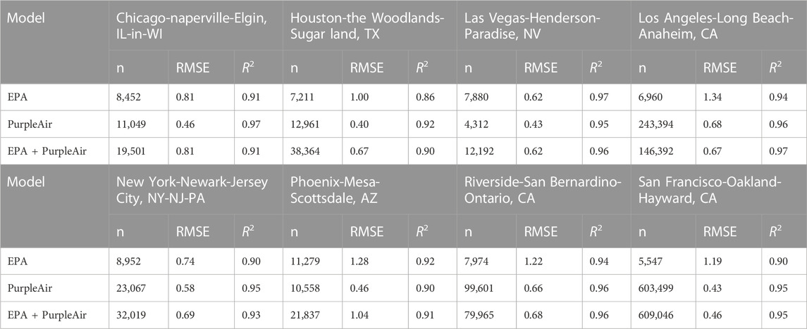
TABLE 3. Model performances–Auto-ML.
The trained models allow the mapping of pollutant concentrations in the eight CBSAs. Local variations of PM2.5 concentrations also vary by the input and can be significantly different among models (Figures 3A–C). AutoML-LUR models trained with EPA data tend to produce a higher concentration of PM2.5 than models trained with PurpleAir data. Models trained with EPA + PurpleAir data showed higher spatial variance than the other two models, with high PM2.5 concentrations varying spatially according to the observation used to train the AutoML-LUR model. Examples of predicting PM2.5 for different hours in January 2021 in Los Angeles are shown in Figure 3D–G).

FIGURE 3. (A–C) AutoML-LUR results for PM2.5 concentrations at Local Hour 0 January 2021 from models trained using EPA data, PurpleAir data, and EPA + PurpleAir data (B–G) Hourly estimates of PM2.5 concentrations in Los Angeles for January 2021. Unit: µg/m.3.
Figure 4 demonstrates the monthly trends of PM2.5 predictions in the target CBSAs. Most CBSAs show a seasonal trend of PM2.5 concentrations, but the levels of PM2.5 concentrations vary significantly depending on location. For example, the levels of PM2.5 concentrations tend to be the highest during the winter months in Los Angeles, primarily because of the increased emission and weather patterns in winter months, such as temperature inversions which can trap pollutants near the ground leading to higher PM2.5 level (Wallace et al., 2010). On the other hand, PM2.5 concentrations increased during the summer months in San Francisco, primarily because of natural sources such as wildfires. Some other CBSAs have higher PM2.5 concentrations during summer months due to a variety of factors, such as increased heat and sunlight, which can lead to the formation of ground-level ozone, a major component of smog. Other factors that may contribute to the high PM2.5 levels during summer include increased use of air conditioning and wildfires, which can release particles into the air.

FIGURE 4. Boxplots of monthly predictions in 2021 for AutoML-LUR models for each CBSA. Unit: µg/m.3.
Permutation feature importance was calculated to represent the increase in the prediction error of the model after we permuted feature’s values, which breaks the relationship between the feature and the true outcome (Fisher et al., 2019). Analyses of feature importance revealed the key factors that were spatially correlated with PM2.5 concentrations (Figure 5). Spatially aggregated feature importance scores showed that satellite AOD, temporal indicators, and meteorological variables were highly correlated with PM2.5 concentrations (Figure 5A). City-wise feature important scores reflect city-wide features most relevant to air pollutant concentrations. In most CBSAs, satellite AOD, meteorological variables, temporal indicators, NDVI, and land use remain highly correlated with PM2.5 concentrations. Figure 5B–I provides a decomposed analysis for each CBSA. Spatial heterogeneity is observed regarding the CBSA’s most relevant sources of PM2.5 other than AOD and meteorological conditions (e.g., distance to large airports for Chicago; imperviousness for Houston; nearby primary road length for Las Vegas; emission for Los Angeles, New York and Riverside; distance to coastline for New York, Riverside, and San Francisco; elevation for Phoenix and San Francisco).
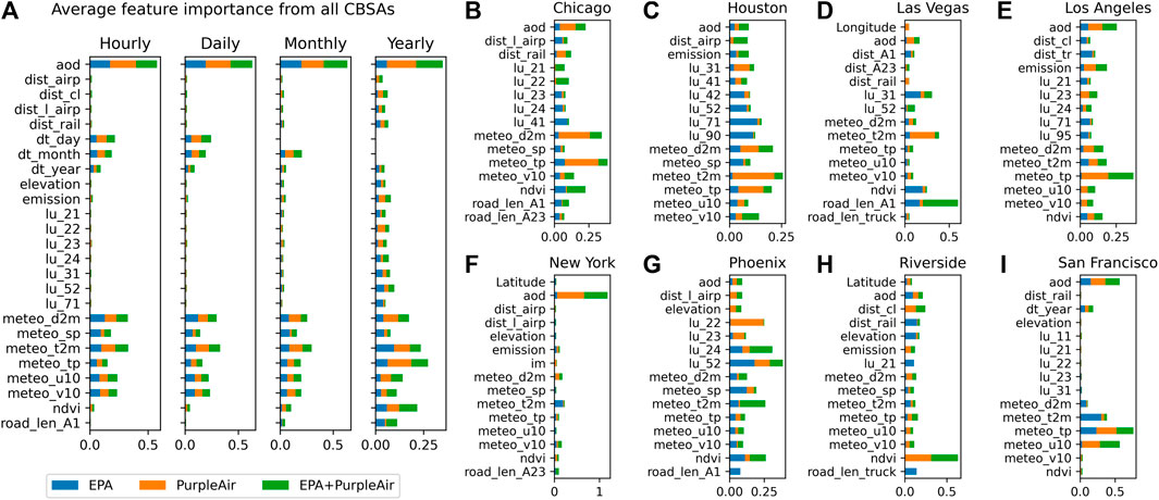
FIGURE 5. (A) Top 20 feature importance scores averaged from all eight CBSAs for all time scales, and (B–I) Top 15 feature importance scores separately for each CBSA for the yearly models. x-axes: feature importance scores, y-axes: feature abbreviations.
Mobility-based exposure (MWE) for each census block group was calculated to analyze visitor exposure to air pollution, which was shown to vary significantly in terms of spatial distribution and temporal variation. Spatial patterns of MWE reveal hotspots of high visitor number weighted exposure to PM2.5 and places where visitors are less exposed to this pollutant. For Los Angeles, the highest MWE values are found in areas near major transportation hubs and business districts, such as the Los Angeles International Airport, the Port of Los Angeles and Port of Long Beach, and Hollywood (Figure 6A). These values can vary over the time of the day and month of the year, as illustrated in the enlarged areas (Figures 6B–F). The months chosen to illustrate the temporal variation in Figures 6B–F were selected to represent different seasons throughout the year, to capture the potential seasonal differences in PM2.5 exposure and visitor patterns in various areas of Los Angeles. These months also provide a comprehensive picture of visitor exposure to PM2.5 throughout the year. Most of the CBGs demonstrate a relatively consistent pattern of MWE throughout the day, which might result from the levels of PM2.5 or a relatively low number of visitors throughout the day. CBGs that are significantly deviating from the general temporal patterns show clear diurnal trends. One typical trend is that MWE increases during the day, peaking in the late morning to early afternoon as people arrive for work or other activities. MWE declines in the late afternoon and evening as people finish their activities and return home or to their lodging. Another typical trend is that MWE remains high at night and decreases during the day, which might result from high PM2.5 concentrations or high visitor numbers at night.
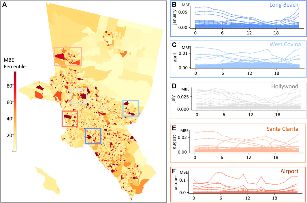
FIGURE 6. (A) Spatial patterns of percentiles for the annual average MBE for Los Angeles (B–F) Zoomed in high MBE-valued regions and their hourly MBE changes during a selected month. Each line corresponds to a particular CBG.
MWE to PM2.5 is a measure of the average exposure of visitors to a particular area, considering both the concentration of PM2.5 in the air and the number of visitors present in the area. Supposing either of these factors is exceptionally high, the MWE value may appear as a hotspot within the region, indicating a potential area of concern for air quality and public health. However, it is important to note that a high MWE value on its own does not necessarily indicate significant exposure risks without examining both factors separately. For example, a high MWE value may be due to a high number of visitors in an area with relatively low PM2.5 concentrations (Figure 7A. Airport), or it could be due to a relatively low number of visitors in an area with very high PM2.5 concentrations (Figure 7B. Long Beach). In the first case, the risk of exposure to PM2.5 for visitors may be relatively low, while in the second case, the risk may be much higher. Therefore, examining the visitor numbers and PM2.5 concentrations separately is important to get a complete picture of potential exposure risks. This can help policymakers and public health officials develop targeted strategies to reduce exposure to PM2.5 and improve air quality in areas with high levels of visitor activity.
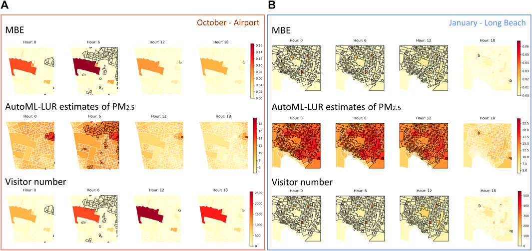
FIGURE 7. Spatial patterns of MBE, AutoML-LUR estimates of PM2.5, and visitor numbers at different hours of a particular month for two subset regions in Los Angeles. CBGs with black boundaries represent AutoML-LUR estimates of PM2.5 higher than 12 μg/m3.
This research aimed to improve the accuracy of LUR models for urban air pollution exposure assessments by integrating AutoML and low-cost sensor networks. AutoML-LUR models were developed and tested in eight CBSAs in the US, and results showed that integrating PurpleAir data into the model improves their prediction performance, particularly in areas with scarce regulatory monitoring stations. However, models developed using both EPA and PurpleAir data showed higher variance across different CBSAs compared to those developed using only EPA data. Based on the AutoML-LUR models, feature importance was calculated to identify the key factors that are spatially correlated with PM2.5 concentrations. Results showed that in most CBSAs, satellite AOD, meteorological variables, temporal indicators, NDVI, and land use remain highly correlated with PM2.5 concentrations, while the other important features vary in different spatial regions. Additionally, the study calculated mobility-based exposure (MBE) to PM2.5 using aggregated human mobility data from SafeGraph to understand how these exposures vary spatially and temporally. The results showed that areas with higher MBE values are found in neighborhoods with a high number of major transportation hubs, industries, and businesses, which might result from a high PM2.5 concentration or large visitor numbers.
This study has several implications for environmental science and public health. First, integrating AutoML and low-cost sensor networks can improve the accuracy of LUR models for air pollution exposure assessments, which provides more precise and reliable data for public health studies and decision-making. Second, spatial heterogeneity and temporal variations in the key factors relevant to PM2.5 concentrations can be used to develop more effective strategies to reduce exposure to air pollution and improve public health. Public health officials and policymakers can use the outcome of this research to 1) develop targeted interventions, such as reducing emissions from major transportation hubs or promoting green spaces in areas with high PM2.5 concentrations, at a finer temporal interval; 2) identify areas where vulnerable populations may be at higher risk of exposure to air pollution, 3) promote the use of low-cost sensor networks to improve air quality monitoring in their communities, and 4) support evidence-based decision-making on issues such as air quality regulations, land use planning, and transportation policies using AutoML algorithms to integrate multiple sources of data.
There are several limitations of this study. First, the AutoML-LUR method relies heavily on the data availability and accuracy of air quality monitors. Incorporating PurpleAir measurements improved overall accuracy, but their data quality needs screening and calibration. Limited sensor distribution in some areas can result in higher uncertainty in the predictions made by the model for these areas. Second, models with higher temporal resolution may suffer from higher uncertainty due to the greater complexity of the model and the need to account for more variables. This can be particularly challenging in estimating PM2.5, which can dramatically vary event by event due to scenarios such as wildfires, fireworks, and dust storms. To address this issue, it may be necessary to develop event-specific models or use more sophisticated models incorporating pattern shifts due to these events (Yu et al., 2022). Third, SafeGraph data represents approximate mobility patterns for a community rather than individual people, limiting its representativeness in estimating the visitor population for each census block group. Using data from the American Community Survey (ACS) can supplement the mobility data and improve representativeness. Although ACS is conducted annually and does not provide real-time individual-level data, it can provide valuable context to the SafeGraph mobility data. For example, using the ACS data, we can infer demographic and socioeconomic characteristics of individuals such as income, education level, race/ethnicity, and age. By combining this information with SafeGraph data, we can enhance our understanding of who is visiting these locations and thus refine our exposure estimates by accounting for these demographics, which can influence exposure susceptibility and behavior. Lastly, SafeGraph employs data suppression techniques to protect individual privacy. This can result in underrepresentation or inaccuracies in visitation data for locations with low foot traffic or device count, potentially impacting the accuracy of our exposure estimates in these areas (Hu et al., 2021). Future research should explore methods to counteract the effects of data suppression and investigate the specific impacts of these techniques on exposure estimates.
Future studies should address several challenges to improve our understanding of human exposure to air pollution and its impact on public health. First, socio-economic disparities in human exposure to PM2.5 can be further analyzed to identify and address potential health inequities. Understanding how different groups are affected by air pollution, based on their socioeconomic and demographic characteristics, is essential for public health planning and policy-making. Second, exposure models integrating numerical and human mobility simulation have been valuable tools for understanding and predicting human exposure to air pollution and other environmental hazards. These simulations involve 1) physical processes that govern the movement and dispersion of pollutants in the environment and 2) the movements and activities of individuals to estimate their exposure to these pollutants. Using data on human mobility, such as that provided by SafeGraph, can help to improve the accuracy and reliability of these models by providing more detailed and realistic information on the movements and activities of individuals. By incorporating this information into the model, it may be possible to predict and understand how people are exposed to air pollution more accurately. Finally, follow-up research should investigate indoor air quality exposure and compare it to outdoor exposure in this study. Understanding the differences between indoor and outdoor exposure and their effects on public health outcomes can help to inform strategies for improving air quality and reducing exposure to pollutants.
The raw data that support the findings of this study are available from the corresponding author upon reasonable request.
MY: data curation, conceptualization, methodology, code implementation, experiment, result analysis, paper writing SZ: conceptualization, paper review and editing KZ: conceptualization, paper writing, paper review and editing JY: data curation, methodology, paper review and editing MV: code implementation, experiment JM: code implementation, experiment. All authors contributed to the article and approved the submitted version.
This research is funded by the Miller Faculty Fellow Award from the College of Earth and Mineral Sciences at Penn State University.
The authors declare that the research was conducted in the absence of any commercial or financial relationships that could be construed as a potential conflict of interest.
All claims expressed in this article are solely those of the authors and do not necessarily represent those of their affiliated organizations, or those of the publisher, the editors and the reviewers. Any product that may be evaluated in this article, or claim that may be made by its manufacturer, is not guaranteed or endorsed by the publisher.
Ardon-Dryer, K., Dryer, Y., Williams, J. N., and Moghimi, N. (2020). Measurements of PM2.5 with PurpleAir under atmospheric conditions. Atmos. Meas. Tech. 13, 5441–5458. doi:10.5194/amt-13-5441-2020
Barkjohn, K. K., Gantt, B., and Clements, A. L. (2021). Development and application of a United States-wide correction for PM2.5 data collected with the PurpleAir sensor. Atmos. Meas. Tech. 14, 4617–4637. doi:10.5194/amt-14-4617-2021
Beelen, R., Raaschou-Nielsen, O., Stafoggia, M., Andersen, Z. J., Weinmayr, G., Hoffmann, B., et al. (2014). Effects of long-term exposure to air pollution on natural-cause mortality: An analysis of 22 European cohorts within the multicentre ESCAPE project. Lancet 383, 785–795. doi:10.1016/S0140-6736(13)62158-3
Bi, J., Carmona, N., Blanco, M. N., Gassett, A. J., Seto, E., Szpiro, A. A., et al. (2022). Publicly available low-cost sensor measurements for PM2.5 exposure modeling: Guidance for monitor deployment and data selection. Environ. Int. 158, 106897. doi:10.1016/j.envint.2021.106897
Black, C., Tesfaigzi, Y., Bassein, J. A., and Miller, L. A. (2017). Wildfire smoke exposure and human health: Significant gaps in research for a growing public health issue. Environ. Toxicol. Pharmacol. 55, 186–195. doi:10.1016/j.etap.2017.08.022
Butt, E. W., Turnock, S. T., Rigby, R., Reddington, C. L., Yoshioka, M., Johnson, J. S., et al. (2017). Global and regional trends in particulate air pollution and attributable health burden over the past 50 years. Environ. Res. Lett. 12, 104017. doi:10.1088/1748-9326/aa87be
Canha, N., Diapouli, E., and Almeida, S. M. (2021). Integrated human exposure to air pollution. Int. J. Environ. Res. Public Health 18, 2233. doi:10.3390/ijerph18052233
Caubel, J. J., Cados, T. E., Preble, C. V., and Kirchstetter, T. W. (2019). A distributed network of 100 black carbon sensors for 100 Days of air quality monitoring in west oakland, California. Environ. Sci. Technol. 53, 7564–7573. doi:10.1021/acs.est.9b00282
Coker, E. S., Amegah, A. K., Mwebaze, E., Ssematimba, J., and Bainomugisha, E. (2021). A land use regression model using machine learning and locally developed low cost particulate matter sensors in Uganda. Environ. Res. 199, 111352. doi:10.1016/j.envres.2021.111352
Coston, A., Guha, N., Ouyang, D., Lu, L., Chouldechova, A., and Ho, D. E. (2021). “Leveraging administrative data for bias audits: Assessing disparate coverage with mobility data for COVID-19 policy,” in Proceedings of the 2021 ACM conference on fairness, accountability, and transparency, 173–184. doi:10.1145/3442188.3445881
de Souza, J. B., Reisen, V. A., Franco, G. C., Ispány, M., Bondon, P., and Santos, J. M. (2018). Generalized additive models with principal component analysis: An application to time series of respiratory disease and air pollution data. J. R. Stat. Soc. Ser. C Appl. Statistics) 67, 453–480. doi:10.1111/rssc.12239
Feurer, M., Eggensperger, K., Falkner, S., Lindauer, M., and Hutter, F. (2022). Auto-sklearn 2.0: Hands-free AutoML via meta-learning.
Feurer, M., Klein, A., Eggensperger, K., Springenberg, J., Blum, M., and Hutter, F. (2015). “Efficient and robust automated machine learning,” in Advances in neural information processing systems (Red Hook, NY: Curran Associates, Inc).
Fisher, A., Rudin, C., and Dominici, F. (2019). All models are wrong, but many are useful: Learning a variable’s importance by studying an entire class of prediction models simultaneously. doi:10.48550/arXiv.1801.01489
Fowlie, M., Walker, R., and Wooley, D. (2020). Climate policy, environmental justice, and local air pollution. Brookings Econ. Stud. 27.
Gelaro, R., McCarty, W., Suárez, M. J., Todling, R., Molod, A., Takacs, L., et al. (2017). The modern-era retrospective analysis for research and applications, version 2 (MERRA-2). J. Clim. 30, 5419–5454. doi:10.1175/JCLI-D-16-0758.1
Gupta, P., Doraiswamy, P., Levy, R., Pikelnaya, O., Maibach, J., Feenstra, B., et al. (2018). Impact of California fires on local and regional air quality: The role of a low-cost sensor network and satellite observations. GeoHealth 2, 172–181. doi:10.1029/2018GH000136
Han, Y., Lam, J. C. K., Li, V. O. K., and Zhang, Q. (2022). A domain-specific bayesian deep-learning approach for air pollution forecast. IEEE Trans. Big Data 8, 1034–1046. doi:10.1109/TBDATA.2020.3005368
Hoek, G., Beelen, R., de Hoogh, K., Vienneau, D., Gulliver, J., Fischer, P., et al. (2008). A review of land-use regression models to assess spatial variation of outdoor air pollution. Atmos. Environ. 42, 7561–7578. doi:10.1016/j.atmosenv.2008.05.057
Hu, T., Wang, S., She, B., Zhang, M., Huang, X., Cui, Y., et al. (2021). Human mobility data in the COVID-19 pandemic: Characteristics, applications, and challenges. Int. J. Digital Earth 14, 1126–1147. doi:10.1080/17538947.2021.1952324
Jain, S., Presto, A. A., and Zimmerman, N. (2021). Spatial modeling of daily PM2.5, NO2, and CO concentrations measured by a low-cost sensor network: Comparison of linear, machine learning, and hybrid land use models. Environ. Sci. Technol. 55, 8631–8641. doi:10.1021/acs.est.1c02653
Jbaily, A., Zhou, X., Liu, J., Lee, T.-H., Kamareddine, L., Verguet, S., et al. (2022). Air pollution exposure disparities across US population and income groups. Nature 601, 228–233. doi:10.1038/s41586-021-04190-y
Keller, J. P., Olives, C., Kim, S.-Y., Sheppard, L., Sampson, P. D., Szpiro, A. A., et al. (2015). A unified spatiotemporal modeling approach for predicting concentrations of multiple air pollutants in the multi-ethnic study of Atherosclerosis and air pollution. Environ. Health Perspect. 123, 301–309. doi:10.1289/ehp.1408145
Kelly, K. E., Xing, W. W., Sayahi, T., Mitchell, L., Becnel, T., Gaillardon, P.-E., et al. (2021). Community-based measurements reveal unseen differences during air pollution episodes. Environ. Sci. Technol. 55, 120–128. doi:10.1021/acs.est.0c02341
Kirwa, K., Szpiro, A. A., Sheppard, L., Sampson, P. D., Wang, M., Keller, J. P., et al. (2021). Fine-scale air pollution models for epidemiologic research: Insights from approaches developed in the multi-ethnic study of Atherosclerosis and air pollution (MESA air). Curr. Envir Health Rpt 8, 113–126. doi:10.1007/s40572-021-00310-y
Lee, M., Brauer, M., Wong, P., Tang, R., Tsui, T. H., Choi, C., et al. (2017). Land use regression modelling of air pollution in high density high rise cities: A case study in Hong Kong. Sci. Total Environ. 592, 306–315. doi:10.1016/j.scitotenv.2017.03.094
Li, L., Girguis, M., Lurmann, F., Pavlovic, N., McClure, C., Franklin, M., et al. (2020). Ensemble-based deep learning for estimating PM2.5 over California with multisource big data including wildfire smoke. Environ. Int. 145, 106143. doi:10.1016/j.envint.2020.106143
Lu, T., Bechle, M. J., Wan, Y., Presto, A. A., and Hankey, S. (2022). Using crowd-sourced low-cost sensors in a land use regression of PM2.5 in 6 US cities. Air Qual. Atmos. Health 15, 667–678. doi:10.1007/s11869-022-01162-7
Lu, Y., Giuliano, G., and Habre, R. (2021). Estimating hourly PM2.5 concentrations at the neighborhood scale using a low-cost air sensor network: A Los Angeles case study. Environ. Res. 195, 110653. doi:10.1016/j.envres.2020.110653
Ma, X., Longley, I., Salmond, J., and Gao, J. (2020). PyLUR: Efficient software for land use regression modeling the spatial distribution of air pollutants using GDAL/OGR library in Python. Front. Environ. Sci. Eng. 14, 44. doi:10.1007/s11783-020-1221-5
Masiol, M., Zíková, N., Chalupa, D. C., Rich, D. Q., Ferro, A. R., and Hopke, P. K. (2018). Hourly land-use regression models based on low-cost PM monitor data. Environ. Res. 167, 7–14. doi:10.1016/j.envres.2018.06.052
McDuffie, E. E., Martin, R. V., Spadaro, J. V., Burnett, R., Smith, S. J., O’Rourke, P., et al. (2021). Source sector and fuel contributions to ambient PM2.5 and attributable mortality across multiple spatial scales. Nat. Commun. 12, 3594. doi:10.1038/s41467-021-23853-y
Meng, X., Chen, L., Cai, J., Zou, B., Wu, C.-F., Fu, Q., et al. (2015). A land use regression model for estimating the NO2 concentration in shanghai, China. Environ. Res. 137, 308–315. doi:10.1016/j.envres.2015.01.003
Molod, A., Takacs, L., Suarez, M., and Bacmeister, J. (2015). Development of the GEOS-5 atmospheric general circulation model: Evolution from MERRA to MERRA2. Geosci. Model. Dev. 8, 1339–1356. doi:10.5194/gmd-8-1339-2015
Morley, D. W., and Gulliver, J. (2018). A land use regression variable generation, modelling and prediction tool for air pollution exposure assessment. Environ. Model. Softw. 105, 17–23. doi:10.1016/j.envsoft.2018.03.030
Muttoo, S., Ramsay, L., Brunekreef, B., Beelen, R., Meliefste, K., and Naidoo, R. N. (2018). Land use regression modelling estimating nitrogen oxides exposure in industrial south Durban, South Africa. Sci. Total Environ. 610– 611, 1439–1447. doi:10.1016/j.scitotenv.2017.07.278
Nyhan, M., Grauwin, S., Britter, R., Misstear, B., McNabola, A., Laden, F., et al. (2016). “Exposure track”—the impact of mobile-device-based mobility patterns on quantifying population exposure to air pollution. Environ. Sci. Technol. 50, 9671–9681. doi:10.1021/acs.est.6b02385
Nyhan, M. M., Kloog, I., Britter, R., Ratti, C., and Koutrakis, P. (2019). Quantifying population exposure to air pollution using individual mobility patterns inferred from mobile phone data. J. Expo. Sci. Environ. Epidemiol. 29, 238–247. doi:10.1038/s41370-018-0038-9
Orun, A., Elizondo, D., Goodyer, E., and Paluszczyszyn, D. (2018). Use of Bayesian inference method to model vehicular air pollution in local urban areas. Transp. Res. Part D Transp. Environ. 63, 236–243. doi:10.1016/j.trd.2018.05.009
Raffuse, S., Sullivan, D., McCarthy, M., Penfold, B., and Hafner, H. (2007). Ambient air monitoring network assessment guidance, analytical techniques for technical assessments of ambient air monitoring networks. Retrieved July 20, 2007).
Randles, C. A., Silva, A. M. da, Buchard, V., Colarco, P. R., Darmenov, A., Govindaraju, R., et al. (2017). The MERRA-2 aerosol reanalysis, 1980 onward. Part I: System description and data assimilation evaluation. J. Clim. 30, 6823–6850. doi:10.1175/JCLI-D-16-0609.1
Ravindra, K., Rattan, P., Mor, S., and Aggarwal, A. N. (2019). Generalized additive models: Building evidence of air pollution, climate change and human health. Environ. Int. 132, 104987. doi:10.1016/j.envint.2019.104987
Reid, C. E., Brauer, M., Johnston, F. H., Jerrett, M., Balmes, J. R., and Elliott, C. T. (2016). Critical review of health impacts of wildfire smoke exposure. Environ. Health Perspect. 124, 1334–1343. doi:10.1289/ehp.1409277
Reis, S., Liška, T., Vieno, M., Carnell, E. J., Beck, R., Clemens, T., et al. (2018). The influence of residential and workday population mobility on exposure to air pollution in the UK. Environ. Int. 121, 803–813. doi:10.1016/j.envint.2018.10.005
Ren, X., Mi, Z., and Georgopoulos, P. G. (2020). Comparison of Machine Learning and Land Use Regression for fine scale spatiotemporal estimation of ambient air pollution: Modeling ozone concentrations across the contiguous United States. Environ. Int. 142, 105827. doi:10.1016/j.envint.2020.105827
Roberts, S., and Martin, M. (2005). A critical assessment of shrinkage-based regression approaches for estimating the adverse health effects of multiple air pollutants. Atmos. Environ. 39, 6223–6230. doi:10.1016/j.atmosenv.2005.07.004
Sengupta, M., Xie, Y., Lopez, A., Habte, A., Maclaurin, G., and Shelby, J. (2018). The national solar radiation data base (NSRDB). Renew. Sustain. Energy Rev. 89, 51–60. doi:10.1016/j.rser.2018.03.003
Shaddick, G., Thomas, M. L., Mudu, P., Ruggeri, G., and Gumy, S. (2020). Half the world’s population are exposed to increasing air pollution. npj Clim. Atmos. Sci. 3, 23. doi:10.1038/s41612-020-0124-2
Squire, R. (2019). What about bias in the SafeGraph dataset? [WWW Document]. URL Available at: https://www.safegraph.com/blog/what-about-bias-in-the-safegraph-dataset (accessed 13 7, 22).
Sun, X., Zhao, T., Bai, Y., Kong, S., Zheng, H., Hu, W., et al. (2022). Meteorology impact on PM<sub>2.5</sub> change over a receptor region in the regional transport of air pollutants: Observational study of recent emission reductions in central China. Atmos. Chem. Phys. 22, 3579–3593. doi:10.5194/acp-22-3579-2022
Thomas, D. C., Jerrett, M., Kuenzli, N., Louis, T. A., Dominici, F., Zeger, S., et al. (2007). Bayesian model averaging in time-series studies of air pollution and mortality. J. Toxicol. Environ. Health, Part A 70, 311–315. doi:10.1080/15287390600884941
Tryner, J., L’Orange, C., Mehaffy, J., Miller-Lionberg, D., Hofstetter, J. C., Wilson, A., et al. (2020). Laboratory evaluation of low-cost PurpleAir PM monitors and in-field correction using co-located portable filter samplers. Atmos. Environ. 220, 117067. doi:10.1016/j.atmosenv.2019.117067
Wallace, J., Corr, D., and Kanaroglou, P. (2010). Topographic and spatial impacts of temperature inversions on air quality using mobile air pollution surveys. Sci. Total Environ. 408, 5086–5096. doi:10.1016/j.scitotenv.2010.06.020
Wallace, L., Bi, J., Ott, W. R., Sarnat, J., and Liu, Y. (2021). Calibration of low-cost PurpleAir outdoor monitors using an improved method of calculating PM. Atmos. Environ. 256, 118432. doi:10.1016/j.atmosenv.2021.118432
Weissert, L., Alberti, K., Miles, E., Miskell, G., Feenstra, B., Henshaw, G. S., et al. (2020). Low-cost sensor networks and land-use regression: Interpolating nitrogen dioxide concentration at high temporal and spatial resolution in Southern California. Atmos. Environ. 223, 117287. doi:10.1016/j.atmosenv.2020.117287
WHO (2022). Billions of people still breathe unhealthy air. new WHO data [WWW Document]. URL Available at: https://www.who.int/news/item/04-04-2022-billions-of-people-still-breathe-unhealthy-air-new-who-data (accessed 10 8, 22).
Wong, P.-Y., Hsu, C.-Y., Wu, J.-Y., Teo, T.-A., Huang, J.-W., Guo, H.-R., et al. (2021). Incorporating land-use regression into machine learning algorithms in estimating the spatial-temporal variation of carbon monoxide in Taiwan. Environ. Model. Softw. 139, 104996. doi:10.1016/j.envsoft.2021.104996
Yao, J., Brauer, M., Raffuse, S., and Henderson, S. B. (2018). Machine learning approach to estimate hourly exposure to fine particulate matter for urban, rural, and remote populations during wildfire seasons. Environ. Sci. Technol. 52, 13239–13249. doi:10.1021/acs.est.8b01921
Yu, M., Masrur, A., and Blaszczak-Boxe, C. (2022). Predicting hourly PM2.5 concentrations in wildfire-prone areas using a SpatioTemporal Transformer model. Sci. Total Environ. 160446, 160446. doi:10.1016/j.scitotenv.2022.160446
Yu, X., Ivey, C., Huang, Z., Gurram, S., Sivaraman, V., Shen, H., et al. (2020). Quantifying the impact of daily mobility on errors in air pollution exposure estimation using mobile phone location data. Environ. Int. 141, 105772. doi:10.1016/j.envint.2020.105772
Keywords: machine learning, land use regression, human mobility, low-cost sensors, PM2.5
Citation: Yu M, Zhang S, Zhang K, Yin J, Varela M and Miao J (2023) Developing high-resolution PM2.5 exposure models by integrating low-cost sensors, automated machine learning, and big human mobility data. Front. Environ. Sci. 11:1223160. doi: 10.3389/fenvs.2023.1223160
Received: 15 May 2023; Accepted: 03 July 2023;
Published: 13 July 2023.
Edited by:
Yichun Xie, Eastern Michigan University, United StatesReviewed by:
Xining Yang, Eastern Michigan University, United StatesCopyright © 2023 Yu, Zhang, Zhang, Yin, Varela and Miao. This is an open-access article distributed under the terms of the Creative Commons Attribution License (CC BY). The use, distribution or reproduction in other forums is permitted, provided the original author(s) and the copyright owner(s) are credited and that the original publication in this journal is cited, in accordance with accepted academic practice. No use, distribution or reproduction is permitted which does not comply with these terms.
*Correspondence: Manzhu Yu, bXF5NTE5OEBwc3UuZWR1
Disclaimer: All claims expressed in this article are solely those of the authors and do not necessarily represent those of their affiliated organizations, or those of the publisher, the editors and the reviewers. Any product that may be evaluated in this article or claim that may be made by its manufacturer is not guaranteed or endorsed by the publisher.
Research integrity at Frontiers
Learn more about the work of our research integrity team to safeguard the quality of each article we publish.