Improving prediction accuracy for acid sulfate soil mapping by means of variable selection

Acid sulfate soils can cause environmental damage and geotechnical problems when drained or exposed to oxidizing conditions. This makes them one of the most harmful soils found in nature. In order to reduce possible damage derived from this type of soil, it is fundamental to create occurrence maps showing their localization. Nowadays, occurrence maps can be created using machine learning techniques. The accuracy of these maps depends on two factors: the dataset and the machine learning method. Previously, different machine learning methods were evaluated for acid sulfate soil mapping. To improve the precision of the acid sulfate soil probability maps, in this qualitative modeling study we have added more environmental covariates (17 in total). Since a greater number of covariates does not necessarily imply an improvement in the prediction, we have selected the most relevant environmental covariates for the classification and prediction of acid sulfate soils. For this, we have applied eleven different variable selection methods. The predictive abilities of each group of selected variables have been analyzed using Random Forest and Gradient Boosting. We show that the selection of each environmental covariate as well as the relationship between them are extremely important for an accurate prediction of acid sulfate soils. Among the variable selection methods analyzed, Random Forest stands out, as it is the one that has best selected the relevant covariates for the classification of these soils. Furthermore, the combination of two variable selection methods can improve the prediction of the model. Contrary to the general belief, a low correlation between the covariates does not guarantee a good performance of the model. In general, Random Forest has given better results in the prediction than Gradient Boosting. From the best results obtained, an acid sulfate soils occurrence map has been created. Compared with previous studies in the same area, variable selection has improved the accuracy by 15%–17% for the models based on Random Forest. The present study confirms the importance of variable selection for the prediction of acid sulfate soils.

1 Introduction

In general terms, soils that present sulfidic materials in their composition and a drop or possible drop in their pH values below 4 are considered acid sulfate (AS) soils (Pons, 1973). The drop in pH values is a consequence of the oxidation of sulfidic materials. The oxidation process is often initiated by drainage of the soils in agriculture or forestry. A decrease of the soil-pH below 4 generates acidification of the soil and mobilization of several metals, and ultimately leaching of acidity and metals from the soil through subsurface drainpipes and ditches (Åström and Björklund, 1997; Österholm and Åström, 2002; Roos and Åström, 2006). Therefore, the occurrence of AS soils can lead to the deterioration of stream waters, which may cause severe ecological damages (e.g., fish kills (Hudd, 2000; Urho, 2002)), as well as problems in agriculture and its productivity (Palko, 1994) or in infrastructures with damages related to the poor stability of sulfidic sediments and corrosion of concrete and steel constructions as a consequence of the increased acidity. Due to these environmental hazards and geotechnical challenges, AS soils are considered one of the most damaging soils (Michael, 2013). For environmental authorities, mapping of AS soil occurrence is very important to identify areas with potential environmental hazards such as acidifying and metal pollution if the soil materials are disturbed. The identification (mapping) of these areas would contribute to the reduction of possible ecological damages. In infrastructure developments, the knowledge of AS soil occurrence is crucial to determine the need or not to apply measures to avoid issues related to the poor stability and corrosion of building materials, which often lead to increased building costs.

Traditional or conventional methods for mapping AS soils require a large number of soil samples as well as expert knowledge to create the maps. As a result, the mapping process can be very laborious, expensive and time consuming. Moreover, the accuracy of the resulting maps can be affected by the person who creates the map. Nowadays, digital soil mapping studies are mostly based on the use of machine learning techniques (McBratney et al., 2003). These techniques have several advantages over traditional methods. First, mapping with these methods requires fewer samples (Brus et al., 2011), leading to a much faster and less expensive process. Moreover, these techniques make the mapping process more objective and easier to replicate than traditional methods. So far, the most used machine learning techniques for AS soil mapping have been Artificial Neural Network (ANN) (Beucher et al., 2013; Beucher et al., 2015; Beucher et al., 2017), Fuzzy logic (Beucher et al., 2014) and Fuzzy k-means (Huang et al., 2014). Although there are few works, other techniques such as Convolutional Neural Network (CNN) (Estévez Nuño, 2020; Beucher et al., 2022) or Extreme Learning Machine (ELM) (Estévez et al., 2023; Akusok et al., 2023) have also been studied for the classification of AS soils. Recently, the suitability of three different machine learning methods, Random Forest (RF), Gradient Boosting (GB) and Support Vector Machines (SVM), for the classification and prediction of AS soils has been analyzed (Estévez et al., 2022). RF and GB showed high abilities for the classification and prediction of AS soils, leading to very accurate AS soil probability maps. On the contrary, it has been shown that SVM is unsuitable for mapping AS soils due to the fact that it could not adequately recognize AS soils (Estévez et al., 2022). One of the main goals of this study is to enhance the accuracy of the AS soil probability maps. For this reason, the study has been focused on improving RF and GB models using more environmental covariates. In principle, the consideration of a greater number of covariates will give more information for a better characterization of the soils. However, it should be noted that some covariates may be irrelevant or provide redundant information that could lead to a poor prediction (Hall and Holmes, 2003). Thus, the objective is to find the most relevant environmental covariates that allow the classification and prediction of the AS soils with a very high accuracy. For this, it will be essential to apply variable selection, which is one of the most important and complex topics in machine learning. Variable selection is not only fundamental for improving the prediction of the model but also to understand the relationship between the variables and the target, as well as to reduce the computing time (Guyon and Elisseeff, 2003). Variable selection has been widely used in different fields such as biomedicine and bioinformatics (Guyon et al., 2002; Saeys et al., 2007; Osl et al., 2009) or text classification problems (Forman, 2003). In soil science, the variable selection have been used for the prediction of soil organic carbon (Xiong et al., 2014; Fitzpatrick et al., 2016; Lie et al., 2016; Keskin et al., 2019), soil parent material (Heung et al., 2014), soil organic matter (Chen et al., 2022), soil depth (Tesfa et al., 2009; Camera et al., 2017; Castro Franco et al., 2017; Lu et al., 2019) and soil classes (Behrens et al., 2010; Brungard et al., 2015; Camera et al., 2017; Campos et al., 2018). So far, there are hardly any works where the selection of variables has been applied for the prediction of AS soils. In this study, the variable selection for an accurate prediction of AS soils has been analyzed in detail. As an environmental covariate can be relevant for one method but irrelevant for another (Kohavi and John, 1997), eleven different methods of variable selection have been considered. This allows the identification of the most relevant covariates for the characterization of the AS soils and their prediction. The methods used are: one Univariate Feature Selection (UFS), RF, GB, Extra Trees Classifier (ETC), Recursive Feature Elimination (RFE), Backward Selection and Pearson’s correlation. For RFE, four different methods have been considered: RF, GB, ETC and Logistic Regression (LR). The Backward Selection has been analyzed for two different methods, RF and GB. Moreover, the combination of two variable selection methods has also been studied. Once the subsets of environmental covariates were selected, their suitability for the prediction and classification of AS soils for the two machine learning methods considered for modeling, RF and GB, has been evaluated. The AS soil probability map for the study area has been created using the model and the group of environmental covariates with the highest abilities for the classification of AS soils. Finally, the extent of AS soils has been estimated based on the modeled AS soil probability map.

2 Materials and methods

2.1 Study area

The area considered for this study is Virolahti and its surroundings (1,091 km²), located in southeastern Finland (Figure 1). The land use of this region, which is part of the boreal ecosystem, is mainly forestry, agricultural lands and some urban areas. In this area, as in the rest of Finland, AS soils belong to the cryic soil temperature regime, where mean annual soil temperature 0°C–8°C and mean summer soil temperature below 15°C (Yli-Halla and Mokma, 1998). About 905 km² (83%) of the study area corresponds to the Littorina Sea maximum extent, which is the most potential area for AS soil occurrence and where the conventional AS soil mapping has been made by the Geological Survey of Finland (GTK). The geological basement is composed almost entirely of 1.66–1.60 Ga Rapakivi granite (Lehtinen et al., 1998; Geological Survey of Finland, 2021) and is covered mainly by glacial till and alluvial deposits (Haavisto-Hyvärinen and Kutvonen, 2007). The uppermost meter in the area is made up of bedrock, outcrops and block fields (57.66%), different types of soils (38.94%), water (3.19%) and a small unmapped part (0.22%). The existing soils in this area are clay (16.91%), fine sand to gravel (7.21%), till (5.85%), thick peat deposits (4.63%), gyttja (2.01%), fine-grained sediment or fine silt low humus content 2%–6% (1.21%), fine silt (1.12%), and man-made soils.

FIGURE 1

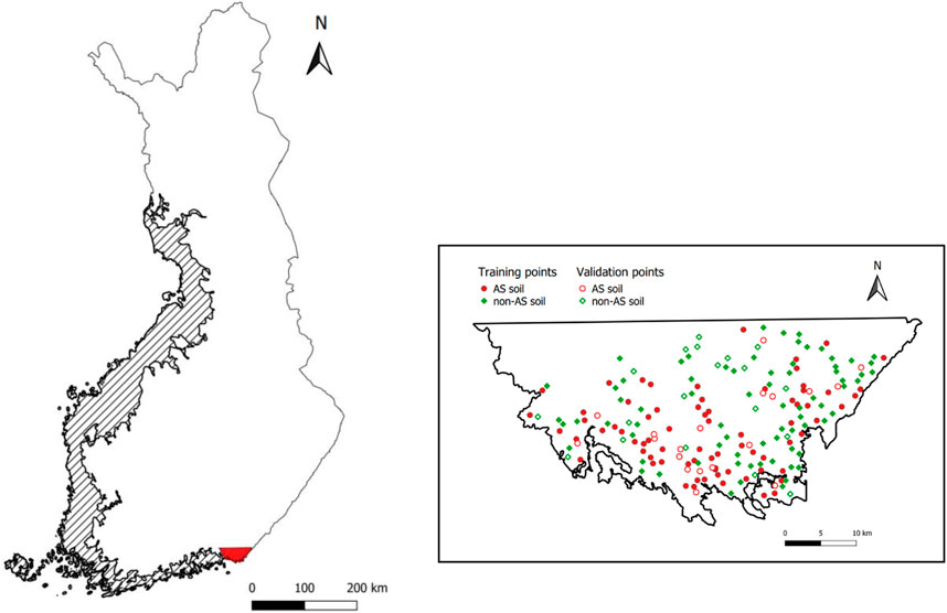
FIGURE 1. (Color online) Main figure: Location of the study area (red color) and extent of the Littorina Sea (diagonal lines). Inset: Location of the training and validation points for acid sulfate (AS) and non acid sulfate (non-AS) soils in the study area.

2.2 Soil samples

The soil cores used in this study were collected with a gouge auger down to 2–3 m depth as part of the national AS soil mapping done by GTK. The emplacement of the sampling sites was limited to the Littorina Sea maximal extent, as the majority of the Finnish AS soils are located here (Palko, 1994; Yli-Halla et al., 1999; Geological Survey of Finland, 2021). The non-statistical sampling plan used was designed to create a set of samples where the different types of soils and materials of the area were included. This was possible thanks to the consideration of all sediment classes in the quaternary geology map, different topography locations, and the electric conductivity (EC) anomalies and non-anomalies in airborne geophysical data. The sampling density during the AS soil mapping in Finland is about 1 probe/km². The exclusion of bedrock, outcrops, glacial till, man-made soils and water from the sampling, as well as the limited road network, lead to areas where the sampling density is less dense.

The classification of the soil samples or cores into AS and non-AS soils was determined by the soil-pH, which was measured in the field and/or in the laboratory after oxidation (incubation). Mineral soil materials with pH $<$ 4 and organic soil materials with pH $<$ 3 were classified as AS soils, whereas samples having pH-values above these were classified as non-AS soils, following slightly modified procedures described in (Boman et al., 2019).

2.3 Environmental covariates

In addition to soil samples, environmental data have been used in this study. The environmental covariates are raster data generated from remote sensing data. In this study, the types of remote sensing data used are LiDAR and geophysics, which originate from airborne surveys. Some environmental covariates can be fundamental to characterize different types of soils. These covariates are of several types: Quaternary geology, airborne electromagnetic or aerogeophysics data, digital elevation model and topographic or terrain data. In this study, a total of 17 environmental layers have been used (Table 2). Contrary to a previous work where only one terrain layer was considered (Estévez et al., 2022), twelve different terrain layers have been analyzed for the classification of AS soils in this study. All environmental covariates have a resolution of 50 m × 50 m and have been created using Qgis (Qgis Development Team, 2019). Furthermore, the coordinate reference system is the Finnish one (ETRS89/TM35FIN(E,N)).

2.3.1 Quaternary

The quaternary geology layer 1:200000 (Korpela and Niemelä, 1985) displays the occurrence of 12 different soil materials down to a depth of 1 m. Fine-grained gyttja bearing sediment is the most critical indicator of AS soils because they usually consist of fine-grained sediments, although in some environments it may be made up of coarse-grained soil materials (Mattbäck et al., 2017).

2.3.2 Aerogeophysics

Airborne electromagnetic data (real, imaginary and apparent resistivity components) are often useful for discovering sulfidic deposits, both in the overburden and bedrock (Airo, 2005). The aeroelectromagnetic data were collected at flight altitudes between 30 and 40 m and a line spacing of 200 m, producing a raster dataset with a resolution of 50 m. Shallow weak anomalies, that mainly relate to variations in topsoil thickness and electric conductivity, may be detected using the imaginary component whereas the real component mainly enables the detection of deeper anomalies in the bedrock, e.g., black schists (Airo and Loukola-Ruskeeniemi, 2004). The apparent resistivity is calculated from In-Phase (real) and Quadrature (imaginary) components of the measured electromagnetic field. Soil materials such as clay and gyttja have high conductivities whereas glacial till and sand have lower (Pernu, 1991).

2.3.3 Digital elevation model

A digital elevation model (DEM) is a representation of the topographic surface of the terrain. This environmental covariate will play a fundamental role in the classification of AS soils since in southern Finland, AS soils generally occurs at an elevation of less than 50 m (Palko, 1994). The DEM used in this study has been generated from the LiDAR data of the National Land Survey of Finland (NLS). The resolution of this layer is 2 m × 2 m but was down-sampled to a 50 m × 50 m which is the resolution of the aerogeophysics layers and therefore the one used in this study. The resolution change has been done in Qgis by reprojection and the resampling method used is Nearest Neighbors.

2.3.4 Terrain layers

The terrain attributes are obtained from the DEM, and widely used for classification and prediction in digital soil mapping (McBratney et al., 2003). In this study 12 terrain layers have been considered: slope, aspect, hillshade, roughness, multiresolution index of valley bottom flatness (MRVBF), multiresolution index of the ridge top flatness (MRRTF), topographic position index (TPI), terrain ruggedness index (TRI), topographic wetness index (TWI), valley depth, tangential curvature and profile curvature. In Finland, AS soils usually occur in low-relief, flat and heterogenous areas, usually with a close to zero-degree slope (Österholm et al., 2005; Becher et al., 2018). Covariates such as hillshade, slope, roughness and terrain ruggedness show this. However, it is not clear if aspect, profile curvature or tangential curvature will impact AS soil occurrence, since the direction and type of ridge do not really affect the occurrence. On the other hand, valley bottom flatness and valley depth covariates are important since they reflect depositional environments where AS soils most likely have formed. Contrary, ridge top flatness might not have that big of an impact since sulfidic sediments usually do not form on ridge tops in Finland. While topographic position index should not have that much of an impact, the wetness index is somewhat similar to valley bottom flatness and valley depth, which usually indicate waterlogged soils where AS soils are often found. Exceptions may occur in sandy areas where coarse-grained AS soils consist of littoral deposits and, where beach ridges and dunes are common (Mattbäck et al., 2017).

2.4 Machine learning methods for modeling

For the modeling, two machine learning techniques, Random Forest (RF) and Gradient Boosting (GB), have been considered. These two ensemble methods based on decision trees have shown high performance abilities for the prediction of AS soils (Estévez et al., 2022). In this work, Python (Van Rossum and Drake, 2009) has been used for all the codes and the Scikit-learn library (Pedregosa et al., 2011) for the machine learning methods. For the optimal performance of machine learning models, tuning parameters are critical (Müller and Guido, 2016). The determination of the best tuning parameters for the two machine learning models have been made with grid search and cross-validation (GridSearchCV). For more information we refer the reader to see the previous work (Estévez et al., 2022).

2.4.1 Random forest

Random Forest (RF) (Breiman, 2001) is one of the most used techniques in classification and regression problems due to its efficiency and robustness. This supervised machine learning technique combines the results of multiple decision trees to make a prediction. Each tree is created from a different sub-dataset, which has been randomly selected. For each tree, the algorithm will make a prediction that will be considered for the final prediction. This leads to a better performance than in the case of a single tree. Moreover, this technique helps to reduce overfitting. In soil science, this method has been frequently used for the prediction of soil properties (Grimm et al., 2008; Behrens et al., 2010; Wiesmeier et al., 2011; Lie et al., 2012; Schmidt et al., 2014; Veronesi and Schillaci, 2019; Azizi et al., 2022; Moradpour et al., 2023) and the classification of soils (Heung et al., 2014; Brungard et al., 2015; Gambill et al., 2016; Heung et al., 2016; Teng et al., 2018; Estévez et al., 2022).

2.4.2 Gradient boosting

For classification and regression predictions, one common supervised machine learning technique is Gradient Boosting (GB)(Friedman, 2001). This method is very efficient and can lead to predictions with very high precision if the tuning parameters are adequate. Unlike RF, GB builds the ensemble trees one by one, based on the information of the previous tree. This serial manner allows each new tree to correct the prediction errors made in the previous one. The goal of the model is to improve the final prediction. In soil science, this method has been considered to predict soil properties (Hengl et al., 2017; Sindayiheburaa et al., 2017; Tziachrisa et al., 2019) and classes (Lemercier et al., 2012; Estévez et al., 2022).

2.5 Variable selection methods

The selection of the most important covariates for the study is essential for a good classification of soils. There are covariates that do not give information to the model and can hinder the prediction (Hall and Holmes, 2003). Thus, the variable selection is fundamental for the creation of an effective predictive model. The set of the most relevant environmental covariates for the model depends on the variable selection method. Moreover, an optimal covariate set can be more appropriate for a given machine learning method than for another. In the case of classification studies, the variable selection methods are of three types: filter models, wrapper and embedded methods (Saeys et al., 2007; Kuhn and Johnson, 2013). In this study, filter models, wrapper methods and the analysis of the correlation have been considered.

2.5.1 Filter methods

The variable selection in the filter methods is independent of the machine learning techniques. This independence makes these methods computationally efficient and generally does not lead to overfitting (Saeys et al., 2007; Kuhn and Johnson, 2013). However, the set of variables selected cannot be the most suitable for a given model. Another problem is that these methods do not take into account the correlation between the variables. As a result, highly correlated variables can be selected, adding redundant information to the model.

2.5.1.1 Univariate feature selection

These methods select the most relevant features by statistical tests. Univariate refers to the fact that each variable is analyzed individually, without taking into account the relationship between the rest of the variables. Thus, the model measures the relationship of each feature with the target. The resulting values allow the selection of the most relevant variables for the target. There are several methods of univariate selection, in this work the method used is the SelectKBest from Scikit-learn (Pedregosa et al., 2011).

2.5.2 Wrapper methods

The wrapper methods use machine learning techniques for the selection of variables, which is based on the performance of the model. The most appropriate features for the model are those that improve the accuracy. In general, this makes them the best performing variable selection methods. Unlike the filter methods, the wrapper methods can cause an excessive adjustment of the results, i.e., overfitting (Kohavi and John, 1997). Furthermore, these methods require more computation time. The machine learning method used for the variable selection can be the same or different to the one used for the final modeling. In this study, we have evaluated several wrapper methods for feature selection.

2.5.2.1 Methods based on decision trees

These methods can directly give the importance of each feature for the model by means of an implemented algorithm. In this work, RF and GB have also been used for variable selection. One of the most common methods for variable selection in soil science is RF, that has been used for the prediction of soil organic carbon (Keskin et al., 2019), soil organic material (Heung et al., 2014), soil organic matter (Chen et al., 2022), soil depth (Tesfa et al., 2009; Castro Franco et al., 2017; Lu et al., 2019) or soil thickness (Li et al., 2020). In contrast, GB has only been used in variable selection for the prediction of soil depth (Lacoste et al., 2016).

In addition, another method based on decision trees has been considered for variable selection: Extra Trees Classifier (ETC).

2.5.2.1.1 Extra trees classifier

Extra trees classifier (ETC) (Geurts et al., 2006) or extremely randomized trees is an ensemble machine learning technique quite similar to RF. One difference is that in the, ETC, the decision trees are created on the whole data and not on the randomly selected data as in RF. However, the main difference in both methods is the selection of the split points in a decision tree. RF selects an optimal split point taking into account the best features, while, ETC chooses randomly the split points independently of the features. So far, ETC has never been used for classification or prediction of soil classes or properties. In this study, the method is only used for variable selection.

2.5.2.2 Backward selection

This method is based on the elimination of the irrelevant features. Initially all variables or features are considered, and in each step the least important feature for the model is eliminated. The idea is to improve the accuracy of the model. The elimination of variables will take place until the performance of the model does not improve. In this study, the machine learning techniques used for the backward selection are RF and GB. Previously, Backward Selection has been applied for the prediction of soil organic carbon (Lie et al., 2016; Veronesi and Schillaci, 2019).

2.5.2.3 Recursive feature elimination

This method is an iterative feature selection based on the elimination of the least important features (Guyon et al., 2002). This is also a backward selection, but in this case, a subset of the features with higher weight in the model is selected at once. In this way, the variable selection method is optimized due to the features selected are relevant when they are combined together. It should be noted that a feature can be relevant in presence of other features but not by itself (Guyon and Elisseeff, 2003). Recursive Feature Elimination (RFE) needs other methods to measure the weight of the features. In this study, RFE have been analyzed using four different machine learning techniques: RF, GB, ETC and Logistic Regression (LR). So far, of these methods only the RFE with RF has been used in the variable selection of environmental covariates in soil science (Brungard et al., 2015; Camera et al., 2017; Veronesi and Schillaci, 2019; Beucher et al., 2022).

2.5.2.3.1 Logistic regression

This machine learning method is widely used in binary classification problems (Müller and Guido, 2016). LR is a linear model that has been used in soil science to predict the occurrence of soil types (Giasson et al., 2006; Debella-Gilo and Etzelmüller, 2009), soil drainage classes (Campling et al., 2002) or diagnostic horizons (Jafari et al., 2012). However, LR has never been used for variable selection in soil science.

2.5.3 Correlation

Unlike previous variable selection methods, the correlation is an unsupervised method, which does not take into account the target or label. The correlation indicates the relationship between two variables, which gives information about the redundancy of the variables. In the case of highly correlated variables the information they provide is redundant (Guyon and Elisseeff, 2003). Thus, some of them can be removed without the loss of information. The correlation can be positive or negative. In the positive case, both variables increase or decrease. Whereas in the case of negative correlation, when a variable increases the other decreases. In this study, the linear correlation between features is analyzed through the Pearson correlation coefficient, whose values are in the range of −1 to 1. A correlation equal to −1 corresponds to a perfect negative correlation, while +1 is a perfect positive correlation. A coefficient equal to 0 means that there is no relationship between the features. The interpretation of the coefficient can be [0–0.2), [0.2–0.4), [0.4–0.6), [0.6–0.8) and [0.8–1], which correspond to a very low, low, moderate, high and very high correlation, respectively. The negative correlation works in the same way but with a negative sign. Pearson’s correlation is a frequent method for variable selection, which has been used for the prediction of soil classes (Camera et al., 2017; Campos et al., 2018), soil depth (Camera et al., 2017; Lu et al., 2019) and soil organic matter (Chen et al., 2022).

2.6 Data pre-processing: training and validation points

In order to predict the occurrence of AS soils in the study area, the model must first be trained and validated with the soil samples and their corresponding values of the environmental covariates. The relationship between the soil samples and the values of the covariates allows the model to learn the characteristics of both classes during training. In this way, the model will be able to predict the AS soils from the values of the covariates. This study is a binary classification between AS and non-AS soils. For a good classification of both classes with machine learning techniques, it is important to have a balanced dataset with an equal number of samples of each class (Weiss and Provost, 2001; Porwal et al., 2003; Wei and Dunbrack, 2013). In this study, the dataset consists of 186 soil samples or cores, 93 for each class. The soil samples have been divided in two groups, the larger with 80% of the samples for training the model, and the smaller one with 20% of the samples for the validation. It should be noted that for a good performance of the model, both the training set and the validation set must also be balanced. Therefore, in the training dataset there are 148 soil samples, 74 for each class. Whereas, in the validation dataset there are 38 samples, 19 for each class. Inset of Figure 1 shows the soil samples in the study area. The same training and validation sets used in the previous work by (Estévez et al., 2022) have been considered in this study.

2.7 Metrics for evaluation

The metrics associated with the confusion matrix have been considered to evaluate the effectiveness of the models for the classification and prediction of the AS soil occurrence. These metrics give information about the classification and prediction of each class, which allows a better interpretation of the performance of the model in a binary classification. The metrics related to the confusion matrix are precision, recall and F1-score (Powers, 2011). The precision indicates the proportion of correctly predicted samples for a given class compared to the total number of predicted samples for that class. The recall is the percentage of samples properly classified for a given class. This metric also receives other names such as sensitivity, true positive rate, or hit rate (Müller and Guido, 2016). In order to avoid misinterpretation of the model performance, the precision and the recall have to be considered together. High values of both metrics for a given class show a good ability of the model to correctly predict and classify this class. On the other hand, the F1-score is a metric that merges the precision and the recall, which equation is

$F1-score=2\left(\frac{precision\ast recall}{precision+recall}\right)(1)$

This metric is very important in binary classification and specially with unbalanced datasets, as it gives information about how the model works for each class. A high value of the F1-score, the closer to one the better, indicates that the model performs well for a given class.

3 Results and discussion

3.1 Selected covariate groups and their evaluation for the classification of acid sulfate soils

In general, machine learning models perform better for large datasets. Thus, it is expected that increasing the number of the environmental covariates will contribute to a better classification of the AS soils. In a previous work, five environmental covariates (DEM, slope, quaternary, real and imaginary components of the aerogeophysics layer) were used for the classification and prediction of AS soils for the same soil samples (Estévez et al., 2022). In this study, the initial raster dataset consists of 17 environmental covariates. First, the machine learning models, RF and GB, have been evaluated considering all covariates. In the case of RF, the consideration of the 17 covariates improves the results between 6%–10% compared to the previous study with only five covariates (Estévez et al., 2022). However, GB gives the same results, as shown in Table 1, where the metrics calculated from the confusion matrix are represented for both methods. This indicates that the consideration of all variables does not necessarily lead to better results. Therefore, the selection of the most relevant variables for an accurate classification of AS soils is essential. However, the variable selection is a complex task. In this work, we have made the selection of variables in three different ways, which allows a more precise selection. The first way is to select a fixed number of most important variables for a given method. As a result, the set of selected variables will perform well when they are together. It is important to note that an irrelevant feature by itself can improve the performance of the model when other features are considered (Guyon and Elisseeff, 2003). As the selection of variables depends on the method, different variable selection methods have been used. Table 2 shows the environmental covariates selected by eight different methods: UFS, RF, GB, ETC, RFE + RF, RFE + GB, RFE + ETC and RFE + LR. The number of selected variables is limited to the ten most important for each method. From these results, the frequently selected covariates can be determined. As it can be seen, DEM is selected by all methods, while MRRTF is never selected. Thus, DEM is a very important variable for the characterization of AS soils in this case study, whereas MRRTF is irrelevant. Among the most frequently selected variables are the ten covariates selected by RF (Table 2). Furthermore, with this group of variables, both RF and GB obtain their best results. This can be seen in Tables 3, 4 where the results of the models for the different covariate groups are shown for RF and GB, respectively. This indicates that RF is a very good method to select important variables for AS soils. On the contrary, the group of variables selected by ETC is the one that gives the worst results for both methods (Tables 3, 4). Furthermore, it should be noted that for this group of covariates, the results for both methods are worse than the ones obtained in the previous study, where only five covariates were considered (Estévez et al., 2022). Thus, ETC is not one of the best methods to select the most important environmental covariates for the classification of AS soils.

TABLE 1

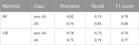
TABLE 1. Metrics related to the confusion matrix for the case in which all environmental covariates are considered for Random Forest (RF) and Gradient Boosting (GB). The two classes are non acid sulfate (non-AS) and acid sulfate (AS) soils.

TABLE 2

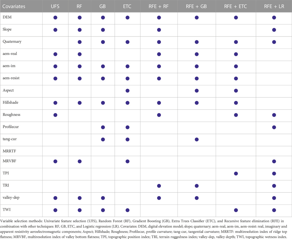
TABLE 2. Environmental covariates selected by different variable selection methods.

TABLE 3

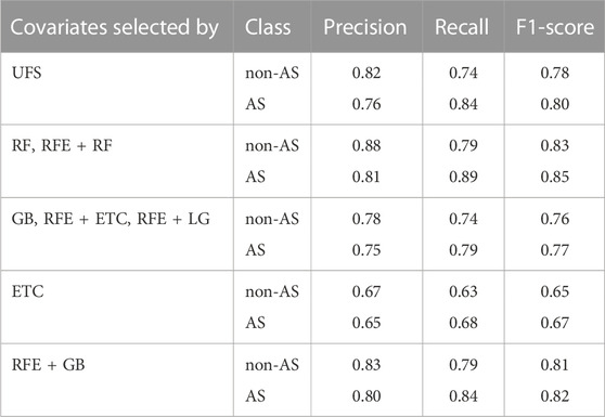
TABLE 3. Metrics related to the confusion matrix for different groups of environmental covariates for Random Forest (RF). The classes are acid sulfate (AS) and non acid sulfate (non-AS) soils.

TABLE 4

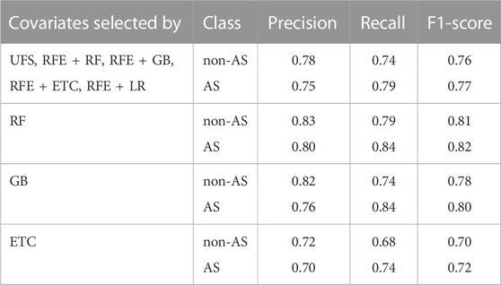
TABLE 4. Metrics related to the confusion matrix for different groups of environmental covariates for Gradient Boosting (GB). The classes are acid sulfate (AS) and non acid sulfate (non-AS) soils.

Another set of variables that gives very good results with RF is the one selected by RFE + RF (Table 3). However, for this group the results do not improve for GB with respect to the study of five covariates (Estévez et al., 2022). It should be noted that increasing the number of environmental covariates to ten improves the results of RF for all the groups except for the one selected by ETC (Table 3). On the contrary, in the case of GB, the increase of environmental covariates only improves the results for two cases, those selected by RF and GB (Table 4). Therefore, a greater number of variables generally benefits the classification in the case of RF but not necessarily when using GB. It could be related to the fact that unlike other methods, the consideration of irrelevant variables does not have a serious impact on the RF model (Kuhn and Johnson, 2013).

Contrary to the wrapped methods, the filter method UFS makes the selection based on the relationship between each environmental covariate and AS soils. Thus, the environmental covariates selected by this method give relevant information for the classification of AS soils. As it can be seen in Table 2, the covariates selected by UFS are the same as by RF except for one, roughness instead of quaternary. However, the results obtained for the group selected by UFS are not as good as for the one selected by RF, see Tables 3, 4. Even for the GB model the results for this group do not improve with respect to the previous study with five covariates (Estévez et al., 2022). This shows that the selection of each variable, as well as the combination between them, is extremely important for an accurate prediction or classification of AS soils.

So far, we have made the selection taking into account the importance of the covariates for the given methods. However, the redundancy of the variables is also very important for their selection. A pertinent question is how the correlation between variables affects the performance of the model. The linear correlation between the 17 environmental covariates considered in this study is shown in Figure 2. In the heatmap, dark green colors represent a strong positive correlation, whereas dark red colors indicate a strong negative correlation. A very low, low, moderate, high and very high correlation correspond to [0–0.2), [0.2–0.4), [0.4–0.6), [0.6–0.8) and [0.8–1], respectively. In general, variables with a high correlation provide redundant information, which can hinder the prediction. This could be the case of the group selected by RFE + LG, where some variables are strongly correlated with values close to one such as slope, roughness and TRI or profile curvature and TPI. For both, RF and GB models, the results obtained with this group are similar to the results by (Estévez et al., 2022) with five covariates and GB model. However, there are other covariates that are highly correlated and together give good results as in the case of the real and imaginary components of the aerogeophysics layers. Although these covariates are correlated, they also provide different information that can help to localize AS soils. The real component may show deep bedrock anomalies related to sulfide deposits, while the imaginary component allows the identification of weak surface anomalies associated to variations in the thickness of the topsoil. In order to analyze the role that the correlation is playing in the performance of the models, we have compared the correlation of two of the groups of variables. The two groups considered are those that have given the best and worst results. Curiously, the group with the best results, the one selected by RF, has more correlation than the one selected by ETC. Contrary to what might be expected, the group that shows the poorest results in the classification of AS soils has a very low correlation. Thus, a low correlation between the covariates does not guarantee the best prediction of the model. Comparing both groups, it can be seen that they only differ in three covariates, slope, real component of the aerogeophysics layer and valley depth in the group selected by RF, and aspect, profile curvature and tangential curvature in the ETC one (Table 2). Therefore, it seems that slope, real component of the aerogeophysics layer and valley depth are more important for the classification of AS soils than aspect, profile curvature or tangential curvature. Looking at Tables 2, 3 and Table 4, it is verified that the best results are obtained for the groups where these three covariates are presented. Moreover, valley depth is selected by 75% of the methods as one of the most important, slope and real component of the aerogeophysics layer by 62.5%, whereas aspect, profile curvature and tangential curvature are only selected by 37.5% of the methods. On the other hand, the correlation between the covariates selected by RFE + RF is very high. For example, slope, roughness, and TRI are strongly correlated with values close to one, and real and imaginary components of the aerogeophysics layer are highly correlated (Figure 2). In addition, there are several cases with moderate correlation. Despite the high correlation, the RF model also gives the best results for this group, but this is not the case for GB (Tables 3, 4). This could mean that GB is more affected by the correlation. By removing the slope and roughness of the RFE + RF group, the correlation related to the terrain layers disappears, and the results for both models improve. In the case of RF, the different metrics related to the confusion matrix increase between 1%–5%, leading to the best results of this model (Table 5). For GB, all the metrics improve by 5%, matching the best results obtained with this model for the group selected by RF (Table 4). Thus, for a good performance of the model there must be a balance between the importance of the covariates and their correlation.

FIGURE 2

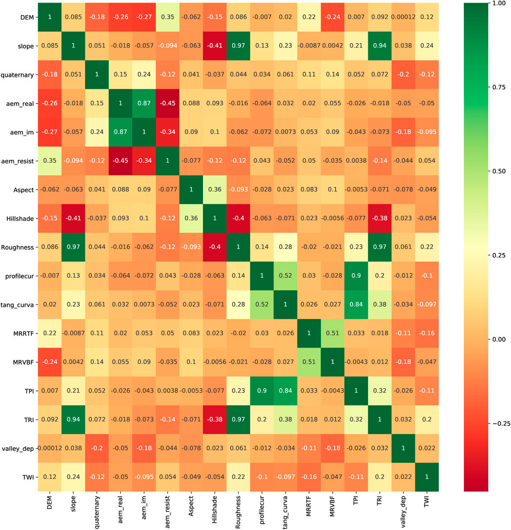
FIGURE 2. (Color online) Heatmap of Pearson correlation coefficient between the environmental covariates considered in the study.

TABLE 5

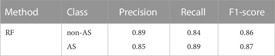
TABLE 5. Metrics related to the confusion matrix for the case RFE + RF without the correlation of the terrain layers and for the group selected by hand considering only the correlation for Random Forest (RF) model. The classes are acid sulfate (AS) and non acid sulfate (non-AS) soils.

In this work, the second way of variable selection has been carried out considering only the correlation. The selection has been made avoiding the high correlation between the covariates. If some variables have a correlation larger than 0.5 only one of them is selected. This allows to introduce more information in the model but without redundancy. All possible combinations have been analyzed, leading to different groups with eleven variables. It is worth highlighting the group formed by the following covariates: DEM, quaternary, imaginary and apparent resistivity components of the aerogeophysics layer, aspect, hillshade, tangential curvature, MRVBF, TRI, valley depth and TWI. For this group, RF also gives the best results, the same ones as for the case selected by RFE + RF but without slope and roughness (Table 5). For GB, the results for this group are similar to the results obtained with the group selected by RF except for the recall, which increases by 5% for AS soils but decreases by 5% for non-AS soils (Table 4). This once again demonstrates the complexity of variable selection.

The Backward Selection is the third method considered for variable selection in this study. As it was already explained in subsection 2.5.2.2, the method is based on the elimination of the irrelevant features for the model. Starting from the entire set of environmental covariates, the importance of each variable for the model is measured, and the most irrelevant one is removed. This process is repeated until the performance of the model stops improving. The importance of the variables is given by the model. In this study, Backward Selection has been analyzed using RF and GB. In the case of RF, the first covariate eliminated is MRRTF, which improves the results between 0%–5%. The second feature eliminated is the roughness, which leads to equal the results obtained by the groups selected by RF and RFE + RF (Table 3). However, removing the next least relevant covariate, MRVBF, the results are worse. For the GB model, the elimination of the first four irrelevant variables (MRVBF, TRI, MRRTF and slope) does not affect the results. By removing TPI, the results improve by 5%, matching the best results for this model, the ones obtained for the group selected by RF (Table 4). But by eliminating the following most irrelevant variable, aspect, the results are slightly worse. This indicates that the one-by-one backward selection method may select a set of variables that is not the best one for the performance of the model. This can be clearly seen in the case of the RF model, where the best results are obtained with 15 covariates. However, the same or better results are achieved with a smaller number of variables selected by other methods. The main problem with this backward selection is that the importance of the variables depends on the relationship between the variables considered, which changes as the variables are eliminated in each step. As already mentioned, an irrelevant variable by itself can be critical for a good performance of the model if other variables are present. Therefore, removing one of the variables can change the importance of certain variables. As a result, the selection of variables with this method is quite complex and does not guarantee that the variables selected are the most suitable for the model. It should be noted the difference between this one-by-one backward selection and the backward selection of the RFE method, where all variables are selected at the same time and are relevant to the model when they are together.

From all these results it can be seen that the environmental covariates DEM, slope, quaternary, the three components of the aerogephysics layers, hillshade, MRVBF, valley depth and TWI are very important for the classification of AS soils. In this study, the consideration of these covariates leads to a very accurate classification and prediction of this type of soil for the two models analyzed, RF and GB. In general, for the same groups of covariates better results are obtained with RF than with GB. It should be noted that the RF model improves the accuracies between 15%–17% for the case of eight relevant covariates with respect to a previous study where five covariates were considered (Estévez et al., 2022). Unlike RF, the results for most of the groups analyzed with the GB model do not improve with the increase of the number of covariates. Furthermore, in the cases in which the results improve with respect to the case of five covariates, the accuracies improve by at most 5%. In the study by (Estévez et al., 2022), the accuracies obtained with the GB model are 5%–6% higher than those obtained with the RF model. This leads to two pertinent questions: Is GB a model that works better for a small number of covariates? or are these results related to the importance of the covariates considered? In order to answer these questions, a new group of five covariates has been analyzed. In the case of RF, there are six covariates that appear in all the groups with the best results, i.e., with values of F1-score equal or larger than 0.83 and 0.85 for non-AS and AS soils, respectively (Tables 3, 5). These environmental covariates are: DEM, quaternary, imaginary and apparent resistivity components of the aerogeophysics layer, hillshade and valley depth. As the quaternary layer is very relevant for GB, this layer is not included in the study. For this set of variables, the RF model improves the classification between 5%–6% with respect to the results obtained in a previous work where the five covariates considered were DEM, slope, quaternary, real and imaginary components of the aerogeophysics layer (Estévez et al., 2022). For GB, the results obtained for this set of variables are worse than the ones for the previous work. This is because the quaternary layer, which is very important for GB model, is not included in this study. Thus, this shows the great importance of the selection of features in the classification and prediction of AS soils for each model.

3.2 Probability map for acid sulfate soil occurrences

In general the accuracies obtained in this study are greater for RF than for GB. Therefore, RF is the model chosen for the mapping of AS soils. The group of covariates from which the best results have been obtained is the one used to create the AS soil probability map. There are two sets of variables that have given the best results with the RF model (Table 5), one where only the correlation was taken into account in the selection, and the other the one selected by RFE + RF without the correlation between terrain layers. The first one has eleven covariates whereas the second one eight covariates. In general, smaller datasets reduce computation time (Guyon and Elisseeff, 2003). Although in our case there will be hardly any difference between the two groups, the smaller one has been used. Figure 3 shows the AS soil probability map created with RF for the group composed of the environmental covariates: DEM, quaternary, the real, imaginary and apparent resistivity components of the aerogephysics layer, hillshade, TRI and valley depth. The prediction of the probability of encountering AS soils has been performed for each of the 434,036 cells of 50 m × 50 m that make up the study area. The calculation is based on the values of the environmental covariates. For the representation of the map, the probability of encountering AS soils has been divided into four different probability classes: very low, low, high and very high, which correspond to [0–0.25), [0.25–0.5), [0.5–0.75) and [0.75–1], respectively. The corresponding areas of the AS soil probability map in percentage and km² for each probability class are represented in Table 6. For 21% of the study area the probability of encountering AS soils is high and very high, whereas in the remaining 79% the probability is low and very low. As has already been mentioned, the RF model for this group of covariates increases the accuracies with respect to the previous study (Estévez et al., 2022), between 15%–17% for the RF model and between 10%–11% for the GB model. Comparing the AS soil probability maps created with the RF model in both cases, it can be seen that the areas with very high, high and very low probabilities are smaller in the present map, the one with greater accuracies. On the contrary, the area with low probability has increased to represent about half (51%) of the study area (Table 6). It should be noted that approximately 58% of the uppermost meter in the study area is made up of bedrock, outcrops and block fields, where the probability of encountering AS soils is usually very low to low. Although the model has not been trained with samples from the areas where bedrock, outcrops and rockfields are located, the model has predicted around 86% of these areas as very low and low probability. This demonstrates a high ability of the RF model to predict and classify AS soils with this set of environmental covariates.

FIGURE 3

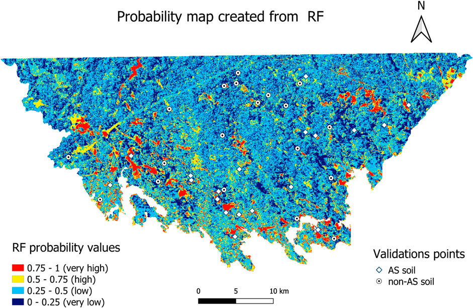
FIGURE 3. (Color online) Probability map created from Random Forest (RF) for the covariate group selected by RFE + RF without slope and roughness.

TABLE 6

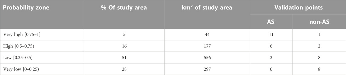
TABLE 6. Validation of the probability map created from Random Forest (RF) for the group of covariates: DEM, quaternary, aem-real, aem-im, aem-resist, hillshade, TRI and valley depth. Validation points are acid sulfate (AS) and non-acid sulfate (non-AS) soils.

On the other hand, there is a linear feature in the probability map (Figure 3), which is related to a visible power line in the aerogeophysics layers. These layers show the components of the electromagnetic induction, which is very strong in the power line. Thus, the information of the area of the line is related to the power line but not to the soil. This can affect the prediction of the model for the area of the power line depending on the importance of the different covariates. If the aerogeophysics layers are very important for the model, the prediction in the area of the power line may be incorrect. A more accurate prediction will be made if some of the covariates that give soil information in the power line area are the most relevant for the model. Unlike the line feature shown in the AS soil probability maps created with different models in the previous study (Estévez et al., 2022), the line feature is not as sharp on this map, i.e., the predictions for this line are much more similar to the predictions of the neighboring cells (Figure 3). This is due to the number of covariates that give information about the soil in the area of the power line is larger in this study, which facilitates a more accurate prediction. In order to avoid possible linear features in the maps in future studies, it should be good to mask any power lines present in the aerogeophysics layers before doing the prediction for the area.

Finally, the validation of the AS soil probability map can be performed by comparing the validation points to the prediction made by the model for the cells where these points are located. These results are shown in Table 6. For this validation, the same points used to evaluate the models for the different groups of environmental covariates have been considered. These validation points are displayed in the probability map (Figure 3). For the AS soil validation points, 89% of the predicted probability classes for the corresponding cells are correctly classified. Most of these points (65%) are located in areas predicted as very high probability areas, whereas the remaining points (35%) in high probability areas. There are two points located in cells that have been predicted as belonging to the low probability class. For the case of non-AS soils validation points, 84% of their corresponding cells are correctly classified in the low and very low probability areas in equal proportion for both areas (Table 6). There are three validation points (16%) located in cells that have been incorrectly classified, two points are in the high probability area and one point in the very high probability area.

3.3 Extents of acid sulfate soil areas

The main objective of mapping the occurrence of the AS soils is to locate areas that could have a negative environmental impact if the soil materials are disturbed for instance in agriculture and during infrastructure developments. Furthermore, it is important to know the extent of AS soils in order to estimate potential or ongoing mobilization of environmentally hazardous elements (e.g., Cd and Ni) into watercourses. So far, the extent of AS soils has been calculated from conventional occurrence maps. In the study area, a conventional probability map of AS soil occurrence within the Littorina Sea maximum extent area (83% of the study area) was presented in (Estévez et al., 2022). This conventional AS soil probability map has four different probability classes: high, moderate, low and very low, which probabilities of encountering AS soils are 98.5%, 52.5%, 1.7% and 0%, respectively. The total area of the conventional map is 904.48 km², where 24.65 km² corresponds to the high class, 78.88 km² to the moderate class, 207.72 km² to the low class and 593.23 km² to the very low class. In this paper, the extent of AS soils for this conventional map has been calculated based on a similar approach previously used for calculating the extent of AS soils in Denmark (Madsen and Jensen, 1988). In total, the study area comprises 69.29 km² AS soils (7.7% of the area) of which 24.28 km² are present in the high probability class, 41.43 km² in the moderate probability class and 3.58 km² in the low probability class. The distribution of roughly 8% of AS soils in the study area is considerably somewhat lower compared to a larger area of 3,106 km² located in Northern Ostrobothnia, Finland, where about 25% of the total area is covered by AS soils (Becher et al., 2019). This discrepancy is most likely due to differences in topography between the two regions, with much more variation in the study area and with a general abundance of bedrock outcrops and a lack of larger rivers feeding sedimentary basins with sediment and organic matter required for iron sulfide formation in southern Finland. However, it should be noted that almost 60% of the study area described in this paper is covered by bedrock, outcrops and block fields that could not be sampled. In the conventional AS soil occurrence map, the probability of finding AS soils in an area is determined from the proportion of soil samples classified as AS soils and the total number of soil samples of the area. Thus, the probability of the 60% of the study area is equal to zero as there are not soil samples in that area. This may affect the estimation of the extent of AS soils in the conventional AS soil probability map.

In this paper, a new approach for the calculation of the extent of AS soils in modeled AS soil probability maps is shown. Unlike in the conventional map, the probability of encountering AS soils in a modeled probability map has been calculated for each pixel of the map (50 m × 50 m). Therefore, the extent of AS soils can be calculated by multiplying each pixel area by its probability of finding AS soils. This allows a much more accurate calculation of the extent of AS soils. The extent of AS soils in the modeled probability map has been calculated for the same area as the conventional map, the part corresponding to the Littorina Sea maximum extent. The total extent of AS soils in the modeled map is 315.5 km², of which 42.7 km² are located in the very high probability area, 87.2 km² in the high probability area, 151.5 km² in the low probability area and 34.1 km² in the very low probability area. The total extent of AS soils represents 35% of the study area. This value must be interpreted as the maximum extent of AS soils as all cells of the map have been considered. For the potential environmental hazards, it should be noted that only 129.9 km² of the calculated extents of AS soils have a probability of encountering AS soils greater than 50%.

4 Conclusion

As it has been shown in this study, considering a larger number of environmental covariates does not necessarily improve the prediction of the model. For this reason, in this study, variable selection has been used to improve the prediction accuracy for acid sulfate soil mapping. Eleven different variable selection methods have been considered for the selection of the most relevant environmental covariates for the correct classification and prediction of acid sulfate (AS) soils. Among the most frequently chosen variables are those selected by Random Forest (RF). Furthermore, the best results for the two modeling methods, RF and Gradient Boosting (GB), have been obtained for the group of covariates selected by RF. Therefore, in this case study, RF is a very good method in the selection of environmental covariates for the prediction of AS soils. On the contrary, Extra Trees Classifier (ETC) is the method whose selection of environmental covariates has led to the worst results for both modeling methods.

On the other hand, it has been seen that the combination of two variable selection methods can improve the prediction accuracy. This has been the case when considering RFE + RF and Pearson’s correlation, where the results have improved between 1%–5%, if the correlation is taken into account. However, it has been seen that the correlation alone is not enough to select the most important covariates for the prediction of AS soils. For instance, there are strongly correlated covariates such as the real and imaginary components of the aerogeophysical layers that combined have given very good results in the prediction. Others covariates, such as highly correlated terrain layers, have made prediction difficult. Furthermore, it has been shown that a group of covariates without correlation does not necessarily give a good prediction. Finally, the results of the Backward Selection analysis have shown that this method does not generally select the most appropriate covariates for a correct model prediction.

In general, better results have been obtained in the prediction of AS soils with the RF model than with the GB model. The AS soil probability map has been created for the group of covariates with the best results in prediction for the RF model. Variable selection has enabled the RF model to improve the results of the prediction by up to 15%–17% for a group of eight covariates as compared with a previous study in the same area where five covariates were considered. It should be noted that this improvement is not produced by the increase of three extra covariates in the study, but by the consideration of eight covariates in particular. For eight different layers, that improvement does not occur. This demonstrates the importance of variable selection for the prediction of AS soils. From the validation of the AS soil probability map, it can be seen that the model has been able to correctly predict 89% of the cells where the validation points are located for AS soils, and 84% for non-AS soils. Finally, this study presents a new approach that allows an accurate estimation of the extent of AS soils in modeled probability maps.

Future studies should address the importance of these selected environmental covariates for classification and prediction of AS soils in other areas where AS soils may be slightly different. Another important study would be the analysis of the relevance of these environmental covariates for machine learning methods with a very different algorithm, such as a Convolutional Neural Network.

Data availability statement

The raw data supporting the conclusion of this article will be made available by the authors, without undue reservation.

Author contributions

VE carried out the research, performed the analysis and modeling, and wrote the paper. SM and ABo contributed to write the paper. All authors contributed to the article and approved the submitted version.

Funding

This work has been financially supported by Stiftelsen Arcada foundation (Finland).

Conflict of interest

The authors declare that the research was conducted in the absence of any commercial or financial relationships that could be construed as a potential conflict of interest.

Publisher’s note

All claims expressed in this article are solely those of the authors and do not necessarily represent those of their affiliated organizations, or those of the publisher, the editors and the reviewers. Any product that may be evaluated in this article, or claim that may be made by its manufacturer, is not guaranteed or endorsed by the publisher.

References

Airo, M-L. (2005). Aerogephysics in Finland 1972-2004 methods, system characteristics and applications. Geol. Surv. Finl., 197. Special Paper 39. Espoo, Finland.

Google Scholar

Airo, M.-L., and Loukola-Ruskeeniemi, K. (2004). Characterization of sulfide deposits by airborne magnetic and gamma-ray responses in eastern Finland. Ore Geol. Rev. 24, 67–84. doi:10.1016/j.oregeorev.2003.08.008

CrossRef Full Text | Google Scholar

Akusok, A., Björk, K. M., Estévez, V., and Boman, A. (2023). “Randomized model structure selection approach for Extreme learning machine applied to acid sulfate soil detection,” in Proceedings of ELM 2021. ELM 2021. Proceedings in adaptation, learning and optimization. Editor K. M. Björk (Cham: Springer). doi:10.1007/978-3-031-21678-7_4

CrossRef Full Text | Google Scholar

Åström, M., and Björklund, A. (1997). Geochemistry and acidity of sulphide-bearing postglacial sediments of Western Finland. Environ. Geochem. Health 19, 155–164. doi:10.1023/a:1018462824486

CrossRef Full Text | Google Scholar

Azizi, K., Ayoubi, S., Nabiollahi, K., Garosi, Y., and Gislum, R. (2022). Predicting heavy metal contents by applying machine learning approaches and environmental covariates in west of Iran. J. Geochem. Explor. 233, 106921. doi:10.1016/j.gexplo.2021.106921

CrossRef Full Text | Google Scholar

Becher, M., Sohlenius, G., Öhrling, C., Boman, A., Josefsson, S., Mattbäck, S., et al. (2019). “Acid sulphate soils around coastal watercourses, Project report,” in 2019, coastal watercourses - methodological development and restoration. Final report, 189. Interreg Nord 2014-2020.

Google Scholar

Becher, M., Sohlenius, G., Öhrling, C., Boman, A., Josefsson, S., and Mattbäck, S. (2018). Sur sulfatjord runt kustmynnande vattendrag. Technical report. Uppsala, Sweden: Geological Survey of Sweden and Geological Survey of Finland, 35.

Google Scholar

Behrens, T., Schmidt, K., Zhu, A. X., and Scholten, T. (2010). The ConMap approach for terrain-based digital soil mapping. Eur. J. Soil Sci. 61, 133–143. doi:10.1111/j.1365-2389.2009.01205.x

CrossRef Full Text | Google Scholar

Beucher, A., Rasmussen, C. B., Moeslund, T. B., and Greve, M. H. (2022). Interpretation of convolutional neural networks for acid sulfate soil classification. Front. Environ. Sci. 9, 809995. doi:10.3389/fenvs.2021.809995

CrossRef Full Text | Google Scholar

Beucher, A., Adhikari, K., Breuning-Madsen, H., Greve, M. B., Österholm, P., Fröjdö, S., et al. (2017). Mapping potential acid sulfate soils in Denmark using legacy data and LiDAR-based derivatives. Geoderma 308, 363–372. doi:10.1016/j.geoderma.2016.06.001

CrossRef Full Text | Google Scholar

Beucher, A., Fröjö, S., Österholm, P., Martinkauppi, A., and Edén, P. (2014). Fuzzy logic for acid sulfate soil mapping: Application to the southern part of the Finnish coastal areas. Geoderma 226-227, 21–30. doi:10.1016/j.geoderma.2014.03.004

CrossRef Full Text | Google Scholar

Beucher, A., Österholm, P., Martinkauppi, A., Edén, P., and Fröjö, S. (2013). Artificial neural network for acid sulfate soil mapping: Application to the Sirppujoki River catchment area, south-Western Finland. J. Geochem Explor 125, 46–55. doi:10.1016/j.gexplo.2012.11.002

CrossRef Full Text | Google Scholar

Beucher, A., Siemssen, R., Fröjö, S., Österholm, P., Martinkauppi, A., and Edén, P. (2015). Artificial neural network for mapping and characterization of acid sulfate soils: Application to Sirppujoki River catchment, southwestern Finland. Geoderma 247-248, 38–50. doi:10.1016/j.geoderma.2014.11.031

CrossRef Full Text | Google Scholar

Boman, A., Becher, M., Mattbäck, S., Sohlenius, G., Auri, J., Öhrling, C., et al. (2019). Classification of acid sulphate soils in Finland and Sweden. Appendix 1, p. In, Coastal watercourses - methodological development and restoration. Final report, Interreg Nord 2014-2020, 189 p. Available at: https://www.lansstyrelsen.se/norrbotten/tjanster/publikationer/coastal-watercourses—methodological-development-and-restoration.html

Google Scholar

Breiman, L. (2001). Random forests. Mach. Learn. 45, 5–32. doi:10.1023/a:1010933404324

CrossRef Full Text | Google Scholar

Brungard, C. W., Boettinger, J. L., Duniway, M. C., Wills, S. A., and Edwards, T. C. (2015). Machine learning for predicting soil classes in three semi-arid landscapes. Geoderma 239-240, 68–83. doi:10.1016/j.geoderma.2014.09.019

CrossRef Full Text | Google Scholar

Brus, D. J., Kempen, B., and Heuvelink, G. B. M. (2011). Sampling for validation of digital soil maps. Eur. J. Soil Sci. 62, 394–407. doi:10.1111/j.1365-2389.2011.01364.x

CrossRef Full Text | Google Scholar

Camera, C., Zomeni, Z., Noller, J. S., Zissimos, A. M., Christoforou, I. C., and Bruggeman, A. (2017). A high resolution map of soil types and physical properties for Cyprus: A digital soil mapping optimization. Geoderma 285, 35–49. doi:10.1016/j.geoderma.2016.09.019

CrossRef Full Text | Google Scholar

Campling, P., Gobin, A., and Feyen, J. (2002). Logistic modeling to spatially predict the probability of soil drainage classes. Soil Sci. Soc. Am. J. 66, 1390–1401. doi:10.2136/sssaj2002.1390

CrossRef Full Text | Google Scholar

Campos, A. R., Giasson, E., Costa, J. J. F., Machado, I. R., Silva, E. B., and Bonfatti, B. R. (2018). Selection of environmental covariates for classifier training applied in digital soil mapping. Rev. Bras. Cienc. Solo. 42, e0170414. doi:10.1590/18069657rbcs20170414

CrossRef Full Text | Google Scholar

Castro Franco, M., Domenech, M., Costa, J. L., and Aparicio, V. C. (2017). Modelling effective soil depth at field scale from soil sensors and geomorphometric indices. Acta Agronómica. 66 (2), 227–234. doi:10.15446/acag.v66n2.53282

CrossRef Full Text | Google Scholar

Chen, Y., Ma, L., Yu, D., Zhang, H., Feng, K., Wang, X., et al. (2022). Comparison of feature selection methods for mapping soil organic matter in subtropical restored forests. Ecol. Indic. 135, 108545. doi:10.1016/j.ecolind.2022.108545

CrossRef Full Text | Google Scholar

Debella-Gilo, M., and Etzelmüller, B. (2009). Spatial prediction of soil classes using digital terrain analysis and multinomial logistic regression modeling integrated in GIS: Examples from Vestfold County, Norway. Catena 77, 8–18. doi:10.1016/j.catena.2008.12.001

CrossRef Full Text | Google Scholar

Estévez Nuño, V. (2020). Machine learning methods for classification of acid sulfate soils in Virolahti. Master’s thesis. Finland: Arcada University of Applied Sciences. Jan-Magnus Janssons plats 1, 00560 Helsinki, Finland (June 2020).

Google Scholar

Estévez, V., Beucher, A., Mattbäck, S., Boman, A., Björk, K-M., Osterhölm, P., et al. (2022). Machine learning techniques for acid sulfate soil mapping in southeastern Finland. Geoderma 406, 115446. doi:10.1016/j.geoderma.2021.115446

CrossRef Full Text | Google Scholar

Estévez, V., Mattbäck, S., and Björk, K-M. (2023). Importance of the activation function in Extreme Learning Machine for Acid sulfate soil classification. Presented at ELM 2022 – Dec 8-9, 2022, Virtual Conference (Main location Helsinki – Finland).

Fitzpatrick, B. R., Lamb, D. W., and Mengersen, K. (2016). Ultrahigh dimensional variable selection for interpolation of point referenced spatial data: A digital soil mapping case study. PLoS ONE 11 (9), e0162489. doi:10.1371/journal.pone.0162489

PubMed Abstract | CrossRef Full Text | Google Scholar

Forman, G. (2003). An extensive empirical study of feature selection metrics for text classification. J. Mach. Learn. Res. 3, 1289–1305. doi:10.1162/153244303322753670

CrossRef Full Text | Google Scholar

Friedman, J. H. (2001). Greedy function approximation: A gradient boosting machine. Ann. Stat. 29 (5), 1189–1232. doi:10.1214/aos/1013203451

CrossRef Full Text | Google Scholar

Gambill, D. R., Wall, W. A., Fulton, A. J., and Howard, H. R. (2016). Predicting USCS soil classification from soil property variables using Random Forest. J. Terramechanics 65, 85–92. doi:10.1016/j.jterra.2016.03.006

CrossRef Full Text | Google Scholar

Geological Survey of Finland (2021). Acid sulfate soils – map services. Finland: Geological Survey of Finland. http://gtkdata.gtk.fi/hasu/index.html.

Google Scholar

Geurts, P., Ernst, D., and Wehenkel, L. (2006). Extremely randomized trees. Mach. Learn. 1, 3–42. doi:10.1007/s10994-006-6226-1

CrossRef Full Text | Google Scholar

Giasson, E., Clarke, R. T., Vasconcellos Inda Junior, A., Merten, G. H., and Tornquist, C. G. (2006). Digital soil mapping using multiple logistic regression on terrain parameters in southern Brazil. Sci. Agric. (Piracicaba, Braz.) 63 (3), 262–268. doi:10.1590/s0103-90162006000300008

CrossRef Full Text | Google Scholar

Grimm, R., Behrens, T., Maerker, M., and Elsenbeer, A. (2008). Soil organic carbon concentrations and stocks on Barro Colorado Island — digital soil mapping using Random Forests analysis. Geoderma 146, 102–113. doi:10.1016/j.geoderma.2008.05.008

CrossRef Full Text | Google Scholar

Guyon, I., and Elisseeff, A. (2003). An introduction to variable and feature selection. J. Mach. Learn. Res. 3, 1157–1182. doi:10.1162/153244303322753616

CrossRef Full Text | Google Scholar

Guyon, I., Weston, J., Barnhill, S., and Vapnik, V. (2002). Gene selection for cancer classification using Support vector machines. Mach. Learn. 46, 389–422. doi:10.1023/a:1012487302797

CrossRef Full Text | Google Scholar

Haavisto-Hyvärinen, M., and Kutvonen, H. (2007). Maaperäkartan käyttöopas. Finland: Geological Survey of Finland.

Google Scholar

Hall, M. A., and Holmes, G. (2003). Benchmarking attribute selection techniques for discrete class data mining. IEEE Trans. Knowl. Data Eng. 15 (6), 1437–1447. doi:10.1109/TKDE.2003.1245283

CrossRef Full Text | Google Scholar

Hengl, T., Mendes de Jesus, J., Heuvelink, G. B. M., Ruiperez Gonzalez, M., Kilibarda, M., Blagotić, A., et al. (2017). SoilGrids250m: Global gridded soil information based on machine learning. PLoS One 12, e0169748. doi:10.1371/journal.pone.0169748

PubMed Abstract | CrossRef Full Text | Google Scholar

Heung, B., Bulmer, C. E., and Schimdt, M. G. (2014). Predictive soil parent material mapping at a regional-scale: A random forest approach. Geoderma 214-215, 141–154. doi:10.1016/j.geoderma.2013.09.016

CrossRef Full Text | Google Scholar

Heung, B., Ho, H. C., Zhang, J., Knudby, A., Bulmer, C. E., and Schimdt, M. G. (2016). An overview and comparison of machine-learning techniques for classification purposes in digital soil mapping. Geoderma 265, 62–77. doi:10.1016/j.geoderma.2015.11.014

CrossRef Full Text | Google Scholar

Huang, J., Nhan, T., Wong, V. N. L., Johnston, S. G., Lark, R. M., and Triantafilis, J. (2014). Digital soil mapping of a coastal acid sulfate soil landscape. Soil Res. 52, 327–339. doi:10.1071/sr13314

CrossRef Full Text | Google Scholar

Hudd, R. (2000). Springtime episodic acidification as a regulatory factor of estuary spawing fish recruitment. PhD Thesis. Finland: Helsinki University.

Google Scholar

Jafari, A., Finkeb, P. A., Van de Wauwb, J., Ayoubi, S., and Khademi, H. (2012). Spatial prediction of USDA-great soil groups in the arid zarand region, Iran: Comparing logistic regression approaches to predict diagnostic horizons and soil types. Eur. J. Soil Sci. 63, 284–298. doi:10.1111/j.1365-2389.2012.01425.x

CrossRef Full Text | Google Scholar

Keskin, H., Grunwald, S., and Harris, W. G. (2019). Digital mapping of soil carbon fractions with machine learning. Geoderma 339, 40–58. doi:10.1016/j.geoderma.2018.12.037

CrossRef Full Text | Google Scholar

Kohavi, R., and John, G. H. (1997). Wrappers for features subset selection. Artif. Intell. 97, 1–2.

CrossRef Full Text | Google Scholar

Korpela, K., and Niemelä, O. (1985). Maaperäkartat 1:20 000 ja 1:50 000. Maankäyttö 2.

Kuhn, M., and Johnson, K. (2013). Applied predictive modeling. New York: Springer.

Google Scholar

Lacoste, M., Mulder, V. L., Richer-de-Forges, A. C., Martin, M. P., and Arrouays, D. (2016). Evaluating large-extent spatial modeling approaches: A case study for soil depth for France. Geoderma Reg. 7, 137–152. doi:10.1016/j.geodrs.2016.02.006

CrossRef Full Text | Google Scholar

Lehtinen, M., Nurmi, P., and Rämö, T. (1998). Suomen kallioperä: 3000 vuosimiljoonaa. Helsinki: Suomen Geologinen Seura ry., 375.

Google Scholar

Lemercier, B., Lacoste, M., Loum, M., and Walter, C. (2012). Extrapolation at regional scale of local soil knowledge using boosted classification trees: A two-step approach. Geoderma 171-172, 75–84. doi:10.1016/j.geoderma.2011.03.010

CrossRef Full Text | Google Scholar

Li, X., Luo, J., Jin, J., He, Q., and Niu, Y. (2020). Improving soil thickness estimations based on multiple environmental variables with stacking ensemble methods. Remote Sens. 12, 3609. doi:10.3390/rs12213609

CrossRef Full Text | Google Scholar

Lie, M., Glaser, B., and Huwe, B. (2012). Uncertainty in the spatial prediction of soil texture: Comparison of regression tree and Random Forest models. Geoderma 15, 70. doi:10.1016/j.geoderma.2011.10.010

CrossRef Full Text | Google Scholar

Lie, M., Schmidt, J., and Glaser, B. (2016). Improving the spatial prediction of soil organic carbon stocks in a complex tropical mountain landscape by methodological specifications in machine learning approaches. PLoS ONE 11 (4), e0153673. doi:10.1371/journal.pone.0153673

PubMed Abstract | CrossRef Full Text | Google Scholar

Lu, Y.-Y., Liu, F., Zhao, Y.-G., Song, X.-D., and Zhang, G-L. (2019). An integrated method of selecting environmental covariates for predictive soil depth mapping. J. Integr. Agric. 18 (2), 301–315. doi:10.1016/s2095-3119(18)61936-7

CrossRef Full Text | Google Scholar

Madsen, H. B., and Jensen, N. H. (1988). Potentially acid sulfate soils in relation to landforms and geology. Catena 15, 137–145. doi:10.1016/0341-8162(88)90025-2

CrossRef Full Text | Google Scholar

Mattbäck, S., Boman, A., and Österholm, P. (2017). Hydrogeochemical impact of coarse-grained post-glacial acid sulfate soil materials. Geoderma 308, 291–301. doi:10.1016/j.geoderma.2017.05.036

CrossRef Full Text | Google Scholar

McBratney, A., Mendonça Santos, M. L., and Minasny, B. (2003). On digital soil mapping. Geoderma 117, 3–52. doi:10.1016/s0016-7061(03)00223-4

CrossRef Full Text | Google Scholar

Michael, P. S. (2013). Ecological impacts and management of acid sulphate soil: A review. Asian J. Water, Environ. Pollut. 10 (No. 4), 13–24.

Google Scholar

Moradpour, S., Entezari, M., Ayoubi, S., Karimi, A., and Naimi, S. (2023). Digital exploration of selected heavy metals using Random Forest and a set of environmental covariates at the watershed scale. J. Hazard. Mater. 455, 131609. doi:10.1016/j.jhazmat.2023.131609

PubMed Abstract | CrossRef Full Text | Google Scholar

Müller, A. C., and Guido, S. (2016). An introduction to machine learning with Python. Sebastopol, CA 95472: O’Reilly Media, Inc., 1005 Gravenstein Highway North.

Google Scholar

Osl, M., Dreiseitl, S., Cerqueira, F., Netzer, M., Pfeifer, B., et al. (2009). Demoting redundant features to improve the discriminatory ability in cancer data. J. Biomed. Inf. 42, 721–725. doi:10.1016/j.jbi.2009.05.006

CrossRef Full Text | Google Scholar

Österholm, P., and Åström, M. (2002). Spatial trends and losses of major and trace elements in agricultural acid sulphate soils distributed in the artificially drained Rintala area, W. Finland. W. Finl. Appl. Geochem. Vol. 17 (9), 1209–1218. doi:10.1016/s0883-2927(01)00133-0

CrossRef Full Text | Google Scholar

Österholm, P., Åström, M., and Sundström, R. (2005). Assessment of aquatic pollution, remedial measures and juridical obligations of an acid sulphate soil area in Western Finland. Agric. Food Sci. 14, 44–56. doi:10.2137/1459606054224101

CrossRef Full Text | Google Scholar

Palko, J. (1994). Acid sulphate soils and their agricultural and environmental problems in Finland. Finland: Acta University Oulu, C75. University Oulu.

Google Scholar

Pedregosa, F., Varoquaux, G., Gramfort, A., Michel, V., Thirion, B., Grisel, O., et al. (2011). Scikit-learn: Machine learning in Python. J. Mach. Learn. Res. 12, 2825–2830.

Google Scholar

Pernu, T. (1991). Model and field studies of direct current resistivity measurements with the combined (half-Schlumberger) array Amn. MNB Acta Univ. Ouluensis, Ser. A, Sci. Rerum Nat. 221, 123.

Google Scholar

Pons, L. J. (1973). “Outline of the Genesis,characteristics, classification and improvement of acid sulfate soils,” in Acid sulphate soils, Introductory papers and bibliography, ILRI Publication 18. Proceedings of the international symposium 13-20. Editor H. Dost (Wageningen), 3–27.

Google Scholar

Porwal, A., Carranza, E. J. M., and Hale, M. (2003). Artificial neural networks for mineral potential mapping: A case study from aravalli province, western India. Nat. Resour. Res. 12 (3), 155–171. doi:10.1023/a:1025171803637

CrossRef Full Text | Google Scholar

Powers, D. M. W. (2011). Evaluation: From precision, recall, and F-measure to ROC, informedness, markedness & correlation. J. Mach. Learn. Technol. V 2, 37–63.

Google Scholar

QGIS Development Team (2019). QGIS geographic information system. Open Source Geospatial Foundation Project http://qgis.osgeo.org.

Google Scholar

Roos, M., and Åström, M. (2006). Gulf of Bothnia receives high concentrations of potentially toxic metals from acid sulphate soils. Boreal Environ. Res. 11, 383–388.

Google Scholar

Saeys, Y., Inza, I., and Larrañaga, P. (2007). A review of feature selection techniques in bioinformatics. Bioinformatics 23 (Issue 19), 2507–2517. doi:10.1093/bioinformatics/btm344

PubMed Abstract | CrossRef Full Text | Google Scholar

Schmidt, K., Behrens, T., Daumann, J., Ramirez-Lopez, L., Werban, U., Dietrich, P., et al. (2014). A comparison of calibration sampling schemes at the field scale. Geoderma 232–234, 243–256. doi:10.1016/j.geoderma.2014.05.013

PubMed Abstract | CrossRef Full Text | Google Scholar

Sindayiheburaa, A., Ottoyb, S., Dondeyneb, S., Van Meirvennec, M., and Van Orshovenb, J. (2017). Comparing digital soil mapping techniques for organic carbon and clay content: Case study in Burundi’s central plateaus. Catena 156, 161–175. doi:10.1016/j.catena.2017.04.003

CrossRef Full Text | Google Scholar

Teng, H. T., Viscarra Rossel, R. A., Shi, Z., and Behrens, T. (2018). Updating a national soil classification with spectroscopic predictions and digital soil mapping. Catena 164, 125–134. doi:10.1016/j.catena.2018.01.015

CrossRef Full Text | Google Scholar

Tesfa, T. K., Tarboton, D. G., Chandler, D. G., and McNamara, J. P. (2009). Modeling soil depth from topographic and land cover attributes. Water Resour. Res. 45, 1–16. doi:10.1029/2008wr007474

CrossRef Full Text | Google Scholar

Tziachrisa, P., Aschonitisa, V., Chatzistathisa, T., and Papadopoulou, M. (2019). Assessment of spatial hybrid methods for predicting soil organic matter using DEM derivatives and soil parameters. Catena 174, 206–216. doi:10.1016/j.catena.2018.11.010

CrossRef Full Text | Google Scholar

Urho, L. (2002). The importance of larvae and nursery areas for fish production. Finland: Helsinki University, 135.

Google Scholar

Van Rossum, G., and Drake, F. L. (2009). Python 3 reference manual, scotts valley. CA: CreateSpace.

Google Scholar

Veronesi, F., and Schillaci, C. (2019). Comparison between geostatistical and machine learning models as predictors of topsoil organic carbon with a focus on local uncertainty estimation. Ecol. Indic. V. 101, 1032–1044. doi:10.1016/j.ecolind.2019.02.026

CrossRef Full Text | Google Scholar

Wei, Q., and Dunbrack, R. L. (2013). The role of balanced training and testing data sets for binary classifiers in bioinformatics. PLOS ONE 8 (7), e67863. doi:10.1371/journal.pone.0067863

PubMed Abstract | CrossRef Full Text | Google Scholar

Weiss, G., and Provost, F. (2001). The effect of class distribution on classifier learning: An empirical study. Tech. Rep.

Google Scholar

Wiesmeier, M., Barthold, F., Blank, B., and Kögel-Knabner, I. (2011). Digital mapping of soil organic matter stocks using Random Forest modeling in a semi-arid steppe ecosystem. Plant Soil 340, 7–24. doi:10.1007/s11104-010-0425-z

CrossRef Full Text | Google Scholar

Xiong, X., Grunwald, S., Myers, D. B., Kim, J., Harris, W. G., and Comerford, N. B. (2014). Holistic environmental soil-landscape modeling of soil organic carbon./ Environ. Model. Softw. 57, 202–215. doi:10.1016/j.envsoft.2014.03.004

CrossRef Full Text | Google Scholar

Yli-Halla, M., and Mokma, D. L. (1998). Soil temperature regimes in Finland. Agric. food Sci. Finl. 7, 507–512. doi:10.23986/afsci.5606

CrossRef Full Text | Google Scholar

Yli-Halla, M., Puustinen, M., and Koskiaho, J. (1999). Area of cultivated acid sulfate soils in Finland. Soil Use Manag. 15, 62–67. doi:10.1111/j.1475-2743.1999.tb00065.x

CrossRef Full Text | Google Scholar