 Kaltham A. Ismail
 Maryam R. Al-Shehhi
- Department of Civil, Infrastructure and Environmental Engineering, Khalifa University, Abu Dhabi, United Arab Emirates
Marine biogeochemical models are an effective tool for formulating hypothesis and gaining mechanistic understanding of how an ecosystem functions. This paper presents a comprehensive review of biogeochemical models and explores their applications in different marine ecosystems. It also assesses their performance in reproducing key biogeochemical components, such as chlorophyll-a, nutrients, carbon, and oxygen cycles. The study focuses on four distinct zones: tropical, temperate, polar/subpolar, and high nutrient low chlorophyll (HNLC). Each zone exhibits unique physical and biogeochemical characteristics, which are defined and used to evaluate the models’ performance. While biogeochemical models have demonstrated the ability to simulate various ecosystem components, limitations and assumptions persist. Thus, this review addresses these limitations and discusses the challenges and future developments of biogeochemical models. Key areas for improvement involve incorporating missing components such as viruses, archaea, mixotrophs, refining parameterizations for nitrogen transformations, detritus representation, and considering the interactions of fish and zooplankton within the models.
1 Introduction
Marine biogeochemistry concerns the interactions between physical, geological, chemical, and biological processes that influence the cycling of key elements and organisms within the oceans, along the ocean floor and water column, and between the ocean and the atmosphere (Achterberg, 2014). Carbon (C) is one of the primary elements in marine biogeochemistry owing to its importance in both the Earth’s climate and living organisms. The other important elements considered include nitrogen, oxygen, phosphorous, silicon, and iron. When these become limiting in the marine environment, they affect the growth of phytoplankton and consequently of zooplankton that graze them (Dutkiewicz et al., 2020). Phytoplankton play a critical role in the biogeochemical cycling through their carbon and nutrient fixation during the photosynthesis process (Munhoven, 2013),whereas, zooplankton consume phytoplankton as one of their primary sources of food and process a significant portion of carbon and nutrients (Ford et al., 2018). Thus, modelling the biogeochemistry of the ocean is an important step toward understanding its primary productivity and eutrophication, as well as the cycling and variability of nutrients (Malone and Newton, 2020). The availability of nutrients along with other physical factors such as light and temperature drives ocean’s primary productivity (Ford et al., 2018). However, the excessive/unbalanced enrichment of water with nutrients (eutrophication) can result in accelerating growth of phytoplankton yielding to unfavourable disturbance to the balance of organisms in the water as well as water quality (Malone and Newton, 2020). Therefore, over the last two decades, marine biogeochemical models have been developed and widely utilized to explore how primary production responds to physical environment disturbances (e.g., El Nino, surface light, temperature increase) at a variety of temporal and spatial scales. Many of these models have originated from the pioneering efforts carried out by Steele in 1958 (Steele, 1958). In his plankton-based model, the assumption was made that the mixed layer is biologically homogeneous, with physical mixing rates (due to factors like wind, tides, and currents) being faster than the growth rate of organisms. The assumption of a homogeneous mixed layer may not hold for deep mixed layers, like the northeast Atlantic Ocean, where increased depth leads to greater light limitation instead of nutrient limitation. Phytoplankton growth occurs near the surface, where light is abundant despite the deep mixed layer. Thus, physical mixing alone cannot overcome the density differences between nutrient-rich deep water and the surface layer. As a result, nutrient depletion may occur in the surface layer, which can restrict organism growth and decrease primary production rates. Hence, Riley revised Steele’s model by assuming that the depth of the euphotic zone fluctuates with chlorophyll-a (Chl-a) content (Chl-a influences depth of PAR through shading) rather than being fixed arbitrarily (Riley, 1965). It is important to note that light attenuation is also influenced by other particles and water properties within the water column, which can contribute to the overall light availability for photosynthetic activity. Riley’s model also assumes an increase in the carbon: Chl-a ratio with the decrease in nutrient availability. More recently, most of the new models have used nitrogen as fundamental currency and accounted for a simplified food web that distinguishes phytoplankton and zooplankton, along with a regeneration network that incorporates detritus, dissolved organic nitrogen, and several nutrients. The classical NPZD (Nutrients, Phytoplankton, Zooplankton, and Detritus) approach, developed by Fasham et al. (1990)., is one of the earliest and most widely cited biogeochemical models. These main four compartments include biotic (e.g., phytoplankton, zooplankton) and abiotic (e.g., ammonium, nitrate, dissolved organic/inorganic carbon (DOC/DIC), particulate organic carbon (POC)) elements) (Sarmiento et al., 1993).The simplest form of NPZD is presented in Equations 1–4.
Where dDIN/dt, dP/dt, dZ/dt, and dD/dt are rate of change of nutrient, phytoplankton, zooplankton, and detritus respectively. DIN is the dissolved inorganic nutrient. Uptake is the rate at which phytoplankton consumes nutrients. Remineralisation is the rate at which organic matter is breaking down into nutrients. I is growth rate of phytoplankton due to light and nutrient availability. m is phytoplankton mortality rate. g is zooplankton grazing rate on phytoplankton. h is zooplankton mortality rate. mP and hZP are the rate of detritus generation due to phytoplankton and zooplankton mortality respectively. r is the rate at which detritus (D) is remineralized into nutrients.
The most applied form of nutrient uptake by phytoplankton is the Michaelis-Menten/Monod saturation function, which relates phytoplankton’s growth rates to the concentration of a limiting nutrient (Monod, 1949). However, Droop approach (Droop, 1973; Droop, 1983) suggested that the growth rate is more likely dependent on cells’ internal rather than the external concentration of nutrients, and cells could absorb more nutrients than are required for growth (luxury uptake of nutrients) (John and Flynn, 2000; Cherif and Loreau, 2010). Hence, the growth of phytoplankton can be described by a function of internal concentration (quota model-(Droop, 1973; Droop, 1983)). In addition, it is argued that the growth rate is determined by the most limiting process, either light limitation or nutrient uptake, permitting for switching between the two (Franks, 2002).
Recently developed ocean biogeochemical models with increased complexity can accommodate more than 70 state variables (Follows et al., 2007) (Figure 1). In addition to these models, several other biogeochemical models have focused on the inorganic carbon cycle. For instance, the Hamburg model of the oceanic carbon cycle (HAMOCC) was initially a pure inorganic carbon cycle model and was utilized to evaluate both the inorganic carbon cycle and the ocean model residence time properties (Maier-Reimer and Hasselmann, 1987). The Hadley Centre Ocean Carbon Cycle (HadOCC) model which was primarily developed for global climate studies is another example of a carbon cycle model which incorporates the full suite of biogeochemical processes (Cox et al., 2000).
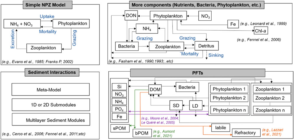
FIGURE 1. Schematic representation of the ocean biogeochemical models varying in complexity from the most basic NPZ form to those with more state variables and processes (high complexity). The labelled rectangular boxes are model variables, and processes are represented by arrows. Sediment interactions are represented which is comprised of different approaches.
Despite the importance of phytoplankton in carbon fixation in the surface ocean, direct measurements of their carbon biomass are rare, and that multiple factors, including physical processes and microbial activity, contribute to carbon export and remineralization in the oceanic carbon cycle (Hood et al., 2006). Chlorophyll (Chl-a) which is a pigment present in phytoplankton to photosynthesize is commonly used to estimate phytoplankton biomass. Chlorophyll has distinctive optical properties (Macintyre et al., 2000) and is controlled by a complex interplay of physiologic, oceanographic, and ecological ocean factors (Sverdrup, 1953; Wroblewski et al., 1988). Furthermore, the relationship between chlorophyll concentration and phytoplankton biomass is nonlinear and the ratio of chlorophyll to biomass varies by an order of magnitude under photoacclimation (Fennel, 2003; Cullen, 2015). Several biogeochemical models (Moore et al., 2002; Aumont and Bopp, 2006; Follows et al., 2007; Vichi et al., 2007), although not all of them, use a parameterization of photoacclimation to take into account changes in the phytoplankton biomass to chlorophyll ratio (Geider et al., 1997).
Along with Chl-a as being an important state variable in the biogeochemical models, macronutrients such as nitrogen, phosphorous, silica (necessary for diatom phytoplankton), and micronutrient iron play a significant role in phytoplankton growth and Chl-a production. These nutrients exist in the oceans with varying concentrations due to a variety of factors including regional variations in nutrient sources, physical processes like ocean currents and mixing, biological uptake and recycling, the impact of atmospheric deposition, and terrestrial runoff. In addition, seasonal fluctuations, upwelling events, and nutrient limitation regimes (Anderson et al., 2002; Smith, 2006; Davis et al., 2015; Yang et al., 2017) can have an impact on nutrient availability, which increases the geographical and temporal variability in nutrient concentrations across oceanic regions. Due to the increase of anthropogenic activities, coastal ecosystems receive high levels of nitrogen and phosphorous leading to eutrophication. Excessive nutrient enrichment can result in algal blooms (Chl-a concentrations above 40 g L-1) (Clarke et al., 2009). Ecosystems in various regions, such as the Baltic Sea (Vahtera et al., 2007; Rönnberg and Bonsdorff, 2016), Chesapeake Bay (Murphy et al., 2022), and the Gulf of Mexico (Rabalais et al., 2002), have experienced imbalances due to eutrophication, including oxygen depletion, loss of biodiversity, and negative effects on fish and shellfish populations.
Eutrophication can cause frequent hypoxia or anoxia (Officer et al., 1984; Naqvi et al., 2000; Soetaert and Middelburg, 2009) emphasizing the need for biogeochemical models in monitoring water quality and alerting ecosystem managers of pollution incidents (Fennel et al., 2019). These models simulate and predict fluctuations in water quality indicators, considering primary production, oxygen levels, and nutrient dynamics. By utilizing field observations and real-time monitoring data, these models can provide valuable insights to mitigate ecological imbalances promptly (Piehl et al., 2022).
In addition to macronutrients, iron is a major limiting nutrient in high latitudes seas, such as the subarctic Pacific Ocean, Southern Ocean, and southern Indian Ocean (Miller et al., 1991; Moore et al., 2004; Hamilton et al., 2020). In many regions, the atmosphere serves as the primary source of iron, which is transported as aerosols and often associated with soil dust (Fung et al., 2000; Sarthou et al., 2003). However, Iron sources can vary in different regions, including coastal Antarctica. It is essential to note that dust is not the predominant source of iron in all regions. In coastal areas, such as coastal Antarctica, diverse sources, including glacial melt and diagenesis, are considered to understand the origins of iron (Gerringa et al., 2012; Sherrell et al., 2018; Dinniman et al., 2020). Dissolved oxygen is another crucial state variable in ocean biogeochemical models, impacting the ecological and biogeochemical structure of marine ecosystems (Wilson et al., 2019). Oxygen depletion and hypoxia can occur due to factors like nutrient loading and insufficient oxygen replenishment. In regions where oxygen levels decrease significantly, known as hypoxic regions, the intensification of hypoxia leads to denitrification and the formation of oxygen minimum zones (OMZs) (Stramma et al., 2010; Stramma et al., 2009; Stramma et al., 2008; Karstensen et al., 2008; Levin and Breitburg, 2015; Lachkar et al., 2016; Lachkar et al., 2019; Lachkar et al., 2020; Levin, 2018; Grégoire et al., 2021). Coastal zones or upwelling regions are typical locations for these hypoxic regions in the ocean (Gobler and Baumann, 2016).
Biogeochemical models have been used in various ecosystems of the world ocean, and for the purpose of our study, we have classified the regions into four distinct zones: tropical, temperate, polar/subpolar, and HNLC. The tropical zone spans approximately 40% of the Earth’s surface, stretching from the Tropics of Cancer (latitude 23.5°N) to the Tropic of Capricorn (latitude 23.5°S) (Val et al., 2023). The zone is primarily defined by consistently high temperatures with a sea surface temperature above 20°C and an abundance of sunlight, which leads to high primary production and nutrient cycling. However, there may be some variation in precipitation patterns, humidity levels, and cloud cover across different regions within the tropical zone, which can influence local climate conditions (Lønborg et al., 2021). However, temperate regions are those with latitudes from 35° to 50° North and South and is marked by moderate sea surface temperatures and seasonal variations in nutrient availability and primary production (Lønborg et al., 2021). In tropical coastal waters, sea surface temperatures typically range between 20°C and 32°C. Temperate coastal waters, on the other hand, have a wider temperature range, ranging from 0°C to 25°C, with greater seasonal variation than tropical locations. Although seasonal variations are still noticeable in tropical coastal waters, they are not primarily driven by temperature (Eyre and Balls, 1999). The polar/subpolar zone is covering the Arctic and Antarctic regions (the areas between 60 degrees and the poles) and is defined by low sea surface temperatures usually range from −1°C and 14.7°, sea ice cover, and limited sunlight, leading to low primary production and nutrient cycling (Schultz, 1995). Finally, the HNLC (High Nutrient Low Chlorophyll) zones are regions where the abundance of phytoplankton biomass (or Chl-a) is low and almost constant, and macronutrients, in particular nitrates, are never considerably depleted (Edwards et al., 2004). These regions constitute more than 20% of the global ocean (Martin et al., 1994) and is found in areas where iron availability is low and limits the growth of phytoplankton, which are the base of the marine food web. The HNLC zones are found in areas of the Southern Ocean, the equatorial Pacific, and parts of the North Pacific and North Atlantic, Figure 2.
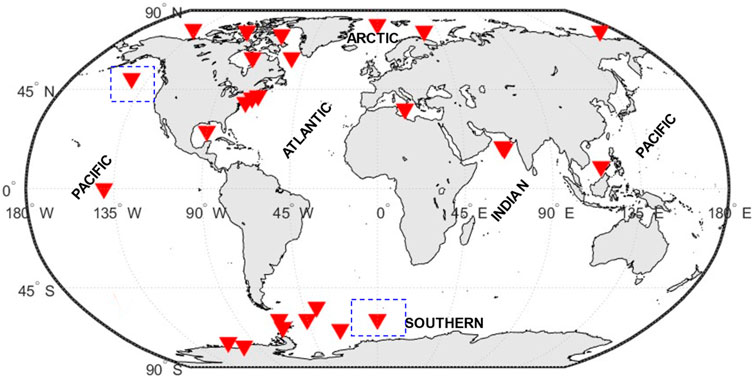
FIGURE 2. World ocean map with the indicated climatic zones presented in this study. The symbols on the map indicate regions where biogeochemical modeling studies, discussed in the review, have been conducted. Boxes with dashed outline are regions where HNLC zone mentioned in the text.
Herein, we describe existing biogeochemical models used to study various ecosystems for the present state in the global oceans at the regional and global scale, and assess their performance, strengths, uncertainties and limitations in estimating several biochemical components, including Chl-a, macronutrients (e.g., nitrate, phosphate, silicate), micronutrients (iron), carbon and oxygen cycles. This paper begins with a section that describes different modelling approaches, components, assumptions and structure. Then, the assessment of applications of these models in different ecosystems of the global oceans are discussed.
2 Biogeochemical modelling approaches
The existing biogeochemical models are categorized herein by their different level of complexity in terms of the number of phytoplankton functional types (PFTs), different forms of inorganic and organic matter, physics, and deep sediments incorporation.
2.1 Classical NPZD approach
The classical NPZD approach is an improvement of the NPZ (Evans et al., 1985; Franks, 2002) which considers a single variable for each compartment (nutrients - phytoplankton - zooplankton - detritus, sometimes including a different compartment for bacteria) neglecting the differences between the different biological types (Fasham et al., 1990; Fasham, 1993; McGillicuddy et al., 1995b). In this approach, nitrogen is typically considered a limiting nutrient because it is a necessary component of chlorophyll, nucleic acids, and proteins, all of which are important for the growth of phytoplankton and photosynthesis (Liefer et al., 2019). Also, compared to other nutrients, nitrogen availability is frequently limited, which can have an adverse effect on the entire food web by limiting phytoplankton development (Bristow et al., 2017). The detritus component accounts for the organic matter pool, which is derived from faecal materials, the fraction non-assimilated by grazing zooplankton and phytoplankton decay. The detritus is recycled by bacteria and degraded to dissolved organic nitrogen, or digested by zooplankton (Leles et al., 2016). The process through which autotrophic organisms, including phytoplankton, produce organic matter by converting sunlight and nutrients into biomass referred as primary production. Contrarily, in secondary production, organic matter is consumed by heterotrophic creatures like zooplankton, which graze on primary producers or consume other organisms.
2.2 Improving nitrogen and carbon flux and adding other elements
Modifications have been made in the classical NPZD approaches to improve the estimation of nitrogen and carbon flux (Fennel et al., 2006), with the addition of variable Chl-a and introducing a nitrogen-based nutrient-phytoplankton-heterotroph model which is of intermediate complexity with respect to Fasham’s and McGillicuddy’s models (Fasham et al., 1990; McGillicuddy et al., 1995a). Although nitrate is considered one of the most important limiting nutrients for the growth of phytoplankton biomass and primary production in open ecosystems; in some locations, such as the equatorial Pacific, North Pacific, and the Southern Ocean, nitrate (NO3) levels may exceed 4 µM (central Pacific) and phytoplankton biomass is low (Chai et al., 1996). The high nitrate and low Chl-a (HNLC) conditions observed in these regions are commonly associated with limited iron availability (Leonard et al., 1999; Pitchford and Brindley, 1999; Venables and Moore, 2010).
Nevertheless, in high-latitude areas, other factors besides the iron deficiency may also inhibit phytoplankton growth. Low temperatures (Rhee and Gotham, 1981), imbalanced nutritional stoichiometry (Gerhard et al., 2022), short days and prolonged cloud cover (ChrEilertsen and Degerlund, 2010), and grazing pressure (Dale et al., 1999) from higher trophic levels are some examples of these constraints. Leonard et al., 1999 accounted for iron limitation (nutrient compartment) in his extended NPZD model with the employment of nine compartments. The model incorporated iron partitioning into new iron and regenerated iron, as well as dissolved iron bioavailability in the marine environment. Following these developments, Galbraith developed the Biogeochemistry with Light Iron Nutrients and Gases (BLING) model, also based on NPZD (Galbraith et al., 2009). This model employs a specific approach to isolate the global impact of iron on two major features of photosynthesis: maximum light-saturated photosynthesis rates and photosynthetic efficiency. The model uses sophisticated parameterizations or algorithms to separate and quantify the impact of iron on these distinct components. These sophisticated formulations take into account various factors and processes, such as iron uptake mechanisms, iron limitation effects, and biochemical reactions, to provide a detailed understanding of how iron affects photosynthetic process. The model also considers an implicit representation (without explicitly modeling it as a separate parameter or variable) of the growth rate of phytoplankton.
The proportion of the main elements in most biogeochemical models is commonly described with a constant elemental ratio (stoichiometry): 106 C (carbon):16 N (nitrogen):1 P (phosphorous) (Redfield, 1933). This ratio is the most widely used stoichiometric reference for planktonic nutrient limitation (Ptacnik et al., 2010). Hence, biogeochemical models may consider simple growth formulations with constant C: Nutrients stoichiometry or neglect photo-acclimation by considering a constant Chl:C ratio. The classical Michaelis Menten equations are the simplest representation of phytoplankton growth (Monod, 1949) assuming a constant stoichiometric ratio between nitrogen, phosphorous, and carbon (Redfield, 1933; Ho et al., 2003; Quigg et al., 2003; Quigg et al., 2011; Finkel et al., 2006; Finkel et al., 2006). The Redfield ratio has been modified to take into account observed differences from the conventional ratio. As study by (Anderson and Sarmiento, 1994) have been conducted to analyse nutrient data and evaluate the variability of nutrient ratios under different conditions in several regions. Their research emphasizes the significance of taking into account context-specific elements that can affect nutrient stoichiometry, such as nutrient availability, microbial community composition, and ecological interactions Biogeochemical models that incorporate these modified formulations of the Redfield ratio use specific units (nitrogen, phosphorus, or carbon currency) to represent phytoplankton biomass and these models can generally be utilized for global scale studies (Aumont and Bopp, 2006; Follows et al., 2007a; Dutkiewicz et al., 2009). On the other hand (Droop, 1983), has more advanced and complex growth formulations which account for the dynamics of phytoplankton cell internal quota (Klausmeier et al., 2004; Bougaran et al., 2010; Bernard, 2011; Mairet et al., 2011; Wang et al., 2022). Thus, phytoplankton biomass in Droop’s model (Droop, 1983) is represented by at least two state variables, typically carbon and nitrogen currency. Different versions of Droop’s model have been embedded and utilized in 1D (Lancelot et al., 2000; Allen et al., 2002; Lefe et al., 2003; Mongin et al., 2003; Blackford et al., 2004; Salihoglu et al., 2008) and 3D (Tagliabue and Arrigo, 2005; Vichi et al., 2007; Vichi and Masina, 2009; Vogt et al., 2010) marine biogeochemical models. In these models, Chl-a dynamics can be also defined with various levels of complexity. The ratio of Chl: C can be constant (non-photo-acclimation), or prognostic with a dynamic behaviour (Flynn and Flynn, 1998; Geider et al., 1998; Ross and Geider, 2009) or diagnostic with an empirical (Bernard, 2011) and mechanistic relationships (Geider and Platt, 1986; Doney et al., 1996; Bissett et al., 1999). These approaches vary in terms of their level of complexity, assumptions, and underlying mechanisms employed. The constant Chl:C ratio method is the simplest, assuming no acclimation or variation in Chl-a concentration. Prognostic techniques enable dynamic modifications of the Chl-a:C ratio, capturing phytoplankton’s adaptation to changing environmental conditions. Both empirical and mechanistic diagnostic techniques estimate Chl-a content based on observational or mechanistic correlations, respectively, without explicitly modelling the physiological processes. Each method provides information about the regulation of Chl-a dynamics and their ecological implications in marine ecosystems.
Other complexities have been added to the simple NPZD model, including 1) dissolved organic nitrogen in order to allow for a comprehensive representation of a significant nitrogen pool, particularly in regions where high primary productivity is observed (Hood et al., 2001; Druon et al., 2010), 2) oxygen cycle which is known to be an essential component to represent the oxygen minimum zone caused by excessive denitrification (Naqvi et al., 2000; Codispoti et al., 2001).
2.3 Increasing the biological complexity
Unlike the simple NPZD, more complex models include different phytoplankton functional types (PFTs) and at least 15 state variables (e.g., Gregg, 2000; Gregg et al., 2003; Moore et al., 2004; Le Quéré et al., 2005; Dutkiewicz et al., 2009; Stock et al., 2014b; Wright et al., 2021; Luo et al., 2022). Considering a range of plankton groups and increasing the number of variables allows for a more thorough assessment of ecological interactions. Table 2 provides a summary of the models presented in this section, emphasizing their key characteristics and improvements. Here, we expand on the interpretation of each model improvement and discuss the relevance of increasing the number of variables.
The incorporation of Plankton Functional Types (PFTs) in biogeochemical models has been pursued to improve the accuracy of marine ecosystem representations (Anderson, 2005). Notably, the integration of additional complexity beyond NPZD models presents challenges, including limited understanding of ecology, data constraints, and the need to consolidate diversity within functional groups (Anderson, 2005). This approach is exemplified in biogeochemical models such as ERSEM (European Regional Seas Ecosystem Model) versions 1 and 2 (Baretta et al., 1995; Baretta-Bekker et al., 1997; Blackford et al., 2004). ERSEM adopts a functional role-based classification of biotic groups, categorizing phytoplankton as producers, bacteria as decomposers, and zooplankton as consumers, employing a general lower trophic approach. This approach is similar to the functional roles in an NPZD model, where each component has specific functions within the nutrient dynamics and planktonic community interactions. However, what distinguishes ERSEM from other NPZD models is its comprehensive integration of ecosystem-specific processes and interactions, allowing for a more tailored representation of biotic groups and their functions. The division of the food web into three functional categories is based on traits, including silica uptake, maximum growth rate, and nutrient affinity. The ERSEM model was initially applied to the North Sea to study the seasonal cycling of nutrients (i.e., nitrogen, phosphorous, silica, carbon). ERSEM was later modified to produce the Biogeochemical Flux Model (BFM), which accounts for the Chemical Functional Families (CFFs) in the state variables. The CFFs is split into living, non-living, and inorganic states (Vichi et al., 2007).
The Pelagic Interactions Scheme for Carbon and Ecosystem Studies (PISCES) is another example of a simple PFT model adapted from HAMOCC (Aumont et al., 2003) and extensively and widely applied in more than a hundred studies directly or indirectly (Aumont et al., 2015) The NASA Ocean Biogeochemical Model (NOBM) is a PFT model coupled with the Ocean-Atmosphere Spectral Irradiance Model (OASIM) (Gregg, 2001; Gregg et al., 2009) and is capable of simulating global-scale biogeochemical cycles. Additionally, the PlankTOM model describes the lower trophic level of marine ecosystems and has various extensions with different numbers of PFTs (Le Quéré et al., 2005; Kwiatkowski et al., 2014).
The Model of Ecosystem Dynamics, nutrient Utilization, Sequestration and Acidification (MEDUSA) includes the biogeochemical cycles of iron, silicon, and nitrogen as well as small and large plankton size classes (Yool et al., 2011; 2013). MEDUSA focuses on the biological sequestration of carbon in the deep ocean. Similarly, the Tracers of Phytoplankton with Allometric Zooplankton (TOPAZ), developed by Dunne et al., 2010, focuses on simulating the interactions among phytoplankton and allometric zooplankton, emphasizing their roles within the ecosystem dynamics.This model has been implemented in several studies (Jung, et al., 2019a; Bronselaer et al., 2020; Sharada et al., 2020) and extended in the Carbon, Ocean Biogeochemistry and Lower Trophics (COBALT) model, which improves the planktonic food web dynamics resolution to examine the influence of climate on the flow of energy from phytoplankton to fish (Stock et al., 2014a). Since the planktonic food web representation in TOPAZ is highly idealized due to an implicit representation of zooplankton and bacteria, COBALT addressed these limitations by including three explicit zooplankton groups and bacteria with a mechanistic parametrization of the impacts of these groups on the biogeochemistry (Stock et al., 2014b).
The DARWIN biogeochemical model is a more complex PFT model allowing for several different configurations and number of PFTs. It is initially developed to study Prochlorococcus species (Follows et al., 2007b) and later applied to global distributions of phytoplankton (Dutkiewicz et al., 2015; Lo et al., 2019). Nevertheless, the Regulated Ecosystem Model (REcoM) is based on a functional group approach (Schourup-Kristensen et al., 2014) and has also been commonly used in the Southern Ocean studies (Taylor et al., 2013; Losch et al., 2014; Hauck and Völker, 2015).
The complexity of the aforementioned PFT models depends on the number of the independent elements, processes parameterization (e.g., shape of functional responses, number of parameters, linear vs. nonlinear) along with the number of PFTs considered (Ford et al., 2018). As the number of PFTs increases, the complexity of the model increases as well. Generally, adding complexity to the model does not necessarily improve the model’s performance as the addition of complexity will require validation of each component of the ecosystem. Even under ideal circumstances, biogeochemical observations are lacking for full spatiotemporal coverage. As a result, the validity of additional processes is sometimes simply determined by how much they contribute to certain quantities like the total chlorophyll content (Ford et al., 2018). These studies comparing models of varying complexity have typically concluded that increasing model complexity does not always result in an increase in model skill (Friedrichs et al., 2007; Kriest et al., 2010; Ward et al., 2013; Kwiatkowski et al., 2014; Xiao and Friedrichs, 2014).
2.4 The addition of several classes of organic matter and bacteria
Bacteria play a key role in their contribution in the microbial loop, particularly in the recycling of dissolved organic matter (DOM) and provide a linkage between the higher trophic level and the dynamics of DOM (Pauer et al., 2014). In biogeochemical models studying dissolved organic matter (DOM) dynamics, various classes of organic matter, along with chemical elements and Plankton Functional Types (PFTs), have been incorporated. DOM is divided into three distinct pools based on its lability: labile DOM, semi-labile DOM, and refractory DOM. Labile DOM consists of organic molecules with a lifespan ranging from minutes to days. Semi-labile DOM undergoes decomposition over a period of 1–20 years and typically accumulates above a seasonal or permanent pycnocline. Refractory DOM, the most abundant component, exhibits the longest residence time in the water column, persisting for tens of thousands of years (Carlson and Hansell, 2015; Osterholz et al., 2015).
The ratios of DOC:DON vary among different DOM pools. The refractory DOM pool has a ratio of 3511:202, whereas the labile DOM pool has a ratio of 199:20 (Hopkinson and Vallino, 2005). These ratios indicate the relative amounts of dissolved organic carbon to dissolved organic nitrogen within each pool. It is essential to consider these ratios when incorporating DOM dynamics into biogeochemical models.
DOM in the oceans is an important input to the biogeochemical cycle, with the ocean’s DOC pool serving as the biosphere’s largest storage facility for reduced organic carbon (Hansell et al., 2009). Labile and, to a lesser extent, semi-refractory pools are driven by microbial reactions. In the microbial loop, the DOC-bacteria pathway constitutes a primary mechanism through which primary production is eitherrespired to CO2, directed to higher trophic levels, or transformed into refractory compounds. However, the refractory DOC is transported deep into the ocean (Anderson, 1999; Kahler and Koeve, 2001).
The aforementioned different forms of organic matter have been incorporated into some biogeochemical models. For instance, the semi-labile DOC and semi-labile dissolved organic nitrogen (DON) have been included in biogeochemical models that focus on regions known of their high primary productivity, particularly coastal and continental shelves regions (Druon et al., 2010; Fennel, 2010; Xue et al., 2013). These areas are potential sites for sediment denitrification and organic carbon transport to the open ocean (Devol and Christensen, 1993; Rao et al., 2007; Fennel et al., 2008; Druon et al., 2010). Another study by Schartau et al. (2007) considered the labile DOM exudation and extracellular POC formation. This process occurs during the growth of phytoplankton in which the assimilation of dissolved inorganic carbon (DIC) by phytoplankton is exuded as DOC, which is simultaneously converted into extracellular POC. A significant proportion of extracellular POC is available as transparent exopolymer particles (TEP), which consist mainly of dissolved polysaccharides (PCHO). PCHO exudation is associated with high consumption of DIC that is not directly measurable from the use of dissolved inorganic nitrogen (DIN), a phenomenon known as carbon overconsumption (Toggweiler, 1993).
2.5 Benthic-pelagic coupling
Sediment processes have been also integrated into the pelagic biogeochemical models to investigate the impact of atmospheric conditions on the ecosystem dynamics, the distribution of sediments processes in the water column, and the nitrogen budget derivation (Soetaert et al., 2001; 2000; Arthur et al., 2016; Ehrnsten et al., 2019; Kearney et al., 2020). The lack of sediment regeneration of nutrients in the biogeochemical model may lead to underestimating primary productivity (Liu et al., 2007). Adding a representation of marine sediment in biogeochemical models is important, particularly in shallow water regions like shelves, where strong vertical mixing occurs. This inclusion helps to accurately account for nutrient recycling from sediments to surface waters, preventing the underestimation of productivity (Yool et al., 2013). However, it is crucial to emphasize that in many models, sediment is represented as a boundary condition with simplistic representation, and even global models that address diagenesis frequently lack a thorough representation of the benthic ecosystem.
While incorporating sediment interactions in biogeochemical models is important to understand the linkages between sediment diagenetic processes and the global carbon cycle (Middelburg, 2018; Snelgrove et al., 2018), many models use an oversimplified representation of sediment. Several regional models have been developed to examine specific areas of the ocean at different timescales, yielding important insights into biogeochemical processes. These models such as (Soetaert et al., 2000) and the Ecological ReGional Ocean Model with vertically resolved sediments (ERGOM SED 1.0) (Radtke et al., 2019) also add to the discussion of sediment representation and its effects on oceanic and coastal ecosystems. For example, in a coastal environment (Reed et al., 2011), investigated the dynamics of sedimentary phosphorus and the development of bottom-water hypoxia. Furthermore, the relationship between sediment dynamics and biogeochemical cycling was examined by (Radtke et al., 2019).
Marine sediments representation in the biogeochemical model can be parametrized using a meta-model that is based on the downward fluxes of organic matter (Middelburg et al., 1996), a sediment box module which uses simple 1D or 2D submodules in the pelagic model to represent a simple interaction of the water column with the sedimentary pools (Yool et al., 2013), or multilayer sediment modules with chemically active sediment layers (Heinze and Maier-Reimer, 1999). Most of the biogeochemical models utilize sediment box modules or meta-models to examine eutrophication (Cerco et al., 2006; Soetaert and Middelburg, 2009; Fennel et al., 2011) or hypoxia in several regions, such as Tokyo Bay (Sohma et al., 2008), the Baltic Sea (Reed et al., 2011) and the North Sea (Lancelot et al., 2005; Meire et al., 2013).
3 Applications of biogeochemical models
The aforementioned models have been applied to resolve biochemical components including Chl-a, macronutrients (nitrogen, phosphorous, silica), micronutrients (iron), carbon and oxygen in different regions of the world’s ocean. Here, we will focus on the application of these biogeochemical models in four zones as described in the introduction section. Detailed assessments of the capabilities of these models along with their complexity through the addition of more components are provided here and summarized in Table 1. Further, the common statistical metrics for model assessment used in the analysed studies are illustrated in Table 2. To provide a comprehensive analysis of the model performance, Taylor diagrams (Taylor, 2001) are employed in various biogeochemical modelling studies. Taylor Diagrams are graphical tools that show several model performance metrics at the same time, providing an illustration of the model’s ability to capture observed data patterns. They can assist in comparing and ranking various models based on correlation, root mean square error, and standard deviation (Jolliff et al., 2009). We have added also a graphical illustration of the model’s performance separated for each zone along with their temporal scale and type of observational data used to validate the model variables, see Figures 3–7.
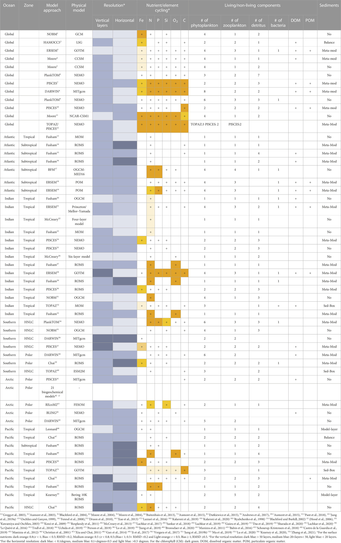
TABLE 1. Overview of the biogeochemical models reviewed in this work showing their model approach, physical model, resolution, Nutrient/element cycling, the number of the living/non-living components and sediments formulation.
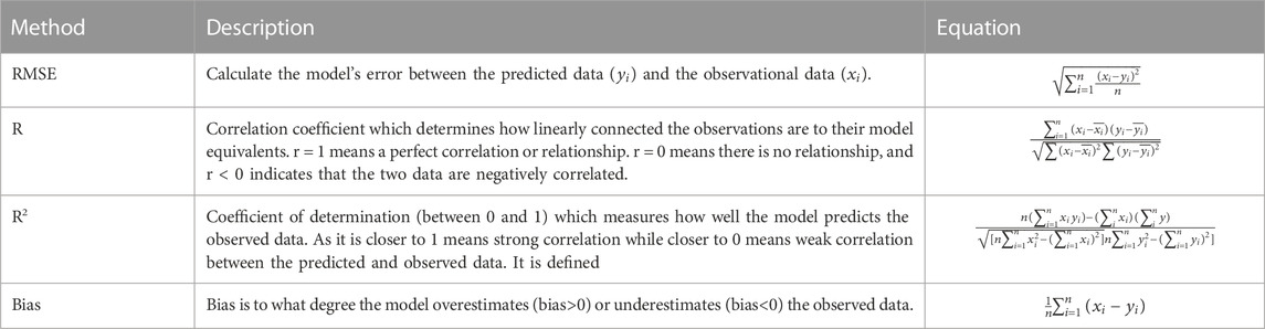
TABLE 2. The common statistical metrics for model assessment used in the analysed studies.
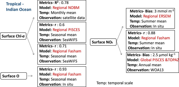
FIGURE 3. Biogeochemical variables performance for some of the models applied in the tropical ecosystems along with their temporal scale and type of observational data used to validate the model components.
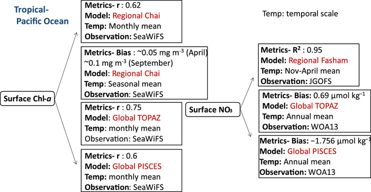
FIGURE 4. Biogeochemical variables performance for some of the models applied in the tropical Pacific ecosystems along with their temporal scale and type of observational data used to validate the model components.
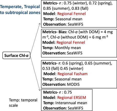
FIGURE 5. Biogeochemical variables performance for some of the models applied in the temperate, and tropical to subtropical ecosystems along with their temporal scale and type of observational data used to validate the model components.
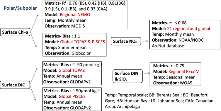
FIGURE 6. Biogeochemical variables performance for some of the models applied in the polar/subpolar ecosystems along with their temporal scale and type of observational data used to validate the model components.
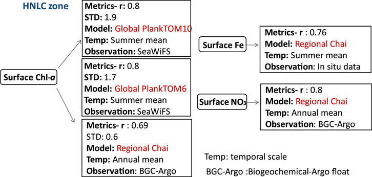
FIGURE 7. Biogeochemical variables performance for some of the models applied in the HNLC zone along with their temporal scale and type of observational data used to validate the model components.
3.1 Tropical zones
The aforementioned biogeochemical models have been applied in various tropical seas due to their high dynamism and significant biogeochemical activity, making them among the most active zones in the ocean (Lønborg et al., 2021). This section encompasses multiple regions, including the tropical Indian Ocean (specifically the Arabian Sea), the South China Sea, the tropical Pacific Ocean, and the oxygen minimum zone in the Arabian Sea. One prime example of a tropical ecosystem is the Indian Ocean, which experiences the world’s most significant monsoon system caused by the seasonal warming and cooling of massive air masses (Wiggert et al., 2005). In winter and summer, the wind patterns near the ocean change, with the southwest monsoon (SWM) providing half of the year’s wind and the northeast monsoon (NEM) providing the other half (Wiggert et al., 2005). The dynamics of the Arabian Sea’s (the most extensively studied ecosystem in the Indian Ocean) phytoplankton bloom clearly show a temporal alignment with the southwest monsoon and northeast monsoon (Madhupratap et al., 1996; Wiggert et al., 2005). Strong south-westerly winds during the summer propel coastal upwelling and offshore movement of entrained nutrients, which promote the Arabian Sea’s observed phytoplankton blooms (Brock and Mcclain, 1992; Hitchcock et al., 2000; Lierheimer and Banse, 2002). Modest north-easterly winds during the winter carry cool, dry air from the Tibetan Plateau over the northern Arabian Sea (Huang, 2010). Additionally, convective mixing during NEM entrains nutrients and promotes biological activity north of 15°N (Madhupratap et al., 1996). Thus, primary productivity and nutrients budgets in the Arabian Sea, spanning a temporal scale of seasonal variations and a spatial scale ranging from 5°S to 27°N are highly impacted by the seasonal cycle and mesoscale impacts (Resplandy et al., 2011). The primary production in terms of surface Chl-a production in the Arabian Sea is widely studied using several types of ocean biogeochemical models. For example, the estimated surface Chl-a by PISCES coupled to the Nucleus for European Modelling of the Ocean (NEMO) is compared with the weekly climatology of SeaWiFS (Sea-viewingWide Field-of-view Sensor Data). The PISCES-NEMO reproduced surface Chl-a levels of more than 0.2 mg m-3 during the NEM. It also predicted the maximum intensity of surface Chl-a, which exceeds 0.5 mg m-3, but underpredicted surface Chl-a by 30%–50% north of 20°N. This bias was found in other studies and may be attributed to the lack of diurnal layer mixing (Kawamiya and Oschlies, 2003; Wiggert et al., 2006; Koné et al., 2009). The bias in the bloom dynamics is explained by the lack of deepening of the mixed layer and nutrient feed (Wiggert et al., 2006), and light limitation (Koné et al., 2009). Another cause of inconsistencies in the PISCES model (Resplandy et al., 2011) is partially linked to the underprediction of silicate input from the Sea of Oman. PISCES captured the observed high surface Chl-a along the coasts of Somalia and southwestern India, reaching values higher than 0.4 mg m-3 during the SWM. On the other hand, it underestimated Chl-a in Oman. These inconsistencies can be attributed to the overprediction of the offshore advection by the Great Whirl and the Socotra Passage, resulting in an excessive outflow of warmer and oligotrophic waters from the Aden Gulf. Therefore, PISCES-NEMO showed better agreement with observations (seasonal SeaWiFS data) for the surface Chl-a distribution than in (Koné et al., 2009) with a correlation coefficient (r) around 0.6. These comparisons encompass a spatial scale ranging from 30°S to 30°N and from 30°E to 120°E, with a focus on seasonal variations. In addition to PISCES, the PFT model NOBM coupled with the oceanic general circulation and radiative forcing model was able to capture the intra-seasonal variability of the Indian summer monsoon, specifically focusing on the spatial scale of the Bay of Bengal (BOB) (6°–22° N; 80°–100° E) and Arabian Sea (AS) (3°–17° N; 55°–73.5° E) in the North Indian Ocean. The study showed important differences between the two regions indicating that the Arabian Sea is richer in nutrients than the Bay of Bengal with a coefficient of determination (R2) around 0.78 for the monthly mean surface Chl-a (Das et al., 2019). Furthermore, surface Chl-a is reproduced by Fasham-ROMS (Regional Ocean Modeling System), in the study region, which extends in latitude from 5°S to 30°N and in longitude from 34°E to 78°E. The performance of the model is evaluated by comparing its outputs with seasonal SeaWiFs observations, resulting in correlation coefficient ranging from 0.69 in summer to 0.74 in winter (Lachkar et al., 2017).
In addition to surface Chl-a estimation, surface nitrogen content in the Arabian Sea is estimated by the European Regional Seas Ecosystem Model (ERSEM) coupled with a 1D Princeton/Mellor–Yamada (Blackford and Burkill (2002). The model performance was assessed at three stations located at 19°N 59°E, 16°N 62°E, and 8°N 67°E, covering a seasonal timescale. The coupled model has a bias for surface nitrate concentration (3 mmol m-3) and lacks horizontal advective processes, which might be enhanced by including diurnal physical processes (horizontal advection, vertical mixing, or tidal currents). Another study by using Fasham-ROMS indicated a correlation coefficient (r) of 0.88 with observation for surface nitrate in summer. Nitrogen is not the only limiting nutrient affecting phytoplankton growth in the Arabian Sea and the ignorance of other components such as iron may underestimate nitrogen budget in the region. Iron, as an important limiting nutrient in the Arabian Sea, plays a significant role in facilitating nitrogen fixation, which is a crucial process driving biological productivity. However, nitrogen fixation is not taken into account in the NPZD, which may amplify the impact of denitrification on the nitrogen budgets in the Arabian Sea (Lachkar et al., 2017). A few studies have been conducted to examine the effect of iron limitation on global biogeochemical processes, including those in the Indian Ocean. For instance, studies using PFT approach, such as PISCES-ROMS and TOPAZ-MOM (Jung et al., 2019b) have explored the implications of iron limitation on various aspects, including macronutrient availability and ecosystem dynamics. Unlike the previous version of PISCES in (Aumont and Bopp, 2006), this version incorporated new parametrizations for iron chemistry and nitrogen fixation. PISCES exhibited a better iron estimate than TOPAZ, whereas TOPAZ showed larger bias with observation (SeaWiFS) (1.5 nMol m-3) (Jung et al., 2019b).
Another prominent feature of the Arabian Sea is its oxygen minimum zone which is noted for its low oxygen concentrations (<4 mmol/m-3) at depths of 150–1,250 m in the central part of the Arabian Sea. Thus, the dynamics of the oxygen minimum zone (OMZ) at spatial coordinates (65°E, 13°N) is studied by applying ERSEM coupled with General Ocean Turbulence Model (GOTM). The model incorporates most of the biogeochemical processes driving the dynamics of OMZ with the inclusion of denitrification process which was not considered in Butenschön et al. (2016). ERSEM-GOTM ignores the episodic intrusion of oxygen within the OMZ which may play a role in maintaining aerobic microorganisms. Therefore, the aerobic biomass within the OMZ is maintained by the residual initial conditions (Sankar et al., 2018). In addition, the model is unable to reproduce meso-zooplankton at depth, and the discrepancy between the estimates and the climatological seasonal cycles of nutrients and oxygen at depth might be due to the absence of lateral circulation in the model. Further studies on the OMZs in the Arabian Sea were investigated by Lachkar using a simple NPZD approach with the addition of the oxygen cycle (Fasham- ROMS) (Lachkar et al., 2017; Lachkar et al., 2019; Lachkar et al., 2020). Fasham-ROMS indicated that the primary productivity and OMZ are highly impacted by monsoon wind intensification, with an overall high correlation coefficient (r) 0.93 for oxygen (both seasons) in the upper layer. While the model’s horizontal grid resolution of 1/12° and vertical grid consisting of 32 sigma layers allow for some representation of eddy dynamics, the resolution may still be too coarse to fully capture all eddy processes.The OMZ intensity (oxygen concentration) has also been overestimated because of the underestimation of the northern Arabian Sea ventilation. Studies on OMZ in the Arabian Gulf are still limited.
In addition to the Indian Ocean, some parts of the Pacific Ocean are also located in the tropical zone, and south China Sea, which is the largest marginal seas of the West Pacific Ocean (Qi-zhou et al., 1994), is an example of an ecosystem that belongs to this region. Similar to the Arabian Sea, this region is largely controlled by seasonal monsoon circulation. Strong northeast (NE) winter monsoon and weaker southeast (SE) summer monsoon predominate at the sea surface of the South China Sea (SCS) (Qi-zhou et al., 1994; Li et al., 2021). Studies have shown a clear response of Chl-a and temperature of the upper oceanic conditions to atmospheric forcing in the SCS (Sun et al., 2009; Sun et al., 2010; Yang et al., 2010; Zhao et al., 2014). Estimates of the mean surface Chl-a has been reported with varying performances. A correlation coefficient (r) of 0.85 for the annual mean surface Chl-a is obtained by (Jung et al., 2019b) using both global PISCES and TOPAZ coupled to NEMO representing surface Chl-a concentration conditions (i.e., phytoplankton blooms) in the tropical Pacific. Furthermore, the monthly mean surface Chl-a was determined by PISCES-NEMO and TOPAZ-NEMO (Jung et al., 2019b) with r equal to 0.6 and 0.75, respectively. However, both models overpredicted the zonal averaged Chl-a in the Pacific Ocean east of Japan by 67%, primarily because of errors in the Kuroshio current path, as seen in low-resolution models (Gnanadesikan et al., 2002; Dutkiewicz et al., 2005; Aumont and Bopp, 2006). Nevertheless, the regional Chai’s NPZD model (Chai et al., 1996) configured for the central South China Sea was modified by adding phosphate, silicate, dissolved oxygen, DIC, two phytoplankton groups (diatoms, small phytoplankton) and their chlorophyll components (Chl1 and Chl2) has shown a correlation coefficient of approximately 0.62 for the monthly mean surface Chl-a in the SCS compared to SeaWiFS data (Ma et al., 2019). Other NPZD models were also applied in the tropical Pacific seas (SCS) to study the physical processes of mesoscale eddies’ impacts on biology such as in (Xiu and Chai, 2011). The study covered the entire Pacific Ocean, spanning from 45°S to 65°N and from 99°E to 70°W. The model exhibited a bias of approximately 0.05 mg m-3 (April) and ∼0.1 mg m-3 (September) for mean surface Chl-a concentrations when compared to SeaWiFS data for the respective months.
Other biogeochemical components such as nutrients including nitrate, phosphate, silicate, and iron have been estimated using global ocean biogeochemical models in the Pacific region. Higher positive bias for nutrients is obtained using the global TOPAZ-NEMO model compared to PISCES-NEMO in the Southern Pacific Ocean using the same physical model setup. With bias of 4.5 μmol kg−1,0.32 μmol kg−1, and 16 μmol kg−1 for nitrate, phosphate, and silicate respectively, with a higher positive bias in the central and southern Pacific for silicate (8 μmol kg−1). With regards to a NPZD based approach, Fasham-ROMS exhibited the impact of physical processes, such as lateral and vertical fluxes, as well as vertical diffusion in the shelf water, on nutrient distribution in the SCS (Ji et al., 2017; Lu et al., 2020) showing a reasonable linearity between the model estimates and field observations (JGOFS: a global, multidisciplinary program with participants from over 20 countries) for surface nitrate with R2: 0.95 (Ji et al., 2017). In (Ji et al., 2017), the model domain focused on the northwestern Pacific (NWP) region (3°–52°N, 98°–158°E), while in (Lu et al., 2020), the model domain extended from approximately 0.95°N, 99°E in the southwest corner to around 50°N, 147°E in the northeast corner.
With regards to iron, low surface concentrations of iron were predicted in the North and North Central Pacific, while high concentrations were predicted in the North and Equatorial Indian Ocean using global NOBM (Gregg et al., 2003). The model domain considered spans from approximately −84°S to 72°N latitude in increments of 1.25° longitude by 2/3° latitude. The overall correlation coefficient for the annual mean iron with in situ data is 0.86 and the reason for the iron overprediction is attributed to the lack of scavenging, excessive remineralization, and slow detritus sinking rate.
3.2 Temperate, and tropical to subtropical zones
Compared to the tropical zones, the temperate zone is characterized by moderate climate with mean annual temperatures. Average monthly air temperatures in the temperate zone typically exceed 10°C during the warmest months while water temperatures generally remain above −3°C, with a minimum around ∼-2°C. (Trewartha and Horn, 1980). In contrast, the subtropical zones, located between the tropical and temperate zones, are characterized by hot summers and moderate winters. Some parts of the North Atlantic Ocean comprises both temperate and varying tropical to subtropical zones. Biogeochemical studies in this region have focused on understanding primary productivity in continental shelves and coastal areas, which are highly productive ecosystems and are significantly influenced by human activities (Economidou, 1982; Fennel, 2010). Additionally, air-sea CO2 fluxes in coastal waters exhibit greater variability and larger amplitudes compared to fluxes in the open ocean (Tsunogai et al., 1999; Cai et al., 2003; Thomas et al., 2004). For instance, in the Mid Atlantic Bight, located in the central region of the eastern U.S. continental shelf, high primary productivity rates, sediment denitrification, and strong residual circulation contribute to the region’s significance as a potential source of organic carbon export to the open ocean (Druon et al., 2010). In the Northwest North Atlantic and other ecosystems within the region, many studies have utilized simple NPZD models to investigate the influence of physical processes on biological dynamics, rather than aiming to capture the full complexity of ecological interactions. Therefore, this section covers both coastal areas and open sea regions of the Mid Atlantic Bight, northeastern US continental shelves, Georges Bank, Gulf of Mexico, and Mediterranean waters. An example of such modeling approach is demonstrated in (Fennel et al., 2008), where the distribution of Chl-a, an indicator of productivity in the Atlantic regions, is predicted using a NPZD model. The model is coupled with a high-resolution physical model ROMS, which incorporates accurate descriptions of physical processes and an explicit representation of inorganic carbon chemistry and air-sea gas exchange of CO2 (Fennel et al., 2008). The model’s inclusion of tides in ROMS improves the seasonal mean surface Chl-a representations, showing good agreement with SeaWiFS climatology in Georges Bank (correlation coefficients: 0.75 in winter, 0.72 in spring, 0.85 in summer, and 0.83 in fall) (Fennel et al., 2008). In another study by Druon et al., 2010, Fennel’s model (Fennel et al., 2008) was further enhanced by incorporating a dissolved organic matter (DOM) module to investigate organic carbon dynamics in the North-eastern U.S. continental shelves. The model demonstrated good agreement with monthly satellite data, particularly in the inner shelf and on Georges Bank, attributing this agreement to tidal mixing and continuous nutrient suppl (Bias: Chl-a (with DOM) = 4 mg m-3, Chl-a (without DOM) = 6 mg m-3). The inclusion of the DOM module improved the model by capturing the role of dissolved organic matter in nutrient cycling and its influence on primary production in the North-eastern U.S. continental shelf. In a separate study by (Xue et al., 2013), phosphate cycling was omitted from Fennel’s model (Fennel et al., 2011) because previous studies (Rabalais et al., 2002) showed that the primary production is generally nitrogen limited in the Louisiana-Texas shelf in the Gulf of Mexico. Therefore, the correlation coefficient of the seasonal mean of simulated and observed (MODIS: Moderate Resolution Imaging Spectroradiometer) surface Chl-a for the spring, summer, fall and winter were 0.6, 0.65, 0.53, 0.45 respectively. The simulated data successfully captured the high concentration of surface Chl-a in coastal areas close to main rivers, such as the Bay of Campeche, Campeche Bank, and the Louisiana-Texas shelf, whereas Chl-a concentrations were very low in the deep ocean. It is important to note that while Louisiana/Texas shelf in the Gulf of Mexico, as discussed in Xue et al. (2013), falls outside the tropics, the Gulf of Mexico circulation does include tropical latitudes. This reference to the Gulf of Mexico was mentioned to highlight the omission of phosphate cycling in Fennel’s model due to nitrogen limitation in the primary production observed in the Louisiana-Texas shelf (Rabalais et al., 2002). In contrast to continental shelves and coastal areas of the Mid Atlantic Bight, some areas of the Atlantic Ocean and the Mediterranean Sea shows limitation of phosphate rather than nitrogen. The Mediterranean Sea encompasses the most oligotrophic ecosystems in the global ocean, with low nutrient and low chlorophyll content (Krom et al., 1991; Durrieu et al., 2011; Thingstad et al., 2014), being characterised by strong seasonality as well as highly dynamic system in terms of physics and biology (Ortenzio et al., 2009; Christaki et al., 2011). This limitation of phosphate was modelled using ERSEM which accounts for variable stoichiometric formulation in phytoplankton cells allowing the adaptation of internal N:P quota to different limiting environments (Lazzari et al., 2016). ERSEM reproduced the seasonal cycle and the observed patterns of surface Chl-a and inorganic nutrients in the Mediterranean Sea (MS). The interannual variability of Chl-a showed an agreement of r: 0.75 with SeaWiFS observation for the MS. However, the model underestimates phytoplankton blooms in the western basin of the MS while overestimates the blooms in the eastern basin during spring chlorophyll peaks. This discrepancy is attributed to the overestimation/underestimation of the winter mixing intensity by the physical model (Kalaroni et al., 2019). The spatial variability of the simulated surface Chl-a was assessed by calculating the correlation coefficient (r) between the model outputs and SeaWiFS observations. The correlation coefficient (r) was found to be 0.64, indicating a moderate positive linear association between the two datasets. The standard deviation of the spatial model variability was computed to be lower than 1 (normalised), suggesting relatively low dispersion of Chl-a values across the Mediterranean Sea. The temporal variability, on the other hand, was evaluated using unbiased root mean square differences (RMSDs) for the annual mean surface spatial and temporal variability. The RMSD value for the annual mean surface spatial variability was 0.78, indicating the average magnitude of differences between the model simulations and the observed data. Likewise, the RMSD value for the annual mean surface temporal variability was 0.68, suggesting the average magnitude of differences between the model simulations and the observed data over time. Lower RMSD values indicate better agreement in terms of both spatial and temporal variations.
3.3 Polar/subpolar and seasonally stratified zones
The effects of climate change, such as a considerable decrease in ice extent and rising sea levels, can exacerbate stratification in polar and subpolar regions (Farmer et al., 2021). In addition, changes to the global climate system are anticipated to have a significant impact on polar and subpolar marine ecosystems through their effects on water temperature and sea ice cover hence affecting marine production and carbon cycle (Gibson et al., 2020). This section covers the Arctic Ocean, Antarctic Peninsula, Drake Passage, Scotia Sea, northern Weddell Sea, South Georgia, Barents Sea, Hudson Bay, Beaufort Gyre, Labrador Sea, Baffin Bay, Canadian Arctic Archipelago, Russian shelves (East Siberian Sea), and the Dotson Ice Shelf in West Antarctica, along with the adjacent Amundsen Sea Polynya. Several ocean biogeochemical studies in the polar region focused on the effect of climate change on the carbon cycle (MCGUIRE et al., 2009; Terhaar et al., 2021; 2019; 2020; Negrete-garcía et al., 2019; Bruhwiler et al., 2021) and nutrients dynamics (Hátún et al., 2017; Randelhoff et al., 2018; 2019; Tuerena et al., 2021). Therefore, carbon is estimated using biogeochemical models with the inclusion of an explicit representation of the DIC component, such as PISCES-MIT general circulation model (MITgcm), which have been used to qualitatively examine the carbon cycle in the Arctic Ocean and have demonstrated their capacity to capture observed seasonal and regional changes in dissolved pCO2 (Manizza et al., 2011). PISCES-MITgcm represented summer levels of surface pCO2 in the Canadian Archipelago (200–250 µatm) correctly, but underestimated pCO2 spring values (∼300 µatm) relative to observations (Carbon Dioxide in the Atlantic (CARINA) data set (Jutterstrom et al., 2010)) (400–450 µatm). The lack of riverine POC and the impact of terrestrial carbon resulting from coastal erosion in the model resulted in the underprediction of the observed carbon levels. Additionally, sedimentation and resuspension processes, which may be important to enrich the water column with carbon hence impacting air-sea gas exchange, were neglected in the model. When comparing PISCES-NEMO and TOPAZ-NEMO (Jung et al., 2019b) for annual mean (averaged over all depths) DIC, TOPAZ-NEMO’s results agreed with observation (r > 0.95), and the zonally averaged surface content was better represented by TOPAZ-NEMO in the Northern Hemisphere (bias < 10 μmol kg−1). However, surface mean DIC reproduced by TOPAZ and PISCES showed a bias of −90 and 90 respectively with GLobal Ocean Data Analysis Project version 2 (GLODAPv2 (Lauvset et al., 2016)).
In addition, a modified version of Chai’s model (Chai et al., 1996) coupled to ROMS is applied over a model domain that spans the Antarctic Peninsula, Drake Passage, Scotia Sea, northern Weddell Sea, and South Georgia, indicating that dominant iron sources in the Scotia Sea are derived from sediments in the Antarctic Peninsula shelf along with the South Orkney Plateau (Jiang et al., 2019). In addition to these sources, the Antarctic Circumpolar Current, the northern side of the Weddell Gyre, upwelling, atmospheric dust deposition, and icebergs are the common sources of iron in the Southern Ocean (Jiang et al., 2019). However, the monthly means of iron levels estimated by the modified Chai’s model have shown an average overestimation by 0.26 nM, deviating from the observed average value of 0.35 nM, resulting in r: 0.76.
On the other hand, the representation of the monthly observed nitrate, mixed layer depth, as well as euphotic layer depth is reproduced in the Arctic region using a skill assessment of 21 regional and global coupled biogeochemical models based on a phytoplankton functional types, including PISCES, PlankTOM, COBALT, TOPAZ, HAMOCC, BIOMASS, MEDUSA, ERSEM, PELAGOS, PISCES and NOBM (Babin et al., 2016). Most of these models have shown a positive bias for depth-averaged nitrates, explaining the overestimation of nitrates in the upper layer (r ≤ 0.68), and none of these models were able to represent accurately the variability in field measurements (NOAA/NODC ArcNut database (Codispoti et al., 2013)). However, REcoM with its variable stoichiometry for phytoplankton’s growth and nutrient cycling (Geider et al., 1998), coupled with a high-resolution physical model: Finite Element Sea Ice-Ocean Model (FESOM), exhibited a correlation coefficient of (r = 0.75) for spatial seasonal surface values of both dissolved inorganic nitrogen (DIN) and silicate (Schourup-Kristensen et al., 2018). The simulated DIN concentration indicated low levels in the Russian shelves (East Siberian Sea) with the exception of the Lena Delta in which the nutrients are added to the water by the riverine supply.
As for the representation of Chl-a in polar ecosystems, the original version of BLING coupled with NEMO was used to study monthly high surface Chl-a levels (i.e., blooms) in the high-latitude eastern North Atlantic and the central Arctic (Castro de la Guardia et al., 2019). This model is compared with MODIS observations and showed R2: 0.76, 0.42, 0.81, 0.9, 0.1, and 0.93 in the Barents Sea (BB), Hudson Bay (HB), Beaufort Gyre (BG), Labrador Sea (LS), Baffin Bay (BB), and Canadian Arctic Archipelago (CAA) respectively. However, it underestimated the spring bloom by 1.7 mg m-3 and the fall bloom by 0.7 mg m-3 in the BB, likely because it did not take into account nutrients from riverine input. Furthermore, the model exhibited a tendency to overpredict the spring blooms in Hudson Bay (HB) and Baffin Bay (BB) by approximately 0.5 mg m-3 and 0.3 mg m-3 respectively, occurring about a month earlier than expected (March instead of April). This discrepancy might be attributed to the underprediction of sea ice concentration. Additionally, the REcoM model exhibited a bias of 1.1 mg m-3 in predicting widespread subsurface chlorophyll maxima in the central Arctic Ocean, as compared to the mean summer surface Chl-a data obtained from Globcolor observations (Schourup-Kristensen et al., 2018).
Moreover, the MITgcm-REcoM model is used to investigate the impact of sea ice on phytoplankton blooms and surface dissolved inorganic carbon (DIC) in the ocean coastal-shelf-slope ecosystem west of the Antarctic Peninsula (Schultz et al., 2019). The study area encompasses a vast region ranging from 74.7°S, 95°W in the southwest to 55°S, 55.6°W in the northeast. Simulation results were compared with ocean color observations, and research ship surveys from the Palmer Long-Term Ecological Research (LTER) program. The Palmer LTER data and MODIS/SeaWifs data showed significant discrepancies in the study of the interannual variability of the phytoplankton bloom, with correlations for surface Chl-a in different sub-regions ranging from 0.52 to 0.73. While late summer retreat years displayed positive or low negative anomalies, early sea-ice retreat years primarily displayed negative or neutral anomalies in Chl-a. The model demonstrated the influence of sea-ice dynamics on phytoplankton dynamics by indicating an earlier bloom and lower Chl-a concentrations (relative to climatology) in years with early retreat of sea ice, resulting in lower chlorophyll concentrations at the end of the summer. Conversely, in years with late retreat of sea ice, the model showed greater Chl-a concentrations later in the season. Despite discrepancies between the model and observations, the model captured the temporal shifts in bloom timing during years characterized by high or low ice extent. Additionally, the model reproduced overall seasonal anomalies in dissolved inorganic carbon (DIC), which are related to seasonal net community production (NCP).
DARWIN is another model that has been used to study regional phytoplankton distribution in the Southern Ocean (Lo et al., 2019). The model was customized to improve its accuracy by increasing the affinity of phytoplankton for nutrients, adding two distinct size classes of diatoms, and considering two different life stages for Phaeocystis (single-cell vs. colonial). These improvements increased the agreement between the simulated coccolithophore and diatom levels with the in-situ observations. However, the model inaccurately simulated monthly diatoms and haptophytes, including small non-silicified phytoplankton, in the Ross Sea. Additionally, the model overestimated small non-silicified phytoplankton in this region, resulting in a general mean absolute error for diatoms and haptophytes of 0.74 mg m−3 and 0.22 mg m−3, respectively. This inconsistency can be partially attributed to inaccuracies in representing PFT phenology and distribution, and the potential impact of iron limitation should also be considered. The representation of co-existing coccolithophores and Phaeocystis remains a challenge, and any small changes in DARWIN physiological parameters can lead to either Phaeocystis or coccolithophores loss. Furthermore, the explicit representation of sea-ice algae, which is important for accurately modeling ice-covered regions, has not been adequately incorporated.
In addition to studying Arctic and Antarctic phytoplankton dynamics, researchers have also been investigating the role of polynyas in polar ecosystems. Polynyas, which refer to expansive openings in the sea ice cover, play a crucial role in facilitating the exchange of heat, moisture, and gases between the atmosphere and the ocean (Maqueda et al., 2004; Dieckmann and Hellmer, 2009). Moreover, they drive patterns of ocean circulation, contribute to nutrient cycling, and influence ecosystem dynamics in polar regions (Maqueda et al., 2004). The rapid melting beneath the Dotson Ice Shelf (DIS) in West Antarctica, caused by warm, saline Circumpolar Deep Water (CDW) intrusions, has a significant impact on the adjacent Amundsen Sea Polynya (ASP) and its biology. Further, studies focusing on polynyas has garnered significant attention due to their substantial impact (Fichefet and Goosse, 1999; Hunke and Ackley, 2001; Wu et al., 2003). A recent study by (Twelves et al., 2020) using a coupled MITgcm-BLING model examined the effect of ice shelf melting on net primary production (NPP). The results show that melting ice shelves enhances upper ocean iron concentrations, which increases NPP. The study highlights how phytoplankton self-shading delays the bloom and reduces peak NPP while simultaneously emphasizing that changes in CDW intrusion regulate the horizontal dispersion of iron-rich meltwater, thereby impacting NPP levels.
3.4 High nutrient low chlorophyll (HNLC) zones
Biogeochemical models applied in this zone are mostly based on PFT approach which account for at least two plankton species. The section covers the Subarctic northeast Pacific at Ocean Station Papa (OSP), HNLC areas of the Southern Ocean, and the Southern Ocean (Antarctic Circumpolar Current region). Surface Chl-a concentrations are low in this region caused by iron limitation (Edwards et al., 2004). More recently (Zhang et al., 2021), used an extended version of the Chai’s model (CoSiNE-Fe) that incorporated iron cycling to investigate phytoplankton dynamics at the Ocean Station Papa (OSP) in the subarctic northeast Pacific (50°N, 145°W). The model was able to demonstrate a strong correlation between nitrate and the averaged depth-integrated Chl-a in the upper 200 m of the water column, with correlation coefficients of 0.8 and 0.69, respectively, compared to observations from a Biogeochemical-Argo float (BGC-Argo). The model’s performance was also evaluated using root-mean-square differences (RMSDs), which were 0.65 and 0.98 for nitrate and averaged depth-integrated Chl-a (in the upper 200 m), respectively.
However, the global PFT-based model PlankTOM10 coupled to NEMO was used to evaluate the role of grazing versus iron limitation in HNLC areas of the Southern Ocean (Le Quéré et al., 2016). PlankTOM10 was able to reproduce annual mean surface Chl-a estimates with a correlation coefficient (r) around 0.8 in the summer season when macro-zooplankton grazing is more intense. While this suggests that microzooplankton grazing may be a significant factor contributing to the low Chl-a concentrations observed in HNLC areas, it is important to note that high growth of phytoplankton can coexist with grazing (Lu¨rling, 2021). While both PlankTOM10 and PlankTOM6 share similar formulations, the former encompasses a greater number of plankton groups. These models yielded comparable outcomes for the annual mean surface Chl-a concentrations, demonstrating a correlation coefficient (r) of approximately 0.8 when compared with SeaWiFS satellite data. PlankTOM10, in particular, displayed slightly better performance to PlankTOM6 in terms of seasonal surface Chl-a distribution, with a bias of only 1.2%.
In contrast, DARWIN-MITgcm (Dutkiewicz et al., 2015) captured significant spatial variability in the annual mean surface Chl-a across the global oceans. Despite this, the model exhibited a relatively lower correlation coefficient of around 0.55 and tended to overestimate surface Chl-a concentration, particularly in the Southern Ocean.
Surface nitrate concentration, on the other hand, is high relative to surface Chl-a production in the HNLC zone (Edwards et al., 2004) and the global PlankTOM10 model predicted slightly lower (by 5%) of annual mean surface nitrate concentrations than observations World Ocean Atlas 2009 (Garcia et al., 2006; Le Quéré et al., 2016). Biases in the PlankTOM10 model can indeed be attributed to various limitations, including simplified overwintering strategies for zooplankton, coarse representation of iron (Fe) dynamics, the absence of certain organic matter types such as semi-refractory organic matter, and the exclusion of ecosystem pathways like viral lysis. Additionally, the model’s omission of specific zooplankton groups like salps, pteropods, and auto- and mixotrophic dinoflagellates can also contribute to biases in its predictions.
Although iron is required at low concentrations for phytoplankton growth, the lack of its sources in the HNLC zone particularly the Southern Ocean highly impact the primary productivity and phytoplankton composition. For example, in the simplified version of DARWIN biogeochemical model (Dutkiewicz et al., 2009), which consists of two species (diatoms and small phytoplankton), coupled with MITgcm model, suggested that iron supply to the surface layer of the open Southern Ocean (Antarctic Circumpolar Current region) is highly driven by eddies (Uchida et al., 2019). Eddies can improve vertical mixing, influencing the upwelling of iron from deeper waters. This transport of iron from subsurface reservoirs to the sunlit layer where phytoplankton thrive can stimulate their growth and productivity. Therefore, to improve the accuracy of iron fluxes in the Southern Ocean, it is important to consider the role of eddies in addition to the atmospheric source. In particular, the inverse energy cascade caused by meso- and sub-mesoscale baroclinic instabilities plays a crucial role in determining iron distributions (Person et al., 2019).
Additionally, a recent study by Fu (2022) which used an inverse biogeochemical model with phosphorus, carbon, and oxygen Modules (Wang et al., 2019) to investigate the effects of ocean iron fertilization (OIF) in high nutrient low chlorophyll (HNLC) regions, specifically the Southern Ocean, North Pacific, and eastern equatorial Pacific. The findings revealed that OIF led to increased productivity, causing a downward transfer of nutrients and carbon to deeper waters. This process was accompanied by improved efficiency of the soft tissue pump and an increased in the CO2 uptake. However, these positive effects were counterbalanced by a decrease in global mean oxygen levels and an expansion of oxygen minimum zones, suggesting potential consequences for ocean oxygenation and the development of hypoxic conditions. Notably, the study used (Wang et al., 2019) biogeochemical model and exhibited strong agreement with observations (GLODAPv2), showing correlation coefficients of 0.92 for dissolved inorganic phosphorus (DIP), 0.93 for dissolved inorganic carbon (DIC), and 0.85 for oxygen (O2). Interestingly, a comprehensive investigation conducted by (Bianchi et al., 2022) revealed the specific role of nitrogen cycling within the oxygen minimum zone (OMZ) of the HNLC Pacific Ocean, highlighting its implications for ecosystem dynamics. A new nitrogen cycling model was developed and specifically designed for integration into an ocean biogeochemical model, aiming to explore the impact of different nitrogen transformation processes on the biogeochemistry of the Eastern Tropical South Pacific OMZ. The model successfully captured typical OMZ conditions, providing valuable insights into the sensitivity of nitrogen transformations to environmental factors. However, it should be noted that while the model explicitly resolved N chemical tracers and their transformations, it did not directly incorporate the microbial communities responsible for these reactions, potentially limiting the understanding of the crucial role of microbes. Additionally, the model did not explicitly account for the conversion of dissolved CO2 to organic matter through chemolithotrophy due to the relatively small rates compared to organic matter remineralization in the upper ocean, posing challenges in achieving a more comprehensive integration between chemolithotrophy and the carbon cycle.
4 Limitations and future developments
Although the aforementioned biogeochemical models performed well in several ecosystems, they have been modified and improved over the years by incorporating more components and processes to improve their reliability and predictability. Even in the most recent and advanced biogeochemical research, however, some limits remain. This section discusses the limitations of the existing biogeochemical models applied in several oceans, as well as recommendations for future modeling studies.
The absence of viruses in current biogeochemical models is a noteworthy drawback that demands more attention. Viruses play an important role in marine ecosystems by controlling microbial population numbers and altering the dynamics of nutrient and carbon cycling (Weitz and Wilhelm, 2012; Mateus, 2017). Their ability to infect and lyse bacteria and other microbes leads to the release of intracellular organic materials, which other species can then uptake (Zhao et al., 2019). Incorporating viruses into biogeochemical models may help us gaining a deeper understanding of how ecosystems work and the complex connections that exist between the different components of the microbial community (Weitz et al., 2015). These models may more accurately represent the intricate feedback systems that control nutrient availability, primary productivity, and carbon sequestration in the oceans by taking the viral impact into account. Furthermore, viruses can alter the variety and dominance of species by profoundly altering the structure and makeup of microbial communities (Tran and Anantharaman, 2021). Their impact on community dynamics and adaptability to environmental changes emphasizes how crucial they are in determining the stability and resiliency of the ecosystem.
In addition to not properly representing viruses, biogeochemical models often neglect the inclusion of archaea, despite their important role in ammonia oxidation processes. Archaea are important in ammonia oxidation and have the ability to affect nitrogen cycling, according to studies by (Urakawa et al., 2010; Yakimov et al., 2011). Similarly, mixotrophs, organisms capable of both photosynthetic and heterotrophic feeding, are often overlooked in biogeochemical models. Studies by (Stoecker et al., 2017; Edwards, 2019; Faure et al., 2019; Wilken et al., 2019) have revealed mixotrophs’ ecological importance and possible impact on nutrient dynamics and ecosystem functioning. Unfortunately, most models do not treat mixotrophs as distinct Plankton Functional Types (PFTs), limiting our understanding of their contributions.
Furthermore, autotrophic bacteria such as nitrifying bacteria which carry out two-step nitrification processes are oversimplified in many biogeochemical models. These types of bacteria compete with the photosynthesizers for inorganic carbon and their current representation may underestimate or overestimate the primary productivity in the ocean. In addition, the detritus component is not well classified in many marine biogeochemical models and the representation of organic matter is not fully considered, leading to a possible under/overestimation of organic matter. Although the most intricate models include more components, they omit some important processes, including day-night cycles, zooplankton’s diurnal migration (Ford et al., 2018). The omission of fish from biogeochemical models represent another significant area that needs exploration. Fish play an important part in the recycling and regeneration of nutrients within marine environments (Mcintyre et al., 2007). Thus, incorporating their interactions with other ecosystem components, such as feeding patterns and nutrient excretion, would provide valuable insights into nutrient dynamics and enhance our understanding of ecosystem functioning. Furthermore, the omission or simplification of benthic (e.g., Lazzari et al., 2016; Kalaroni et al., 2020) and sea ice components in biogeochemical models can hinder accurate predictions of ecosystem responses to environmental changes, thereby affecting the carbon and nutrient cycling assessment.
Biogeochemical models commonly simplify the representation of nitrogen (N) transformations, failing to capture the complexity of the underlying network of N reactions and their controlling factors. In the case of N2O cycling, many models rely on oversimplified parameterizations that consider N2O production solely from nitrification or aerobic respiration, while neglecting the important N2O sources and sinks associated with denitrification (Suntharalingam and Sarmiento, 2000; Jin and Gruber, 2003; Nevison et al., 2003; Manizza et al., 2012). The comprehensive consideration of nitrite cycling in the presence of low oxygen conditions, encompassing the concurrent processes of nitrite production from nitrate dissimilatory reactions, reduction to N2O and N2 via denitrification and anammox, and subsequent reoxidation to nitrate, is insufficiently addressed (Lam and Kuypers, 2011; Kalvelage et al., 2013; Babbin et al., 2014; Babbin et al., 2015; Buchwald et al., 2015; Babbin et al., 2017).
In summary, although many biogeochemical models are able to simulate certain phenomenon/conditions, in certain regions of the global oceans they may underpredict/overpredict concentrations of some components that can be largely dependent on other missing elements mentioned above. Therefore, biogeochemical models could be improved through the inclusion of dissolved organic carbon (labile, semi-labile, refractory), mixotrophic functional groups, viruses which in turn improve the representation of plankton functional groups, heterotrophic and microbial food web. While assessing biogeochemical models for current conditions reveals model biases, it does not always explain how they behave outside of the observed conditions (Fennel et al., 2022). Nevertheless, adding complexity does not always guarantee improved model performance or changes in rates. For example, Luo et al. (2022) found that while the drivers of export rate can change with the addition of an extra zooplankton component like tunicates, the total export amount may not vary significantly.
Obtaining comprehensive and high-quality data for model initialization and parameterization continues to be a challenge, with limited accessible sources available. Moreover, the challenges associated with data acquisition in polar regions make it difficult to effectively compare models with the available data. These challenges are primarily related to factors such as sea ice and cloud cover, which often result in substantial gaps in the coverage of remote sensing data.
Improvement in the zooplankton component may help further in constraining processes that regulate Chl-a distribution in the models (Clerc et al., 2021; Ratnarajah et al., 2023). Moreover, re-considering simulations of under-ice and near-ice phytoplankton blooms in the cold ecosystems by defining the photosynthesis irradiance curve for each phytoplankton group and allowing seasonal plasticity in the model parameters may increase the reliability of models applied in Arctic regions (Kearney et al., 2020). Most of the current models use a simplified, single-size detritus component, but in fact, detritus consists of different sizes and sinking rates, which may result in significant limitations in some regions (Ford et al., 2018). Considering different types of detrital matter with various timescales in the remineralization process would produce a more realistic model output for the organic matter.
5 Conclusion
This review presents different biogeochemical models applied to various ecosystems of the world’s ocean. Most of these widely used ocean biogeochemical models are an extension of NPZD models and have undergone several modifications and developments which increased their complexity in terms of number of PFTs, organic matter, physics, and sediments interactions. We divided the oceans into four zones, tropical, temperate and varying from tropical to subtropical, polar/subpolar, and HNLC zones to review the biogeochemical modelling studies been done on the biogeochemical components in these regions separately. Estimation of biogeochemical model variables, such as Chl-a, nutrients, carbon and oxygen in various ecosystems have shown varying performances. The varying performances for these biogeochemical model variables are dependent on the features of the ecosystems and the resolution of the physical environment. In the tropical and subtropical ecosystems, seasonal variations are highly strong and have a great impact on the biogeochemical cycles in these regions. These regions are known to be the most productive ecosystems in the ocean and nutrients can be supplied to the open ocean from the coastal enriched nutrients. Due to considerable decrease in ice extent and rising sea levels caused by climate change, the Arctic/Antarctic region experiences rapid changes in the physical and biological ecosystems. This is observed in the changes of the Arctic carbon and nutrients cycles. Ocean biogeochemical models play a critical role in climate studies, particularly in regions that are prone to experiencing high variations in extreme climates. The increase in carbon and nitrogen concentrations in the biosphere, resulting from anthropogenic activities, has the potential to disrupt biogeochemical cycles. This alteration of biogeochemical cycles can have wide-ranging impacts, making biodiversity, food security, and water quality more susceptible to the impacts of climate change.
Author contributions
KI and MA-S defined the content of the manuscript. KI prepared the manuscript and MA-S contributed in conceptualization, revisions and improvements. All authors contributed to the article and approved the submitted version.
Acknowledgments
The authors would like to thank Khalifa University for the financial support. This paper is under the project of modelling the biogeochemistry of the Arabian Gulf waters.
Conflict of interest
The authors declare that the research was conducted in the absence of any commercial or financial relationships that could be construed as a potential conflict of interest.
Publisher’s note
All claims expressed in this article are solely those of the authors and do not necessarily represent those of their affiliated organizations, or those of the publisher, the editors and the reviewers. Any product that may be evaluated in this article, or claim that may be made by its manufacturer, is not guaranteed or endorsed by the publisher.
References
Achterberg, E. P. (2014). Grand challenges in marine biogeochemistry. Front. Mar. Sci. 1, 1–5. doi:10.3389/fmars.2014.00007
Allen, J. I., Somerfield, P. J., and Siddorn, J. (2002). Primary and bacterial production in the Mediterranean Sea: a modelling study. J. Mar. Syst. 34, 473–495. doi:10.1016/s0924-7963(02)00072-6
Anderson, L. A., and Sarmiento, J. L. (1994). Redfield ratios of remineralization determined by nutrient data analysis. Glob. Biogeochem. Cycles 8, 65–80. doi:10.1029/93gb03318
Anderson, R., and Williams, P. J. l. B. (1999). A one-dimensional model of dissolved organic carbon cycling in the water column incorporating combined biological-photochemical decomposition. Refract. Mater. Amador 13, 337–349. doi:10.1029/1999gb900013
Anderson, T. R. (2005). Plankton functional type modelling: running before we can walk. J. Plankton Res. 27, 1073–1081. doi:10.1093/plankt/fbi076
Andrews, O., Buitenhuis, E., Le Quéré, C., and Suntharalingam, P. (2017). Biogeochemical modelling of dissolved oxygen in a changing ocean. Phil. Trans. R. Soc. A 375, 20160328. doi:10.1098/rsta.2016.0328
Anderson, D. M., Patricia, G., and Burkholder, J. M. (2002). Harmful algal blooms and eutrophication: nutrient sources, composition, and consequences. Estuaries 25, 704–726. doi:10.1007/BF02804901
Arthur, C., Ioanna, A., Karline, S., Ioanna, A., and Karline, S. (2016). Integrating sediment biogeochemistry into 3D oceanic models: a study of benthic-pelagic coupling in the black sea. Ocean. Model 101, 83–100. doi:10.1016/j.ocemod.2016.03.006
Aumont, O., and Bopp, L. (2006). Globalizing results from ocean in situ iron fertilization studies. Glob. Biogeochem. Cycles 20, 1–15. doi:10.1029/2005GB002591
Aumont, O., Ethé, C., Tagliabue, A., Bopp, L., and Gehlen, M. (2015). PISCES-v2: an ocean biogeochemical model for carbon and ecosystem studies. Geosci. Model Dev. Discuss. 8, 1375–1509. doi:10.5194/gmdd-8-1375-2015
Aumont, O., Maier-Reimer, E., Blain, S., and Monfray, P. (2003). An ecosystem model of the global ocean including Fe, Si, P colimitations. Glob. Biogeochem. Cycles 17, 1745. doi:10.1029/2001gb001745
Babbin, A. R., Bianchi, D., Jayakumar, A., and Ward, B. B. (2015). Rapid nitrous oxide cycling in the suboxic ocean. Sci. (80-. ) 348, 1127–1129. doi:10.1126/science.aaa8380
Babbin, A. R., Keil, R. G., Devol, A. H., and Ward, B. B. (2014). Organic matter stoichiometry, flux, and oxygen control nitrogen loss in the Ocean. Sci. (80-. ) 344, 406–408. doi:10.1126/science.1248364
Babbin, A. R., Peters, B. D., Casciotti, K. L., Ward, B. B., and Widner, B. (2017). Multiple metabolisms constrain the anaerobic nitrite budget in the Eastern Tropical South Pacific. Glob. Biogeochem. Cycles 31, 258–271. doi:10.1002/2016GB005407
Babin, M., Buitenhuis, E. T., Chevallier, M., Mora, L. D., and Dessert, M. (2016). Net primary productivity estimates and environmental variables in the Arctic Ocean. Assess. coupled physical-biogeochemical models 2016, 1–35. doi:10.1002/2016JC011993
Baretta, J. W., Ebenhöh, W., and Ruardij, P. (1995). The European regional seas ecosystem model, a complex marine ecosystem model. Neth. J. Sea Res. 33, 233–246. doi:10.1016/0077-7579(95)90047-0
Baretta-Bekker, J. G., Baretta, J. W., and Ebenhöh, W. (1997). Microbial dynamics in the marine ecosystem model ERSEM II with decoupled carbon assimilation and nutrient uptake. J. Sea Res. 38, 195–211. doi:10.1016/S1385-1101(97)00052-X
Bernard, O. (2011). Hurdles and challenges for modelling and control of microalgae for CO 2 mitigation and biofuel production. IFAC 43, 667–678. doi:10.3182/20100705-3-BE-2011.00111
Bianchi, D., Mccoy, D., and Yang, S. (2022). Formulation, optimization and sensitivity of NitrOMZv1. 0, a biogeochemical model of the nitrogen cycle in oceanic oxygen minimum zones. Geosci. Model Dev. 16 (12), 3581–3609. doi:10.5194/gmd-16-3581-2023
Bissett, W. P., Walsh, J. J., Dieterle, D. A., and Carder, K. L. (1999). Carbon cycling in the upper waters of the sargasso sea: i. numerical simulation of differential carbon and nitrogen fluxes. Deep. Res. Part I Oceanogr. Res. Pap. 46, 205–269. doi:10.1016/S0967-0637(98)00062-4
Blackford, J. C., Allen, J. I., and Gilbert, F. J. (2004). Ecosystem dynamics at six contrasting sites: a generic modelling study. J. Mar. Syst. 52, 191–215. doi:10.1016/j.jmarsys.2004.02.004
Blackford, J. C., and Burkill, P. H. (2002). Planktonic community structure and carbon cycling in the Arabian Sea as a result of monsoonal forcing: the application of a generic model. J. Mar. Syst. 36, 239–267. doi:10.1016/S0924-7963(02)00182-3
Bougaran, G., Bernard, O., and Sciandra, A. (2010). Modeling continuous cultures of microalgae colimited by nitrogen and phosphorus. J. Theor. Biol. 265, 443–454. doi:10.1016/j.jtbi.2010.04.018
Bristow, L. A., Mohr, W., Ahmerkamp, S., and Kuypers, M. M. M. (2017). Nutrients that limit growth in the ocean. Curr. Biol. 27, R474–R478. doi:10.1016/j.cub.2017.03.030
Brock, J. C., and Mcclain, C. R. (1992). Interannual variability in phytoplankton blooms observed in the northwestern Arabian Sea during the southwest monsoon. J. Geophys. Res. Oceans 97, 733–750. doi:10.1029/91JC02225
Bronselaer, B., Russell, J. L., Winton, M., Williams, N. L., Key, R. M., Dunne, J. P., et al. (2020). Importance of wind and meltwater for observed chemical and physical changes in the Southern Ocean. Nat. Geosci. 13, 35–42. doi:10.1038/s41561-019-0502-8
Bruhwiler, L., Parmentier, F.-J. W., Crill, P., Leonard1, M., and Palmer, P. I. (2021). The arctic carbon cycle and its response to changing climate. Curr. Clim. Chang. Rep. 7, 14–34. doi:10.1007/s40641-020-00169-5
Buchwald, C., Santoro, A. E., Stanley, R. H. R., and Casciotti, K. L. (2015). Global biogeochemical cycles of the eastern tropical north paci fi c off Costa Rica. Glob. Biogeochem. Cycles 2015, 2061–2081. doi:10.1002/2015GB005187
Butenschön, M., Clark, J., Aldridge, J. N., Icarus Allen, J., Artioli, Y., Blackford, J., et al. (2016). ERSEM 15.06: a generic model for marine biogeochemistry and the ecosystem dynamics of the lower trophic levels. Model Dev. 9, 1293–1339. doi:10.5194/gmd-9-1293-2016
Buitenhuis, E. T., Hashioka, T., and Quéré, C. Le. (2013). Combined constraints on global ocean primary production using observations and models. Glob. Biogeochem. Cycles 27 (3), 847–858. doi:10.1002/gbc.20074
Cai, W., Wang, Z. A., and Wang, Y. (2003). The role of marsh-dominated heterotrophic continental margins in transport of CO2between the atmosphere, the land-sea interface and the ocean: the role of marsh-dominated heterotrophic continental margins. Geophys. Res. Lett. 30 (16), 1849. doi:10.1029/2003GL017633
Carlson, C. A., and Hansell, D. A. (2015). DOM sources, sinks, reactivity, and budgets. Biogeochem. Mar. Dissolved Org. Matter 2015, 65–126. doi:10.1016/B978-0-12-405940-5.00003-0
Castro de la Guardia, L., Garcia-Quintana, Y., Claret, M., Hu, X., Galbraith, E. D., and Myers, P. G. (2019). Assessing the role of high-frequency winds and Sea Ice loss on arctic phytoplankton blooms in an Ice-Ocean-biogeochemical model. J. Geophys. Res. Biogeosciences 124, 2728–2750. doi:10.1029/2018JG004869
Cerco, C. F., Noel, M. R., and Kim, S. C. (2006). Three-dimensional management model for lake Washington, Part II: eutrophication modeling and skill assessment. Lake Reserv. Manag. 22, 115–131. doi:10.1080/07438140609353889
Chai, F., Lindley, S. T., and Barber, R. T. (1996). Origin and maintenance of a high nitrate condition in the equatorial Pacific. Deep. Res. Part II Top. Stud. Oceanogr. 43, 1031–1064. doi:10.1016/0967-0645(96)00029-X
Cherif, M., and Loreau, M. (2010). Towards a more biologically realistic use of Droop ’ s equations to model growth under multiple nutrient limitation. Oikos 119 (6), 897–907. doi:10.1111/j.1600-0706.2010.18397.x
Christian, J. R., Verschell, M. A., Murtugudde, R., Busalacchi, A. J., and McClain, C. R. (2001). Biogeochemical modelling of the tropical Pacific Ocean. I: Seasonal and interannual variability. Deep-Sea Res. Part I Top. Stud. Oceanogr. 49 (1–3), 509–543. doi:10.1016/S0967-0645(01)00110-2
ChrEilertsen, H., and Degerlund, M. (2010). Phytoplankton and light during the northern high-latitude winter. J. Plankton Res. 32 (6), 899–912. doi:10.1093/plankt/fbq017
Christaki, U., Wambeke, F., Lagaria, A., Prieur, L., Grattepanche, J., Pujo-Pay, M., et al. (2011). Microbial food webs and metabolic state across oligotrophic waters of the Mediterranean Sea during summer. Biogeosciences 8, 1839–1852. doi:10.5194/bg-8-1839-2011
Clarke, R. A., Stanley, C. D., Macleod, B. W., and Mcneal, B. L. (2009). Relationship of seasonal water quality to chlorophyll a concentration in lake manatee, Florida. Lake Reserv. Manag. 13, 253–258. doi:10.1080/07438149709354316
Clerc, C., Aumont, O., and Bopp, L. (2021). Should we account for mesozooplankton reproduction and ontogenetic growth in biogeochemical modeling. Theor. Ecol. 14, 589–609. doi:10.1007/s12080-021-00519-5
Codispoti, L. A., Brandes, J. A., Christensen, J. P., Devol, A. H., Naqvi, S. W. A., Paerl, H. W., et al. (2001). The oceanic fixed nitrogen and nitrous oxide budgets: moving targets as we enter the anthropocene? Sci. Mar. 65, 85–105. doi:10.3989/scimar.2001.65s285
Codispoti, L. A., Kelly, V., Thessen, A., Matrai, P., Suttles, S., Hill, V., et al. (2013). Synthesis of primary production in the Arctic Ocean: 3 Nitrate and phosphate based estimates of net community production. Prog. Oceanogr. 110, 126–150. doi:10.1016/j.pocean.2012.11.006
Cox, P. M., Betts, R. A., Jones, C. D., Spall, S. A., and Tollerdell, I. J. (2000). Erratum: acceleration of global warming due to carbon-cycle feedbacks in a coupled climate model. Nature 408, 750. doi:10.1038/35047138
Cullen, J. J. (2015). Subsurface chlorophyll maximum layers: enduring enigma or mystery solved. Ann. Rev. Mar. Sci. 7, 207–239. doi:10.1146/annurev-marine-010213-135111
Dale, T., Rey, F., and Heimdal, B. R. (1999). Seasonal development of phytoplankton at a high latitude oceanic site. Sarsia 84, 419–435. doi:10.1080/00364827.1999.10807347
Das, D., Chakrabarty, M., Goswami, S., Basu, D., and Chaudhuri, S. (2019). Impact of intra-seasonal oscillations of Indian summer monsoon on biogeochemical constituents of North Indian Ocean. Theor. Appl. Climatol. 136, 839–848. doi:10.1007/s00704-018-2518-1
Davis, T. W., Bullerjahn, G. S., Tuttle, T., Mckay, R. M., and Watson, S. B. (2015). Effects of increasing nitrogen and phosphorus concentrations on phytoplankton community growth and toxicity during planktothrix blooms in sandusky Bay, lake erie. Lake Erie 4840 South State Road. 49, 7197–7207. doi:10.1021/acs.est.5b00799
Devol, A. H., and Christensen, J. P. (1993). Benthic fluxes and nitrogen cycling in sediments of the continental margin of the eastern North Pacific. J. Mar. Res. 51, 345–372. doi:10.1357/0022240933223765
Dieckmann, G. A., and Hellmer, H. (2009). “The importance of sea ice: an overview,” in Sea ice. Editors D. N Thomas, and G. S Dieckmann. second ed (Oxford: Wiley-Blackwell, Wiley-Blackwell), 1–22.
Dinniman, M. S., St-laurent, P., Arrigo, K. R., Hofmann, E. E., and Dijken, G. L. V. (2020). Analysis of iron sources in antarctic continental shelf waters. Analysis Iron Sources Antarct. Cont. Shelf Waters 125, 2019jc015736. doi:10.1029/2019jc015736
Doney, S. C., Glover, D. M., and Najjar, R. G. (1996). A new coupled, one-dimensional biological-physical model for the upper ocean: applications to the JGOFS Bermuda Atlantic Time-series study (BATS) site. Deep. Res. Part II Top. Stud. Oceanogr. 43, 591–624. doi:10.1016/0967-0645(95)00104-2
Droop, M. R. (1983). 25 Years of algal growth kinetics A personal view. Bot. Mar. XXVI 26, 99–112. doi:10.1515/botm.1983.26.3.99
Droop, M. R. (1973). Some thoughts on nutrient limitation in algae. J. Phycol. 9, 264–272. doi:10.1111/j.1529-8817.1973.tb04092.x
Druon, J. N., Mannino, A., Signorini, S., McClain, C., Friedrichs, M., Wilkin, J., et al. (2010). Modeling the dynamics and export of dissolved organic matter in the Northeastern U.S. continental shelf. Estuar. Coast. Shelf Sci. 88, 488–507. doi:10.1016/j.ecss.2010.05.010
Dunne, J., Gnanadesikan, A., Sarmiento, J. L., Slater, R. D., and Hiscock, M. R. (2010). Efficiency of small scale carbon mitigation by patch iron fertilization. Biogeosciences Suppl. 7, 3593–3624. doi:10.5194/bg-7-3593-2010
Durrieu, G. X., Madron, D., Guieu, C., Sempéré, R., Conan, P., Cossa, D., et al. (2011). Marine ecosystems’ responses to climatic and anthropogenic forcings in the Mediterranean. Prog. Oceanogr. 91, 97–166. doi:10.1016/j.pocean.2011.02.003
Dutkiewicz, S., Baird, M., and Chai, F. (2020). Synergy between ocean colour and biogeochemical/ecosystem models.
Dutkiewicz, S., Follows, M. J., and Bragg, J. G. (2009). Modeling the coupling of ocean ecology and biogeochemistry. Glob. Biogeochem. Cycles 23, 1–15. doi:10.1029/2008GB003405
Dutkiewicz, S., Follows, M. J., and Parekh, P. (2005). Interactions of the iron and phosphorus cycles: a three-dimensional model study. Glob. Biogeochem. Cycles 19, 1–22. doi:10.1029/2004GB002342
Dutkiewicz, S., Hickman, A. E., Jahn, O., Gregg, W. W., Mouw, C. B., and Follows, M. J. (2015). Capturing optically important constituents and properties in a marine biogeochemical and ecosystem model. Biogeosciences 12, 4447–4481. doi:10.5194/bg-12-4447-2015
Economidou, E. (1982). The ecological value of coastal ecosystems coastal ecosystems. Ekistics 49, 98–101.
Edwards, A. M., Platt, T., and Sathyendranath, S. (2004). The high-nutrient, low-chlorophyll regime of the ocean: limits on biomass and nitrate before and after iron enrichment. Ecol. Model. 71, 103–125. doi:10.1016/j.ecolmodel.2003.06.001
Edwards, K. F. (2019). Mixotrophy in nanoflagellates across environmental gradients in the ocean. Mix. nanoflagellates across Environ. gradients ocean 116, 6211–6220. doi:10.1073/pnas.1814860116
Ehrnsten, E., Norkko, A., Timmermann, K., and Gustafsson, B. G. (2019). Benthic-pelagic coupling in coastal seas – modelling macrofaunal biomass and carbon processing in response to organic matter supply. J. Mar. Syst. 196, 36–47. doi:10.1016/j.jmarsys.2019.04.003
Evans, G. T., Parslow, J. S., Evans, G. T., and Parslow, J. S. (1985). A model of annual plankton cycles. Deep Sea Research Part B. Oceanogr. Lit. Rev. 32 (9), 759. doi:10.1016/0198-0254(85)92902-4
Eyre, B., and Balls, P. (1999). A Comparative Study of Nutrient Behavior along the Salinity Gradient of Tropical and Temperate Estuaries REFERENCES Linked references are available on JSTOR for this article: you may need to log in to JSTOR to access the linked references. A Comp. 22, 313–326. doi:10.2307/1352987
Farmer, J. R., Sigman, D. M., Granger, J., Underwood, O. M., Fripiat, F., Cronin, T. M., et al. (2021). Arctic Ocean stratification set by sea level and freshwater inputs since the last ice age. Nat. Geosci. 14, 684–689. doi:10.1038/s41561-021-00789-y
Fasham, M. J. R., Ducklow, H. W., and McKelvie, S. M. (1990). A nitrogen-based model of plankton dynamics in the oceanic mixed layer. J. Mar. Res. 48, 591–639. doi:10.1357/002224090784984678
Fasham, M. J. R. (1993). Modelling the marine biota. Glob. Carbon Cycle, I 1993, 457–504. doi:10.1007/978-3-642-84608-3_19
Faure, E., Not, F., Benoiston, A.-S., Labadie, K., Bittner, L., and Ayata, S.-D. (2019). Mixotrophic protists display contrasted biogeographies in the global ocean. ISME J. 13, 1072–1083. doi:10.1038/s41396-018-0340-5
Fennel, K., and Boss, E. (2003). Subsurface maxima of phytoplankton and chlorophyll: steady-state solutions from a simple model. Limnol. Oceanogr. 48, 1521–1534. doi:10.4319/lo.2003.48.4.1521
Fennel, K., Gehlen, M., Brasseur, P., Brown, C. W., Ciavatta, S., Cossarini, G., et al. (2019). Advancing marine biogeochemical and ecosystem reanalyses and forecasts as tools for monitoring and managing ecosystem health. Front. Mar. Sci. 6, 1–9. doi:10.3389/fmars.2019.00089
Fennel, K., Hetland, R., Feng, Y., and DiMarco, S. (2011). A coupled physical-biological model of the northern Gulf of Mexico shelf: model description, validation and analysis of phytoplankton variability. Biogeosciences Discuss. 8, 121–156. doi:10.5194/bgd-8-121-2011
Fennel, K., Mattern, J. P., Doney, S. C., Bopp, L., Moore, A. M., Wang, B., et al. (2022). Ocean biogeochemical modelling. Nat. Rev. 2, 76. doi:10.1038/s43586-022-00154-2
Fennel, K. (2010). The role of continental shelves in nitrogen and carbon cycling: northwestern North Atlantic case study. Ocean. Sci. 6, 539–548. doi:10.5194/os-6-539-2010
Fennel, K., Wilkin, J., Levin, J., Moisan, J., O’Reilly, J., and Haidvogel, D. (2006). Nitrogen cycling in the middle atlantic Bight: results from a three-dimensional model and implications for the North Atlantic nitrogen budget. Glob. Biogeochem. Cycles 20, 20. doi:10.1029/2005GB002456
Fennel, K., Wilkin, J., Previdi, M., and Najjar, R. (2008). Denitrification effects on air-sea CO2 flux in the coastal ocean: simulations for the northwest North Atlantic. Geophys. Res. Lett. 35, L24608. doi:10.1029/2008GL036147
Fichefet, T., and Goosse, H. (1999). A numerical investigation of the spring Ross Sea polynya. A Numer. investigation spring Ross Sea polynya 26, 1015–1018. doi:10.1029/1999gl900159
Finkel, Z. V., Quigg, A., Raven, J. A., Schofield, O. E., and Falkowski, P. G. (2006). Irradiance and the elemental stoichiometry of marine phytoplankton. Irradiance Elem. Stoichiom. Mar. Phytoplankt. 51, 2690–2701. doi:10.4319/lo.2006.51.6.2690
Flynn, K. J., and Flynn, K. (1998). Release of nitrite by marine dinoflagellates: development of a mathematical simulation. Mar. Biol. 130, 455–470. doi:10.1007/s002270050266
Follows, M. J., Dutkiewicz, S., Grant, S., and Chisholm, S. W. (2007a). Emergent biogeography of microbial communities in a model ocean. Science 80, 1843–1846. doi:10.1126/science.1138544
Follows, M. J., Dutkiewicz, S., Grant, S., and Chisholm, S. W. (2007b). Emergent biogeography of microbial communities in a model ocean. Sci. (80-. ) 315, 1843–1846. doi:10.1126/science.1138544
Ford, D., Kay, S., McEwan, R., Totterdell, I., and Gehlen, M. (2018). Marine biogeochemical modelling and data assimilation for operational forecasting, reanalysis, and climate research. New Front. Oper. Oceanogr. 2018, 625–652. doi:10.17125/gov2018.ch22
Franks, P. (2002). NPZ Models of Plankton Dynamics: Their construction,coupling with physics, and application.
Friedrichs, M. A. M., Dusenberry, J. A., Anderson, L. A., Armstrong, R. A., Chai, F., Christian, J. R., et al. (2007). Assessment of skill and portability in regional marine biogeochemical models: role of multiple planktonic groups. J. Geophys. Res. Ocean. 112, C08001. doi:10.1029/2006JC003852
Fung, I. Y., Meyn, S. K., Tegen, I., Doney, S. C., John, J. G., and Bishop, J. K. B. (2000). Iron supply and demand in the upper ocean. Glob. Biogeochem. Cycles 14, 281–295. doi:10.1029/1999gb900059
Fu, W., and Wang, W.-L. (2022). Biogeochemical equilibrium responses to maximal productivity in high nutrient low chlorophyll regions. J. Geophys. Res. Biogeosciences 127, e2021JG006636. doi:10.1029/2021JG006636
Galbraith, E. D., Gnanadesikan, A., Dunne, J. P., and Hiscock, M. R. (2009). Regional impacts of iron-light colimitation in a global biogeochemical model. Biogeosciences Discuss. 6, 7517–7564. doi:10.5194/bgd-6-7517-2009
Gan, J., Lu, Z., Cheung, A., Dai, M., Liang, L., Harrison, P. J., et al. (2014). Assessing ecosystem response to phosphorus and nitrogen limitation in the Pearl River plume using the Regional Ocean Modeling System (ROMS). J. Geophys. Res. Oceans 119, 8858–8877. doi:10.1002/2014JC009951
Garcia, H. E., Locarnini, R. A., Boyer, T. P., and Antonov, J. I. (2006). NOAA Atlas NESDIS 63 WORLD OCEAN ATLAS 2005 volume 3: dissolved oxygen. Apparent Oxyg. Util. Oxyg. Satur. 3.
Geider, R. J., MacIntyre, H. L., and Kana, T. M. (1998). A dynamic regulatory model of phytoplanktonic acclimation to light, nutrients, and temperature. Limnol. Oceanogr. 43, 679–694. doi:10.4319/lo.1998.43.4.0679
Geider, R. J., MacIntyre, H. L., and Kana, T. M. (1997). Dynamic model of phytoplankton growth and acclimation: responses of the balanced growth rate and the chlorophyll a:carbon ratio to light, nutrient-limitation and temperature. Mar. Ecol. Prog. Ser. 148, 187–200. doi:10.3354/meps148187
Geider, R. J., and Platt, T. (1986). A mechanistic model of photoadaptation in microalgae. Mar. Ecol. Prog. Ser. 30, 85–92. doi:10.3354/meps030085
Gerhard, M., Striebel, M., Schlenker, A., and Hillebrand, H. (2022). Environmental stoichiometry mediates phytoplankton diversity effects on communities' resource use efficiency and biomass. J. Ecol. 110, 430–442. doi:10.1111/1365-2745.13811
Gerringa, L. J. A., Alderkamp, A.-C., Laan, P., Thuro´czy, C.-E., Baar, H. J. W., Mills, M. M., et al. (2012). Iron from melting glaciers fuels the phytoplankton blooms in Amundsen Sea (Southern Ocean): iron biogeochemistry. Deep. Res. II J. 76, 16–31. doi:10.1016/j.dsr2.2012.03.007
Gibson, G., Weijer, W., Jeffery, N., and Wang, S. (2020). Relative impact of Sea Ice and temperature changes on arctic marine production. JGR Biogeosciences 125. doi:10.1029/2019JG005343
Gnanadesikan, A., Slater, R. D., Gruber, N., and Sarmiento, J. L. (2002). Oceanic vertical exchange and new production: a comparison between models and observations. Deep Sea Res. Part II Top. Stud. Oceanogr. 49, 363–401. doi:10.1016/s0967-0645(01)00107-2
Gobler, C. J., and Baumann, H. (2016). Hypoxia and acidification in ocean ecosystems: coupled dynamics and effects on marine life. Biol. Lett. 1, 20150976. doi:10.1098/rsbl.2015.0976
Gregg, W. W. (2000). A coupled ocean general circulation, biogeochemical, and radiative model of the global oceans. Seasonal distributions of ocean chlorophyll and nutrients.
Gregg, W. W., Casey, N. W., O’Reilly, J. E., and Esaias, and W. E. (2009). An empirical approach to ocean color data: reducing bias and the need for post-launch radiometric re-calibration. Remote Sens. Environ. 113, 1598–1612. doi:10.1016/j.rse.2009.03.005
Gregg, W. W., Ginoux, P., Schopf, P. S., and Casey, N. W. (2003). Phytoplankton and iron: validation of a global three-dimensional ocean biogeochemical model. Deep. Res. Part II Top. Stud. Oceanogr. 50, 3143–3169. doi:10.1016/j.dsr2.2003.07.013
Gregg, W. W. (2001). Tracking the SeaWiFS record with a coupled physical/biogeochemical/radiative model of the global oceans. Deep. Res. Part II Top. Stud. Oceanogr. 49, 81–105. doi:10.1016/S0967-0645(01)00095-9
Grégoire, M., Garçon, V., Garcia, H., Breitburg, D., Isensee, K., Oschlies, A., et al. (2021). A Global Ocean oxygen database and Atlas for assessing and predicting deoxygenation and ocean health in the open and coastal ocean. Ocean 8, 1–29. doi:10.3389/fmars.2021.724913
Guieu, C., Al Azhar, M., Aumont, O., Mahowald, N., Levy, M., Ethé, C., et al. (2019). Major impact of dust deposition on the productivity of the arabian sea. Geophys. Res. Lett. 46 (12), 6736–6744. doi:10.1029/2019GL082770
Hamilton, D. S., Moore, J. K., Arneth, A., Bond, T. C., Carslaw, K. S., Hantson, S., et al. (2020). Impact of changes to the atmospheric soluble iron deposition flux on Ocean Biogeochemical cycles in the anthropocene. Glob. Biogeochem. Cycles 34, 1–22. doi:10.1029/2019GB006448
Hansell, D. A., Carlson, C. A., Repeta, D. J., and Schlitzer, R. (2009). Dissolved organic matter in the ocean a controversy stim ulates new insights. Oceanogr. Wash. D. C). 22, 202–211. doi:10.5670/oceanog.2009.109
Hátún, H., Somavilla, R., Rey, F., Johnson, C., Mathis, M., Mikolajewicz, U., et al. (2017). The subpolar gyre regulates silicate concentrations in the North Atlantic. Sci. Rep. 7, 1–9. doi:10.1038/s41598-017-14837-4
Hauck, J., and Völker, C. (2015). Rising atmospheric CO 2 leads to large impact of biology on Southern Ocean CO 2 uptake via changes of the Revelle factor. Geophys. Res. Lett. 42, 1459–1464. doi:10.1002/2015GL063070
Heinze, C., Maier-Reimer, E., Winguth, A. M. E., and Archer, D. (1999). A global oceanic sediment model for long-term climate studies. Glob. Biogeochem. Cycles 13, 221–250. doi:10.1029/98gb02812
Hitchcock, G. L., Key, E. L., and Masters, J. (2000). The fate of upwelled waters in the Great Whirl, August 1995. Whirl 47, 1605–1621. doi:10.1016/s0967-0645(99)00156-3
Ho, T., Quigg, A., Zoe, V., Milligan, A. J., Falkowski, P. G., Morel, M. M., et al. (2003). The elemental composition of some marine phytoplankton. J. Phycol. 1159, 1145–1159. doi:10.1111/j.0022-3646.2003.03-090.x
Hood, R. R., Bates, N. R., Capone, D. G., and Olson, D. B. (2001). Modeling the effect of nitrogen fixation on carbon and nitrogen fluxes at BATS. Deep Sea Res. Part II Top. Stud. Oceanogr. 48, 1609–1648. doi:10.1016/S0967-0645(00)00160-0
Hood, R. R., Laws, E. A., Armstrong, R. A., Bates, N. R., Brown, C. W., Carlson, C. A., et al. (2006). Pelagic functional group modeling: progress, challenges and prospects. Deep. Res. II 53, 459–512. doi:10.1016/j.dsr2.2006.01.025
Hopkinson, C. S., and Vallino, J. J. (2005). Efficient export of carbon to the deep ocean through dissolved organic matter. Lett. Nat. 433, 142–145. doi:10.1038/nature03191
Huang, K. (2010). Indian Ocean Biogeochemical processes and ecological variability. General & Introd. Earth Sci. 91, 2–3.
Hunke, C., and Ackley, S. F. (2001). A numerical investigation of the 1997-1998. Ronne Polynya 106, 22,373–22,382. doi:10.1002/9781119828242.ch13
Jiang, M., Measures, C. I., Barbeau, K. A., Charette, M. A., Gille, S. T., Hatta, M., et al. (2019). Fe sources and transport from the Antarctic Peninsula shelf to the southern Scotia Sea. Deep-Sea Res. Part I, Oceanogr. Res. Pap. 150, 103060. doi:10.1016/J.DSR.2019.06.006
Ji, X., Liu, G., Gao, S., Wang, H., and Zhang, M. (2017). Temporal and spatial variability of the carbon cycle in the east of China’s seas: a three-dimensional physical-biogeochemical modeling study. Acta Oceanol. Sin. 36, 60–71. doi:10.1007/s13131-017-0977-3
Jin, X., and Gruber, N. (2003). Offsetting the radiative benefit of ocean iron fertilization by enhancing N2O emissions. Geophys. Res. Lett. 30, 1–4. doi:10.1029/2003GL018458
John, E. H., and Flynn, K. J. (2000). Modelling phosphate transport and assimilation in microalgae. how much Complex. is warranted ? 125, 145–157. doi:10.1016/s0304-3800(99)00178-7
Jolliff, J. K., Kindle, J. C., Shulman, I., Penta, B., Friedrichs, M. A. M., Helber, R., et al. (2009). Summary diagrams for coupled hydrodynamic-ecosystem model skill assessment. J. Mar. Syst. 76, 64–82. doi:10.1016/j.jmarsys.2008.05.014
Jung, H. C., Moon, B. K., Lee, H., Choi, J. H., Kim, H. K., Park, J. Y., et al. (2019b). Development and assessment of NEMO(v3.6)-TOPAZ(v2), a coupled Global Ocean biogeochemistry model. J. Atmos. Sci. 56, 411–428. doi:10.1007/s13143-019-00147-4
Jung, H. C., Moon, B. K., Wie, J., Park, H. S., Lee, J., and Byun, Y. H. (2019a). A single-column ocean biogeochemistry model (GOTM–TOPAZ) version 1.0. Model Dev 12, 699–722. doi:10.5194/gmd-12-699-2019
Jutterstrom, S., Anderson, L. G., Bates, N. R., Bellerby, R., Johannessen, T., Jones, E. P., et al. (2010). Arctic Ocean data in CARINA. Earth Syst. Sci. Data 2, 71–78. doi:10.5194/essd-2-71-2010
Kahler, P., and Koeve, W. (2001). Marine dissolved organic matter: can its C: n ratio explain carbon overconsumption. Deep Sea Research Part I Oceanographic Research Papers 48, 49–62. doi:10.1016/s0967-0637(00)00034-0
Kalaroni, S., Tsiaras, K., Petihakis, G., Economou-Amilli, A., and Triantafyllou, G. (2019). Modelling the Mediterranean pelagic ecosystem using the POSEIDON ecological model. Part I: nutrients and chlorophyll-a dynamics. Deep. Res. Part II Top. Stud. Oceanogr. 171, 104647. doi:10.1016/j.dsr2.2019.104647
Kalaroni, S., Tsiaras, K., Petihakis, G., Economou-Amilli, A., and Triantafyllou, G. (2020). Modelling the mediterranean pelagic ecosystem using the POSEIDON ecological model. Part II: biological dynamics. Deep. Res. Part II Top. Stud. Oceanogr. 171, 104711. doi:10.1016/j.dsr2.2019.104711
Kalvelage, T., Lavik, G., Lam, P., Contreras, S., Arteaga, L., Löscher, C. R., et al. (2013). Nitrogen cycling driven by organic matter export in the South Pacific oxygen minimum zone. Nat. Geosci. 6, 228–234. doi:10.1038/ngeo1739
Karstensen, J., Stramma, L., and Visbeck, M. (2008). Oxygen minimum zones in the eastern tropical Atlantic and Pacific oceans. Prog. Oceanogr. 77, 331–350. doi:10.1016/j.pocean.2007.05.009
Kawamiya, M., and Oschlies, A. (2003). An eddy-permitting, coupled ecosystem-circulation model of the Arabian Sea: comparison with observations. J. Mar. Syst. 38, 221–257. doi:10.1016/S0924-7963(02)00241-5
Kearney, K., Hermann, A., Cheng, W., Ortiz, I., and Aydin, K. (2020). A coupled pelagic-benthic-sympagic biogeochemical model for the bering sea: documentation and validation of the BESTNPZ model (v2019.08.23) within a high-resolution regional ocean model. Geosci. Model Dev. 13, 597–650. doi:10.5194/gmd-13-597-2020
Klausmeier, C. A., Litchman, E., Drive, F., and Levin, S. A. (2004). Phytoplankton growth and stoichiometry under multiple nutrient limitation. Limnol. Oceanogr. 49, 1463–1470. doi:10.4319/lo.2004.49.4_part_2.1463
Koné, V., Aumont, O., Lévy, M., and Resplandy, L. (2009). Physical and biogeochemical controls of the phytoplankton seasonal cycle in the Indian ocean: a modeling study. Geophys. Monogr. Ser. 185, 147–166. doi:10.1029/2008GM000700
Kriest, I., Khatiwala, S., and Oschlies, A. (2010). Towards an assessment of simple global marine biogeochemical models of different complexity. Prog. Oceanogr. 86, 337–360. doi:10.1016/j.pocean.2010.05.002
Krom, M. D., Kress, N., Brenner, S., and Gordon, L. I. (1991). Phosphorus limitation of primary productivity in the eastern Mediterranean Sea. Limnology and Oceanography 36, 424–432. doi:10.4319/lo.1991.36.3.0424
Kwiatkowski, L., Yool, A., Allen, J. I., Anderson, T. R., Barciela, R., Buitenhuis, E. T., et al. (2014). IMarNet: an ocean biogeochemistry model intercomparison project within a common physical ocean modelling framework. Biogeosciences 11, 7291–7304. doi:10.5194/bg-11-7291-2014
Lachkar, Z., Lévy, M., and Smith, K. S. (2019). Strong intensification of the Arabian Sea oxygen minimum zone in response to arabian Gulf warming. Geophys. Res. Lett. 46, 5420–5429. doi:10.1029/2018GL081631
Lachkar, Z., Lévy, M., and Smith, S. (2017). Intensification and deepening of the Arabian Sea Oxygen Minimum Zone in response to increase in Indian monsoon wind intensity. Biogeosciences Discuss 2017, 1–34. doi:10.5194/bg-2017-146
Lachkar, Z., Mehari, M., Azhar, M. A., Lévy, M., and Smith, S. (2020). Fast local warming is the main driver of recent deoxygenation in the northern Arabian Sea. Biogeosciences 18, 5831–5849. doi:10.5194/bg-18-5831-2021
Lachkar, Z., Smith, S., Lévy, M., and Pauluis, O. (2016). Eddies reduce denitrification and compress habitats in the Arabian Sea. Geophys. Res. Lett. 43, 9148–9156. doi:10.1002/2016GL069876
Lam, P., and Kuypers, M. M. M. (2011). Microbial nitrogen cycling processes in oxygen minimum zones. Ann. Rev. Mar. Sci. 3, 317–345. doi:10.1146/annurev-marine-120709-142814
Lancelot, C., Hannon, E., Becquevort, S., Veth, C., and De Baar, H. J. W. (2000). Modeling phytoplankton blooms and carbon export production in the Southern Ocean: dominant controls by light and iron in the Atlantic sector in Austral spring 1992. Deep. Res. Part I Oceanogr. Res. Pap. 47, 1621–1662. doi:10.1016/S0967-0637(00)00005-4
Lancelot, C., Spitz, Y., Gypens, N., Ruddick, K., Becquevort, S., Rousseau, V., et al. (2005). Modelling diatom and Phaeocystis blooms and nutrient cycles in the southern Bight of the North Sea: the MIRO model. Mar. Ecol. Prog. Ser. 289, 63–78. doi:10.3354/meps289063
Lauvset, S. K., Key, R. M., Olsen, A., Heuven, S., Lin, X., Schirnick, C., et al. (2016). A new global interior ocean mapped climatology: the 1 ◦ × 1 ◦ GLODAP version 2. Earth Syst. Sci. Data 8, 325–340. doi:10.5194/essd-8-325-2016
Lazzari, P., Solidoro, C., Salon, S., and Bolzon, G. (2016). Spatial variability of phosphate and nitrate in the Mediterranean Sea: a modeling approach. Deep. Res. Part I Oceanogr. Res. Pap. 108, 39–52. doi:10.1016/j.dsr.2015.12.006
Le Quéré, C., Buitenhuis, E. T., Moriarty, R., Alvain, S., Aumont, O., Bopp, L., et al. (2016). Role of zooplankton dynamics for Southern Ocean phytoplankton biomass andglobal biogeochemical cycles. Ocean phytoplankton biomass and global biogeochemical cycles 13, 4111–4133. doi:10.5194/bg-13-4111-2016
Le Quéré, C., Sciences, G., Sciences, E., Vi, P., Jussieu, P., Villefranche, O., et al. (2005). Ecosystem dynamics based on plankton functional types for global ocean biogeochemistry models. Glob. Chang. Biol. 2005, 2016–2040. doi:10.1111/j.1365-2486.2005.1004.x
Lefe, N., Taylor, A. H., Gilbert, F. J., and Geider, R. J. (2003). Modeling carbon to nitrogen and carbon to chlorophyll a ratios in the ocean at low latitudes: evaluation of the role of physiological plasticity. Limnol. Oceanogr. 48, 1796–1807. doi:10.4319/lo.2003.48.5.1796
Leles, S. G., Valentin, J. L., and Figueiredo, G. M. (2016). Evaluation of the complexity and performance of marine planktonic trophic models. An. Acad. Bras. Cienc. 88, 1971–1991. doi:10.1590/0001-3765201620150588
Leonard, C. L., McClain, C. R., Murtugudde, R., Hofmann, E. E., and Harding, L. W. (1999). An iron-based ecosystem model of the central equatorial Pacific. J. Geophys. Res. Ocean. 104, 1325–1341. doi:10.1029/1998jc900049
Levin, L. A., and Breitburg, D. L. (2015). Linking coasts and seas to address ocean deoxygenation. Nat. Publ. Gr. 5, 401–403. doi:10.1038/nclimate2595
Li, X., Wang, C., and Lan, J. (2021). Role of the South China sea in southern China rainfall: meridional moisture flux transport. Clim. Dyn. 56, 2551–2568. doi:10.1007/s00382-020-05603-w
Liefer, J. D., Garg, A., Fyfe, M. H., Irwin, A. J., Benner, I., Brown, C. M., et al. (2019). The macromolecular basis of phytoplankton C: n: p under nitrogen starvation. Front. Microbiol. 10, 763–816. doi:10.3389/fmicb.2019.00763
Lierheimer, L. J., and Banse, K. (2002). Seasonal and interannual variability of phytoplankton pigment in the laccadive (lakshadweep) sea as observed by the coastal zone color scanner. Proc. Indian Acad. Sci. (Earth Planet Sci.) 111, 163–185. doi:10.1007/BF02981144
Liu, K. K., Chen, Y. J., Tseng, C. M., Lin, I. I., Liu, H. B., and Snidvongs, A. (2007). The significance of phytoplankton photo-adaptation and benthic-pelagic coupling to primary production in the South China Sea: observations and numerical investigations. Deep. Res. Part II Top. Stud. Oceanogr. 54, 1546–1574. doi:10.1016/j.dsr2.2007.05.009
Lo, S., Dutkiewicz, S., Losch, M., Oelker, J., Soppa, M., Trimborn, S., et al. (2019). On modeling the Southern Ocean phytoplankton functional types. Biogeosciences Discuss 2019, 1–37. doi:10.5194/bg-2019-289
Lønborg, C., Müller, M., Butler, E. C. V., Jiang, S., Ooi, S. K., Trinh, D. H., et al. (2021). Nutrient cycling in tropical and temperate coastal waters: is latitude making a difference? Estuar. Coast. Shelf Sci. 262, 107571. doi:10.1016/j.ecss.2021.107571
Losch, M., Strass, V., Cisewski, B., Klaas, C., and Bellerby, R. G. J. (2014). Ocean state estimation from hydrography and velocity observations during EIFEX with a regional biogeochemical ocean circulation model. J. Mar. Syst. 129, 437–451. doi:10.1016/j.jmarsys.2013.09.003
Lu, Z., Gan, J., Dai, M., Zhao, X., and Hui, C. R. (2020). Nutrient transport and dynamics in the South China sea: a modeling study. Prog. Oceanogr. 183, 102308. doi:10.1016/j.pocean.2020.102308
Luo, J. Y., Stock, C. A., Henschke, N., Dunne, J. P., and Brien, T. D. O. (2022). Global ecological and biogeochemical impacts of pelagic tunicates. Prog. Oceanogr. 205, 102822. doi:10.1016/j.pocean.2022.102822
Lurling, M. (2021). Grazing resistance in phytoplankton. REYNOLDS’ Leg. Grazing 3, 237–249. doi:10.1007/s10750-020-04370-3
Ma, W., Xiu, P., Chai, F., and Li, H. (2019). Seasonal variability of the carbon export in the central South China Sea. Ocean Dyn 69, 955–966. doi:10.1007/s10236-019-01286-y
Macintyre, H. L., Kana, T. M., and Geider, R. J. (2000). The effect of water motion on short-term rates of photosynthesis by marine phytoplankton. Trends Plant Sci 5, 12–17. doi:10.1016/S1360-1385(99)01504-6
Madhupratap, M., Kumar, S. P., Bhattathiri, P. M. A., Kumar, M. D., Raghukumar, S., Nair, K. K. C., et al. (1996). Mechanism of the biological response to winter cooling in the northeastern Arabian Sea. Arabian Sea 384, 549–552. doi:10.1038/384549a0
Maier-Reimer, E., and Hasselmann, K. (1987). Transport and storage of CO2 in the ocean ——An inorganic ocean-circulation carbon cycle model. Clim. Dyn. 2, 63–90. doi:10.1007/BF01054491
Mairet, F., Bernard, O., Masci, P., Lacour, T., and Sciandra, A. (2011). Modelling neutral lipid production by the microalga Isochrysis aff. galbana under nitrogen limitation. Bioresour. Technol. 102, 142–149. doi:10.1016/j.biortech.2010.06.138
Malone, T. C., and Newton, A. (2020). The globalization of cultural eutrophication in the coastal ocean: causes and consequences. Front. Mar. Sci. 7, 1–30. doi:10.3389/fmars.2020.00670
Manizza, M., Follows, M. J., Dutkiewicz, S., Menemenlis, D., Mcclelland, J. W., Hill, C. N., et al. (2011). A model of the Arctic Ocean carbon cycle. A Model of the Arctic Ocean carbon cycle 116, 120200–C12119. doi:10.1029/2011JC006998
Manizza, M., Keeling, R. F., and Nevison, C. D. (2012). On the processes controlling the seasonal cycles of the air–sea fluxes of O<sub>2</sub> and N<sub>2</sub>O: a modelling study. Tellus B Chem. Phys. Meteorol. 64, 18429. doi:10.3402/tellusb.v64i0.18429
Maqueda, M. A. M., Willmott, A. J., and Biggs, N. R. T. (2004). Polynya dynamics: a review of observations and modeling. Journal of Geophysical Research Oceans 42, 116. doi:10.1029/2002RG000116
Martin, J. H., Coale, K. H., Johnson, K. S., Fitzwater, S. E., Gordon, R. M., Tanner, S. J., et al. (1994). Testing the iron hypothesis in ecosystems of the equatorial Pacific Ocean. Nature 371, 123–129. doi:10.1038/371123a0
Mateus, M. D. (2017). Bridging the gap between knowing and modeling viruses in marine systems-An upcoming frontier. Front. Mar. Sci. 3, 1–16. doi:10.3389/FMARS.2016.00284
McCreary, J. P., Yu, Z., Hood, R. R., Vinaychandran, P. N., Furue, R., Ishida, A., et al. (2013). Dynamics of the Indian-Ocean oxygen minimum zones. Prog. Oceanogr. 112–113, 15–37. doi:10.1016/j.pocean.2013.03.002
McGillicuddy, D. J., McCarthy, J. J., and Robinson, A. R. (1995a). Coupled physical and biological modeling of the spring bloom in the North Atlantic (I): model formulation and one dimensional bloom processes. Deep. Res. Part I 42, 1313–1357. doi:10.1016/0967-0637(95)00034-4
McGillicuddy, D. J., Robinson, A. R., and McCarthy, J. J. (1995b). Coupled physical and biological modelling of the spring bloom in the North Atlantic (II): three dimensional bloom and post-bloom processes. Deep. Res. Part I 42, 1359–1398. doi:10.1016/0967-0637(95)00035-5
Mcguire, A. D., Leifanderson, G., Guo, T. R. C. S. D. L., Hayes, D. J., Heimann, M., Lorenson, T. D., et al. (2009). Sensitivity of the carbon cycle in the Arctic to climate change. Ecol. Monogr. 79, 523–555. doi:10.1890/08-2025.1
Mcintyre, P. B., Jones, L. E., Flecker, A. S., and Vanni, M. J. (2007). Fish extinctions alter nutrient recycling in tropical freshwaters. Proc. Natl. Acad. Sci. U. S. A. 104, 4461–4466. doi:10.1073/pnas.0608148104
Meire, L., Soetaert, K. E. R., and Meysman, F. J. R. (2013). Impact of global change on coastal oxygen dynamics and risk of hypoxia. Biogeosciences 10, 2633–2653. doi:10.5194/bg-10-2633-2013
Middelburg, J. J. (2018). Reviews and syntheses: to the bottom of carbon processing at the seafloor. Reviews and syntheses the bottom of carbon processing A. T. the seafloor 15, 413–427. doi:10.5194/bg-15-413-2018
Middelburg, J. J., Soetaert, K., Herman, P. M. J., and Heip, C. H. R. (1996). Denitrification in marine sediments: a model study. Global Biogeochem. Cycles 10, 661–673. doi:10.1029/96GB02562
Miller, C. B., Frost, B. W., Wheeler, P. A., Land-y, , M. R., Welschmeyer, N., and Powell, T. M. (1991). Ecological dynamics in the subarctic Pacific, a possibly iron-limited ecosystem. Grazing control 36, 1600–1615. doi:10.4319/lo.1991.36.8.1600
Mongin, M., Nelson, D. M., Pondaven, P., Brzezinski, M. A., and Tréguer, P. (2003). Simulation of upper-Ocean Biogeochemistry with a flexible-composition phytoplankton model: c, N and Si cycling in the western sargasso sea. Deep Sea Research Part I Oceanographic Research Papers 50, 1445–1480. doi:10.1016/j.dsr.2003.08.003
Monod, J. (1949). The growth of bacterial cultures. Annu. Rev. M 3, 371–394. doi:10.1146/annurev.mi.03.100149.002103
Moore, J. K., Doney, S. C., Kleypas, J. A., Glover, D. M., and Fung, I. Y. (2002). An intermediate complexity marine ecosystem model for the global domain. Deep. Res. Part II Top. Stud. Oceanogr. 49, 403–462. doi:10.1016/S0967-0645(01)00108-4
Moore, J. K., Doney, S. C., and Lindsay, K. (2004). Upper ocean ecosystem dynamics and iron cycling in a global three-dimensional model. Global Biogeochem. Cycles 18, 1–21. doi:10.1029/2004GB002220
Munhoven, G. (2013). Mathematics of the total alkalinity–pH equation – pathway to robust and universal solution algorithms: the SolveSAPHE package v1.0.1. Model Dev 6, 1367–1388. doi:10.5194/gmd-6-1367-2013
Murphy, R. R., Keisman, J., Harcum, J., Karrh, R. R., Lane, M., Perry, E. S., et al. (2022). Nutrient improvements in Chesapeake Bay: direct E ff ect of load reductions and implications for coastal management. Environ Sci Technol 56 (1), 260–270. doi:10.1021/acs.est.1c05388
Naqvi, S. W. A., Jayakumar, D. A., Narvekar, P. V., Naik, H., Sarma, V. V. S. S., D’Souza, W., et al. (2000). Increased marine production of N2O due to intensifying anoxia on the Indian continental shelf. Nature 408, 346–349. doi:10.1038/35042551
Negrete-garcía, G., Lovenduski, N. S., Hauri, C., Krumhardt, K. M., and Lauvset, S. K. (2019). Sudden emergence of a shallow aragonite saturation horizon in the Southern Ocean. Nat. Clim. Chang. 9, 313–317. doi:10.1038/s41558-019-0418-8
Nevison, C., Butler, J. H., and Elkins, J. W. (2003). Global distribution of N2O and the ΔN2O-AOU yield in the subsurface ocean. Global Biogeochem. Cycles 17, 1–18. doi:10.1029/2003GB002068
Oschlies, A., and Garçon, V. (1999). An eddy-permitting coupled physical-biological model of the North Atlantic. 1. Sensitivity to advection numerics and mixed layer physics. Glob. Biogeochem. Cycles 13 (1), 135–160. doi:10.1029/98GB02811
Officer, C. B., Biggs, R. B., Taft, J. L., Cronin, L. E., Tyler, M. A., and Boynton, W. R. (1984). Chesapeake Bay anoxia: origin, development, and significance. Science (80) 223, 22–27. doi:10.1126/science.223.4631.22
Ortenzio, F. D., Alcal, M. R., Biologica, O., Dohrn, S. Z. A., and Comunale, V. (2009). On the trophic regimes of the Mediterranean Sea: a satellite analysis. Biogeosciences 6, 139–148. doi:10.5194/bg-6-139-2009
Osterholz, H., Niggemann, J., Giebel, H. A., Simon, M., and Dittmar, T. (2015). Inefficient microbial production of refractory dissolved organic matter in the ocean. Nat. Commun. 6, 7422. doi:10.1038/ncomms8422
Pant, V., Moher, J., and Seelanki, V. (2018). Multi-decadal variations in the oceanic CO2 uptake and biogeochemical parameters over the northern and southern high latitudes. Polar Sci. 18, 102–112. doi:10.1016/j.polar.2018.05.008
Pauer, J. J., DePetro, P. A., Anstead, A. M., and Lehrter, J. C. (2014). Application of a one-dimensional model to explore the drivers and lability of carbon in the northern Gulf of Mexico. Ecol. Modell. 294, 59–70. doi:10.1016/j.ecolmodel.2014.09.007
Person, R., Aumont, O., Madec, G., Vancoppenolle, M., Bopp, L., and Merino, N. (2019). Sensitivity of ocean biogeochemistry to the iron supply from the Antarctic Ice Sheet explored with a biogeochemical model. Biogeosciences 16, 3583–3603. doi:10.5194/bg-16-3583-2019
Piehl, S., Friedland, R., Heyden, B., Leujak, W., Neumann, T., and Schernewski, G. (2022). Modeling of water quality indicators in the western Baltic SeaSea: seasonal oxygen deficiency. Environ. Model. Assess. 28, 429–446. doi:10.1007/s10666-022-09866-x
Pitchford, J. W., and Brindley, J. (1999). Iron limitation, grazing pressure and oceanic high nutrient-low chlorophyll (HNLC) regions. J. Plankton Res. 21, 525–547. doi:10.1093/plankt/21.3.525
Ptacnik, R., Andersen, T., and Tamminen, T. (2010). Performance of the Redfield ratio and a family of nutrient limitation indicators as thresholds for phytoplankton N vs. P limitation. P Limitation 13, 1201–1214. doi:10.1007/s10021-010-9380-z
Qi-zhou, H., Wen-zhi, W., Li, y. S., and Li, C. W. (1994). Current characteristics of the south china sea. Oceanology of China Seas 1, 39–47. doi:10.1007/978-94-011-0862-1_5
Quigg, A., Finkel, Z. V., Irwin, A. J., Rosenthal, Y., Ho, T., Reinfelder, J. R., et al. (2003). The evolutionary inheritance of elemental stoichiometry in marine phytoplankton. Nature 291, 291–294. doi:10.1038/nature01953
Quigg, A., Irwin, A. J., and Finkel, Z. V. (2011). Evolutionary inheritance of elemental stoichiometry in phytoplankton. Proc Biol Sci 278 (1705), 526–534. doi:10.1098/rspb.2010.1356
Rabalais, N. N., Turner, R. E., and Wiseman, W. J. (2002). Gulf of Mexico hypoxia, a.k.a, The dead zone. Annu. Rev. Ecol. Syst. 33, 235–263. doi:10.1146/annurev.ecolsys.33.010802.150513
Radtke, H., Lipka, M., Bunke, D., Morys, C., Woelfel, J., Cahill, B., et al. (2019). Ecological ReGional Ocean Model with vertically resolved sediments (ERGOM SED 1. 0): coupling benthic and pelagic biogeochemistry of the south-western Baltic Sea. Geoscientific Model Development 12, 275–320. doi:10.5194/gmd-12-275-2019
Randelhoff, A., Oziel, L., Massicotte, P., Bécu, G., Lacour, L., Dumont, D., et al. (2019). The evolution of light and vertical mixing across a phytoplankton ice-edge bloom. Elementa Science of the Anthropocene 7, 20. doi:10.1525/elementa.357
Randelhoff, A., Reigstad, M., Chierici, M., Sundfjord, A., Ivanov, V., Cape, M., et al. (2018). Seasonality of the physical and biogeochemical hydrography in the inflow to the Arctic Ocean through fram strait. Front. Mar. Sci. 5, 1–16. doi:10.3389/fmars.2018.00224
Rao, A. M. F., McCarthy, M. J., Gardner, W. S., and Jahnke, R. A. (2007). Respiration and denitrification in permeable continental shelf deposits on the South Atlantic Bight: rates of carbon and nitrogen cycling from sediment column experiments. Cont. Shelf Res. 27, 1801–1819. doi:10.1016/j.csr.2007.03.001
Ratnarajah, L., Abu-alhaija, R., Atkinson, A., Batten, S., Bax, N. J., Bernard, K. S., et al. (2023). Monitoring and modelling marine zooplankton in a changing climate. Nat Commun 14 (1), 564. doi:10.1038/s41467-023-36241-5
Redfield, A. C. (1933). On the proportions of organic derivatives in sea water and their relation to the composition of plankton. James Johnstone Meml 1933, 176–192.
Reed, D. C., Slomp, C. P., and Gustafsson, B. G. (2011). Sedimentary phosphorus dynamics and the evolution of bottom-water hypoxia: a coupled benthic-pelagic model of a coastal system. Limnol. Oceanogr. 56, 1075–1092. doi:10.4319/lo.2011.56.3.1075
Resplandy, L., Lévy, M., Madec, G., Pous, S., Aumont, O., and Kumar, D. (2011). Contribution of mesoscale processes to nutrient budgets in the Arabian Sea. J. Geophys. Res. Ocean. 116, 2011JC007006. doi:10.1029/2011JC007006
Rhee, G.-Y., and Gotham, I. (1981). The effect of environmental factors on phytoplankton growth: temperature and the interactions of temperature with nutrient limitation1: temperature-nutrient interactions. Limnol. Oceanogr. 26, 635–648. doi:10.4319/lo.1981.26.4.0635
Riley, G. A. (1965). A mathematical model of regional variations in plankton. Limnol. Oceanogr. 10, R202–R215. doi:10.4319/lo.1965.10.suppl2.r202
Rönnberg, C., and Bonsdorff, E. (2016). Baltic Sea eutrophication: area-specific ecological consequences Baltic Sea eutrophication: area-specific ecological consequences. Developments in Hydrobiology 2016, 0920. doi:10.1007/978-94-017-0920-0
Ross, O. N., and Geider, R. J. (2009). New cell-based model of photosynthesis and photo-acclimation: accumulation and mobilisation of energy reserves in phytoplankton. Mar. Ecol. Prog. Ser. 383, 53–71. doi:10.3354/meps07961
Ryabchenko, V. A., Gorchakov, A., and Fasham, M. J. R. (1998). Seasonal dynamics and biological productivity in the Arabian Sea Euphotic Zone as simulated by a three-dimensional ecosystem model. Glob. Biogeochem. Cycles 12 (3), 501–530. doi:10.1029/98GB01183
Salihoglu, B., Garc, V., Oschlies, A., and Lomas, M. W. (2008). Influence of nutrient utilization and remineralization stoichiometry on phytoplankton species and carbon export: a modeling study at bats. A modeling study A. T. BATS 55, 73–107. doi:10.1016/j.dsr.2007.09.010
Sankar, S., Polimene, L., Marin, L., Menon, N. N., Samuelsen, A., Pastres, R., et al. (2018). Sensitivity of the simulated oxygen minimum zone to biogeochemical processes at an oligotrophic site in the Arabian Sea. Ecol. Modell. 372, 12–23. doi:10.1016/j.ecolmodel.2018.01.016
Sarmiento, J. L., Fasham, M. J. R., Slater, R. D., Ducklow, H. W., and Williams, R. (1993). Ecosystem behavior at Bermuda station “S” and ocean weather station “India”: a general circulation model and observational analysis. Global Biogeochem. Cycles 7, 379–415. doi:10.1029/92gb02784
Sarthou, G., Baker, A. R., Blain, S., Achterberg, E. P., Boye, M., Bowie, A. R., et al. (2003). Atmospheric iron deposition and sea-surface dissolved iron concentrations in the eastern Atlantic Ocean. Ocean 50, 1339–1352. doi:10.1016/S0967-0637(03)00126-2
Schartau, M., Engel, A., Schröter, J., Thoms, S., Völker, C., and Wolf-Gladrow, D. (2007). Modelling carbon overconsumption and the formation of extracellular particulate organic carbon. Biogeosciences Discuss 4, 13–67. doi:10.5194/bgd-4-13-2007
Schourup-Kristensen, V., Sidorenko, D., Wolf-Gladrow, D. A., and Völker, C. (2014). A skill assessment of the biogeochemical model REcoM2 coupled to the finite element sea-ice ocean model (FESOM 1.3), Geosci. Model Dev. Discuss. 7, 4153–4249. doi:10.5194/gmdd-7-4153-2014
Schourup-Kristensen, V., Wekerle, C., Wolf-Gladrow, D. A., and Völker, C. (2018). Arctic Ocean biogeochemistry in the high resolution FESOM 1.4-REcoM2 model. Prog. Oceanogr. 168, 65–81. doi:10.1016/j.pocean.2018.09.006
Schultz, C., Doney, S. C., Kavanaugh, M. T., and Schofield, O. (2019). Modeling phytoplankton blooms and inorganic carbon responses to sea-ice variability in the West antarctic Peninsula. Journal of Geophysical Research Biogeosciences 2019, 1–21. doi:10.1029/2020JG006227
Sharada, M. K., Kalyani Devasena, C., and Swathi, P. S. (2020). Iron limitation study in the North Indian Ocean using model simulations. J. Earth Syst. Sci. 129, 93. doi:10.1007/s12040-020-1361-9
Sherrell, R. M., Sherrell, R. M., Annett, A. L., Fitzsimmons, J. N., Roccanova, V. J., and Meredith, M. P. (2018). Subject areas: author for correspondence: a ‘ shallow bathtub ring ’ of local sedimentary iron input maintains the palmer deep biological hotspot on the West antarctic Peninsula shelf. PHILOSOPHICAL TRANSACTIONS A 376, 20170171. doi:10.1098/rsta.2017.0171
Smith, V. H. (2006). Responses of estuarine and coastal marine phytoplankton to nitrogen and phosphorus enrichment. Limnol. Oceanogr. 51, 377–384. doi:10.4319/lo.2006.51.1_part_2.0377
Snelgrove, P. V. R., Soetaert, K., Solan, M., Thrush, S., Wei, C. L., Danovaro, R., et al. (2018). Global carbon cycling on a heterogeneous seafloor. Trends Ecol. Evol. 33, 96–105. doi:10.1016/j.tree.2017.11.004
Soetaert, K., Herman, P. M. J., Middelburg, J. J., Heip, C., Smith, C. L., Tett, P., et al. (2001). Numerical modelling of the shelf break ecosystem: reproducing benthic and pelagic measurements. Deep. Res. Part II Top. Stud. Oceanogr. 48, 3141–3177. doi:10.1016/S0967-0645(01)00035-2
Soetaert, K., and Middelburg, J. J. (2009). Eutrophication in coastal ecosystems. doi:10.1007/978-90-481-3385-7
Soetaert, K., Middelburg, J. J., Herman, P. M. J., and Buis, K. (2000). On the coupling of benthic and pelagic biogeochemical models. Earth Sci. Rev. 51, 173–201. doi:10.1016/S0012-8252(00)00004-0
Sohma, A., Sekiguchi, Y., Kuwae, T., and Nakamura, Y. (2008). A benthic-pelagic coupled ecosystem model to estimate the hypoxic estuary including tidal flat-Model description and validation of seasonal/daily dynamics. Ecol. Modell. 215, 10–39. doi:10.1016/j.ecolmodel.2008.02.027
Steele, J. H. (1958). the quantitative ecology of marine phytoplankton. Biol. Rev. 34, 129–158. doi:10.1111/j.1469-185X.1959.tb01287.x
Stock, C. A., Dunne, J. P., and John, J. G. (2014a). Drivers of trophic amplification of ocean productivity trends in a changing climate. Biogeosciences Discussions 11 (7), 11331–11359. doi:10.5194/bgd-11-11331-2014
Stock, C. A., Dunne, J. P., and John, J. G. (2014b). Global-scale carbon and energy flows through the marine planktonic food web: an analysis with a coupled physical-biological model. Prog. Oceanogr. 120, 1–28. doi:10.1016/j.pocean.2013.07.001
Stoecker, D. K., Hansen, P. J., Caron, D. A., and Mitra, A. (2017). Mixotrophy in the marine plankton. Mixotrophy in the Marine Plankton 9, 311–335. doi:10.1146/annurev-marine-010816-060617
Stramma, L., Johnson, G. C., Sprintall, J., and Mohrholz, V. (2008). Expanding oxygen-minimum zones in the tropical oceans. Science 80, 655–658. doi:10.1126/science.1153847
Stramma, L., Schmidtko, S., Levin, L. A., and Johnson, G. C. (2010). Ocean oxygen minima expansions and their biological impacts. Deep. Res. Part I 57, 587–595. doi:10.1016/j.dsr.2010.01.005
Stramma, L., Visbeck, M., Brandt, P., Tanhua, T., and Wallace, D. (2009). Deoxygenation in the oxygen minimum zone of the eastern tropical North Atlantic. Geophys. Res. Lett. 36, 206077–206115. doi:10.1029/2009GL039593
Sun, D., Li, Y., and Wang, Q. (2009). A unified model for remotely estimating chlorophyll a in Lake Taihu, China, based on SVM and in situ hyperspectral data. IEEE Trans. Geosci. Remote Sens. 47, 2957–2965. doi:10.1109/TGRS.2009.2014688
Sun, L., Yang, Y., Xian, T., Lu, Z., and Fu, Y. (2010). Strong enhancement of chlorophyll a concentration by a weak typhoon. Marine Ecology Progress Series 404, 39–50. doi:10.3354/meps08477
Suntharalingam, P., and Sarmiento, J. L. (2000). Factors governing the oceanic nitrous oxide distribution’ Simulations with an ocean general circulation model. Global Biogeochem. Cycles 14, 429–454. doi:10.1029/1999gb900032
Sverdrup, H. U. (1953). On conditions for the vernal blooming of phytoplankton. ICES J. Mar. Sci. 18, 287–295. doi:10.1093/icesjms/18.3.287
Tagliabue, A., and Arrigo, K. R. (2005). Iron in the Ross Sea: 1. Impact on CO 2 fluxes via variation in phytoplankton functional group and non-redfield stoichiometry. J. Geophys. Res. 110, 1–15. doi:10.1029/2004JC002531
Taylor, K. E. (2001). Summarizing multiple aspects of model performance in a single diagram. J. Geophys. Res. 106, 7183–7192. doi:10.1029/2000jd900719
Taylor, M. H., Losch, M., and Bracher, A. (2013). On the drivers of phytoplankton blooms in the antarctic marginal ice zone: a modeling approach: marginal ice zone phytoplankton blooms. A modeling approach 118, 63–75. doi:10.1029/2012JC008418
Terhaar, J., Kwiatkowski, L., and Bopp, L. (2020). Emergent constraint on Arctic Ocean acidification in the twenty-first century. Nature 582, 379–383. doi:10.1038/s41586-020-2360-3
Terhaar, J., Orr, J. C., Ethé, C., Regnier, P., and Bopp, L. (2019). Simulated Arctic Ocean response to doubling of riverine carbon and nutrient delivery. Global Biogeochemical Cycles 33, 1048–1070. doi:10.1029/2019GB006200
Terhaar, J., Torres, O., Bourgeois, T., and Kwiatkowski, L. (2021). Arctic Ocean acidification over the 21st century co-driven by anthropogenic carbon increases and freshening in the CMIP6 model ensemble. Biogeosciences 18, 2221–2240. doi:10.5194/bg-18-2221-2021
Thingstad, T. F., Thingstad, T. F., Krom, M. D., Mantoura, R. F. C., Groom, S., Herut, B., et al. (2014). Nature of phosphorus limitation in the ultraoligotrophic eastern mediterranean. Nature of Phosphorus Limitation in the Ultraoligotrophic Eastern Mediterranean 309, 1068–1071. doi:10.1126/science.1112632
Thomas, H., Bozec, Y., Elkalay, K., and Baar, H. J. W. (2004). Enhanced open ocean storage of CO2 from shelf sea pumping. Science 304 (5673), 1005–1008. doi:10.1126/science.1095491
Tran, P. Q., and Anantharaman, K. (2021). Biogeochemistry goes viral: towards a multifaceted approach to study viruses and biogeochemical cycling. mSystems 6, e0113821–e0113825. doi:10.1128/msystems.01138-21
Trull, T. W., Passmore, A., Davies, D. M., Smit, T., Berry, K., and Tilbrook, B. (2018). Distribution of planktonic biogenic carbonate organisms in the southern ocean south of Australia: A baseline for ocean acidification impact assessment. Biogeosciences 15 (1), 31–49. doi:10.5194/bg-15-31-2018
Tsunogai, S., Watanabe, S., and Sato, T. (1999). Tellus B: chemical and Physical Meteorology Is there a “ continental shelf pump ” for the absorption of atmospheric CO 2? Tellus B Chemical and Physical Meteorology 51, 701–712. doi:10.3402/tellusb.v51i3.16468
Tuerena, R. E., Hopkins, J., Buchanan, P. J., Ganeshram, R. S., Norman, L., Von, A. W.-J., et al. (2021). An arctic strait of two halves: the changing dynamics of nutrient uptake and limitation across the fram strait. Global Biogeochem. Cycles 35, 1–20. doi:10.1029/2021GB006961
Twelves, A. G., Goldberg, D. N., Henley, S. F., Mazloff, M. R., and Jones, D. C. (2020). Self-shading and meltwater spreading control the transition from light to iron limitation in an antarctic coastal polynya. J. Geophys. Res. Ocean. 126, 1–28. doi:10.1029/2020JC016636
Uchida, T., Balwada, D., Abernathey, R., McKinley, G., Smith, S., and Lévy, M. (2019). The contribution of submesoscale over mesoscale eddy iron transport in the open Southern Ocean. J. Adv. Model. Earth Syst. 11, 3934–3958. doi:10.1029/2019MS001805
Urakawa, H., Martens-habbena, W., David, A., Urakawa, H., Martens-habbena, W., and Stahl, D. A. (2010). High abundance of ammonia-oxidizing archaea in coastal waters, determined using a modified DNA extraction method. Appl Environ Microbiol 76 (7), 2129–2135. doi:10.1128/AEM.02692-09
Vahtera, E., Conley, D. J., Gustafsson, B. G., Kuosa, H., Pitkänen, H., Savchuk, O. P., et al. (2007). Internal ecosystem feedbacks enhance nitrogen-fixing cyanobacteria internal ecosystem feedbacks enhance nitrogen-fixing cyanobacteria blooms and complicate. Management in the Baltic Sea 2007, 7447. doi:10.1579/0044-7447
Val, A. L., Almeida-val, V., and Randall, D. J. (2023). Tropical environment. Tropical environment 21, 21001–21045. doi:10.1016/S1546-5098(05)21001-4
Venables, H., and Moore, C. M. (2010). Phytoplankton and light limitation in the Southern Ocean: learning from high-nutrient, high-chlorophyll areas. J. Geophys. Res. 115, C02015. doi:10.1029/2009jc005361
Vergara, O. A., Echevin, V., Sepúlveda, H. H., and Quinones, R. A. (2017). Controlling factors of the seasonal variability of productivity in the southern humboldt current system (30–40°S): A biophysical modeling approach. Cont. Shelf Res. 148, 89–103. doi:10.1016/j.csr.2017.08.013
Vichi, M., and Masina, S. (2009). Biogeosciences Skill assessment of the PELAGOS global ocean biogeochemistry model over the period. Biogeosciences 2009, 1980–2000. doi:10.5194/bgd-6-3511-2009
Vichi, M., Pinardi, N., and Masina, S. (2007). A generalized model of pelagic biogeochemistry for the global ocean ecosystem. Part I: theory. J. Mar. Syst. 64, 89–109. doi:10.1016/j.jmarsys.2006.03.006
Vogt, M., Vallina, S. M., Buitenhuis, E. T., Bopp, L., and Quéré, C. L. (2010). Simulating dimethylsulphide seasonality with the dynamic green Ocean Model PlankTOM5. Ocean Model PlankTOM5 115, C06021–21. doi:10.1029/2009JC005529
Wang, H., Garcia, P. V., Ahmed, S., and Heggerud, C. M. (2022). Mathematical comparison and empirical review of the Monod and Droop forms for resource-based population dynamics. Ecol. Modell. 466, 109887. doi:10.1016/j.ecolmodel.2022.109887
Wang, W., Moore, J. K., Martiny, A. C., and François, W. (2019). Convergent estimates of marine nitrogen fixation. Nature 566, 205–211. doi:10.1038/s41586-019-0911-2
Ward, B. A., Schartau, M., Oschlies, A., Martin, A. P., Follows, M. J., and Anderson, T. R. (2013). When is a biogeochemical model too complex? Objective model reduction and selection for North Atlantic time-series sites. Prog. Oceanogr. 116, 49–65. doi:10.1016/j.pocean.2013.06.002
Weitz, J. S., Stock, C. A., Wilhelm, S. W., Bourouiba, L., Coleman, M. L., Buchan, A., et al. (2015). A multitrophic model to quantify the effects of marine viruses on microbial food webs and ecosystem processes. ISME J 9, 1352–1364. doi:10.1038/ismej.2014.220
Weitz, J. S., and Wilhelm, S. W. (2012). Ocean viruses and their effects on microbial communities and biogeochemical cycles. Biol. Rep. 4, 17–19. doi:10.3410/B4-17
Wiggert, J. D., Hood, R. R., Banse, K., and Kindle, J. C. (2005). Monsoon-driven biogeochemical processes in the Arabian Sea. Prog. Oceanogr. 65, 176–213. doi:10.1016/j.pocean.2005.03.008
Wiggert, J. D., Murtugudde, R. G., and Christian, J. R. (2006). Annual ecosystem variability in the tropical Indian Ocean: results of a coupled bio-physical ocean general circulation model. Deep. Res. Part II Top. Stud. Oceanogr. 53, 644–676. doi:10.1016/j.dsr2.2006.01.027
Wilken, S., Yung, C. C. M., Hamilton, M., Hoadley, K., Nzongo, J., Eckmann, C., et al. (2019). The need to account for cell biology in characterizing predatory mixotrophs in aquatic environments. Philos Trans R Soc Lond B Biol Sci 374 (1786), 20190090. doi:10.1098/rstb.2019.0090
Wilson, J., Ucharm, G., and Beman, J. M. (2019). Climatic, physical, and biogeochemical changes drive rapid oxygen loss and recovery in a marine ecosystem. Sci Rep 9 (1), 16114–16212. doi:10.1038/s41598-019-52430-z
Wright, R. M., Quéré, C. L., Buitenhuis, E., Pitois, S., and Gibbons, M. J. (2021). Role of jellyfish in the plankton ecosystem revealed using a global ocean biogeochemical model. Biogeosciences 18, 1291–1320. doi:10.5194/bg-18-1291-2021
Wroblewski, J. S., Sarmiento, J. L., and Flierl, G. R. (1988). An Ocean basin scale model of plankton dynamics in the North Atlantic: 1. Solutions for the climatological oceanographic conditions in may. Global Biogeochem. Cycles 2, 199–218. doi:10.1029/GB002i003p00199
Wu, X., Budd, W. F., and Allison, I. (2003). Modelling the impacts of persistent Antarctic polynyas with an atmosphere – sea-ice general circulation model. Deep Sea Research Part II Topical Studies in Oceanography 50, 1357–1372. doi:10.1016/S0967-0645(03)00072-9
Xiao, Y., and Friedrichs, M. A. M. (2014). Using biogeochemical data assimilation to assess the relative skill of multiple ecosystem models in the mid-atlantic Bight: effects of increasing the complexity of the planktonic food web. Biogeosciences 11, 3015–3030. doi:10.5194/bg-11-3015-2014
Xiu, P., and Chai, F. (2011). Modeled biogeochemical responses to mesoscale eddies in the South China Sea. J. Geophys. Res. Ocean. 116, C10006. doi:10.1029/2010JC006800
Xue, Z., He, R., Fennel, K., Cai, W. J., Lohrenz, S., and Hopkinson, C. (2013). Modeling ocean circulation and biogeochemical variability in the Gulf of Mexico. Modeling ocean circulation and biogeochemical variability in the Gulf of Mexico 10, 7219–7234. doi:10.5194/bg-10-7219-2013
Yakimov, M. M., Cono, V. L., Smedile, F., Deluca, T. H., Ciordia, S., Ferna, M., et al. (2011). Contribution of crenarchaeal autotrophic ammonia oxidizers to the dark primary production in Tyrrhenian deep waters (Central Mediterranean Sea). Central Mediterranean Sea 5, 945–961. doi:10.1038/ismej.2010.197
Yang, J. R., Lv, H., Isabwe, A., Liu, L., Yu, X., Chen, H., et al. (2017). Disturbance-induced phytoplankton regime shifts and recovery of cyanobacteria dominance in two subtropical reservoirs. Water Res 120, 52–63. doi:10.1016/j.watres.2017.04.062
Yang, Y., Sun, L., Liu, Q., Tao, X., and Fu, Y. F. (2010). The biophysical responses of the upper ocean to the typhoons Namtheun and Malou in 2004. Res . Letts . Corresponding author address 31, 4559–4568. doi:10.1080/01431161.2010.485140
Yool, A., Popova, E. E., and Anderson, T. R. (2011). MEDUSA-1.0: a new intermediate complexity plankton ecosystem model for the global domain. Geosci. Model Dev. 4, 381–417. doi:10.5194/gmd-4-381-2011
Yool, A., Popova, E. E., and Anderson, T. R. (2013). MEDUSA-2.0: an intermediate complexity biogeochemical model of the marine carbon cycle for climate change and ocean acidification studies. Geosci. Model Dev. Discuss. 6, 1259–1365. doi:10.5194/gmdd-6-1259-2013
Zhang, H. R., Wang, Y., Xiu, P., Qi, Y., Chai, F., and Hu, Y. C. (2021). Spherical center axial hinge knee prosthesis causes lower contact stress on tibial insert and bushing compared with biaxial hinge knee prosthesis. Front. Mar. Sci. 8, 1–8. doi:10.1016/j.knee.2021.01.005
Zhao, J., Temimi, M., Ghedira, H., and Hu, C. (2014). Exploring the potential of optical remote sensing for oil spill detection in shallow coastal waters-a case study in the Arabian Gulf. Opt. Express 22, 13755. doi:10.1364/oe.22.013755
Zhao, Z., Schmitt-kopplin, M. G. P., Zhan, Y., Zhang, R., Chen, F., Jiao, N., et al. (2019). Microbial transformation of virus-induced dissolved organic matter from picocyanobacteria: coupling of bacterial diversity and DOM chemodiversity. ISME J 13, 2551–2565. doi:10.1038/s41396-019-0449-1
Keywords: marine biogeochemistry, tropical, subtropical, polar, carbon cycle, biogeochemical models, chlorophyll-a
Citation: Ismail KA and Al-Shehhi MR (2023) Applications of biogeochemical models in different marine environments: a review. Front. Environ. Sci. 11:1198856. doi: 10.3389/fenvs.2023.1198856
Received: 02 April 2023; Accepted: 11 August 2023;
Published: 28 August 2023.
Edited by:
Marta Sebastian, Institut de Ciències del Mar, SpainReviewed by:
Peter Leslie Croot, University of Galway, IrelandCristina Schultz, Northeastern University, United States
Copyright © 2023 Ismail and Al-Shehhi. This is an open-access article distributed under the terms of the Creative Commons Attribution License (CC BY). The use, distribution or reproduction in other forums is permitted, provided the original author(s) and the copyright owner(s) are credited and that the original publication in this journal is cited, in accordance with accepted academic practice. No use, distribution or reproduction is permitted which does not comply with these terms.
*Correspondence: Maryam R. Al-Shehhi, bWFyeWFtci5hbHNoZWhoaUBrdS5hYy5hZQ==