Chemical kinetics of near-surface ozone at a suburban location in India

The spatial gradient in near-surface ozone (O₃) is controlled by its production, sink, and net transport (advection/convection and diffusive) in the atmosphere. In this work, we used continuous long-term measurements of O₃, oxides of nitrogen (NO_x = NO + NO₂), and meteorological data in the suburban location of Shadnagar, India. Data analyses were performed to investigate the governing processes that control O₃ variability on diurnal and seasonal time scales. The role of chemistry in O₃ variability, including both formation and destruction processes, was investigated using known chemical kinetics and a radiative transfer model. The residual between observations and chemical estimation was further analyzed to examine the role of transport and unresolved processes/uncertainty in the dataset. The O₃ residual was duly validated using model reanalysis data of O₃ and meteorological parameters to further estimate the O₃ transport. Our analyses show that the average net production and net transport of near-surface O₃ are 3.18 and 0.87 ppbv/h, respectively, while horizontal advection is 0.01 ppbv/h in the daytime. The production of ozone was found to be dominant, indicating the influx of ozone at the site. Overall, our results highlight that spatio-temporal variability in near-surface ozone is strongly controlled by net production in Shadnagar and may be applicable in similar environments globally.

1 Introduction

Near-surface ozone (O₃) is harmful to human health and vegetation and can severely degrade air quality (Lefohn et al., 2018). Ground and satellite-based observations show the enormous amount of ozone concentrations over the Indo-Gangetic plains, India, that prevail throughout the year (Kunchala et al., 2022; Payra et al., 2022). Previous studies also showed that near-surface ozone levels have been increasing at an alarming rate during the last two decades (Sicard et al., 2023), posing a threat to human health (Conibear et al., 2018) and vegetation (Ghude et al., 2014; Tai et al., 2021). The average daily maximum ozone concentration has been increasing by about 3% per year in urban areas in India in the last two decades (0.9% per year during 2000–2009 and 2.0% per year during 2010–2019) (Sicard et al., 2023). Oxides of nitrogen (NO_x) and volatile organic compounds (VOCs) are the two main precursors that control the ozone chemical kinetics, resulting in NO_x-limited and VOC-limited regimes (Haagen-Smit and Fox, 1954; Seinfeld and Pandis, 2016). In the NO_x regime, ozone production increases with the increase in NO_x concentrations, while in the VOC regime, ozone production increases with the increase in VOC concentrations. While the majority of regions in India fall in the NO_x-limited regime (Fadnavis et al., 2014; Mahajan et al., 2015; Sharma et al., 2016; Nelson et al., 2021; Kanawade et al., 2022), recent studies showed that ozone production is VOC-limited in summer and winter in Delhi (Chen et al., 2021; Nelson et al., 2021). The rapid chemical coupling between NO_x and O₃ under sunlight is used to argue that photostationary state (PSS) conditions are achieved in NO_x-limited environments (Han et al., 2011; Karl et al., 2023). It is known that the general mechanism of surface O₃ formation in urban areas is determined by the following set of equations (Seinfeld and Pandis, 2016):

$\mathrm{V}\mathrm{O}{\mathrm{C}}_{\mathrm{i}}+\mathrm{O}\mathrm{H}\to \mathrm{R}’{\mathrm{O}}_2+\mathrm{o}\mathrm{t}\mathrm{h}\mathrm{e}\mathrm{r}\mathrm{m}\mathrm{o}\mathrm{l}\mathrm{e}\mathrm{c}\mathrm{u}\mathrm{l}\mathrm{e}\mathrm{s},(\mathrm{R1})$

$\mathrm{R}’{\mathrm{O}}_2+\mathrm{N}\mathrm{O}\to \mathrm{N}{\mathrm{O}}_2+\mathrm{o}\mathrm{t}\mathrm{h}\mathrm{e}\mathrm{r}\mathrm{m}\mathrm{o}\mathrm{l}\mathrm{e}\mathrm{c}\mathrm{u}\mathrm{l}\mathrm{e}\mathrm{s},(\mathrm{R2})$

${\mathrm{N}\mathrm{O}}_2+{\mathrm{O}}_2+\mathrm{h}\mathrm{\nu }\to \mathrm{N}\mathrm{O}+{\mathrm{O}}_3,(\mathrm{R3})$

${\mathrm{O}}_3+\mathrm{N}\mathrm{O}\to \mathrm{N}{\mathrm{O}}_2+{\mathrm{O}}_2,(\mathrm{R4})$

$k_4=A{e}^{\left(\frac{-1670}{T}\right)},(1)$

where suffix i represents the number of different types of VOCs and R’O₂ is the intermediate peroxy radicals (HO₂ and R’O₂). In eq. 1, k₄ is the rate constant of R4, where A is the pre-exponential factor, and E_a/R = −1670 where E_a is the activation energy. The hydroxyl radical (OH) is formed in the atmosphere due to the photolysis of ozone by ultraviolet light in the presence of water vapor. It reacts with VOCs and produces intermediate peroxy radicals and other molecules (R1). The produced peroxy radicals convert NO to NO₂ and form other molecules (R2). In the presence of sunlight, surface NO₂ is degraded into NO and oxygen atoms (O) due to photolysis by the reaction ${\mathrm{N}\mathrm{O}}_2+\mathrm{h}\mathrm{\nu }\left(\mathrm{ʎ}<424\mathrm{n}\mathrm{m}\right)\to \mathrm{N}\mathrm{O}+\mathrm{O}$. The oxygen atom (O) quickly reacts with the oxygen molecule (O₂) in the presence of catalyst M to form ozone. However, the formed O₃ rapidly reacts with NO to regenerate NO₂ and O₂ molecules (R4), which makes the net results a null cycle.

The photolysis rate of nitrogen dioxide (J_NO2) was calculated using a radiative transfer model, i.e., the tropospheric ultraviolet and visible (TUV) model, for the present study. The different rate constants for R4 were analyzed to derive the suitable constant for the present location after applying the local temperature ranges. Assuming that only NO, NO₂, O₃, and J_NO2 are in the atmosphere, the production and sink of O₃ can reach the photostationary state within minutes. The steady-state parameter is termed as the Leighton ratio (Leighton, 1961) and defined as

$\mathrm{ɸ}=\frac{{\mathrm{J}}_{\mathrm{N}{\mathrm{O}}_2}\left[\mathrm{N}{\mathrm{O}}_2\right]}{\mathrm{k}\left[\mathrm{N}\mathrm{O}\right]\left[{\mathrm{O}}_3\right]}.(2)$

If there is no role of transport and VOCs in the local chemistry, then ɸ should be unity. If a positive deviation from unity occurs, it shows the involvement of another process that converts NO to NO₂ in the system other than the reactions between NO and O₃. The negative deviation might occur when the system has not reached the photostationary state or a rapid change occurs in NO and NO₂ concentrations. However, in the ambient air, the transport process can affect the chemistry by transporting the high-ozone to the low-ozone region or vice versa. Several studies analyzed Φ (Eq. 2) for different scenarios, such as transport, net production, and transport of ozone. The daytime ozone chemistry was close to the photostationary state with a deviation in Φ of −9%–13% due to the transport process at Zuoying Kaohsiung, an urban coastal site in southern Taiwan (Lien and Hung, 2021). In the boundary-layer polluted plumes, Φ shows within 1 ± σ limits in the plumes and deviated positively outside the plumes for most of the flights in North West Mediterranean region and South West Africa using aircraft campaigns (Thera et al., 2022). The calculated Φ reflects the interactions between the river breezes and mesoscale circulations and the impact of synoptic winds transporting the pollution from Manaus to the Amazon rainforest (Trebs et al., 2012). A GEOS-Chem model study (Mao et al., 2022) showed that the local production of ozone is the largest contribution, and long-distance transport contributes to the local ozone in the Yangtze River Delta (YRD) region in China. To better understand the chemical linkage, the chemical kinetics (production and loss) and transport process using ambient concentrations of O₃, NO, and NO₂ in the photostationary state were investigated at different sites (Khalil, 2018; Khalil et al., 2018; Alghamdi et al., 2019; Zavala et al., 2020; Lien and Hung, 2021; Thera et al., 2022). Rahman et al. (2021) examined the photostationary state in Tezpur city, Assam (26°37′N, 92°50′E), from ground-based observations of O₃ and NO_x. The observations show that the ozone concentration deviated substantially from the photostationary state due to local biomass burning, biogenic VOC emissions, and long-range transport of peroxyacetyl nitrate during winter. The aforementioned literature shows that observation-based chemical kinetics and transport assuming a photostationary state have not yet been reported in South India. Toward this, a ground-based observational setup has been operated at a semi-urban site located in Shadnagar, in southern India, to measure surface-layer O₃ and its associated precursor and thermodynamic parameters to study the O₃ variability at different time scales to meet AT-CTM/IGBP objectives (Kanchana et al., 2020).

In this paper, the near-surface net ozone production was estimated as the photolytic production minus the chemical dissociation based on the photostationary state framework using high-frequency measurement from September 2014 to April 2017 at the Shadnagar site. Then, the residual, the difference between the tendency (time rate of change) of the observed ozone concentration and net production, was used to explain the causes of the variability. Generally, the residual may contain information about the uncertainty in the net production and the transport due to advective and convective processes. In this study, we estimated the transport of ozone by horizontal advection and used other ancillary data, such as solar radiation (cloud modulation) and precipitation, to explain the uncertainty in the mass balance terms at a seasonal time scale. Thus, the main objective of the study is to investigate to what extent chemical kinetics is responsible for controlling the evolution of ozone at the study site in South India.

2 Data and methodology

2.1 Measurement site

The measurement site (Atmosphere Science Laboratory, National Remote Sensing Centre) in Shadnagar, a suburban location (17.03°N, 78.18°E, 540 m above sea level), is located about 70 km to the northwest of the metropolitan city, Hyderabad (Figure 1). There is a four-lane national highway 44 at about 2.5 km and an electrified dual-track railway at about 1.6 km to the east of the measurement site. It has a tropical climate with hot summers and mild winters. The India Meteorological Department (IMD) uses major climatic seasons, namely, winter (December, January, and February), pre-monsoon (March, April, and May), monsoon (June, July, August, and September), and post-monsoon (October and November). In winter, the winds are dominated from the northeast and northwest directions (1.38 m/s), while in the pre-monsoon (1.08 m/s) and monsoon (1.38 m/s) seasons, winds are from the southwest, and in the post-monsoon (1.24 m/s), from the northeast. The monsoon brings moderate-to-heavy rainfall to the region. The maximum and minimum temperatures were observed in the pre-monsoon season (33.1°C) and winter (26.7°), respectively. The pre-monsoon season has the highest boundary-layer height (959.14 m), while the post-monsoon season has the lowest (535.92 m). Solar radiation was highest in the pre-monsoon season (923.31 W/m²) and lowest in the monsoon season (576.34 W/m²), as reported by Kanchana et al. (2020). Detailed information about meteorological parameters such as temperature, relative humidity, wind speed, wind directions, boundary layer heights, and solar radiation at the study site can be found in the study by Kanchana et al. (2020) and Sreenivas et al. (2016), Sreenivas et al. (2022). Significant sources of greenhouse gases include local crops, vegetation, small- and medium-scale industries, and biomass burning (Sreenivas et al., 2016). The long-range transport shows that the potential active fire in winter due to crop burning from the northwest and southeast influences the surface ozone and the gases of its other precursors (Kanchana et al., 2020; Sreenivas et al., 2016).

FIGURE 1

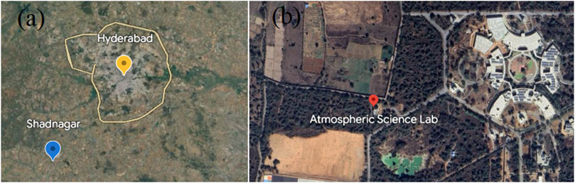
FIGURE 1. (A) Shadnagar, near the urban city Hyderabad; (B) the measurement location Atmosphere Science Laboratory, National Remote Sensing Centre, Shadnagar. Image source: Google Maps.

2.2 In situ measurements

The measurements of surface NO, NO₂, and O₃ were conducted from September 2014 to April 2017 at Shadnagar. In brief, an ozone analyzer (model 49i) works on the UV absorption technique with a wavelength of 254 nm (Thermo Fisher Scientific, 2011). The analyzer has a lower detection limit of 1.0 ppbv, a response time of 20 s, and a sample flow rate of 1–3 L per min. The NO_x analyzer (model 42i) works on the principle of the chemiluminescence technique (Thermo Fisher Scientific, 2015) with a detection limit of 0.4 ppbv, a response time of 40 s, and a sample flow rate of 0.6–0.8 L per min. To obtain accurate measurements, the analyzers were calibrated with zero and span limits regularly using a dynamic gas calibrator (model 146i) (Thermo Fisher Scientific, 2013) for the NO_x analyzer. The zero calibration for the ozone analyzer was performed using a dynamic gas calibrator, while span calibration was performed using its in-built ozone generator. More information about the calibration, accuracy, and full setup is given in the work of Kanchana et al. (2020). The gaseous species were measured with a resolution of 1 min during the whole study period. Any two consecutive time records with ±20 ppbv change in 1-min intervals were excluded. This procedure filtered out the spikes in concentration and erroneous data that occurred soon before and after the calibration. The gaseous data found between the 1st and 99th percentile were employed to eliminate the erroneous records from the measurements. The meteorological parameters, such as surface pressure, temperature and wind speed, and wind direction, were used at a 1-h time interval during the study period.

2.3 Chemical reanalysis data

We used Tropospheric Chemistry Reanalysis version 2 (Miyazaki et al., 2020) data products of surface NO, NO₂, and O₃ and meteorological parameters such as T, P, specific humidity (q), and horizontal wind components to study the mass balance of O₃ and its horizontal advection. All datasets have a spatial resolution of 1.125° latitude × 1.125° longitude, with a temporal resolution of 2 h. These data were obtained from the assimilation of multi-constituent measurements of multiple satellite sensors OMI, GOME-2, SCIAMACHY, MLS, TES, and MOPITT. The chemical species were optimized using an ensemble Kalman filter technique and evaluated by different independent observations. We validated the aforementioned chemical species and meteorological parameters with our direct in situ observation. The reanalysis data with 2 h of resolution were used to compare with in situ observations (Supplementary Figure S1). RH was not obtained directly; hence, it was calculated using specific humidity using the Clausius–Clapeyron equation, with inputs of surface temperature and pressure. The scatter plots between the in situ observations and chemical reanalysis data (O₃, NO, and NO₂), as well as the meteorological parameters at Shadnagar, show good correlations. The correlation values vary between 0.3 and 0.96 (see Supplementary Figure S1).

2.4 The steady state of ozone

The theoretical mass balance of ozone (Khalil, 2018) under a small volume at the point of observation for limited data can be written as

$\frac{\mathrm{d}\left(\left[{\mathrm{O}}_3\right]\right)}{\mathrm{d}\mathrm{t}}=\left[{\mathrm{P}}_{\mathrm{O}3}\right]+\frac{\left(\left[{\mathrm{O}}_3\right]\right)}{{\mathrm{\tau }}_{\mathrm{O}3}}+{\left[\mathrm{T}\right.}_{\mathrm{n}\mathrm{e}\mathrm{t}}{\mathrm{O}}_3],(3)$

$\left[{\mathrm{P}}_{\mathrm{n}\mathrm{e}\mathrm{t}}{\mathrm{O}}_3\right]={\mathrm{J}}_{\mathrm{N}\mathrm{O}2}\left(\left[\mathrm{N}{\mathrm{O}}_2\right]\right)-{\mathrm{k}}_4\left(\left.{\left[\mathrm{N}\mathrm{O}\left]\right[\mathrm{O}\right.}_3\right]\right),(4)$

where $\frac{\mathrm{d}\left(\left[{\mathrm{O}}_3\right]\right)}{\mathrm{d}\mathrm{t}}$, ${\mathrm{P}}_{\mathrm{n}\mathrm{e}\mathrm{t}}{\mathrm{O}}_3$, and ${\mathrm{T}}_{\mathrm{n}\mathrm{e}\mathrm{t}}{\mathrm{O}}_3$ in represent the rate of change of ozone, the net production, and the net transport of O₃ at the site, respectively. ${\mathrm{\tau }}_{\mathrm{O}3}$ is the lifetime of O₃ against the reaction with NO (R4). The production ${P_{\mathrm{O}3}=\mathrm{J}}_{\mathrm{N}\mathrm{O}2}\left(\left[\mathrm{N}{\mathrm{O}}_2\right]\right)$ and sink of ozone ${{\mathrm{S}}_{\mathrm{O}3}=\mathrm{k}}_4\left(\left.{\left[\mathrm{N}\mathrm{O}\right][\mathrm{O}}_3\right]\right)$ were calculated for each hour of the day. In the present study, | $\frac{\mathrm{d}\left(\left[{\mathrm{O}}_3\right]\right)}{\mathrm{d}\mathrm{t}}$ | < 10% of the term P_O3, S_O3, and T_netO₃ (Eq. 3) in the daytime, which validates the pseudo-steady-state criteria (Khalil, 2018). The mass balance equation provides the differentiation between the local net production and net transport of ozone. The difference between the actual ozone and the ozone under the photostationary state can be written as

$\left[\mathrm{\delta }{\mathrm{O}}_3\right]={\left[{\mathrm{O}}_3\right]}_{\mathrm{m}\mathrm{e}\mathrm{a}\mathrm{s}\mathrm{u}\mathrm{r}\mathrm{e}\mathrm{d}}-{\left[{\mathrm{O}}_3\right]}_{\mathrm{H}\mathrm{P}\mathrm{S}\mathrm{S}}={\mathrm{\tau }}_{\mathrm{O}3}\left[{\mathrm{T}}_{\mathrm{n}\mathrm{e}\mathrm{t}}{\mathrm{O}}_3\right].(5)$

The ozone in the photostationary state, when there is no transport and only NO, NO₂, O₃, and J_NO2 are present in the system, was calculated. The ozone concentration in the photostationary state was also calculated as $\mathrm{ɸ}{\left[{\mathrm{O}}_3\right]}_{\mathrm{m}\mathrm{e}\mathrm{a}\mathrm{s}\mathrm{u}\mathrm{r}\mathrm{e}\mathrm{d}}$.

We calculated the horizontal advection (ADV_O3) for the study location using the chemical reanalysis data to compare with the transport term.

${\mathrm{A}\mathrm{D}\mathrm{V}}_{\mathrm{O}3}=\nabla .\left(\mathbf{u}\left[{\mathrm{O}}_3\right]\right),(6)$

where u = (u_x, u_y) is the sum of the horizontal wind vectors representing the meridional and zonal winds, respectively.

Then, the horizontal component of advection (ppbv/h) was calculated using the central difference method along the grid boxes.

Since the observations of J_NO2 were not available at the site, we calculated J_NO2 values using the TUV (5.3.2) model for each hour of the day for the whole study period. The TUV model is a cloud-free radiative transfer model (Madronich, 1987). The daily satellite data were averaged monthly and provided to the model. The location parameters, latitude: 17.034°, longitude: 78.182°, and surface elevation: 550 m, including the measurement altitude of 10 m, were provided to the model, along with measurements from September 2014 to April 2017. The input parameters, such as monthly surface temperature and pressure data, were obtained using the Atmospheric Infrared Sounder (Olsen et al., 2013). The total column of ozone, nitrogen dioxide, sulfur dioxide, single scattering albedo, aerosol optical thickness at 342.5 nm, and angstrom exponent at 352 nm was obtained using the Ozone Monitoring Instrument (De Haan, 2009).

3 Results and discussion

3.1 Estimation of reaction constants of O₃ with NO

In the past, the rate constant for R4 was estimated in various studies, as tabulated in Table 1 (Birks et al., 1976; Lippmann et al., 1980; Michael et al., 1981; Ray and Watson, 1981; Borders and Birks, 1982; Moonen et al., 1998; Atkinson et al., 2004). To choose the preferred rate constant equation among the aforementioned studies, we applied the temperature observed at Shadnagar in each of the equations given in Table 1 to obtain their activation energy (E_a) and pre-exponential factor (A) of Eq. 1. The temperature at Shadnagar frequently reaches 27°C–30°C. For E_a and A, we estimated the log of the reaction rate constant (logk) referred to Eq. 1; furthermore, we plotted logk vs. 1/T (Figure 2A). From Eq. 1, one can infer that the slope of the line given in Figure 2A is equivalent to $-\frac{E_a}{R}$, where R is the gas constant. Figure 2B shows the frequency distribution of the hourly mean temperature at Shadnagar. The maximum frequency of temperature varies from 20°C to 32°C at the study site. Then, we took the average of the activation energy and pre-exponential constant. We replaced the activation energy and exponential constant in Eq. 1 to obtain the averaged rate constants. Using this rate constant of all six equations, the hourly ozone sink was obtained (Figure 2C). NO concentration was also plotted, as shown in Figure 2C (black line). We can observe that variations in the ozone sink and NO concentration are coherent. The averages of six (Figure 2C) pre-exponential factors and activation energy constant are averaged for all days for the study period (A = 3.62 × 10⁻¹² cm³/molecule-second and E_a/R = −1,537). Figure 2C shows that the maximum sink occurs between 08:00 and 10:00 h. This may be due to the emission of NO concentration.

TABLE 1

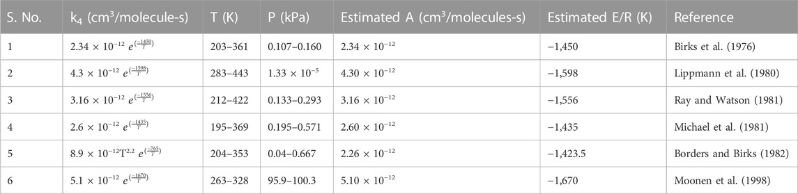
TABLE 1. Reaction rate constant for six different studies of the NO + O₃ reaction, including Arrhenius parameters, after applying Shadnagar temperature 281.76–315 K.

FIGURE 2

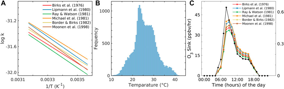
FIGURE 2. (A) Logk4 versus 1/T graph for different A and E_a values within the range of T, (B) frequency histogram of the reanalysis surface temperature (T) in the vertical axis; the x-axis shows the interval of temperature, and (C) sink of O₃ based on different rate constants and the average surface NO concentration in the y-axis and with time in the x-axis.

3.2 Net production of ozone

The hourly average of O₃ (Figure 3A), NO₂ (Figure 3B), and NO (Figure 3C) shows strong diurnal variation. The lowest O₃ mixing ratio (Figure 3A) was found in the morning which then started increasing and became maximum before evening (16:00 to 17:00 h). After reaching a maximum in the evening, it started decreasing until night. It became minimum between early morning 04:00 and 06:00 h. Fig. 3b shows that NO₂ starts decreasing from morning to evening. This may be the conversion of NO by photolysis and the reaction of peroxy radicals that might result in minimum NO₂ in the daytime (08:00 to 18:00 h). At night, NO₂ starts increasing from 18:00 h to morning at 10:00 h. This may be due to a lack of photolysis and anthropogenic emissions. Figure 3C shows that NO concentration is minimum in the daytime, which may be due to the photolysis of NO₂. During night, NO rapidly reacts with O₃ by the reaction (R4), which produces NO_x and quickly converts it to NO₂ (Seinfeld and Pandis, 2016), which might result in maximum NO₂ during nighttime. Figure 3D shows the ratio of NO to NO₂. It indicates that NO and NO₂ decrease in the daytime and become maximum at 07:00 to 10:00 h. The ratio of NO/NO₂ was found to be between 0.024 and 1.46 in the daytime, with an average value of 0.16. The low ratio indicates more NO₂ relative to NO at the site. The rate of change of ozone (Figure 3E) starts increasing from early morning to noon (07:00 to 15:00), and it becomes maximum between 09:00 and 11:00 h. The rate of change of ozone becomes negative after evening and reduces till the following early morning (16:00 to 05:00 h).

FIGURE 3

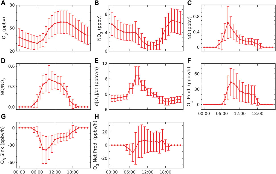
FIGURE 3. Diurnal variation of (A) O₃, (B) NO₂, (C) NO, and (D) NO/NO₂; (E) rate change of O₃; (F) production of O₃; (G) sink of O₃; and (H) net production of O₃. The error bar represents the ±1σ standard deviation from the mean at each hour.

Figure 3F shows the production of ozone (P_O3), which is due to the combination of atomic oxygen (produced after the photolysis of NO₂) and oxygen molecules occurring only in the daytime. Figure 3F also shows two peaks: first in the early morning (07:00 to 11:00 h) and then in the late evening (14:00 to 18:00 h). Both peaks may be associated due to the high emission of NO_x from fossil fuel combustion due to high vehicular traffic and industrial activities. After the peaks, ozone production decreases since there may be a decrease in the NO₂ (Figure 3B) concentration. Similar to our results, the peaks in the morning and late evening hours were also reported in other urban regions in India, e.g., Hyderabad (Yerramsetti et al., 2012; Venkanna et al., 2015), Chennai (Mohan and Saranya, 2019), and Mumbai (Raparthi et al., 2022), due to vehicular traffic and other anthropogenic activities. Another potential explanation is that throughout the night, NO combines with O₃ to generate NO₂, which leaves a large amount of NO₂ for photolysis in the morning (Zavala et al., 2020). However, NO₂ is removed in the atmospheric reaction with hydroxyl radicals and deposited on the surface.

Khalil et al. (2018) reported maximum production between 09:00 and noon. The maximum production was between 310 ppbv/h and 140 ppbv/h in May and December 2007, respectively, in all major urban cities in Saudi Arabia, while at our station, Shadnagar, the production rate varied between 2.6 ppbv/h and 211.1 ppbv/h at the same noontime. The sink of ozone (S_O3) due to the reaction of NO (R4) is estimated and shown in Figure 3G. However, there are other reasons for sinks such as dry deposition, which amounts to 20%–40% of ozone sink in the IGP region (Sharma et al., 2016). Therefore, NO and NO₂ were interconverted in the daytime by R3 and the photolysis of NO₂. In the nighttime, the photolysis of NO₂ does not occur (J_NO2 = 0) due to the absence of sunlight. NO rapidly reacted with O₃ to generate NO₂; therefore, high NO₂ and low NO concentration was observed at nighttime (Steinfeld et al., 2016). The sink was found to be maximum in the morning (07:00 to 11:00 h), after which it started decreasing till evening. Figure 3G shows the maximum sink at the same time whenever the NO concentration is maximum. The average sink of ozone (S_O3) was found to be 23.8 ± 75 ppbv/h during the study period. The high and low values of S_O3 occurred during the day and nighttime, respectively (Figure 3G). This is due to the high NO concentration in the daytime compared to nighttime (Figure 3B). The average sink was observed from morning (07:00 h) to noontime (11:00 h) at 25.9 ± 22.8 ppbv/h. At the same time, NO was found to be 0.5 ± 0.3 ppbv, while O₃ was observed at 34.8 ± 9.9 ppbv. NO concentration (Figure 3C) in the morning (07:00 to 10:00) provides high availability of NO for ozone sink.

Figure 3H shows that the net production of ozone decreased from early morning (05:00 to 09:00 h) and increased from late evening (09:00 to 18:00 h) throughout the study period. This is due to the sink starting to be dominant in the morning and, later, the production being dominant for the rest of the day. In the daytime, P_netO₃ can be explained based on the NO/NO₂ ratio as NO₂ and NO promote the production and dissociation of O₃, respectively (Annika, 2017). The ratio was higher in the daytime than at nighttime. The low ratio at night indicates that O₃ reacts with NO, resulting in a higher concentration of NO₂. In the morning traffic hours (07:00 to 10:00 h), the minimum value of P_netO₃ was lower due to the high NO/NO₂ ratio (Figure 4E). The higher ratio in the morning indicates that NO₂ is higher than NO, which might participate in the production of ozone. The ratio was observed at 0.08 ± 0.07 between 07:00 and 10:00 h, while it was 0.16 ± 0.07 between 09:00 and 18:00 h. The average net production of ozone was found to be 3.2 ± 19.5 ppbv/h during the study period, which suggests that ozone production dominated the sink at the site. Khalil et al.(2018) showed that the net production average value was 60–170 ppbv/h between 09:00 and 12:00 h at local noontime from 2000 to 2005 in some cities of temperate industrialized countries, such as Saudi Arabia. Similar values at an average of 28 ppbv/h to 120 ppbv/h were also reported in the peripheral and central cities of the Mexico City Metropolitan Area from 2015 to 2019 (Zavala et al., 2020). For the present Shadnagar location, the range of net production was from −79.77 ppbv/h to 170.60 ppbv/h from 09:00 to 12:00 h. The minimum values at Shadnagar were underestimated compared to the cities of Saudi Arabia (−249.77 ppb/h) and Mexico City Metropolitan Area (−107.77 ppbv/h). The maximum value was similar to that of cities of Saudi Arabia (0.6 ppbv/h) and overestimated in the Mexico City Metropolitan Area (50.6 ppb/h). The comparison of the mean values of different terms is provided in Supplementary Figure S2.

FIGURE 4

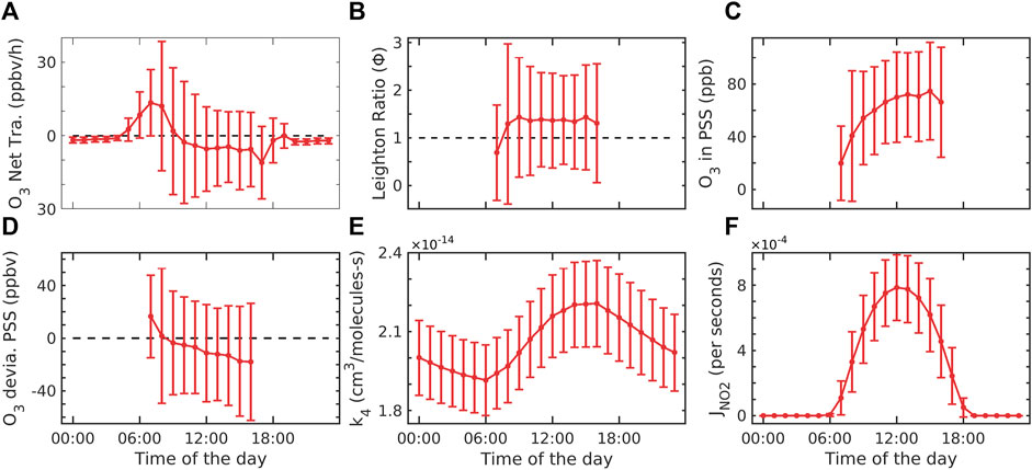
FIGURE 4. (A) Net transport of O₃, (B) Leighton ratio, (C) O₃ in PSS, (D) deviation of O₃ from the photostationary state, (E) reaction rate coefficient of R4, and (F) photolysis rate derived from the model. The error bar represents ±1σ standard deviation from the mean at each hour.

3.3 Tendency of ozone and net transport

Figure 4A shows the net transport of ozone at Shadnagar. The average net production is observed to be −1.6 ± 14.0 ppbv/h. It is 85.23% less than S_O3 and 87.13% less than P_O3 throughout the study period. The rate of change of ozone was found to be 2.7 ± 3.4 ppbv/h during daytime, and net production was 3.2 ± 19.5 ppbv/h during daytime (07:00 to 18:00 h). The maximum transport of ozone was found from 05:00 to 09:00 h. which is similar but negative to net production. Figure 4B shows the Leighton ratio. It can be used to separate local chemical production from transport (Khalil, 2018). Leighton ratio values were found to be 1.3 ± 1.2 in the daytime (07:00 to 18:00 h), while at nighttime, it was observed to be 0 due to no ozone production. Matsumoto et al. (2005) showed that the Leighton ratio is greater than 1 due to the involvement of peroxy radicals. There were no observations of peroxy radicals at our site. Hence, we cannot quantify the involvement of the peroxy radicals at our site during the study period. The Leighton ratio closer to 1 indicates that the steady-state assumption is valid and shows the involvement of species other than O₃, NO, NO₂, and J_NO2 in the system at Shadnagar. Figure 4C shows the mixing ratio in the photostationary state assumption. The ozone in the photostationary state was found to be 58.7 ± 39.3 ppbv, which was −16.32% of the real ozone. Figure 4D shows the photostationary state deviation from the real observed ozone. The actual concentration of ozone can be assumed to be the sum of ozone in a photostationary state and its deviation from the real environment, i.e., O₃ = O_3PSS+δO_3PSS. The deviation was negative throughout the study period in the daytime. Figure 4E shows the rate constant of reaction R4. The rate constant is directly dependent on the temperature variation, so a similar diurnal variation is found in the rate constant. The maximum values of k₄ were observed between 01:00 and 17:00 h throughout the study period. Figure 4F shows the photolysis of surface NO₂ calculated using the TUV model. J_NO2 was maximum at noontime from 12:00 to 14:00 h (4 × 10⁻³ s⁻¹ at the study site). A similar order of maximum values of J_NO2 (8.94 × 10⁻³ s⁻¹) was reported for Anantapur, Andhra Pradesh, a semi-urban location (Lingaswamy et al., 2017).

To concentrate on short-term oscillations or cycles, we eliminate the long-term trend from a time series by detrending the data. We calculated the detrend of in situ and reanalysis ozone by subtracting the linear trends from the time-series data. Figure 5A shows the detrend of daily average in situ and chemical reanalysis ozone. One can observe that the ozone detrends of in situ and chemical reanalysis ozone vary between −34.3 and 51.5 ppbv and −24.3 and 29.8 ppbv, respectively. The in situ and reanalysis ozone were found in similar phases and magnitude. The in situ ozone has a higher peak in the pre-monsoon season and a lower trough in the monsoon season. This indicates that in situ ozone is more sensitive to high ozone than reanalysis. Both data are comparable and showed seasonal cycles with higher values in the pre-monsoon season and lower values in the monsoon season.

FIGURE 5

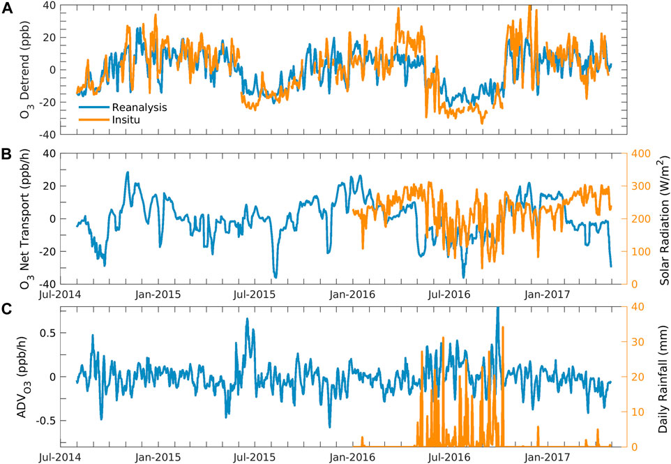
FIGURE 5. Daily daytime average of (A) detrend of chemical reanalysis and in situ ozone. (B) Net transport of ozone (or residual term) and solar radiation. (C) Horizontal advection of reanalysis surface ozone and daily rainfall at Shadnagar.

As we stated previously, the residual term, which is the difference between the net tendency of ozone and net production, can explain the net transport of ozone and the uncertainty remaining in the estimation of net ozone production (production + sink). Figure 5B shows the daytime daily average of the net transport of ozone and solar radiation from January 2016 to April 2017. Solar radiations affect the ozone production surface concentration (Kim and Lee, 2022). Net transport consists of horizontal and vertical transport. The net transport and solar radiation show seasonality and are consistent. The minimum trough found in the net transport and solar radiation was in the monsoon season, while the peak was in pre-monsoon season. The daily average of the net transport and detrend ozone simultaneously shows minimum and maximum values throughout the period. Figure 5C shows the time evolution of the horizontal advection, calculated using Eq. 6, and rainfall. The advection indicates how much ozone traveled horizontally, and rainfall suggests a cloudy sky, preventing ozone formation.

The average daily daytime horizontal advection for the surface layer was 0.01 ± 1 ppbv/h and varied between −1.01 ppbv/h and 1.7 ppbv/h in the study period. Ni et al. (2020) reported an average horizontal advection of 6.7 ppb/h for 24 August to 6 September using model studies in Hangzhou, China. There was a large variation in horizontal advection and net transport during monsoon, which might be due to the strong monsoon winds. The net transport of ozone was higher than the advection of ozone throughout the study period. It might be because the vertical transport can impact the net transport. Coherency can be observed in the detrend, net transport, and cloudy and rainfall conditions throughout the study period. The cloudy conditions or less-solar radiation conditions throughout monsoon resulted in maximum rainfall and minimum ozone production over the region. The surface ozone negatively correlates with cloud cover (Ghosh et al., 2011), and the absence of solar radiation decreased the photochemical production of ozone.

4 Conclusion

Here, we investigated the near-surface ozone balance in a suburban location, Shadnagar, India. The net production and net transport are derived from the photostationary state framework. Chemical reanalysis of NO, NO₂, and O_3, and TUV model-derived J_NO2 were utilized to estimate the source sink of O₃ at the study site. Overall, the following major conclusions can be drawn from this study:

• The reanalysis data (NO, NO₂, and O_3, and meteorological parameters such as T, P, and RH) were comparable with hourly in situ measurements.

• The reanalysis data were then used to study the mass balance of near-surface ozone following chemical kinematics. The average P_O3 and S_O3 were found to be 12.5 ± 20.5 ppbv/h and 10.9 ± 15.4 ppbv/h, respectively, throughout the study period. This indicates that the net production is dominant at the site throughout the study period. The net production was negative in the morning from 07:00 to 10:00 h and positive from 10:00 to 18:00 h. This is consistent with previous studies in India.

• The average daily daytime net production and net transport of ozone at Shadnagar were found to be 3.2 ppbv/h and 0.9 ppbv/h, respectively, indicating that the site is dominated by ozone production.

• The average horizontal advection of ozone was found to be 0.11 ± 1 ppbv/h and varied between 0.39 ppbv/h and 5.3 ppbv/h during the study period at the site. The average net transport of ozone is 0.9 ppbv/h. This indicates that the site is impacted by long-range transported ozone.

• The surface ozone variability is strongly controlled by production at Shadnagar and may be relevant for similar environments globally.

This study provides the near-surface ozone balance, but the direct observation of VOCs and J values is warranted to further explore ozone chemistry.

Data availability statement

The datasets presented in this article are not readily available because the surface data on O₃ and NO_x are part of the AT-CTM network collected under this project, which is under the ISRO Geosphere-Biosphere Program, and thus, the data will not be shared. The TES reanalysis data are freely available at “https://tes.jpl.nasa.gov/tes/chemical-reanalysis/.” Requests to access the datasets should be directed to the TES Chemical Reanalysis Product, https://tes.jpl.nasa.gov/tes/chemical-reanalysis/.

Author contributions

Conceptualisation by VKS, ALK, and RKN, formal analysis by VKS, writing of the original draft by VKS, VKS interpreted results with major inputs from SF, and all authors contributed to reviewing the manuscript.

Acknowledgments

The authors sincerely thank the Director, NRSC, for his kind support to carry out this work. This work was part of the Atmospheric Trace Gases—Chemistry, Transport, and Modelling (AT-CTM) of the ISRO Geosphere–Biosphere Program (IGBP). The authors thank Dr. M.V.R. Sesha Sai, Deputy Director, ECSA, for his constructive comments which helped improve the manuscript.

Conflict of interest

The authors declare that the research was conducted in the absence of any commercial or financial relationships that could be construed as a potential conflict of interest.

Publisher’s note

All claims expressed in this article are solely those of the authors and do not necessarily represent those of their affiliated organizations, or those of the publisher, the editors, and the reviewers. Any product that may be evaluated in this article, or claim that may be made by its manufacturer, is not guaranteed or endorsed by the publisher.

Supplementary material

The Supplementary Material for this article can be found online at: https://www.frontiersin.org/articles/10.3389/fenvs.2023.1178833/full#supplementary-material

References

Alghamdi, M. A., Al-Hunaiti, A., Arar, S., Khoder, M., Abdelmaksoud, A. S., Al-Jeelani, H., et al. (2019). A predictive model for steady state ozone concentration at an urban-coastal site. Int. J. Environ. Res. Public Health 16, 258. doi:10.3390/ijerph16020258

PubMed Abstract | CrossRef Full Text | Google Scholar

Atkinson, R., Baulch, D. L., Cox, R. A., Crowley, J. N., Hampson, R. F., Hynes, R. G., et al. (2004). Evaluated kinetic and photochemical data for atmospheric chemistry: Volume I - gas phase reactions of O_x, HO_x, NO_x and SO_x species. Atmos. Chem. Phys. 4, 1461–1738. doi:10.5194/acp-4-1461-2004

CrossRef Full Text | Google Scholar

Birks, J. W., Shoemakdr, B., Leck, T. J., and Hinton, D. M. (1976). Studies of reactions of importance in the stratosphere. I. Reaction of nitric oxide with ozone. J. Chem. Phys. 65, 5181–5185. doi:10.1063/1.433059

CrossRef Full Text | Google Scholar

Borders, R. A., and Birks, J. W. (1982). High-precision measurements of activation energies over small temperature intervals: Curvature in the Arrhenius plot for the reaction nitric oxide + ozone.fwdarw. Nitrogen dioxide + oxygen. J. Phys. Chem. 86, 3295–3302. doi:10.1021/J100214A007

CrossRef Full Text | Google Scholar

Chen, Y., Beig, G., Archer-Nicholls, S., Drysdale, W., Acton, W. J. F., Lowe, D., et al. (2021). Avoiding high ozone pollution in Delhi, India. Faraday Discuss. 226, 502–514. doi:10.1039/d0fd00079e

PubMed Abstract | CrossRef Full Text | Google Scholar

Conibear, L., Butt, E. W., Knote, C., Spracklen, D. V., and Arnold, S. R. (2018). Current and future disease burden from ambient ozone exposure in India. Geohealth 2, 334–355. doi:10.1029/2018GH000168

PubMed Abstract | CrossRef Full Text | Google Scholar

De Haan, Johan (2009). OMI/Aura ozone (O3) profile 1-orbit L2 swath 13x48km V003. Greenbelt, MA, USA: Goddard Earth Sciences Data and Information Services Center GES DISC. doi:10.5067/Aura/OMI/DATA2026

CrossRef Full Text | Google Scholar

Fadnavis, S., Dhomse, S., Ghude, S., Iyer, U., Buchunde, P., Sonbawne, S., et al. (2014). Ozone trends in the vertical structure of Upper Troposphere and Lower stratosphere over the Indian monsoon region. Int. J. Environ. Sci. Technol. 11, 529–542. doi:10.1007/s13762-013-0258-4

CrossRef Full Text | Google Scholar

Ghosh, D., Midya, S. K., Sarkar, U., and Mukherjee, T. (2011). Variability of surface ozone with cloud coverage over Kolkata, India. Available at: http://www.censusindia.

Google Scholar

Ghude, S. D., Jena, C., Chate, D. M., Beig, G., Pfister, G. G., Kumar, R., et al. (2014). Reductions in India’s crop yield due to ozone. Geophys Res. Lett. 41, 5685–5691. doi:10.1002/2014GL060930

CrossRef Full Text | Google Scholar

Haagen-Smit, A. J., and Fox, M. M. (1954). Photochemical ozone formation with hydrocarbons and automobile exhaust. Air Repair 4, 105–136. doi:10.1080/00966665.1954.10467649

CrossRef Full Text | Google Scholar

Han, S., Bian, H., Feng, Y., Liu, A., Li, X., Zeng, F., et al. (2011). Analysis of the relationship between O3, NO and NO2 in tianjin, China. Aerosol Air Qual. Res. 11, 128–139. doi:10.4209/aaqr.2010.07.0055

CrossRef Full Text | Google Scholar

Kanawade, V. P., Sebastian, M., and Dasari, P. (2022). Reduction in anthropogenic emissions suppressed new particle formation and growth: Insights from the COVID-19 lockdown. J. Geophys. Res. Atmos. 127. doi:10.1029/2021JD035392

CrossRef Full Text | Google Scholar

Kanchana, A. L., Sagar, V. K., Pathakoti, M., Mahalakshmi, D. V., Mallikarjun, K., and Gharai, B. (2020). Ozone variability: Influence by its precursors and meteorological parameters-an investigation. J. Atmos. Sol. Terr. Phys. 211, 105468. doi:10.1016/j.jastp.2020.105468

CrossRef Full Text | Google Scholar

Karl, T., Lamprecht, C., Graus, M., Cede, A., Tiefengraber, M., Vila-Guerau De Arellano, J., et al. (2023). High urban NO x triggers a substantial chemical downward flux of ozone. Available at: https://www.science.org.

Google Scholar

Khalil, M. A. K., Butenhoff, C. L., and Harrison, R. M. (2018). Ozone balances in urban Saudi Arabia. NPJ Clim. Atmos. Sci. 1, 27–29. doi:10.1038/s41612-018-0034-8

CrossRef Full Text | Google Scholar

Khalil, M. A. K. (2018). Steady states and transport processes in urban ozone balances. NPJ Clim. Atmos. Sci. 1, 22–27. doi:10.1038/s41612-018-0035-7

CrossRef Full Text | Google Scholar

Kim, M. J., and Lee, S. D. (2022). Potential effects of surface ozone on forests in Gangwon Province, South Korea, based on critical thresholds. Front. For. Glob. Change 5. doi:10.3389/ffgc.2022.996859

CrossRef Full Text | Google Scholar

Kunchala, R. K., Singh, B. B., Karumuri, R. K., Attada, R., Seelanki, V., and Kumar, K. N. (2022). Understanding the spatiotemporal variability and trends of surface ozone over India. Environ. Sci. Pollut. Res. 29, 6219–6236. doi:10.1007/s11356-021-16011-w

CrossRef Full Text | Google Scholar

Lefohn, A. S., Malley, C. S., Smith, L., Wells, B., Hazucha, M., Simon, H., et al. (2018). Tropospheric ozone assessment report: Global ozone metrics for climate change, human health, and crop/ecosystem research. Elementa 6, 1. doi:10.1525/elementa.279

PubMed Abstract | CrossRef Full Text | Google Scholar

Leighton, P. (1961). Photochemistry of air pollution. 1st ed. New York, NY, USA: Academic Press. Available at: https://www.elsevier.com/books/photochemistry-of-air-pollution/leighton/978-0-12-442250-6 (Accessed February 28, 2021).

Google Scholar

Lien, J., and Hung, H. M. (2021). The contribution of transport and chemical processes on coastal ozone and emission control strategies to reduce ozone. Heliyon 7, e08210. doi:10.1016/j.heliyon.2021.e08210

PubMed Abstract | CrossRef Full Text | Google Scholar

Lingaswamy, A. P., Arafath, S. M., Balakrishnaiah, G., Rama Gopal, K., Siva Kumar Reddy, N., Raja Obul Reddy, K., et al. (2017). Observations of trace gases, photolysis rate coefficients and model simulations over semi-arid region, India. Atmos. Environ. 158, 246–258. doi:10.1016/j.atmosenv.2017.03.048

CrossRef Full Text | Google Scholar

Lippmann, H. H., Jesser, B., and Schurath, U. (1980). The rate constant of NO + O3 → NO2 + O2 in the temperature range of 283–443 K. Int. J. Chem. Kinet. 12, 547–554. doi:10.1002/kin.550120805

CrossRef Full Text | Google Scholar

Madronich, S. (1987). Photodissociation in the atmosphere: 1. Actinic flux and the effects of ground reflections and clouds. J. Geophys Res. 92, 9740. doi:10.1029/JD092iD08p09740

CrossRef Full Text | Google Scholar

Mahajan, A. S., De Smedt, I., Biswas, M. S., Ghude, S., Fadnavis, S., Roy, C., et al. (2015). Inter-annual variations in satellite observations of nitrogen dioxide and formaldehyde over India. Atmos. Environ. 116, 194–201. doi:10.1016/j.atmosenv.2015.06.004

CrossRef Full Text | Google Scholar

Mao, Y. H., Yu, S., Shang, Y., Liao, H., and Li, N. (2022). Response of summer ozone to precursor emission controls in the Yangtze River Delta region. Front. Environ. Sci. 10. doi:10.3389/fenvs.2022.864897

CrossRef Full Text | Google Scholar

Matsumoto, J., Kosugi, N., Nishiyama, A., Isozaki, R., Sadanaga, Y., Kato, S., et al. (2006). Examination on photostationary state of NOx in the urban atmosphere in Japan. Atmos. Environ. 40, 3230–3239. doi:10.1016/j.atmosenv.2006.02.002

CrossRef Full Text | Google Scholar

Michael, J. V., Allen, J. E., and Brobst, W. D. (1981). Temperature dependence of the nitric oxide + ozone reaction rate from 195 to 369 K. J. Phys. Chem. 85, 4109–4117. doi:10.1021/j150626a032

CrossRef Full Text | Google Scholar

Miyazaki, K., Bowman, K., Sekiya, T., Eskes, H., Boersma, F., Worden, H., et al. (2020). Updated tropospheric chemistry reanalysis and emission estimates, TCR-2, for 2005-2018. Earth Syst. Sci. Data 12, 2223–2259. doi:10.5194/essd-12-2223-2020

CrossRef Full Text | Google Scholar

Mohan, S., and Saranya, P. (2019). Assessment of tropospheric ozone at an industrial site of Chennai megacity. J. Air Waste Manage Assoc. 69, 1079–1095. doi:10.1080/10962247.2019.1604451

PubMed Abstract | CrossRef Full Text | Google Scholar

Moonen, P. C., Cape, J. N., Storeton-West, R. L., and Mccolm, R. (1998). Measurement of the NO + O3 reaction rate at atmospheric pressure using realistic mixing ratios. J. Atmos. Chem. 29, 299–314. doi:10.1023/A:1005936016311

CrossRef Full Text | Google Scholar

Nelson, B. S., Stewart, G. J., Drysdale, W. S., Newland, M. J., Vaughan, A. R., Dunmore, R. E., et al. (2021). In situ ozone production is highly sensitive to volatile organic compounds in Delhi, India. Atmos. Chem. Phys. 21, 13609–13630. doi:10.5194/acp-21-13609-2021

CrossRef Full Text | Google Scholar

Ni, Z. Z., Luo, K., Gao, Y., Gao, X., Jiang, F., Huang, C., et al. (2020). Spatial–temporal variations and process analysis of O&amp;lt;sub&amp;gt;3&amp;lt;/sub&amp;gt; pollution in Hangzhou during the G20 summit. Atmos. Chem. Phys. 20, 5963–5976. doi:10.5194/acp-20-5963-2020

CrossRef Full Text | Google Scholar

Olsen, E. T., Manning, E., Blaisdell, J., Iredell, L., Gsfc, S., and Susskind, J. (2013). AIRS version 6 retrieval channel sets. 1–16. Available at: http://airs.jpl.nasa.gov/AskAirs.

Google Scholar

Payra, S., Gupta, P., Sarkar, A., Bhatla, R., and Verma, S. (2022). Changes in tropospheric ozone concentration over indo-gangetic plains: The role of meteorological parameters. Meteorology Atmos. Phys. 134, 96. doi:10.1007/s00703-022-00932-3

CrossRef Full Text | Google Scholar

Rahman, W., Beig, G., Barman, N., Hopke, P. K., and Hoque, R. R. (2021). Ambient ozone over mid-Brahmaputra Valley, India: effects of local emissions and atmospheric transport on the photostationary state. Environ. Monit. Assess. 193 (12). doi:10.1007/s10661-021-09572-3

CrossRef Full Text | Google Scholar

Raparthi, N., Debbarma, S., and Phuleria, H. C. (2022). Determination of heavy-duty vehicle emission factors from highway tunnel measurements in India: Laboratory vs. real-world study. Atmos. Pollut. Res. 13, 101581. doi:10.1016/j.apr.2022.101581

CrossRef Full Text | Google Scholar

Ray, G. W., and Watson, R. T. (1981). Kinetics of the reaction nitric oxide + ozone.fwdarw. nitrogen dioxide + oxygen from 212 to 422 K. J. Phys. Chem. 85, 1673–1676. doi:10.1021/J150612A015

CrossRef Full Text | Google Scholar

Seinfeld, J. H., and Pandis, S. N. (2016). Atmospheric chemistry and physics: from air pollution to climate change. 3rd Edn. Hoboken, NJ: John Wiley & Sons.

Sharma, S., Chatani, S., Mahtta, R., Goel, A., and Kumar, A. (2016). Sensitivity analysis of ground level ozone in India using WRF-CMAQ models. Atmos. Environ. 131, 29–40. doi:10.1016/j.atmosenv.2016.01.036

CrossRef Full Text | Google Scholar

Sicard, P., Agathokleous, E., Anenberg, S. C., De Marco, A., Paoletti, E., and Calatayud, V. (2023). Trends in urban air pollution over the last two decades: A global perspective. Sci. Total Environ. 858, 160064. doi:10.1016/j.scitotenv.2022.160064

PubMed Abstract | CrossRef Full Text | Google Scholar

Sreenivas, G., Mahesh, P., Subin, J., Lakshmi Kanchana, A., Venkata Narasimha Rao, P., and Kumar Dadhwal, V. (2016). Influence of meteorology and interrelationship with greenhouse gases (CO₂ and CH₄) at a suburban site of India. Atmospheric Chem. Phys. 16 (6), 3953–3967. doi:10.5194/acp-16-3953-2016

CrossRef Full Text | Google Scholar

Sreenivas, G. P. M., Mahalakshmi, D. V., Kanchana, A. L., Chandra, N., Patra, P. K., Raja, P., et al. (2022). Seasonal and annual variations of CO₂ and CH₄ at Shadnagar, a semi-urban site. Sci. Total Environ. 819, 153114. doi:10.1016/j.scitotenv.2022.153114

PubMed Abstract | CrossRef Full Text | Google Scholar

Steinfeld, J. I., Seinfeld, John H., and Spyros, N. P. (2016). Atmospheric chemistry and physics: From air pollution to climate change. 3rd, reprint ed., Hoboken, New Jersey, United States: Wiley. doi:10.1080/00139157.1999.10544295

CrossRef Full Text | Google Scholar

Tai, A. P. K., Sadiq, M., Pang, J. Y. S., Yung, D. H. Y., and Feng, Z. (2021). Impacts of surface ozone pollution on global crop yields: Comparing different ozone exposure metrics and incorporating Co-effects of CO2. Front. Sustain Food Syst. 5. doi:10.3389/fsufs.2021.534616

CrossRef Full Text | Google Scholar

Thera, B., Dominutti, P., Colomb, A., Michoud, V., Doussin, J. F., Beekmann, M., et al. (2022). O₃–NO_y photochemistry in boundary layer polluted plumes: Insights from the MEGAPOLI (paris), ChArMEx/SAFMED (North West Mediterranean) and DACCIWA (Southern West Africa) aircraft campaigns. Environ. Sci. Atmos. 2, 659–686. doi:10.1039/d1ea00093d

CrossRef Full Text | Google Scholar

Thermo Fisher Scientific, (2013). Model 146i instruction manual dynamic gas calibrator Part Number 102482-00 16Apr2013. Available at: www.thermo.com/WEEERoHS.

Google Scholar

Thermo Fisher Scientific, (2015). Model 42i instruction manual chemiluminescence NOx analyzer. Available at: www.thermo.com/WEEERoHS.

Google Scholar

Thermo Fisher Scientific, (2011). Model 49i instruction manual UV photometric O3 analyzer. Waltham, Massachusetts, United States: Thermo Fisher Scientifi.

Google Scholar

Trebs, I., Mayol-Bracero, O. L., Pauliquevis, T., Kuhn, U., Sander, R., Ganzeveld, L., et al. (2012). Impact of the Manaus urban plume on trace gas mixing ratios near the surface in the Amazon Basin: Implications for the NO-NO2-O 3 photostationary state and peroxy radical levels. J. Geophys. Res. Atmos. 117, 1–16. doi:10.1029/2011JD016386

CrossRef Full Text | Google Scholar

Venkanna, R., Nikhil, G. N., Siva Rao, T., Sinha, P. R., and Swamy, Y. V. (2015). Environmental monitoring of surface ozone and other trace gases over different time scales: Chemistry, transport and modeling. Int. J. Environ. Sci. Technol. 12, 1749–1758. doi:10.1007/s13762-014-0537-8

CrossRef Full Text | Google Scholar

Yerramsetti, V. S., Gauravarapu Navlur, N., Rapolu, V., Dhulipala, N. S. K. C., Sinha, P. R., Srinavasan, S., et al. (2013). Role of nitrogen oxides, black carbon, and meteorological parameters on the variation of surface ozone levels at a tropical urban site - Hyderabad, India. Clean. (Weinh) 41, 215–225. doi:10.1002/clen.201100635

CrossRef Full Text | Google Scholar

Zavala, M., Brune, W. H., Velasco, E., Retama, A., Cruz-Alavez, L. A., and Molina, L. T. (2020). Changes in ozone production and VOC reactivity in the atmosphere of the Mexico City Metropolitan Area. Atmos. Environ. 238, 117747. doi:10.1016/j.atmosenv.2020.117747

CrossRef Full Text | Google Scholar