Cloud-based data mapper (CDM): application for monitoring dry deposition of reactive nitrogen

Spatiotemporal monitoring of reactive nitrogen atmospheric deposition is essential for understanding its impact on sensitive ecosystems and quantifying cumulative effects. However, the sparsity of direct surface flux measurements combined with barriers in dissemination are major limiting factors in providing this information to decision makers and non-experts in a timely manner. This work addresses both aspects of this information gap by, 1) utilizing satellite-derived reactive nitrogen dry deposition data products that can be used by decision-makers to supplement the sparse direct surface flux measurements and 2) fill in measurement gaps. Therefore, we have developed a Reactive Nitrogen Flux Mapper (RNFM) component of the interactive Cloud-based Data Mapper (CDM) for providing easy access of satellite-derived reactive nitrogen (defined here as nitrogen dioxide (NO₂) and ammonia (NH₃)) dry deposition flux spatial maps/data to decision-makers/stakeholders over North America. The RNFM component of CDM has a Graphical User Interface (GUI) that allows users to specify the geographical regions and time periods for computing the average fluxes on the fly using an integrated cloud-based computing platform. The CDM architecture is flexible and can be upgraded in the future to take advantage of upstream satellite data directly on cloud platforms to provide results in near real-time.

Introduction

Atmospheric deposition is the process whereby gases and particles are removed from the atmosphere and transferred to the earth’s surface. The main modes of transfer are wet (through precipitation) and dry (through a diffusive transfer process at the surface) deposition (Vet et al., 2014). The deposition of reactive nitrogen (defined here as nitrogen dioxide (NO₂) and ammonia (NH₃)) represents an essential source of nutrients to plants and a limiting element for growth in many ecosystems. However, when reactive nitrogen is in excess it has harmful effects on terrestrial and aquatic ecosystems, including soil acidification (Galloway et al., 2003), eutrophication (Bergstrom and Jansson, 2006) and loss of biodiversity (Fenn et al., 2010; Simkin et al., 2016). Human activities (i.e., burning of fossil fuels and production of nitrogen-based fertilizers) have doubled the reactive nitrogen inputs to the environment with a proportional increase of atmospheric deposition on the earth’s surface since the start of the 20th century (Fowler et al., 2013).

In light of its importance, comprehensive monitoring of reactive nitrogen dry deposition flux is required to assess its ecological impacts. Yet, obtaining direct monitoring of dry deposition fluxes is limited as it is more challenging than wet deposition monitoring (Wolff et al., 2010), thus, at present, none of the measurement networks provide direct measurements of the former. The measurement networks for reactive nitrogen dry deposition are sparse in nature and lack the required spatial coverage. The existing measurement networks provide dry deposition flux estimates using the inferential method (which combines the concentration measurements with modelled dry deposition velocities; Wesely, 1989; Zhang et al., 2003), and can not be spatially interpolated like those of wet deposition due to the heterogeneity of dry deposition fields (Schwede and Lear, 2014).

On the contrary, satellite measurements of NO₂ and NH₃ with a daily global coverage offer a valuable data source to fill the measurement gaps and provide an opportunity to analyze the reactive nitrogen dry deposition fluxes spatially using the inferential method (Nowlan et al., 2014; Kharol et al., 2018). However, the processing of large datasets from satellites or models requires high-performance supercomputers that are not readily available to most users. Thus, providing easy access to this large data product to end-users (i.e., decision-makers and stakeholders) remains challenging. Presently, there is not any existing platform where decision-makers and stakeholders can easily access the spatiotemporal satellite-derived reactive nitrogen dry deposition flux information. The model or model-measurement fusion annual maps are available through regional/federal agencies (e.g., US EPA; https://www3.epa.gov/castnet/drydep.html), however, they do not provide the flexibility to users for custom selection (i.e., geographical region and time period) and require >2 years to be produced. In recent years, commercial cloud-computing platforms are becoming popular in the scientific community and have become a valuable alternative for large data processing and complex earth science model runs with its massive computing power and data storage capability. For example, recently, Amazon Web Services (AWS) cloud-computing platforms have successfully been used to run the Goddard Earth Observing System (GEOS)-Chem global 3-D chemical transport model (Zhuang et al., 2020) at 50-km horizontal resolution.

In an attempt to fill this gap we have utilized a cloud-computing platform for space-based earth observations. Here, we describe the newly developed Reactive Nitrogen Flux Mapper (RNFM) component of the interactive Cloud-based Data Mapper (CDM) with user-friendly features (such as custom selection of geographical region and date range through the Graphical User Interface (GUI)) that provides easy access of satellite-derived reactive nitrogen dry deposition fluxes to end-users.

Reactive nitrogen flux Mapper

The overall schematic of the processing flow describing the RNFM is provided in Figure 1. The upstream preprocessed daily reactive nitrogen dry deposition fluxes are currently computed offline (as described in Appendix A, B) and uploaded to a cloud computing platform together with NH₃ and NO₂ dry deposition velocities and concentrations information. Statistical information and pre-rendered files (i.e daily, monthly, yearly) are then processed, and hosted on the cloud virtual machine (VM) using a Web Map Service (WMS) server. Gridded averages of concentrations, dry deposition velocities and fluxes (i.e., monthly, annual) are calculated using the equations described in Appendix C on the cloud virtual machine (VM). Using the RNFM GUI, users can search for pre-rendered data and retrieve datasets hosted on the VM to be displayed using the WMS on the interactive map as described in Figure 1. The WMS server on the cloud in tandem with our GUI will dynamically load and display the pre-rendered datasets on an interactive map. This allows users to zoom/scroll along the interactive map while the dataset is dynamically loaded from the WMS. In addition to that, the RNFM GUI provides custom selection (i.e., date range and geographical region) flexibility to users where they can select any date range during 2018-to-2020 and geographical coordinates over North America to calculate the averages on the fly. This process is shown in Figure 4. Even though the RNFM GUI provides the flexibility to define a user-specified date range, we recommend using at least a month-long date range selection as this will significantly increase the flux signal compared to the noise in the measurements.

FIGURE 1

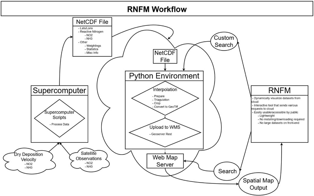
FIGURE 1. Schematic of the process flow of the Reactive Nitrogen Flux Mapper.

There are two processing streams used for generating datasets for the user through the WMS server on the cloud. The first is the aforementioned pre-rendering of data into standard time-series (i.e., daily and monthly files) where the intensive workload is already done allowing for very quick viewing and loading of the datasets, and the second being more custom dynamic searches for subsets of data that have not already been rendered (pre-processed). An example of the custom dynamic process flow would be good if the client makes a request to the cloud using the RNFM custom selection that has not already been pre-processed (i.e., the weighted average of data from 15 March 2018 to 31 July 2018). In this case, the algorithms on the cloud are used to process and render the requested data in real time that will then be displayed on the user’s local machine when completed. Since the rendering needs to be done, the trade-off for this is that it takes some time to complete before being displayed on the client’s local machine. This means that for both workflows all intensive work is already pre-done on the cloud or will be done on the cloud. This provides a user-friendly way for users to quickly view and analyze various complex datasets with minimal system requirements and performance. The RNFM application can be accessed through https://atmoanalytics.com/rnfm.html.

Figure 2 shows the study area domain map of RNFM where the points represent the latitude/longitude coordinates for which samples were attempted on each day. This region is defined by the GEM regional model output, but can be expanded depending on the availability of model outputs as the satellite observations themselves are global. Fill values (i.e., Nan) are assigned if good quality satellite observations for a specific region are not available (e.g., due to cloud cover). While the majority of data processing is currently performed offline on supercomputers, there are some extra steps needed to format this preprocessed data in such a way that it can be served via the WMS server hosted on the cloud to the end-users.

FIGURE 2

FIGURE 2. Domain boundaries of RNFM.

Since satellite observations are typically not on a regular grid, a Triangular Interpolation Network technique is used to format the satellite data into a gridded raster format that also allows datasets to be served to the end-users via the WMS from the cloud. Then these gridded raster files are clipped by the border file (as shown above in Figure 2), which is generated using a convex hull algorithm on all sampled point data. Once these steps are complete, the raster files are uploaded to the WMS server on the cloud and accessed from the RNFM. These algorithms are already performed for standard time-series, or are done on-the-fly from custom user searches on the cloud as stated earlier.

In order to visualize the datasets (which are residing on the cloud platform) on a user’s local machine, the user will first need to specify the required inputs using the “Range” and “Dataset” tabs in the search parameters as shown in Figure 3. Here the daily, monthly, and yearly search parameters will display pre-rendered datasets from the specified day/month/year, whereas the custom search parameter will display datasets that will be dynamically processed on the cloud for the specified date range. After this, the user can specify the dataset (one selection at a time) to view the surface concentration, dry deposition velocity, and dry deposition flux for nitrogen dioxide and ammonia. Once these parameters are specified, the user can search for the specified dataset, with the option of providing a user-specified name for the layer that will be displayed on the map. If the layer name is not defined by the user, then a name will be generated automatically for the layer based on their search parameters. Optional parameters include displaying the layer with a custom color palette and searching for data within a specified geographical region. These optional parameters can also be changed later on for that layer as the user sees fit.

FIGURE 3

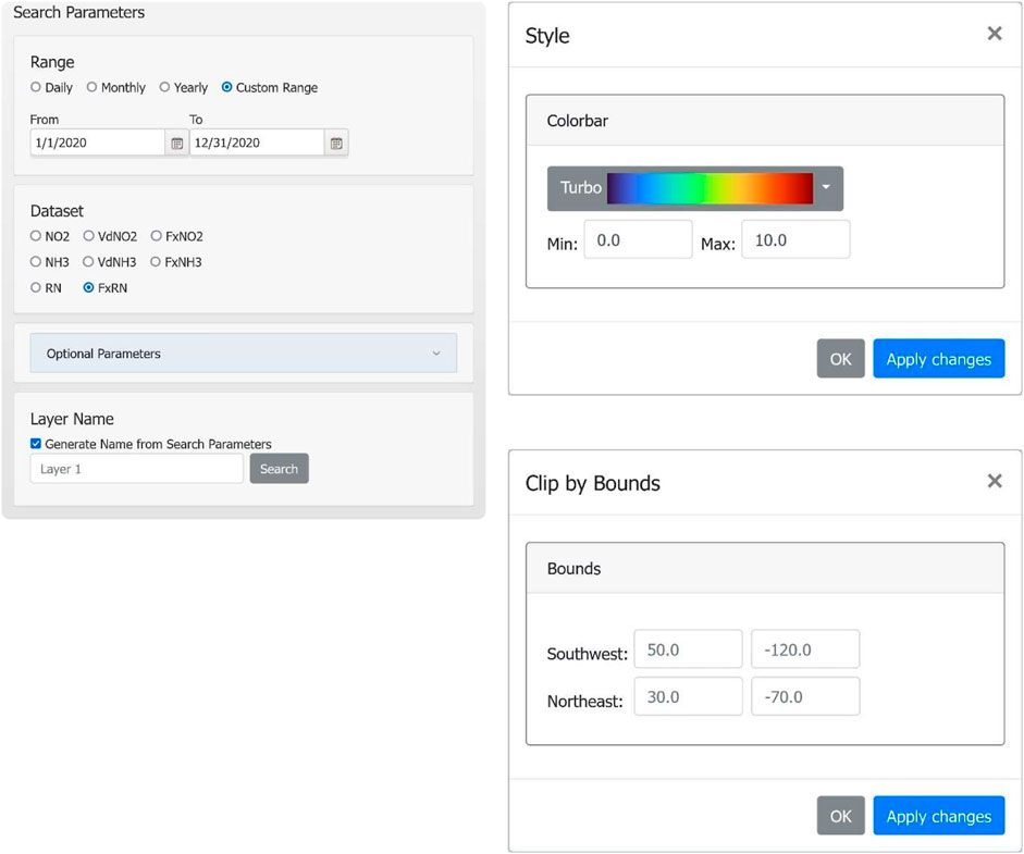
FIGURE 3. Popup that allows the user to define the search parameters and stylize the specified searched layer or clip the specified searched layer by Southwest/Northeast Latitudes/Longitudes bounds that were right-clicked from the layer tree.

After searching for a specified dataset through search parameters (an example shown in Figure 3), the layer will be added to the layer tree with user-specified or automatically generated layer name as shown in Figure 4. The layer tree is a powerful tool that allows users to work with multiple datasets on a single map. The layer tree also allows the users to select their choice of basemap, topographical layer, state/province boundaries to be displayed together with the selected datasets map. In addition to that, the interactive layer tree allows users to add/remove layers to the map by checking/unchecking their corresponding check box. Checked layers are then displayed in order from the bottom to top where the bottom layers of the layer tree overlay the layers above it on the map. The base maps at the top of the layer tree are rendered first on the map and are overlaid by the following checked layers. Users can also drag and drop layers on the layer tree to new positions, which will affect the order they are displayed on the map.

FIGURE 4

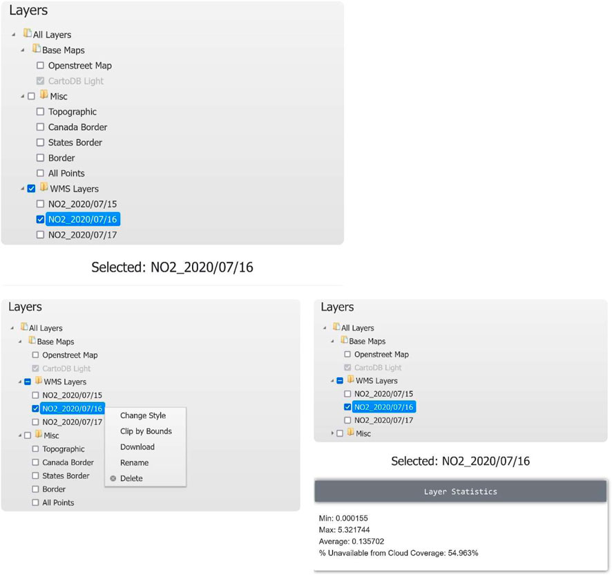
FIGURE 4. The layer tree of RNFM with different functions that can be performed on individual layers by right-clicking or selecting one.

Since layers have their own unique features, various functions can be performed on individual layers. The user has multiple options to customize the layer as they see fit including changing the layer’s style, opacity and clippings by selecting (or “right-clicking”) a layer in the layer tree. The general statistics for that given layer (i.e., min, max, average, percentage of points affected by cloud coverage) will be displayed by selecting a layer (as shown in a blue highlight when selected), and provide the flexibility to user’s to modify the selected layer through multiple tools. These tools are selectable on the top left corner of the interactive map and allow the user to clip the layer by drawing rectangles or their own custom polygons as shown in Figure 5, and also provide an option to change the opacity of the layer using the opacity function.

FIGURE 5

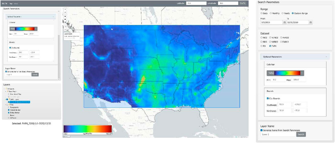
FIGURE 5. Example of clipped 3 year mean reactive nitrogen (Nr) dry deposition flux data for the period of 1/1/2018–12/31/2020 from Southwest to Northeast bounding box.

Figure 6 shows the 3-year mean (2018–2020) reactive nitrogen dry deposition flux map generated by RNFM in real time using the custom range selection and preprocessed data files uploaded on the cloud. Similar to reactive nitrogen dry deposition flux map, users can generate the average map of any datasets (e.g., reactive nitrogen concentration, NH₃ and NO₂ concentration etc.) defined in search parameters under the datasets option for their choice of custom date range and geographical region. The selection of a custom date range is one of the key features of RNFM which provides more flexibility to users to select any time-period to generate the average maps instead of pre-defined averages within the RNFM domain region.

FIGURE 6

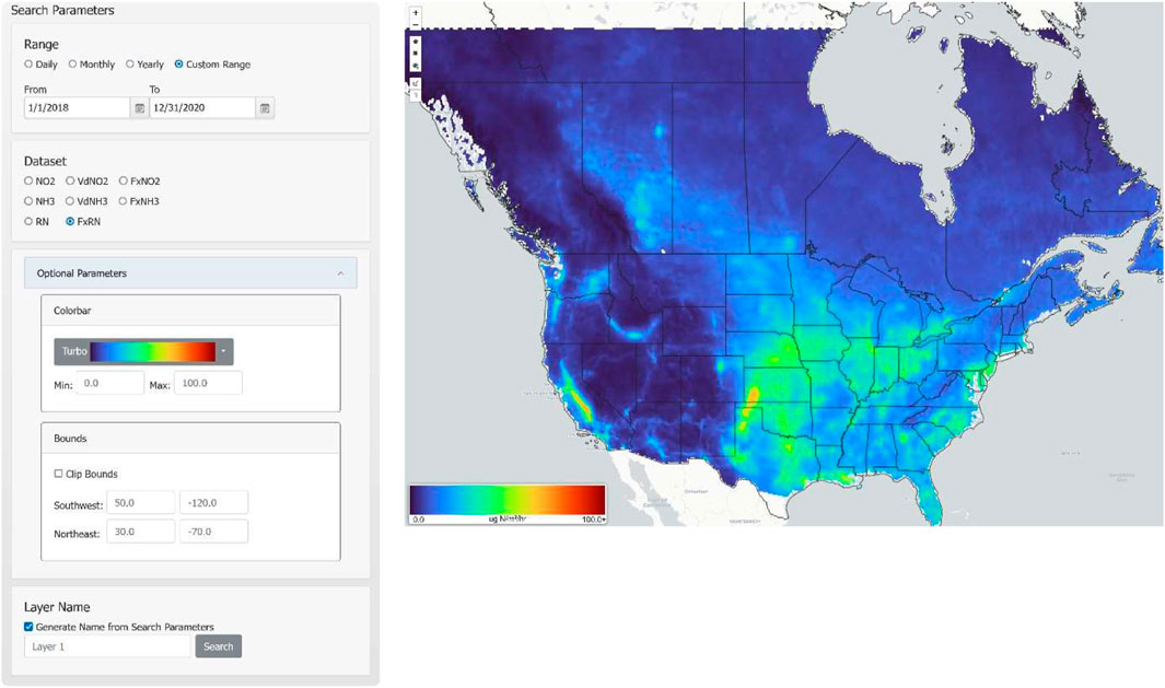
FIGURE 6. An example of RNFM with the inputted search parameters and the resultant map of 3-year average reactive nitrogen dry deposition flux map for 1/1/2018 to 12/31/2020 over North America.

Application

To illustrate RNFM’s ability to readily provide the reactive nitrogen flux information for interpretation we have applied it to example case studies. An overall example is provided in Figure 7 showing 3-year average maps of NH₃, NO₂ and reactive nitrogen (Nr (NH₃+NO₂)) dry deposition fluxes across North America that were generated using the RNFM’s custom range on-the-fly options. The individual spatial distribution maps of NH₃ and NO₂ dry deposition fluxes in Figure 7 shows that the elevated NH₃ dry deposition generally coincides with the agricultural regions, whereas the NO₂ dry deposition hotspots are mainly located over the cities and industrial regions across North America (Kharol et al., 2018). The combined spatial map of reactive nitrogen dry deposition flux provides cumulative information of the reactive nitrogen deposition from both atmospheric species.

FIGURE 7

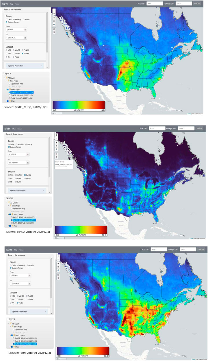
FIGURE 7. Three-year average dry deposition flux map of NH₃, NO₂, and Nr (NH₃+NO₂) for 1/1/2018 to 12/31/2020 over North America.

Another example application is the use of RNFM to investigate the changes in the reactive nitrogen dry deposition fluxes by season. Figure 8 shows the seasonal maps of reactive nitrogen dry deposition fluxes for winter (December-January-February), spring (March-April-May), summer (June-July-August) and fall (September-October-November) over North America for the period of December 2019 to November 2020. The NH₃ and NO₂ emissions and lifetime (McLinden et al., 2014; Shephard et al., 2020) as well as their dry deposition velocities (Zhang et al., 2003) vary by season and affect the ambient concentrations and its deposition. It is evident from Figure 8 that the reactive nitrogen deposition from NH₃ is greater during the growing season (i.e., spring and summer) over the agricultural regions (Shephard et al., 2020), whereas deposition from NO₂ is greater during fall and winter seasons in urban/industrial regions (Nowlan et al., 2014; Kharol et al., 2018).

FIGURE 8

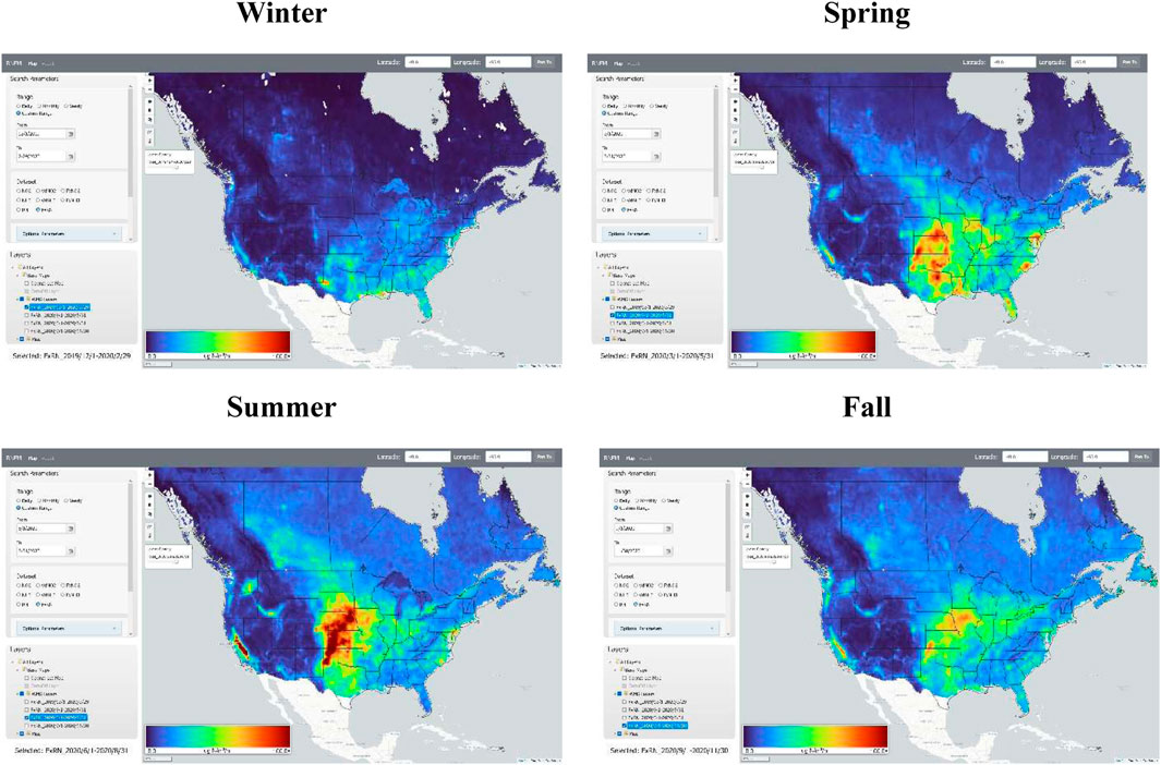
FIGURE 8. Seasonal maps of reactive nitrogen dry deposition fluxes for winter (December-January-February), spring (March-April-May), summer (June-July-August) and fall (September-October-November) over North America for the period of December 2019 to November 2020.

As previously noted, the RNFM also provides an opportunity for users to zoom into a region of interest and visualize/analyze the reactive nitrogen dry deposition in greater detail for that area.

To demonstrate this, here we have clipped the 3-year average of NH₃, NO₂ and Nr dry deposition fluxes over the province of Alberta, Canada as shown in Figure 9. The province of Alberta, Canada is a good example as it has separated source regions of NH₃ and NO₂. As seen in Figure 9 the NO₂ dry deposition hotspots are mostly located near/over the Athabasca oil sands region (Latitude: 57.02 N, Longitude: 111.65 W), urban and industrial regions. Also shown in the figure are the large NH₃ hotspots in and around Lethbridge (Latitude: 49.69 N, Longitude: 112.84 W), which has many concentrated animal feeding operations (CAFOs)) and the main agricultural regions of the province. These example applications demonstrate how easily RNFM can make new research results available to make informed decisions on mitigation strategies for environmental protection in a timely manner.

FIGURE 9

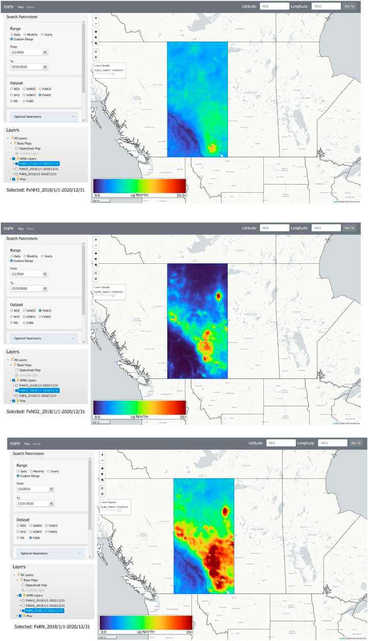
FIGURE 9. Average dry deposition flux map of NH₃, NO₂, and Nr (NH₃+NO₂) for 3-year period (1/1/2018 to 12/31/2020) over Alberta, Canada.

Summary

The RNFM component of interactive CDM allows users to obtain easy access to the new satellite-derived dry deposition of reactive nitrogen from NO₂ and NH₃ using a user-friendly GUI. The RNFM component provides researchers, stakeholders, and other interested parties with access to new scientific research information on the cumulative effects of reactive nitrogen in land and water ecosystems that can lead to soil acidification, biodiversity loss, and eutrophication (e.g., algal blooms). The CDM is a powerful cloud-based platform application that generates and displays large satellite-derived datasets alleviating numerous hurdles that would otherwise make it much more difficult, time consuming, and resource demanding (storage and computational burden) for users to work with in a meaningful way. The RNFM component of CDM helps overcome the scarcity of ground-based reactive nitrogen dry deposition flux measurements by providing additional new satellite-based information that decision-makers can use to make more informed and timely decisions on mitigation strategies for environmental protection. This CDM architecture can also be enhanced in the future to take advantage of upstream near real time observations directly available on cloud computing platforms.

Data availability statement

The raw data supporting the conclusion of this article will be made available by the authors, without undue reservation.

Author contributions

SK developed the reactive nitrogen dry deposition results. CP developed an interactive cloud-based Reactive Nitrogen Flux Mapper (RNFM). MS developed the CrIS CFPR Level 3 gridded ammonia product. CM and DG developed the TROPOMI NO2 Level 3 gridded product. All authors contributed to the article and approved the submitted version.

Acknowledgments

We would like to acknowledge the Labs Canada and Environment and Climate Change Canada for the funding support.

Conflict of interest

Author SK was employed by the company AtmoAnalytics Inc.

The remaining authors declare that the research was conducted in the absence of any commercial or financial relationships that could be construed as a potential conflict of interest.

Publisher’s note

All claims expressed in this article are solely those of the authors and do not necessarily represent those of their affiliated organizations, or those of the publisher, the editors and the reviewers. Any product that may be evaluated in this article, or claim that may be made by its manufacturer, is not guaranteed or endorsed by the publisher.

References

Bergstrom, A.-K., and Jansson, M. (2006). Atmospheric nitrogen deposition has caused nitrogen enrichment and eutrophication of lakes in the northern hemisphere. Glob. Change Biol. 12, 635–643. doi:10.1111/j.1365-2486.2006.01129.x

CrossRef Full Text | Google Scholar

Bey, I., Jacob, D. J., Yantosca, R. M., Logan, J. A., Field, B. D., Fiore, A. M., et al. (2001). Global modeling of tropospheric chemistry with assimilated meteorology: Model description and evaluation. J. Geophys. Res. 106 (D19), 23,073–23,095. doi:10.1029/2001jd000807

CrossRef Full Text | Google Scholar

Fenn, M. E., Allen, E. B., Weiss, S. B., Jovan, S., Geiser, L. H., Tonnesen, G. S., et al. (2010). Nitrogen critical loads and management alternatives for N-impacted ecosystems in California. J. Environ. Manag. 91, 2404–2423. doi:10.1016/j.jenvman.2010.07.034

PubMed Abstract | CrossRef Full Text | Google Scholar

Fowler, D., Coyle, M., Skiba, U., Sutton, M. A., Cape, N., Reis, S., et al. (2013). The global nitrogen cycle in the twenty-first century. Phil. Trans. R. Soc. B 368, 20130164. doi:10.1098/rstb.2013.0164

PubMed Abstract | CrossRef Full Text | Google Scholar

Galloway, J. N., Aber, J. D., Erisman, J. W., Seitzinger, S. P., Howarth, R. W., Cowling, E. B., et al. (2003). The nitrogen cascade. Bioscience 53, 341–356. doi:10.1641/0006-3568(2003)053[0341:tnc]2.0.co;2

CrossRef Full Text | Google Scholar

Griffin, D., Zhao, X., McLinden, C. A., Boersma, F., Bourassa, A., Dammers, E., et al. (2019). High-resolution mapping of nitrogen dioxide with TROPOMI: First results and validation over the Canadian oil sands. Geophys. Res. Lett. 46, 1049–1060. doi:10.1029/2018GL081095

PubMed Abstract | CrossRef Full Text | Google Scholar

Kharol, S. K., Shephard, M. W., McLinden, C. A., Zhang, L., Sioris, C. E., O’Brien, J. M., et al. (2018). Dry deposition of reactive nitrogen from satellite observations of ammonia and nitrogen dioxide over North America. Geophys. Res. Lett. 45, 1157–1166. doi:10.1002/2017GL075832

CrossRef Full Text | Google Scholar

McLinden, C. A., Fioletov, V., Boersma, K. F., Kharol, S. K., Krotkov, N., Lamsal, L., et al. (2014). Improved satellite retrievals of NO2 and SO2 over the Canadian oil sands and comparisons with surface measurements. Atmos. Chem. Phys. 14, 3637–3656. doi:10.5194/acp-14-3637-2014

CrossRef Full Text | Google Scholar

Moran, M. D., Ménard, S., Talbot, D., Huang, P., Makar, P. A., Gong, W., et al. (2010). “Particulate-matter forecasting with GEM-MACH15, A new Canadian air-quality forecast model,” in Air pollution modelling and its application XX (Dordrecht, Netherlands: Springer).

Google Scholar

Nowlan, C. R., Martin, R. V., Philip, S., Lamsal, L. N., Krotkov, N. A., Marais, E. A., et al. (2014). Global dry deposition of nitrogen dioxide and sulfur dioxide inferred from space-based measurements. Glob. Biogeochem. Cycles 28, 1025–1043. doi:10.1002/2014GB004805

CrossRef Full Text | Google Scholar

Pendlebury, D., Gravel, S., Moran, M. D., and Lupu, A. (2018). Impact of chemical lateral boundary conditions in a regional air quality forecast model on surface ozone predictions during stratospheric intrusions. Atmos. Environ. 174, 148–170. doi:10.1016/j.atmosenv.2017.10.052

CrossRef Full Text | Google Scholar

Schwede, D. B., and Lear, G. G. (2014). A novel hybrid approach for estimating total deposition in the United States. Atmos. Environ. 92, 207–220. doi:10.1016/j.atmosenv.2014.04.008

CrossRef Full Text | Google Scholar

Shephard, M. W., and Cady-Pereira, K. E. (2015). Cross-track infrared sounder (CrIS) satellite observations of tropospheric ammonia. Atmos. Meas. Tech. 8, 1323–1336. doi:10.5194/amt-8-1323-2015

CrossRef Full Text | Google Scholar

Shephard, M. W., Dammers, E., Cady-Pereira, K. E., Kharol, S. K., Thompson, J., Gainariu-Matz, Y., et al. (2020). Ammonia measurements from space with the cross-track infrared sounder: Characteristics and applications. Atmos. Chem. Phys. 20, 2277–2302. doi:10.5194/acp-20-2277-2020

CrossRef Full Text | Google Scholar

Simkin, S. M., Allen, E. B., Bowman, W. D., Clark, C. M., Belnap, J., Brooks, M. L., et al. (2016). Conditional vulnerability of plant diversity to atmospheric nitrogen deposition across the United States. Proc. Natl. Acad. Sci. 113 (15), 4086–4091. doi:10.1073/pnas.1515241113

PubMed Abstract | CrossRef Full Text | Google Scholar

Vet, R., Artz, R. S., Carou, S., Shaw, M., Ro, C. U., Aas, W., et al. (2014). A global assessment of precipitation chemistry and deposition of sulfur, nitrogen, sea salt, base cations, organic acids, acidity and pH, and phosphorus. Atmos. Environ. 93, 1–2. doi:10.1016/j.atmosenv.2013.11.013

CrossRef Full Text | Google Scholar

Wesely, M. (1989). Parameterization of surface resistances to gaseous dry deposition in regional-scale numerical models. Atmos. Environ. 23 (6), 1293–1304.

CrossRef Full Text | Google Scholar

White, E., Shephard, M. W., Cady-Pereira, K. E., Kharol, S. K., Ford, S., Dammers, E., et al. (2023). Accounting for non-detects: Application to satellite ammonia observations. Remote Sens. 15 (10), 2610. doi:10.3390/rs15102610

CrossRef Full Text | Google Scholar

Wolff, V., Trebs, I., Ammann, C., and Meixner, F. X. (2010). Aerodynamic gradient measurements of the NH3-HNO3-NH4NO3 triad using a wet chemical instrument: An analysis of precision requirements and flux errors. Atmos. Meas. Tech. 3, 187–208. doi:10.5194/amt-3-187-2010

CrossRef Full Text | Google Scholar

Zhang, L., Brook, J. R., and Vet, R. (2003). A revised parameterization for gaseous dry deposition in air-quality models. Atmos.Chem. Phys. 3, 2067–2082. doi:10.5194/acp-3-2067-2003

CrossRef Full Text | Google Scholar

Zhang, J., Moran, M. D., Zheng, Q., Makar, P. A., Baratzadeh, P., Marson, G., et al. (2018). Emissions preparation and analysis for multiscale air quality modeling over the Athabasca Oil Sands Region of Alberta, Canada. Atmos. Chem. Phys. 18 (14), 10,459–10,481. doi:10.5194/acp-18-10459-2018

CrossRef Full Text | Google Scholar

Zhuang, J., Jacob, D. J., Lin, H., Lundgren, E. W., Yantosca, R. M., Gaya, J. F., et al. (2020). Enabling high-performance cloud computing for Earth science modeling on over a thousand cores: Application to the GEOS-Chem atmospheric chemistry model. J. Adv. Model. Earth Syst. 12, e2020MS002064. doi:10.1029/2020MS002064

CrossRef Full Text | Google Scholar

Appendix A:

Datasets

Ammonia (NH₃)

We use the NASA/NOAA SNPP Cross-Track Infrared Sounder Satellite (CrIS, v1.6.3) retrieved level-3 gridded surface NH₃ concentrations obtained from the CrIS Fast Physical Retrieval algorithm (CFPR), which is described in detail by Shephard and Cady-Pereira (2015), and with updates in Shephard et al. (2020) and White et al. (2023) for the period of 2018–2020 over North America. CrIS is an infrared nadir pointing instrument in a sun-synchronous orbit (824 km) with a mean local daytime overpass time of 13:30, and a mean local nighttime overpass time of 1:30 in the descending node. Here, we only used daytime (i.e., 13:30 LST) satellite observations and filtered the data for clouds.

Nitrogen dioxide (NO₂)

Unlike NH3, the main retrieved parameter of NO₂ from the Sentinel-5P (S5P) TROPOspheric Monitoring Instrument (TROPOMI) version 2 (S5P-PAL) data is a total column values that then must be converted to a surface concentration values in a two-step process that utilizes output from the Environment and Climate Change Canada (ECCC) Global Environmental Multi-scale - Modelling Air quality and Chemistry (GEM-MACH) regional air quality model. First, the tropospheric vertical column densities (VCDs) are improved for North American monitoring using the approach described in Griffin et al. (2019), and then the VCDs are converted to surface concentrations following the approach described in McLinden et al. (2014) by scaling the satellite derived VCDs by the ratio of the model surface concentration to model VCD:

$C=V_{t\_satellite}\times {\left(\frac{C}{V_t}\right)}_{model}(1)$

Where $C$ is the surface concentration (ppb), and $V_t$ is the tropospheric VCD. For the model profile and surface concentrations, the GEM-MACH operational model is utilized (Moran et al., 2010; Pendlebury et al., 2018) with a 10 × 10 km² grid cell size for the North American domain. The operational forecast makes use of 2013 emissions information (Zhang et al., 2018). For the conversion we select the daily model output with the closest coincidence to the observation. Since the operational GEM-MACH model is missing sources in the free troposphere, such as lightning and aircraft, a monthly mean GEOS-Chem free tropospheric VCDs (Bey et al., 2001) are added to the GEM-MACH VCDs. These correspond to adjustments of ∼0.3-1e15 molec/cm².

TROPOMI is a nadir-viewing spectrometer on board the S5P satellite, launched on 13 October 2017. TROPOMI is in a sun-synchronous orbit with an overpass time of 13:30 LST and provides near-daily global coverage of NO₂ with a ground spatial resolution of 3.5 × 5.5 km². More details about TROPOMI are described in Griffin et al. (2019). Here, we only use the TROPOMI observations with “quality assurance value” (qa_value) ≥ 0.75 (the recommended pixel filter, https://sentinel.esa.int/documents/247904/3541451/Sentinel-5P-Nitrogen-Dioxide-Level-2-Product-Readme-File), which remove the less accurate observations (i.e., cloud-covered observations, snow/ice covered observations, errors, and problematic retrievals).

Appendix B:

DRY deposition flux calculation

The daily reactive nitrogen dry deposition fluxes are computed using an inferential method, which combines modeled dry deposition velocities according to the resistance analogy (Wesely, 1989; Zhang et al., 2003) and satellite-derived near-surface observations of NH₃ and NO₂ over North America between 2018–2020. The deposition velocity is a function of the surface type and properties, and meteorological parameters. Here, we calculated the dry deposition velocities of NO₂ and NH₃ according to Zhang et al. (2003) approach and used the meteorological inputs produced by the Environment and Climate Change Canada’s Global Environmental Multiscale Model (GEM) together with MODIS land-use/land-cover and leaf area index (LAI) inputs. More details on this approach is described in Kharol et al. (2018).

The dry deposition fluxes are calculated on a 15 km × 15 km GEM grid. The satellite-derived surface concentration of NH₃ and NO₂ are first calculated on 0.1 × 0.1 (∼10 × 10 km) grid and regridded to the GEM grid (i.e., 15 km × 15 km). The Gaussian distance weighting from the centre of the grid is used to place the averaged surface NH₃ concentrations on a 0.1 × 0.1 grid. The total sum of the weights also provides information on how well the area in the grid is sampled by the satellite observations. For example, low total weight in a grid indicates that a grid is not sampled well for a given day (e.g., due to cloud cover), where a high weight total indicates the grid was well sampled by the satellite observations (e.g., under clear-sky atmospheric conditions). Missing days are taken care of in the flux calculations by assigning a weight value of 0 for days with no observations. These weights are applied to the weighted average calculations in the scene as described in Appendix C. To easily manage missing observations in the gridding and averaging of TROPOMI measurements we also assign weights to the NO₂ surface concentrations of either 0 or 1, where 0 represents no NO₂ observations available, and 1 represents available NO₂ observations. Similar to the CrIS NH₃, these weights are applied to the weighted average calculation described in Appendix C.

Appendix C:

The averages of concentrations, dry deposition velocities and dry deposition fluxes are calculated on the cloud VM as follows:

$FluxAverage\left({F^{sat}}_{wavg}\right)=\frac{{\displaystyle \sum _{d=1}^n}{F^{sat}}_d\times {Weight}_d}{{\displaystyle \sum _{d=1}^n}{Weight}_d}=\frac{{\displaystyle \sum _{d=1}^n}\left({C^{sat}}_d\times V_d\right)\times {Weight}_d}{{\displaystyle \sum _{d=1}^n}{Weight}_d}(2)$

$ConcentrationAverage\left({C^{sat}}_{wavg}\right)=\frac{{\displaystyle \sum _{d=1}^n}{C^{sat}}_d\times {Weight}_d}{{\displaystyle \sum _{d=1}^n}{Weight}_d}(3)$

$DepositionVelocityAverage\left(V_{wavg}\right)=\frac{{\displaystyle \sum _{d=1}^n}{V}_d\times {Weight}_d}{{\displaystyle \sum _{d=1}^n}{Weight}_d}(4)$

Where,

${F^{sat}}_d$ = Satellite-derived daily dry deposition flux of reactive nitrogen from NH₃ or NO₂

${C^{sat}}_d$ = Satellite-derived daily surface concentration of NH₃ or NO₂

$V_d$ = Daily dry deposition velocity of NH₃ or NO₂

${Weight}_d$ = Weight assigned to the satellite-derived surface concentration of NH₃ or NO₂

$d$ = number of days (i.e., 1,2,3….n)

The reactive nitrogen concentrations and dry deposition fluxes of NH3+NO2 is calculated as follows:

${\left({C^{sat}}_{wavg}\right)}_{NH3+NO2}={\left({C^{sat}}_{wavg}\right)}_{NH3}+{\left({C^{sat}}_{wavg}\right)}_{NO2}(5)$

${\left({F^{sat}}_{wavg}\right)}_{NH3+NO2}={\left({F^{sat}}_{wavg}\right)}_{NH3}+{\left({F^{sat}}_{wavg}\right)}_{NO2}(6)$

Where.

${\left({C^{sat}}_{wavg}\right)}_{NH3}$ = Satellite-derived average concentration of NH₃

${\left({C^{sat}}_{wavg}\right)}_{NO2}$ = Satellite-derived average concentration of NO₂

${\left({F^{sat}}_{wavg}\right)}_{NH3}$ = Satellite-derived average dry deposition flux of reactive nitrogen from NH₃

${\left({F^{sat}}_{wavg}\right)}_{NO2}$ = Satellite-derived average dry deposition flux of reactive nitrogen from NO₂